





1. Introduction
The non-relativistic Vlasov equation is one of the fundamental equations in plasma physics. It is a collisionless form of the Boltzmann equation that describes the kinetic behaviour of plasmas in the absence of particle collisions. This kinetic model plays a crucial role in investigating plasma instabilities and wave–particle interactions, particularly in the context of magnetic confinement fusion. To capture such microscopic kinetic dynamics, various numerical methods have been developed to solve the Vlasov–Poisson system (Fijalkow Reference Fijalkow1999; Sonnendrucker et al. Reference Sonnendrucker, Roche, Bertrand and Ghizzo1999; Filbet et al. Reference Filbet, Sonnendrucker and Bertrand2001; Heath et al. Reference Heath, Gamba, Morrison and Michler2012; Carrie & Shadwick Reference Carrie and Shadwick2022; Wilhelm et al. Reference Wilhelm, Eifert, Torrilhon and Orland2025), including the finite-difference method (FDM) (Carrie & Shadwick Reference Carrie and Shadwick2022), the discontinuous Galerkin method (Heath et al. Reference Heath, Gamba, Morrison and Michler2012) and the semi-Lagrangian method (Sonnendrucker et al. Reference Sonnendrucker, Roche, Bertrand and Ghizzo1999). However, these traditional numerical approaches often incur high computational costs, especially when extended to high-dimensional problems. To alleviate the consumption of computational resources and memory, this work explores the application of machine learning techniques to the Vlasov–Poisson system.
In recent decades, advances in artificial intelligence have driven methodological explorations and applications across computational physics, such as the physics-informed neural network (PINN) (Raissi, Perdikaris & Karniadakis Reference Raissi, Perdikaris and Karniadakis2019).
Physics-informed neural networks are a class of machine learning models that embed physical principles or governing equations directly into the training process through physics-based loss functions. Such PINNs have been widely employed to solve partial differential equations (PDEs). Raissi et al. (Reference Raissi, Perdikaris and Karniadakis2019) first proposed the concept of PINNs, and successfully applied them to both forward and inverse problems of PDEs, such as the nonlinear Schrödinger equation and the Allen–Cahn equation. In this framework, the residuals of the PDE and its initial and boundary conditions are incorporated into the loss function, which is then minimised using gradient-based optimisation methods to ensure that the solution adheres to the physical constraints.
Based on the standard form of the PINN, several advanced variants have been developed to overcome the limitations of the original formulation (Chiu et al. Reference Chiu, Wong, Ooi, Dao and Ong2022; Yu et al. Reference Yu, Lu, Meng and Karniadakis2022; Cho et al. Reference Cho, Nam, Yang, Yun, Hong and Park2023). For instance, the separable PINN (SPINN) proposes a dimension-separable neural network architecture that processes each input coordinate through an independent one-dimensional subnetwork, and merges their outputs by taking outer products of the resulting one-dimensional feature vectors (Cho et al. Reference Cho, Nam, Yang, Yun, Hong and Park2023), thereby improving training efficiency and reducing memory consumption. The gradient-enhanced PINN incorporates the gradients of the PDE residuals into the loss function to enhance both accuracy and training efficiency (Yu et al. Reference Yu, Lu, Meng and Karniadakis2022). The coupled-automatic-numerical PINN combines automatic differentiation (AD) with local numerical differentiation (ND) for evaluating PDE derivatives, inheriting the respective advantages of AD-based and ND-based PINNs and achieving more accurate and robust training (Chiu et al. Reference Chiu, Wong, Ooi, Dao and Ong2022).
In the field of plasma physics, some recent studies have explored the application of PINNs to kinetic and fluid models. Kolobov & Schoenbaum (Reference Kolobov and Schoenbaum2025) developed PINN-based solvers for collisional electron kinetic models, while Kumar et al. (Reference Kumar, Zarzoso, Grandgirard, Ebert and Kesselheim2023) investigated wave–particle resonance phenomena using the PINN framework. Qin et al. (Reference Qin, Ma, Jiang, Dong, Fu, Wang, Cheng and Jin2023) further explored PINNs and their variants to capture hidden fluid closures and model the Landau damping process. Moreover, there are some studies solving magnetohydrodynamic equilibrium (Grad–Shafranov equation) (Rossi Reference Rossi2023; Jang et al. Reference Jang, Kaptanoglu, Gaur, Pan, Landreman and Dorland2024; Rutigliano et al. Reference Rutigliano, Rossi, Murari, Gelfusa, Craciunescu, Mazon and Gaudio2025) and acoustic solitary waves (Abdikian Reference Abdikian2024) based on PINNs.
Although these studies have demonstrated the potential of PINNs in plasma physics, only a few have directly addressed fully kinetic models, particularly high-dimensional systems which demand substantial computational resources.
In this work, we constructed standard PINN and SPINN solvers for the Vlasov–Poisson system. First, the physical model and PINN framework are introduced. Subsequently, after evaluating the performance of data-supervised PINNs for Vlasov simulation, unsupervised PINN solvers are constructed and used to directly solve the 1D1V (one-dimensional spatial space and one-dimensional velocity space) and the 1D2V Vlasov–Poisson system. Furthermore, SPINN frameworks are adopted to reduce memory consumption and computational cost for higher-dimensional problems.
Schematic diagram of the PINN framework for the Vlasov–Poisson system. The procedure includes (a) collocation point generation, (b) sampling of training data (only for data-driven PINN), (c) construction and training of PINN and (d) prediction.

Figure 1. Long description
Panel A: A 3D scatter plot showing collocation points with different markers representing various regions. The axes are labeled x, v, and t. Panel B: A diagram showing the optional dataset process, where numerical solution data is sampled. Panel C: A detailed diagram of the PINN structure, including a multi-layer perceptron (MLP) with automatic differentiation, physics information integration, and a loss function. The MLP is connected to various loss components and an optimizer. Panel D: Four subplots showing predictions of the distribution function and electric field. The subplots include a heatmap, a line plot, and two contour plots with axes labeled x, v, and t.
2. Physical model
The non-relativistic Vlasov–Poisson system is a reduced form of the Vlasov–Maxwell system, which describes collisionless electrostatic plasmas by kinetic theory (Feix & Bertrand Reference Feix and Bertrand2005; Rein Reference Rein2007). In this study, ions are treated as stationary due to their much slower response to electromagnetic field than electrons. Therefore, the normalised Vlasov–Poisson system for numerical simulation is expressed as (Zhang et al. Reference Zhang, Cai, Weng, Wang, Liu and He2023)
 \begin{align} \frac {\partial f}{\partial t} + \boldsymbol{v}\boldsymbol{\cdot }\boldsymbol{\nabla} _{\boldsymbol{r}} f - (\boldsymbol{E}(\boldsymbol{r},t) + \boldsymbol{v}\times \boldsymbol{B})\boldsymbol{\cdot }\boldsymbol{\nabla} _{\boldsymbol{v}} f &= 0, \end{align}
 \begin{align} -\boldsymbol{\nabla} ^2 \phi (\boldsymbol{r},t) &= 1 - \iiint f\,{\rm d}v_x\,{\rm d}v_y\,{\rm d}v_z, \end{align}
 \begin{align} \boldsymbol{E}(\boldsymbol{r},t) &= -\boldsymbol{\nabla }\phi (\boldsymbol{r},t), \end{align}
where
 $f$
is the normalised distribution function of electrons.
In numerical simulation, periodic boundary conditions are usually applied in spatial space:
 \begin{align} \mathcal{B}_P[f(\boldsymbol{r}_b,\boldsymbol{v},t)] = 0, \end{align}
where
 $\mathcal{B}_P[\boldsymbol{\cdot }]$
is the periodic boundary operator and
 $\boldsymbol{r}_b$
represents the boundary of spatial space. Dirichlet boundary conditions are applied in velocity space:
 \begin{align} f(\boldsymbol{r},\boldsymbol{v}_b,t) = f_0, \end{align}
where
 $\boldsymbol{v}_b$
represents the boundary of velocity space and
 $f_0$
is set to zero in this work.
3. The PINN framework
The PINN framework for solving the Vlasov–Poisson system consists of four steps: generation of collocation points (figure 1 a), sampling of training data (for data-driven PINN) (figure 1 b), construction and training of PINN (figure 1 c) and prediction of electron distribution (figure 1 d).
A traditional multi-layer perceptron (MLP) is adopted, which is a feedforward neural network composed of multiple fully connected layers. Through multiple tests of network structures, a suitable number of hidden layers is
 $9$
–
 $13$
, and the number of neurons in each layer is
 $40$
–
 $ 64$
. The activation function applied in this network is the swish function (SiLU), which is developed on the basis of the sigmoid function. The swish function provides a smooth nonlinear activation and can enhance the representation of nonlinear features:
 \begin{align} \operatorname {swish}(x) = \frac {x}{1+{e}^{-x}}. \end{align}
The inputs of this neural network are the spatial coordinates
 $\boldsymbol{r}\in \varOmega _r$
, the velocity coordinates
 $\boldsymbol{v}\in \varOmega _v$
and the temporal coordinates
 $t\in [0,T]$
. Here
 $\theta = \{w,b\}$
represents the trainable parameters of the MLP, where
 $w$
and
 $b$
are the weight and bias tensors, respectively. During the training of PINN,
 $\theta$
is optimised to minimise the total loss function using the Adam optimiser.
The loss function of PINN consists of the residual of Vlasov equation, the initial condition and the boundary conditions. To calculate the loss functions of the PDE and its initial and boundary conditions, the automatic differentiation module in PyTorch is used to compute the derivatives in the Vlasov equation. The loss function of the Vlasov equation can be expressed as
 \begin{align} \mathcal{L}_{{\textit{PDE}}} = \left \lVert \partial _t \hat f(\boldsymbol{\cdot };\theta ) + \boldsymbol{v}\boldsymbol{\cdot }\boldsymbol{\nabla} _{\boldsymbol{r}}\hat f(\boldsymbol{\cdot };\theta ) - \boldsymbol{E}\boldsymbol{\cdot }\boldsymbol{\nabla} _{\boldsymbol{v}}\hat f(\boldsymbol{\cdot };\theta ) \right \rVert ^2_{\varOmega \times (0,T]}, \end{align}
where
 $\hat f$
denotes the predicted distribution function which is the output of the PINN and
 $\mathcal{L}_{{\textit{PDE}}}$
denotes the residual of the Vlasov equation over the computational domain, where the phase space
 $\varOmega =\varOmega _r\times \varOmega _v$
.
To directly solve the whole Vlasov–Poisson system, it is essential to establish the self-consistent relationship between the electric field and the electron distribution function. The value of electric field
 $\boldsymbol{E}$
can be solved through the Poisson equation by fast Fourier transform (FFT) (Kumar et al. Reference Kumar, Zarzoso, Grandgirard, Ebert and Kesselheim2023). This approach enables automatic updates of the electric field distribution during each training epoch while automatically satisfying the periodic boundary conditions. The integral
 $\int \hat f(\boldsymbol{r},\boldsymbol{v},t)\,{\rm d}\boldsymbol{v}$
on the right-hand side of the Poisson equation is computed using the trapezoidal formula, and then FFT is applied in spatial space:
 \begin{align} \boldsymbol{E}(\boldsymbol{r},t) = \mathcal{F}^{-1}\big\{\hat E(\boldsymbol{k},t)\big\} = \mathcal{F}^{-1}\!\left \{\frac {1-\int \hat f(\boldsymbol{r},\boldsymbol{v},t)\,{\rm d}\boldsymbol{v}}{i\boldsymbol{k}}\right \}. \end{align}
The loss function of the Vlasov equation becomes
 \begin{align} &\mathcal{L}_{{\textit{PDE}}} = \left \lVert \partial _t \hat f(\boldsymbol{\cdot };\theta ) + \boldsymbol{v}\boldsymbol{\cdot }\boldsymbol{\nabla} _{\boldsymbol{r}} \hat f(\boldsymbol{\cdot };\theta ) - \mathcal{F}^{-1}\!\left \{\frac {1-\int \hat f(\boldsymbol{r},\boldsymbol{v},t)\,{\rm d}\boldsymbol{v}}{i\boldsymbol{k}}\right \}\boldsymbol{\cdot }\boldsymbol{\nabla} _{\boldsymbol{v}}\hat f(\boldsymbol{\cdot };\theta ) \right \rVert ^2_{\varOmega \times (0,T]},\nonumber \\& \end{align}
where
 $\mathcal{F}$
denotes the Fourier transform operator. Additionally, the loss functions of boundary and initial conditions are expressed as
 \begin{align} \mathcal{L}_{{BC}_r} &= \left \lVert \mathcal{B}_P[\hat f(\boldsymbol{\cdot };\theta )]\right \rVert ^2_{\partial \varOmega _r\times \varOmega _v\times (0,T]}, \end{align}
 \begin{align} \mathcal{L}_{{BC}_v} &= \left \lVert \hat f(\boldsymbol{\cdot };\theta )-f_{B_v}(\boldsymbol{\cdot })\right \rVert ^2_{\varOmega _r\times \partial \varOmega _v\times (0,T]}, \end{align}
 \begin{align} \mathcal{L}_{{IC}} &= \left \lVert \hat f(\boldsymbol{\cdot },0;\theta )-f_0(\boldsymbol{\cdot })\right \rVert ^2_{\varOmega }, \end{align}
 \begin{align} \mathcal{L}_{{data}} &= \left \lVert \hat f(\boldsymbol{\cdot };\theta )-f_{{data}}\right \rVert ^2_{\varOmega \times (0,T]}, \end{align}
where
 $\mathcal{L}_{BC_r}$
denotes the loss function of boundary conditions on the spatial boundary
 $\partial \varOmega _r$
,
 $\mathcal{L}_{BC_v}$
denotes the loss function of boundary conditions on the velocity-space boundary
 $\partial \varOmega _v$
, where
 $f_{B_v}(\boldsymbol{\cdot })=0$
,
 $\mathcal{L}_{IC}$
represents the initial condition which should be satisfied over the computational domain
 $\varOmega$
, where
 $f_0(\boldsymbol{\cdot })$
is the initial distribution function at
 $t=0$
, and
 $\mathcal{L}_{data}$
denotes the data loss component, where
 $f_{data}$
is the sampled supervision data.
The total loss of PINN is the weighted sum of all these components:
 \begin{align} \mathcal{L}_{\textit{PINN}} = w_{\textit{PDE}}\mathcal{L}_{\textit{PDE}} + w_{BC_r}\mathcal{L}_{BC_r} + w_{BC_v}\mathcal{L}_{BC_v} + w_{IC}\mathcal{L}_{IC} + w_{data}\mathcal{L}_{data}, \end{align}
where
 $w_{\textit{PDE}}$
,
 $w_{BC_r}$
,
 $w_{BC_v}$
,
 $w_{IC}$
and
 $w_{data}$
are weights of the respective loss components described above. The weights are introduced to allow balancing among different loss components. We tested different combinations of weights and found that, for the problems considered in this work, the simulation results are relatively insensitive to the choice of these weights. Therefore, unless otherwise specified, the default value of each loss weight is set to 1 and kept fixed during training. For cases without supervised data, the data loss term is removed, which is equivalent to setting
 $w_{{data}}=0$
.
For traditional PINNs, the collocation points can be generated randomly or following a prescribed sampling pattern to ensure adequate coverage of the phase space. As illustrated in figure 2(a), the black points represent collocation points within the interior domain where the Vlasov equation is enforced; in figure 2(b), the green points denote the collocation points on the velocity-space boundary; in figure 2(c), the blue points correspond to the collocation points on the spatial boundary; in figure 2(d), the red points indicate the initial distribution function.
Collocation points generated for (a) PDE interior points, (b) boundary conditions of velocity space, (c) boundary condition of spatial space and (d) initial condition.

4. Data-driven PINNs for the Vlasov–Poisson system
A defining characteristic of PINNs is their synergistic integration of data and physical laws, which confers a distinct advantage. Based on the physical equations, datasets from experiments or numerical simulation can provide additional constraints to the model, accelerating convergence and parameter optimisation. Therefore, we investigate the effectiveness of the data-supervised PINN framework for approaching the Vlasov–Poisson system, and implement tests and optimisations on data sampling methods.
Since the dataset for supervision is generated by grid-based codes (Perez Reference Perez2021), there exists the curse of dimensionality. To avoid the loss of accuracy caused by sparse grids in high-dimensional phase space, we mainly focus on the normalised 1D1V electrostatic Vlasov–Poisson system, which is expressed as
 \begin{align} \frac {\partial f(x,v,t)}{\partial t} + v\frac {\partial f(x,v,t)}{\partial x} - E(x,t)\frac {\partial f(x,v,t)}{\partial v} &= 0, \end{align}
 \begin{align} -\frac {\partial ^2\phi (x,t)}{\partial x^2} &= 1 - \int f(x,v,t)\,{\rm d}v, \end{align}
 \begin{align} E(x,t) &= -\frac {\partial \phi (x,t)}{\partial x}, \end{align}
where the one-dimensional position
 $x$
, velocity
 $v$
and electric field
 $E$
are scalars.
4.1. Data-driven PINN solving the Vlasov equation
The Laplace operator is smoothing, so the Poisson equation can be efficiently solved numerically. Therefore, in the Vlasov–Poisson system, we focus on the effectiveness of applying PINNs to solve the Vlasov equation alone, where the electric field data are generated using the open-source project Computational_Plasma_Physics, which provides numerical codes based on the FDM for solving the 1D1V Vlasov–Poisson system (Perez Reference Perez2021). This code employs an operator-splitting finite-difference scheme for the Vlasov equation. The Poisson equation is solved by first-order finite differences with periodic boundaries, and the integrals are computed using the trapezoidal rule. This open-source code serves two purposes in this work. First, it is used to generate training datasets of the distribution function instead of experimental data. Second, it can provide numerical results of the electron distribution function and electric field as a reference solution.
4.1.1. Simulation of Landau damping and two-stream instability
By solving the 1D1V Vlasov–Poisson system, typical kinetic phenomena such as Landau damping and two-stream instability can be simulated. For simulating Landau damping, the initial condition is prescribed as a disturbed Maxwellian distribution:
 \begin{align} f(x,v,0) = \frac {1}{\sqrt {2\pi }} {e}^{-v^2/2}\bigl (1+\epsilon \cos kx\bigr ), \end{align}
where
 $\epsilon$
represents the perturbation coefficient and
 $k$
represents the wavenumber. To simulate a complete period, we typically set the computational interval on spatial space as
 $[0,2\pi /k]$
. For the two-stream instability, a commonly used initial distribution function is
 \begin{align} f(x,v,0) = \frac {1}{2}\left [\frac {1}{\sqrt {2\pi }}{e}^{-(v-v_0)^2/2} + \frac {1}{\sqrt {2\pi }}{e}^{-(v+v_0)^2/2}\right ](1+\epsilon \cos kx), \end{align}
where
 $v_0$
determines the distance between the two electron streams.
Figure 3 shows distribution functions and electric field predictions for a linear stage of Landau damping. In figure 3, the distribution function
 $f(x,v,t)$
exhibits resonance at specific velocities in velocity space, and depicts a phase-mixing phenomenon, which is consistent with the theory of linear Landau damping (Landau Reference Landau1946; Dawson Reference Dawson1961; Ryutov Reference Ryutov1999). The result of electric field shows a trend of exponential decay in the absence of dissipation.
Simulation results of the Vlasov equation based on a data-supervised PINN. (a) Distribution function
 $f$
at
 $t=10$
, (b) error of
 $f$
, (c) velocity distribution at
 $x = \pi /k$
, (d) time evolution of the electric field
 $E(x,t)$
, (e) error of
 $E(x,t)$
and (f) absolute value of the electric potential at the centre of the spatial domain.

Figure 3. Long description
Panel A: A heatmap shows the distribution function at a specific time. The x-axis represents the spatial coordinate (X) ranging from 0 to 12, and the y-axis represents the velocity coordinate (V) ranging from -6 to 6. The color scale indicates the intensity of the distribution function, with red representing higher values and blue representing lower values. Panel B: Another heatmap displays the error of the distribution function. The x-axis represents the spatial coordinate (X) ranging from 0 to 12, and the y-axis represents the velocity coordinate (V) ranging from -6 to 6. The color scale indicates the error magnitude, with yellow representing positive errors and blue representing negative errors. Panel C: A line graph shows the velocity distribution at a specific time. The x-axis represents the velocity coordinate (V) ranging from -6 to 6, and the y-axis represents the distribution function. Two lines are plotted: one for the exact solution (blue) and one for the PINN solution (red). Panel D: A heatmap shows the time evolution of the electric field. The x-axis represents the spatial coordinate (X) ranging from 0 to 12, and the y-axis represents time (t) ranging from 0 to 10. The color scale indicates the electric field intensity, with red representing higher values and blue representing lower values. Panel E: Another heatmap displays the error of the electric field. The x-axis represents the spatial coordinate (X) ranging from 0 to 12, and the y-axis represents time (t) ranging from 0 to 10. The color scale indicates the error magnitude, with yellow representing positive errors and blue representing negative errors. Panel F: A line graph shows the absolute value of the electric potential at the center of the spatial domain over time. The x-axis represents time (t) ranging from 0 to 10, and the y-axis represents the absolute value of the electric potential. Two lines are plotted: one for the exact solution (blue) and one for the PINN solution (red).
In the case of two-stream instability, a structure of nonlinear trapping emerges from the initially symmetric two-stream configuration. It is characterised by a phase-space vortex, as shown in figure 4, which results from particles being trapped in potential wells of electrostatic waves (Roberts & Berk Reference Roberts and Berk1967; Wei et al. Reference Wei, Liu, Liu and Gong2026).
The FDM solution of distribution function
 $f(x,v)$
, PINN solution of distribution function
 $f(x,v)$
and the error between them, at
 $t=50$
for two-stream instability.

The PINN results are compared with benchmark solutions from the open-source code above. The reference results are computed using a
 $128 \times 128$
phase-space grid. Since the value of the distribution function approaches 0 at the edge of velocity space, mean absolute error (MAE) is used to measure simulation accuracy. The MAE of the electron distribution function is
 $3.5\times 10^{-4}$
for Landau damping and
 $4.8\times 10^{-3}$
for two-stream instability, which is much smaller than the characteristic magnitude of the distribution function. This indicates that the standard PINN model can effectively capture complex kinetic processes, including wave–particle resonance and nonlinear trapping.
Although the MAEs in the above simulations are relatively small, relatively large local differences between the PINN and FDM solutions can still be observed in the two-stream instability case. These local errors may originate from two main sources. The first is the spectral bias of the neural network. Since neural networks tend to learn low-frequency and large-scale structures more easily than high-frequency details, the PINN may smooth out fine-scale phase-space features. This effect leads to pronounced vortex-like structures in the difference map. The second source is the grid discretisation of the FDM solution, which may introduce grid-scale discontinuities, especially around the phase-space vortex. These structures are less prominent, but they can still be observed around the vortex region in the error map. Increasing the amount of training data, especially by adding supervised points in regions with large gradients and complex structures, can further improve the PINN reconstruction of these local details.
4.1.2. Evaluation of data-sampling methods
In the construction of PINNs, the sampling methods for training data and collocation points play a crucial role in model performance. Traditional PINNs typically employ uniform sampling approaches to generate fixed collocation points within the computational domain of the governing equations. The training data are sampled randomly. While such methods ensure comprehensive domain coverage and general robustness, they often fail to capture regions with sharp variations or strong gradients. To achieve better performance, we therefore investigate several data-sampling strategies. In this section, Landau damping is still used as the benchmark problem to assess the effectiveness of different data-sampling strategies.
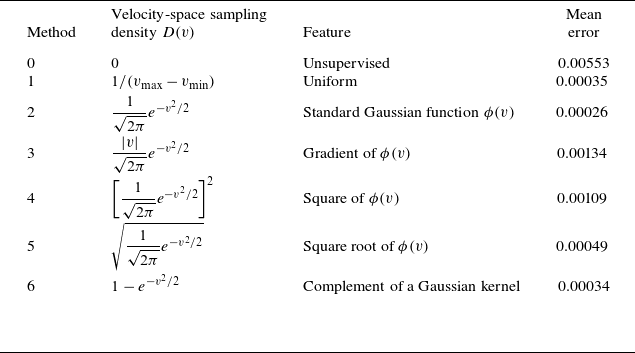
The mathematical expressions and characteristics of sampling functions
 $1$
–
 $6$
are summarised in table 1. Distributions of sampled data points are visualised in figure 5. Table 1 also records MAEs of the distribution function under different sampling methods. Figure 6 shows absolute values of electric potential
 $\phi$
at the centre of spatial space. Additionally, the evolution of the losses over training iterations is presented in figure 7.
Sampling methods of data points and collocation points.

Table 1. Long description
A table with seven rows and three columns. The columns are labeled Method, Velocity-space sampling density D(v), Feature, and Mean error. The rows list different sampling methods with their corresponding velocity-space sampling density functions, features, and mean errors. Row 1: Method 0, Velocity-space sampling density D(v) Unsupervised, Feature Unsupervised, Mean error 0.00553. Row 2: Method 1, Velocity-space sampling density D(v) 1/(v_max-v_min), Feature Uniform, Mean error 0.00035. Row 3: Method 2, Velocity-space sampling density D(v) (1/sqrt(2pi)) * e^(-v^2/2), Feature Standard Gaussian function φ(v), Mean error 0.00026. Row 4: Method 3, Velocity-space sampling density D(v) (|v|/sqrt(2pi)) * e^(-v^2/2), Feature Gradient of φ(v), Mean error 0.00134. Row 5: Method 4, Velocity-space sampling density D(v) [(1/sqrt(2pi)) * e^(-v^2/2)]^2, Feature Square of φ(v), Mean error 0.00109. Row 6: Method 5, Velocity-space sampling density D(v) sqrt[(1/sqrt(2pi)) * e^(-v^2/2)], Feature Square root of φ(v), Mean error 0.00049. Row 7: Method 6, Velocity-space sampling density D(v) 1 - e^(-v^2/2), Feature Complement of a Gaussian kernel, Mean error 0.00034.
Distribution of data points for different sampling methods
 $1$
–
 $6$
in table 1.

Compared with the unsupervised PINN, the data-driven PINN shows clear advantages in both convergence speed and simulation accuracy. In terms of convergence, after
 $50{\,}000$
training epochs, the loss of the unsupervised PINN remains of order
 $10^{-5}$
, whereas that of the data-driven PINN decreases to
 $10^{-8}$
. In terms of accuracy, the unsupervised PINN, used as a reference case, yields a relatively large MAE of
 $5.53\times 10^{-3}$
, while all data-driven cases achieve lower errors. These results indicate that incorporating data supervision can significantly improve the performance of PINNs.
Time evolution of electric potential magnitude in the middle of spatial space under different sampling methods.

History of training losses under different sampling methods.

Among the data-sampling strategies examined, the standard Gaussian sampling method gives the best overall performance, achieving the minimum MAE of
 $2.6\times 10^{-4}$
and the fastest convergence. In contrast, sampling method 3 gives the largest MAE among the data-driven cases,
 $1.34\times 10^{-3}$
, and its training process becomes unstable after approximately
 $3000$
epochs, with noticeable fluctuations in the loss function. The superior performance of Gaussian sampling can be attributed to its higher sampling density in the velocity-space region where wave–particle resonance is significant during Landau damping, allowing the model to better capture the dominant kinetic structures.
The standard deviation
 $\sigma$
of the Gaussian sampling distribution also affects accuracy. Figure 8 reports the relationship between the MAE
 $|\epsilon _a|$
and the standard deviation
 $\sigma$
. The number of supervised training data points is
 $100$
. The sampling-point density with
 $\sigma =2.5$
yields the best performance, resulting in MAE of
 $1.86\times 10^{-4}$
for the distribution function.
Relationship between standard deviation
 $\sigma$
of the Gaussian function and MAE
 $|\epsilon _a|$
.

Simulation result of the Vlasov–Poisson system based on data-supervised PINN under the supervision of 40, 400 and 4000 data points. Top: simulation errors for Landau damping with
 $k=0.5$
and
 $\epsilon =0.1$
. Bottom: simulation errors for Landau damping with
 $k=1$
and
 $\epsilon =0.4$
.

Figure 9. Long description
Panel A: A heat map showing simulation errors for Landau damping with parameters and. The x-axis ranges from 0 to 12, and the y-axis ranges from -6 to 6. The color scale ranges from -3.9 to 3.5 times 10^-3, with lighter colors indicating higher values. Panel B: A heat map showing simulation errors for Landau damping with 40 data points. The x-axis ranges from 0 to 12, and the y-axis ranges from -6 to 6. The color scale ranges from -3.9 to 3.5 times 10^-3, with lighter colors indicating higher values. Panel C: A heat map showing simulation errors for Landau damping with 400 data points. The x-axis ranges from 0 to 12, and the y-axis ranges from -6 to 6. The color scale ranges from -3.9 to 3.5 times 10^-3, with lighter colors indicating higher values. Panel D: A heat map showing simulation errors for Landau damping with 4000 data points. The x-axis ranges from 0 to 12, and the y-axis ranges from -6 to 6. The color scale ranges from -3.9 to 3.5 times 10^-3, with lighter colors indicating higher values. Panel E: A heat map showing simulation errors for Landau damping with parameters and. The x-axis ranges from 0 to 12, and the y-axis ranges from -6 to 6. The color scale ranges from -12.4 to 11.8 times 10^-3, with lighter colors indicating higher values. Panel F: A heat map showing simulation errors for Landau damping with 40 data points. The x-axis ranges from 0 to 12, and the y-axis ranges from -6 to 6. The color scale ranges from -12.4 to 11.8 times 10^-3, with lighter colors indicating higher values. Panel G: A heat map showing simulation errors for Landau damping with 400 data points. The x-axis ranges from 0 to 12, and the y-axis ranges from -6 to 6. The color scale ranges from -12.4 to 11.8 times 10^-3, with lighter colors indicating higher values. Panel H: A heat map showing simulation errors for Landau damping with 4000 data points. The x-axis ranges from 0 to 12, and the y-axis ranges from -6 to 6. The color scale ranges from -12.4 to 11.8 times 10^-3, with lighter colors indicating higher values.
4.2. Data-driven PINN solving the Vlasov–Poisson system
For the 1D1V Vlasov–Poisson system, the electric field is computed by FFT and the loss function of the Vlasov equation becomes
 \begin{align} & \mathcal{L}_{{\textit{PDE}}} = \left \lVert \partial _t \hat f(\boldsymbol{\cdot };\theta ) + v\frac {\partial \hat f(\boldsymbol{\cdot };\theta )}{\partial x} - \mathcal{F}^{-1}\!\left \{\frac {1-\int \hat f(x,v,t)\,{\rm d}v}{ik}\right \}\frac {\partial \hat f(\boldsymbol{\cdot };\theta )}{\partial v} \right \rVert ^2_{\varOmega \times (0,T]}.\nonumber \\& \end{align}
To ensure FFT compatibility, uniformly distributed collocation points on a Cartesian space–time grid are employed.
Data-driven training can accelerate the convergence of the Vlasov–Poisson system’s PINN model. Landau damping under different physical parameters is simulated. Figure 9 shows the errors under supervision of different numbers of data points, where
 $N_{data}$
represents the number of data points. The training data are randomly sampled, and the number of collocation points is
 $45\times 45\times 45=91\,125$
. Solving the Poisson equation by FFT proves effective in the data-driven solution of the Vlasov–Poisson system. The PINNs with more training data achieve higher convergence speed, while they can still provide reasonable approximations even with very sparse supervision using only 40 data points.
5. Unsupervised PINN solvers for the Vlasov–Poisson system
Due to the curse of dimension, it is difficult for classical numerical simulation to provide accurate simulation results of high-dimensional kinetic models. Therefore, in order to extend to high-dimensional problems, we directly solve the Vlasov–Poisson system based on unsupervised PINNs whose loss function only depends on physical equations and its initial and boundary conditions. As a preliminary study, 1D1V and 1D2V Vlasov–Poisson systems are firstly solved in this section.
5.1. Physics-informed neural network solvers for the 1D1V Vlasov–Poisson system
Figure 10 presents the distribution function and electric field results of a Landau damping process. In this case, the perturbation coefficient
 $\varepsilon$
is 0.4 and the wavenumber
 $k$
is 1, and the spatial domain of simulation covers two perturbation periods.
(a) Time evolution of the distribution function in a Landau damping simulation based on PINN, where the physical domain includes two periods. (b) The PINN result and exact solution of the distribution function
 $f(x = 2\pi ,v)$
at
 $t = 10$
. (c) The PINN solution of the electric field
 $E(x,t)$
.

The computational resource consumption of a PINN is mainly determined by the number of collocation points, which is particularly critical in high-dimensional numerical simulations. In the following text, we compare the accuracy of PINN and traditional finite-difference solvers (Perez Reference Perez2021) with different numbers of collocation points or grid points.
To make the comparison, we use an unsupervised PINN solver with different numbers of collocation points and a traditional FDM solver with different numbers of grid points. To better visualise the phase-mixing structures, the computational domain is chosen to contain two perturbation wavelengths,
 $x \in [0,4\pi /k]$
. Both the PINN collocation points and the FDM grid points are distributed on the same uniform grid, with
 $2N_x = N_v = N_t$
, where
 $N_x$
denotes the number of spatial grid points per wavelength,
 $N_v$
denotes the number of grid points in the
 $v$
direction and
 $N_t$
denotes the number of temporal grid points. Taking linear Landau damping as an example, we perform numerical simulations using the unsupervised PINN solver with the number of PDE collocation points ranging from
 $16^3$
to
 $90^3$
. To evaluate the accuracy of these solutions, a reference solution,
 $f_{\textrm{ref}}$
, is computed using the traditional FDM solver with a
 $128\times 128$
phase-space grid and 512 time steps. In the present Landau damping resolution test, the initial perturbation is prescribed as a single Fourier mode, and the comparison is restricted to the early linear stage of single-mode Landau damping.
Nevertheless, even in the linear Landau damping regime, phase mixing can generate increasingly fine structures in phase space. For the FDM solver, coarse grids may fail to resolve these fine structures. For the PINN solver, the solution is mesh-free and globally continuous, but sparse collocation points may not sufficiently constrain the PDE residual in regions with fine-scale structures. When
 $N_x$
reaches 12, the main phase-space structures can already be accurately captured, as shown in figure 11. The PINN performs well under a limited number of collocation points, whereas traditional FDM solvers require more grid points to achieve comparable accuracy, as illustrated in figure 12. When extended to high-dimensional problems, PINNs can reduce the cost associated with increasing the number of collocation points, thereby alleviating the curse of dimensionality.
Simulation results and absolute error of PINN and traditional FDM code under different numbers of grid points
 $N_x=8$
,
 $12$
and
 $45$
.

Absolute error
 $|\epsilon |$
versus grid resolution
 $N_x$
for the PINN and the traditional Vlasov solver based on the FDM. Here
 $N_x$
denotes the resolution of collocation points for the PINN and grid points for the traditional FDM Vlasov solver.

For high-dimensional problems, we usually focus on the balance between computational accuracy, efficiency and resources rather than pursuing extremely low numerical errors. Although traditional Vlasov solvers can achieve high accuracy using a fine grid, the computational cost is high. The PINN can achieve accurate numerical solutions using relatively sparse collocation points, which means we may require less GPU resources to solve simple high-dimensional problems. We discuss this issue in subsequent sections.
5.2. Physics-informed neural network solvers for 1D2V Vlasov–Poisson simulation
The direct Vlasov simulation of kinetic models has long been a major challenge in plasma physics, primarily due to their inherently high dimension. In a fully kinetic description of three-dimensional plasmas, the phase-space distribution function of charged particles,
 $f(x,y,z,v_x,v_y,v_z,t)$
, spans six dimensions. Even after gyro-averaging, the problem remains five-dimensional. As demonstrated in § 5.1, PINN solvers are capable of achieving relatively accurate solutions without dense collocation sampling, which gives them a distinct advantage in high-dimensional kinetic simulations. Motivated by the result above, we make a preliminary step towards higher-dimensional problems by simulating Landau damping in 1D2V phase space.
The initial condition is expressed by
 \begin{align} f(x,v_x,v_y,0) = \frac {1}{2\pi } {e}^{-(v_x^2+v_y^2)/2}(1+\epsilon \cos (kx)). \end{align}
The number of collocation points in the computational domain is set to
 $N_t\times N_x\times N_{v_x}\times N_{v_y} = 28\times 28\times 28\times 28$
. Figure 13 shows the simulation results of the electron distribution slices in two-dimensional velocity space at different times.
During the linear stage, the waves propagate along the
 $x$
direction, causing the distribution function to deform primarily along
 $v_x$
at the resonant points. Consequently, the two-dimensional velocity-space distribution function exhibits stripe-like structures on the velocity space
 $v_x{-}v_y$
, as shown in figure 13. The phase mixing on
 $x{-}v_x$
space is similar to that of 1D1V Landau damping.
Distribution function in 1D2V Landau damping simulated by PINN. Left: time evolution of the electron distribution on the
 $x{-}v_x$
phase space. Right: time evolution of the electron distribution on the two-dimensional velocity space
 $v_x{-}v_y$
.

Figure 13. Long description
Panel A: A series of heat maps showing the time evolution of the electron distribution on the phase space. The x-axis represents position (x) ranging from 0 to 6, and the y-axis represents velocity (vx) ranging from -4 to 4. The color scale on the right indicates the intensity of the distribution, with blue representing lower values and red representing higher values. Over time, the distribution evolves from a concentrated shape to a more spread-out pattern. Panel B: A series of heat maps showing the time evolution of the electron distribution on the two-dimensional velocity space. The x-axis represents velocity in the x-direction (vx) ranging from -4 to 4, and the y-axis represents velocity in the y-direction (vy) ranging from -4 to 4. The color scale on the right indicates the intensity of the distribution, with blue representing lower values and red representing higher values. Over time, the distribution evolves from a single peak to a more complex pattern with multiple peaks.
Compared with the 1D1V case, the training speed decreased from 20.41 to 3.95 iterations per second when 28 collocation points are used in each dimension. The GPU memory consumption is increased from 1742 MB to 23 402 MB, which is close to the memory limit of an NVIDIA RTX 4090 GPU (24 GB). In order to solve the 2D2V or higher-dimensional Vlasov–Poisson system on one RTX 4090 GPU, we have to reduce the number of collocation points on each dimension, which leads to increased errors or even numerical failure (Krishnapriyan et al. Reference Krishnapriyan, Gholami, Zhe, Kirby and Mahoney2021). Inadequate collocation points degrade accuracy and may prevent convergence; in particular, they may cause the predicted distribution to collapse to the Maxwellian equilibrium.
As a novel numerical solver, standard PINNs currently demonstrate advantages with relatively sparse collocation points, showing their potential in high-dimensional kinetic simulations. In the following section, to further improve the feasibility of PINN-based solvers for high-dimensional Vlasov–Poisson systems, we introduce a PINN variant designed to reduce memory consumption and training time.
6. Separable PINN solvers for Vlasov–Poisson simulation
6.1. Introduction to SPINN
In recent years, advanced architectures of PINNs have been developed to accelerate training and reduce memory usage. A SPINN is an MLP architecture designed to reduce computational cost by exploiting separability of input dimensions and forward-mode AD (Cho et al. Reference Cho, Nam, Yang, Yun, Hong and Park2023). Instead of mapping full dimensional coordinates through a single multi-input MLP, the SPINN uses several one-dimensional subnetworks.
The SPINN is applied to the Vlasov–Poisson system. The solution is expressed as a low-rank CP tensor expansion (Cho et al. Reference Cho, Nam, Yang, Yun, Hong and Park2023) as shown in figure 14:
 \begin{align} \hat f = \sum _{j=1}^{r}\left (\prod _{p=1}^{P} f_{\theta _{x_p},j}(x_p)\prod _{q=1}^{Q} f_{\theta _{v_q},j}(v_q) f_{\theta _t,j}(t)\right ), \end{align}
where
 $\hat {f}$
is the predicted PDE solution,
 $x_1,\ldots ,x_P,v_1,\ldots ,v_Q,t$
are the inputs,
 $P$
and
 $Q$
are the dimensions of spatial and velocity space and
 $f_{\theta _i,j}(x_p)$
and
 $f_{\theta _i,j}(v_q)$
are the
 $j$
th components of the output from corresponding body networks. Each subnetwork
 $(f_{\theta _i}:\mathbb{R}\to \mathbb{R}^r)$
maps the
 $i$
th input coordinate to an
 $r$
-dimensional feature representation, where
 $r$
denotes the separation rank.
Construction of a SPINN framework for solving the Vlasov–Poisson system. Here,
 $1\leqslant p\leqslant P$
and
 $1\leqslant q\leqslant Q$
, where
 $P$
is the dimension of physical space and
 $Q$
is the dimension of velocity space.

For a standard PINN, the number of network evaluations at collocation points scales as
 $O(\prod _{i=1}^{I} N_i)$
theoretically, where
 $N_i$
is the number of collocation points along the
 $i$
th dimension and
 $ I = P + Q + 1$
. In contrast, SPINN evaluates
 $I$
single-input subnetworks on their respective collocation points. The number of evaluations scales as
 $O(\sum _{i=1}^{I} N_i)$
, while the remaining products and summations are comparatively inexpensive. Therefore, the SPINN framework can reduce the cost of evaluating PDE residuals, thereby accelerating training and reduce GPU memory consumption (Cho et al. Reference Cho, Nam, Yang, Yun, Hong and Park2023).
In the SPINN for the Vlasov–Poisson system, the PDE loss is computed via forward-mode AD on the collocation points, whereas parameter updates are performed with standard back-propagation. All of the MLP subnetworks are activated by tanh function. The Poisson equation is solved by FFT as described earlier.
The SPINN is first used to simulate the Landau damping case of § 5.1. For the standard PINN used there, the upper limit of collocation points for the 1D1V problem is
 $N_t\times N_x \times N_v = 92\times 92\times 92$
when running on a single NVIDIA RTX 4090 GPU with
 $24$
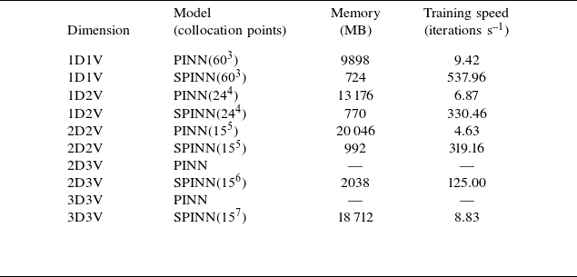
GB of memory. For the SPINN, memory consumption is substantially reduced, enabling us to extend simulations to longer spatial and temporal domains and further explore nonlinear cases. The GPU memory consumptions of standard PINN and SPINN for multi-dimensional problems are presented in table 2. Problems with dimensions higher than 2D2V are not suitable to be solved by standard PINN due to exceeding of memory requirements. Moreover, SPINN achieves significant training acceleration because of its lower cost of network evaluations.
Memory consumption and training speed of PINN and SPINN for multi-dimensional Vlasov–Poisson systems.

Table 2. Long description
The table presents data on memory consumption and training speed for different models of PINN and SPINN across various dimensions of Vlasov-Poisson systems. It includes five columns: Dimension, Model (with collocation points), Memory (MB), and Training speed (iterations per second). The table has eight rows, each representing a different dimensional problem. Row 1: Dimension 1D1V, Model PINN(60^3), Memory 9898 MB, Training speed 9.42 iterations per second. Row 2: Dimension 1D1V, Model SPINN(60^3), Memory 724 MB, Training speed 537.96 iterations per second. Row 3: Dimension 1D2V, Model PINN(24^4), Memory 13176 MB, Training speed 6.87 iterations per second. Row 4: Dimension 1D2V, Model SPINN(24^4), Memory 770 MB, Training speed 330.46 iterations per second. Row 5: Dimension 2D2V, Model PINN(15^5), Memory 20046 MB, Training speed 4.63 iterations per second. Row 6: Dimension 2D2V, Model SPINN(15^5), Memory 992 MB, Training speed 319.16 iterations per second. Row 7: Dimension 2D3V, Model PINN, Memory not specified, Training speed not specified. Row 8: Dimension 2D3V, Model SPINN(15^6), Memory 2038 MB, Training speed 125.00 iterations per second. Row 9: Dimension 3D3V, Model PINN, Memory not specified, Training speed not specified. Row 10: Dimension 3D3V, Model SPINN(15^7), Memory 18712 MB, Training speed 8.83 iterations per second.
6.2. The 1D1V and 1D2V Vlasov–Poisson simulations based on SPINN
Using SPINN, the Landau damping problem can be solved with much denser temporal collocation points, enabling the distribution function to be evolved over a longer time interval. Landau damping is simulated from
 $t=0$
to
 $t=30$
, with collocation points uniformly set to
 $N_t\times N_x \times N_v = 1000\times 250\times 250$
. The result shown in figure 15 depicts the time evolution of the electron distribution in phase space, with a maximum error of
 $1.724\times 10^{-2}$
.
Simulation results of Landau damping from
 $t=0$
to
 $t=30$
based on SPINN. Top: time evolution of the distribution function in 1D1V phase space. Bottom: SPINN result and reference solution of the distribution function
 $f(x=\pi ,v)$
at
 $t=10$
,
 $20$
and
 $30$
.

High resolution of collocation points also enables SPINN to approach nonlinear cases which are more complex, such as two-stream instabilities. Simulation is implemented with
 $N_t\times N_x\times N_v = 300\times 300\times 300$
collocation points. The initial parameters in (4.5) are
 $\epsilon =0.05$
,
 $k=0.2$
and
 $v_0=2.4$
. The formation process of a vortex structure in phase space is shown in figure 16. Since changes of distribution function are relatively minor at early times, the simulation can be carried out over a much longer time domain, from
 $t=0$
to
 $t=12$
.
Simulation result of two-stream instabilities based on SPINN: formation of phase-space holes.

In the later stage of two-stream instability, the distribution of electrons develops complex phase-space structures (Hou et al. Reference Hou, Yu, Wang, Liu, Chen and Wu2024; Einkemmer et al. Reference Einkemmer, Li, Mouhot and Yue2025). Long-time simulations are usually less accurate due to limited collocation points and increased training difficulty. To maintain the accuracy of simulation, the Vlasov–Poisson system is not solved in the full time interval. Instead, data of distribution functions at
 $t=12$
, 20, 25 are generated from the open-source code (Perez Reference Perez2021) and then used as the initial conditions for evolving the electron distribution in later stages. In figure 17, the Vlasov–Poisson system is solved in these time intervals:
 $t\in [12,20]$
,
 $t\in [20,25]$
and
 $t\in [25,30]$
, demonstrating the feasibility of the proposed method for simulating two-stream instabilities.
Multi-stage simulation results of two-stream instabilities based on SPINN: time evolution of the electron distribution from
 $t=12$
to
 $t=30$
.

Magnetised plasmas are ubiquitous in fusion devices and space environments, where the background magnetic fields influence transport, stability and wave–particle interactions. For magnetised plasmas, electron cyclotron effects should be captured. In the following text, we explore the effectiveness of SPINN for simulating magnetised plasma in 1D2V phase space, where the magnetic field
 $B_0$
is aligned with the z axis. The normalised 1D2V Vlasov equation for magnetised plasma can be expressed as
 \begin{align} \frac {\partial f(x,v_x,v_y,t)}{\partial t} &+ v_x\frac {\partial f(x,v_x,v_y,t)}{\partial x} - \bigl (E(x,t)+v_y B_0\bigr )\frac {\partial f(x,v_x,v_y,t)}{\partial v_x}\nonumber \\&+ v_x B_0\frac {\partial f(x,v_x,v_y,t)}{\partial v_y} = 0. \end{align}
In this implementation, the number of collocation points is
 $N_t\times N_x\times N_{v_x}\times N_{v_y}=160\times 80\times 80\times 80$
. The initial condition is still a disturbed Maxwellian distribution with
 $k=0.75$
,
 $\epsilon =0.2$
and the magnitude of the external magnetic field
 $B_0=0.5$
. Figure 18 presents the time evolution of electron distribution in two-dimensional velocity space, including the case of unmagnetised plasma and magnetised plasma. The electric field energy decays during the linear damping stage and then suddenly increases, showing a magnetised nonlinear trapping (Valentini et al. Reference Valentini, Veltri and Mangeney2005a
,Reference Valentini, Veltri and Mangeney
b
). The evolution of electric field energy under varying magnetic field intensities is shown in figure 19, which demonstrates that stronger magnetic fields induce earlier nonlinear effects.
Time evolution of distribution function and electric field in the 1D2V Vlasov–Poisson simulation. Top: linear Landau damping in unmagnetised plasma (
 $B_0=0.0$
). Bottom: nonlinear resonance in magnetised plasma (
 $B_0=0.5$
).

Figure 18. Long description
The image contains multiple heat maps and contour plots. The top row shows linear Landau damping in unmagnetised plasma, while the bottom row shows nonlinear resonance in magnetised plasma. Each row consists of six contour plots and one heat map. The contour plots are labeled with time values t ranging from 0 to 15. The axes for the contour plots are labeled vx and vy, representing velocity components. The heat maps have axes labeled x and t, representing position and time, respectively. The color scales indicate the magnitude of the distribution function and electric field. The top row shows the evolution of the distribution function over time in unmagnetised plasma, with the heat map displaying the electric field. The bottom row similarly shows the evolution in magnetised plasma, with the heat map indicating the electric field. The contour plots illustrate the changes in the distribution function at specific time intervals.
Time evolution of electric field energy for varying magnitude of external field
 $B_0$
. Linear damping is followed by magnetised nonlinear trapping.

6.3. High-dimensional Vlasov–Poisson simulation based on SPINN
A critical aim of this work is to investigate the feasibility of PINNs for high-dimensional Vlasov–Poisson simulation. Standard PINNs have been tested for 1D1V and 1D2V problems, but they suffer from computational burden, including GPU memory constraints and slow training, which makes them unsuitable for higher-dimensional problems. Since SPINN solvers are advantageous in terms of memory consumption and training efficiency compared with standard PINNs, they are applied to 2D2V, 2D3V and 3D3V Vlasov–Poisson simulations. For simplicity, only electrostatic Landau damping is considered in these preliminary tests by solving the linearised Vlasov–Poisson system.
Time evolution of the perturbation quantities. Top: time evolution of distribution function perturbation
 $\delta f$
visualised in velocity space. Bottom: time evolution of electric field components
 $E_x$
and
 $E_y$
.

For the 2D2V Landau damping case, the initial condition is given by
 \begin{align} \delta f_0 = \frac {1}{2\pi }{e}^{-(v_x^2+v_y^2)/2}\bigl (\epsilon _x\cos (k_x x)+\epsilon _y\cos (k_y y)\bigr ), \end{align}
where
 $k_x=k_y=0.5$
and
 $\epsilon _x=\epsilon _y=0.1$
. Figure 20 depicts the time evolution of the phase-space distribution: the perturbation develops block-like structures in the
 $v_x{-}v_y$
plane, and the electric field components decay. From the time evolution of the electric field energy (figure 21), we calculate the damping rate
 $\gamma = 0.1516$
and the frequency
 $\omega = 1.3931$
, which are close to the theoretical values of
 $\gamma _{{t}} = 0.1534$
and
 $\omega _{{t}} = 1.4157$
(Filbet & Sonnendrucker Reference Filbet and Sonnendrucker2003). The relative errors are
 $1.17\,\%$
and
 $1.60\,\%$
, respectively.
Time evolution of the electric field energy for the 2D2V linear Landau damping problem. The damping rate and real frequency are consistent with theoretical analysis.

For the 2D3V simulation of linear Landau damping, the number of collocation points is
 $N_t \times N_x \times N_y \times N_{v_x} \times N_{v_y} \times N_{v_z} = 36\times 16\times 16\times 12\times 12\times 12 = 15{\,}925{\,}248$
, which consumes
 $3{}618$
MB of GPU memory. The initial distribution is
 \begin{align} \delta f_0 = \frac {1}{(2\pi )^{3/2}} {e}^{-(v_x^2+v_y^2+v_z^2)/2}\bigl (\epsilon _x\cos k_x x + \epsilon _y\cos k_y y\bigr ), \end{align}
where
 $k_x=k_y=0.6$
and
 $\epsilon _x=\epsilon _y=0.1$
. Figure 22 presents the three-dimensional electron distribution in velocity space at the centre of the spatial domain, and figure 23 depicts the time evolution of the distribution on the
 $v_x{-}v_y$
plane at
 $v_z=0$
. Resonance induced by the two-dimensional initial perturbation can be observed on the
 $v_x{-}v_y$
plane. Time evolution of the electric field energy is depicted in figure 24, and the relative error of damping rate is 2.65 %.
Perturbation of the electron distribution function
 $\delta f$
in three-dimensional velocity space at the centre of two-dimensional spatial space when
 $t=4.5$
.

Time evolution of distribution function perturbation
 $\delta f$
on the
 $v_x{-}v_y$
plane at the centre of two-dimensional spatial space, where
 $v_z=0$
.

Time evolution of the electric field energy for the 2D3V linear Landau damping problem.

Finally, the SPINN solver is extended to 3D3V phase space. The number of collocation points is
 $N_t \times N_x \times N_y \times N_z \times N_{v_x} \times N_{v_y} \times N_{v_z} = 36 \times 13 \times 13 \times 13 \times 12 \times 12 \times 12 = 136{\,}670{\,}976$
, which consumes
 $6712$
MB of GPU memory. To simulate Landau damping, the initial distribution is set as
 \begin{align} \delta f_0 = \frac {1}{(2\pi )^{3/2}} {e}^{-(v_x^2+v_y^2+v_z^2)/2}\bigl (\epsilon _x\cos k_x x + \epsilon _y\cos k_y y + \epsilon _z\cos k_z z\bigr ). \end{align}
A simple result of linear Landau damping is shown in figure 25, where
 $k_x=k_y=k_z=0.9$
and
 $\epsilon _x=\epsilon _y=\epsilon _z=0.1$
. This figure visualises the electron distribution in three-dimensional velocity space at the centre of physical space. Resonant structures associated with the three imposed wave propagation directions can be observed in velocity space. Electron distribution on the
 $v_x{-}v_y$
plane is visualised in figure 26. Time evolution of the electric field energy is shown in figure 27, and the relative error of damping rate is 4.11 %.
Perturbation of the electron distribution function
 $\delta f$
in three-dimensional velocity space, at the centre of three-dimensional physical space, when
 $t=2.0$
.

Figure 25. Long description
A 3D scatter plot representing the perturbation of the electron distribution function in three-dimensional velocity space. The plot is centered in three-dimensional physical space. The horizontal axis is labeled vx, the vertical axis is labeled vy, and the depth axis is labeled vz. Each dot represents a data point in the velocity space. The color of the dots ranges from blue to red, indicating different values, with a color bar on the right showing the scale from -8 times 10 to the power of -5 to 8 times 10 to the power of -5. The plot shows a spherical distribution with varying values across the surface.
Time evolution of distribution function perturbation
 $\delta f$
on the
 $v_x{-}v_y$
plane, at the centre of three-dimensional physical space, where
 $v_z=0$
.

Time evolution of the electric field energy for the 3D3V linear Landau damping problem.

Throughout this section, all SPINN models are trained on a single NVIDIA RTX 4090 GPU with 24 GB of memory. These high-dimensional tests illustrate the motivation for using SPINN in kinetic simulations. For a conventional grid-based Vlasov solver, the number of degrees of freedom scales as the product of the grid points in all phase-space dimensions, leading to rapidly increasing memory and storage requirements. In contrast, a PINN represents the unknown solution with a neural network and trains the network by minimising the residuals of the governing PDEs. Since it does not rely on a grid-based discretisation of the high-dimensional kinetic equations, it is regarded as a mesh-free method. Moreover, the separable representation used in SPINN reduces the cost of evaluating the residuals of high-dimensional PDEs and provides a more efficient representation of the high-dimensional distribution function, thereby significantly reducing the training time and GPU memory consumption compared with standard PINNs.
For 1D1V problems, when using the collocation-point grid listed in table 2, the SPINN model requires approximately 10 minutes to complete training, whereas the FDM reference code on the same grid finishes computation within one minute. Taking the 2D2V case in figure 21 as an example, SPINN generally requires about 5 hours to converge to an accurate solution, evolving from
 $t = 0$
to
 $t = 6\omega _p^{-1}$
. In comparison, the computational cost of traditional solvers for 2D2V simulations varies significantly depending on the numerical algorithm, parameter settings, computing platform and the specific physical problem considered, with reported computational times ranging from tens of minutes to tens of hours (Kormann Reference Kormann2015; Ho & Vogman Reference Ho and Vogman2025). For example, a full-grid Landau damping simulation reported in Kormann (Reference Kormann2015) used a
 $32^2 \times 128^2$
phase-space grid, evolved the system up to
 $30\omega _p^{-1}$
and required approximately 17.2 h of computational time. For 3D3V problems, the SPINN solver requires about 10 h to complete a simulation up to
 $5\omega _p^{-1}$
on one RTX 4090 GPU, while such 3D3V simulations require very large memory and computational resources and are usually performed with specialised massively parallel implementations. The reported computational costs vary greatly among different test cases, algorithms, resolutions and computing platforms, making a direct comparison difficult (Einkemmer & Moriggl Reference Einkemmer and Moriggl2023; Kirchhart & Wilhelm Reference Kirchhart and Wilhelm2024).
Furthermore, high-dimensional numerical simulations typically generate voluminous output grid data that demand substantial disk storage. In contrast, for PINN and SPINN solvers, we only need to retain the network parameters after training, thus only several hundred kilobytes of disk storage are required. The solution can be predicted at arbitrary points in phase space without storing the full multi-dimensional grid data. In other words, PINN and SPINN provide globally continuous and differentiable numerical solutions, enabling rapid storage and reconstruction.
7. Summary and discussion
This work focuses on solving the Vlasov–Poisson system using PINN and SPINN. The loss functions include residuals of the Vlasov equation together with initial and boundary conditions, and the self-consistent electric field is solved through the Poisson equation by FFT. We implemented data-supervised PINN frameworks for solving both the Vlasov equation and the Vlasov–Poisson system in 1D1V phase space, and conducted evaluations and optimisations of collocation-point and data-point sampling. Data supervision accelerates convergence and improves simulation accuracy. In future work, experimental measurements could be used together with physical equations to impose joint data–physics constraints during PINN training.
Moreover, unsupervised PINN solvers are constructed to directly solve the Vlasov–Poisson system, and they remain effective under relatively sparse collocation points. The 1D2V simulations are also implemented within this framework. Standard PINNs are shown to be feasible for solving the Vlasov–Poisson system, but their relatively high memory consumption and low training efficiency restrict their ability to simulate problems of higher dimension or higher accuracy.
We therefore apply SPINN, a variant of PINN, for better simulation performance. This separable framework utilises multiple one-dimensional subnetworks and combines their output features via element-wise products, reducing memory consumption and substantially accelerating training. The SPINN can better simulate Landau damping over longer time intervals and is also suitable for nonlinear cases such as two-stream instability and nonlinear resonance in magnetised plasma. Furthermore, Landau damping in 2D2V, 2D3V and 3D3V phase space is simulated on a single RTX 4090 GPU.
In summary, PINNs for kinetic equations do not rely on fixed grids or a large number of collocation points. Once trained, the neural network provides a globally continuous and differentiable representation of the solution, enabling reconstruction at arbitrary points in phase space and time with a relatively low storage cost. In addition, PINNs can naturally incorporate both physical constraints and experimental or numerical data. The SPINN variant further reduces the computational cost of high-dimensional problems through its separable architecture, providing a possible route for performing preliminary high-dimensional kinetic simulations on a single GPU or even on personal computers.
In future work, we plan to extend the physical model to the Vlasov–Maxwell system with more particle species, and to implement kinetic simulations in tokamak geometry, especially for nonlinear problems. At the same time, we will investigate improved neural-network frameworks and training algorithms in order to capture weak perturbations and nonlinear processes over longer time intervals. Finally, the potential of SPINN in high-dimensional problems and plasma wave simulations will be further explored.
Acknowledgements
Editor Luís O. Silva thanks the referees for their advice in evaluating this article.
Funding
The authors from Dalian University of Technology were supported by the National Natural Science Foundation of China (grant nos. 12435014 and 12575227) and the National MCF Energy R&D Program of China (grant no. 2024YFE03160002).
Declaration of interests
The authors report no conflict of interest.


 f
 t=10
 f
 x=π/k
 E(x,t)
 E(x,t)

 f(x,v)
 f(x,v)
 t=50

 1
 6


 σ
 |ϵa|

 k=0.5
 ϵ=0.1
 k=1
 ϵ=0.4

 f(x=2π,v)
 t=10
 E(x,t)

 Nx=8
 12
 45

 |ϵ|
 Nx
 Nx

 x−vx
 vx−vy

 1⩽p⩽P
 1⩽q⩽Q
 P
 Q

 t=0
 t=30
 f(x=π,v)
 t=10
 20
 30


 t=12
 t=30

 B0=0.0
 B0=0.5

 B0

 δf
 Ex
 Ey


 δf
 t=4.5

 δf
 vx−vy
 vz=0


 δf
 t=2.0

 δf
 vx−vy
 vz=0


 Open access

