1. Introduction
The increasing availability and popularity of survey data enable us to verify if professionals believe in simple models often used as crucial building blocks for larger economic models. One prominent example is the so-called Taylor (Reference Taylor1993) rule and the ideal case to study the expectation formation mechanism in the context of the Taylor rule is provided by the European Central Bank (ECB) and the professionals monitoring and forecasting its policy. In this vein, the ECB Survey of Professional Forecasters (SPF) directly asks participants to reveal their view about the future development of the policy rate in contrast to other surveys providing forecasts for market interest rates. Therefore, in this article, we study whether professional forecasters form their expectations regarding the policy rate of the ECB consistent with the Taylor rule and whether the expectation building mechanism has changed over the recent two decades.
Following the original version of the Taylor (Reference Taylor1993) rule, the nominal policy rate
 $i_t$
should be set in reaction to deviations of the inflation rate
 $\pi_t$
from its target
 $\pi_t^*$
and of GDP
 $y_t$
from its potential
 $\overline{y}_t$
 \begin{equation}i_t=\pi_t+r_t^*+\phi_1\left(\pi_t-\pi_t^*\right)+\phi_2\left(y_t-\overline{y}_t\right).\end{equation}
 $r_t^*$
denotes the equilibrium real interest rate consistent with an output gap
 $y_t-\overline{y}_t$
equal to zero and
 $\phi_1>0$
as well as
 $\phi_2>0$
. Taylor (Reference Taylor1993) proposes
 $\phi_1=\phi_2=0.5$
and the rationale is to tighten monetary policy by increasing the policy rate when inflation is above its target and/or output is above its potential. In the opposite situation, the rule recommends a decrease of the policy rate to stimulate economic activity. Subsequent studies have shown that estimations of policy reaction functions in the sense of equation (1) based on ex post revised data are not reliable (Orphanides, Reference Orphanides2001) and emphasize the importance of forward-looking versions of equation (1) by replacing the actual inflation rate by an expected value (Clarida et al., Reference Clarida, Galí and Gertler1998, Reference Clarida, Galí and Gertler1999, Reference Clarida, Galí and Gertler2000; Orphanides, Reference Orphanides2003). Malmendier et al. (Reference Malmendier, Nagel and Yan2021) also follow this notion but additionally introduce heterogeneity in inflation expectations across individuals. In this study, we proceed in the same direction and replace all components by expectations of professionals and also allow for heterogeneity across professional forecasters. In addition, we further exploit the cross-sectional variation inherent in our survey data set and also test whether the Taylor rule relationship provided in equation (1) translates into a connection between forecasters’ disagreement regarding the policy rate, inflation, and GDP growth.
This article also relates to studies by Fendel et al. (Reference Fendel, Frenkel and Rülke2011) and Pierdzioch et al. (Reference Pierdzioch, Rülke and Stadtmann2012), who use survey data to estimate monetary policy reaction functions for G7 economies and for the United States (US) based on data from Consensus Economics and the Livingston survey, respectively.Footnote 1 Gorter et al. (Reference Gorter, Jacobs and De Haan2008) also rely on data from Consensus Economics to estimate a Taylor rule for the ECB but they do not study expectation formation as they use realized interest rates on the left-hand side of their Taylor rule and solely rely on mean forecasts across individual forecasters for inflation and GDP growth. They do not exploit the heterogeneity in individual forecasts. In addition, their sample period ends in December 2006 and therefore also does not cover the turbulent times of ECB policy since the global financial crisis. The only other study also using the ECB SPF data set for the estimation of the Taylor rule is provided by Frenkel et al. (Reference Frenkel, Lis and Rülke2011). We extend their study into several directions: first, we exploit the cross-sectional variation by estimating a dynamic fixed-effects model while also accounting for a potential Nickell (Reference Nickell1981) bias and by relying on individual reaction functions. Second, we also study changes over time by adding nearly 10 years of most recent data, which includes the crisis period and the zero lower bound period. Third, we also assess whether the Taylor rule might provide the foundation for the co-movement in disagreement among forecasters regarding the three variables of interest. Therefore, we extend the existing literature by the estimation of Taylor rule-type reaction functions based on individual expectations included in survey data for the Euro Area and provide important insights into the expectations formation mechanism of professionals. A clear benefit of the ECB SPF data set is the fact that it includes forecasts for the ECB policy rate in contrast to other sources such as Consensus Economics, which solely include forecasts for money market rates (e.g. 3-month interest rates) that can only serve as a proxy for the policy rate. This offers the possibility to examine directly whether professionals believe in the concept of the Taylor rule when forming their expectations.
The remainder of the article is organized as follows. Section 2 describes our data set. Section 3 presents our empirical framework and our main findings while Section 4 concludes.
2. Data
Our empirical study is based on micro-level data from the ECB SPF spanning a quarterly sample period from 2002Q1 to 2020Q2. The ECB initiated this SPF together with the introduction of the euro in 1999 and started asking all participants to provide fixed-event as well as fixed-horizon forecasts regarding inflation, real GDP growth, and unemployment for the Euro Area (EA) at the beginning of each quarter. In 2002Q1, the SPF has been extended to also cover forecasts regarding the policy rate of the ECB, that is, the rate of main refinancing operations (MRO), as part of the assumptions upon which forecasters base their inflation and GDP growth forecasts. Therefore, the start of our sample period is restricted by the availability of MRO rate forecasts in the ECB SPF. In this study, we rely on forecasts for the MRO rate, inflation, and real GDP growth as proxies for expectations of professionals to examine if they form their expectations in line with the concept of the Taylor rule.
More precisely, we use so-called rolling horizon forecasts for the month (quarter) 1-year ahead of the latest available observation at the time the survey is conducted for inflation (real GDP growth). This means that, for example, for inflation forecasts made in Q1, the latest available observation is from December of the previous year and therefore the forecast is made for December 1-year ahead. In case of real GDP growth forecasts made in Q1, the latest available observation is from Q3 of the previous year. Therefore, in this case, the forecast is made for Q3 1-year ahead. This means that although the period being forecasted is not identical for inflation and GDP growth, we use in both cases 1-year ahead forecasts made at the same time using the latest available information. Fixed-horizon forecasts for consecutive quarters are not provided within the survey for inflation and GDP growth. These 1-year ahead forecasts correspond to the forecast horizon of
 $h=4$
quarters. To match this horizon, we have also selected the four quarters ahead forecasts for the MRO rate. In contrast to inflation and GDP growth forecasts, participants are asked to provide forecasts for four consecutive quarters starting with the quarter when the survey is conducted for the MRO rate.
This data set has often been considered in previous studies concerning the evaluation of forecasts and the expectation building mechanism regarding inflation, GDP growth, unemployment, or the crude oil price (see e.g. Reitz et al., Reference Reitz, Rülke and Stadtmann2012; Andrade and Le Bihan, Reference Andrade and Le Bihan2013; Dovern, Reference Dovern2015; Abel et al., Reference Abel, Rich, Song and Tracy2016). We add to this strand of the literature by using this data set to assess whether professional expectations are formed consistent with the Taylor rule. Professional forecasters participating in the ECB SPF include forecast units of several different institutions within the EA such as banks or research institutes. These professionals can be considered as most informed economic agents, which are mostly familiar with the general concept of the Taylor rule and/or the reasoning behind it. The number of participating forecasters varies over time, ranges between 41 and 61 within the sample period and totals 103 different institutions.
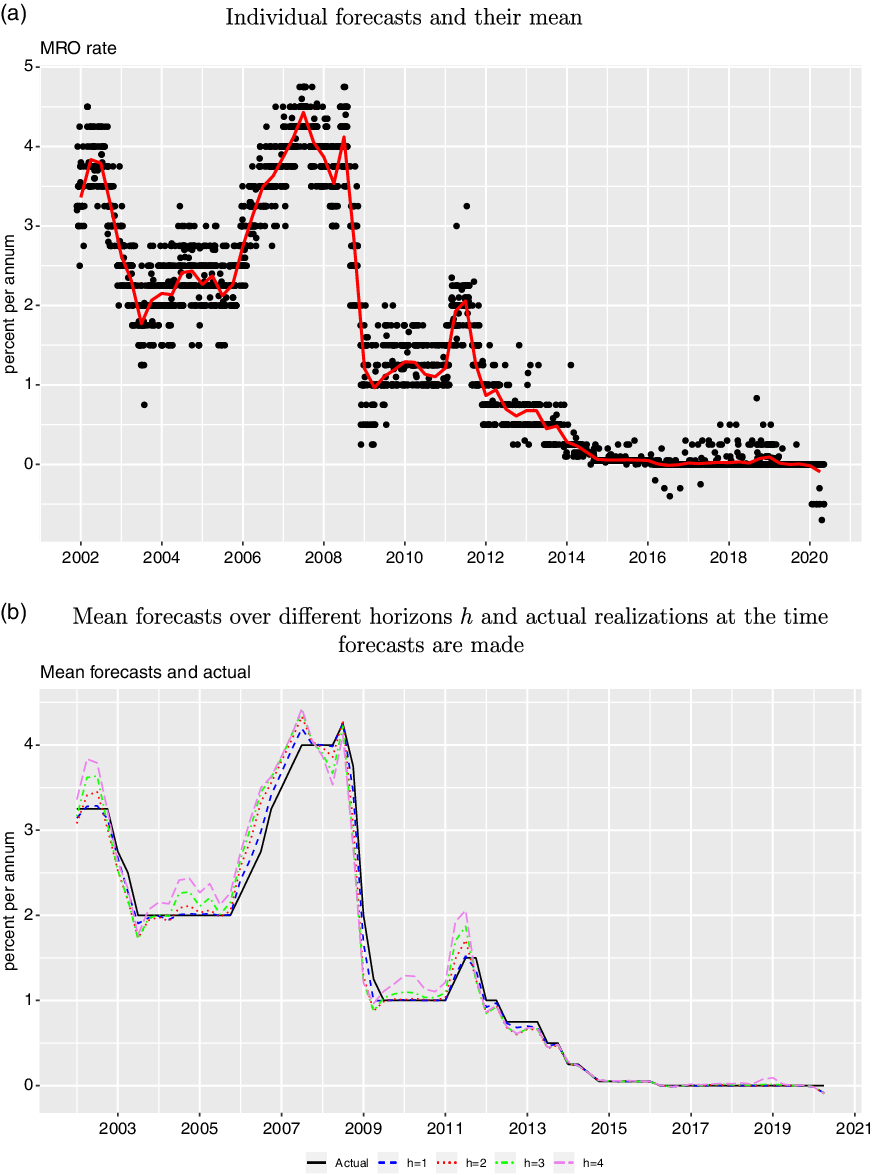
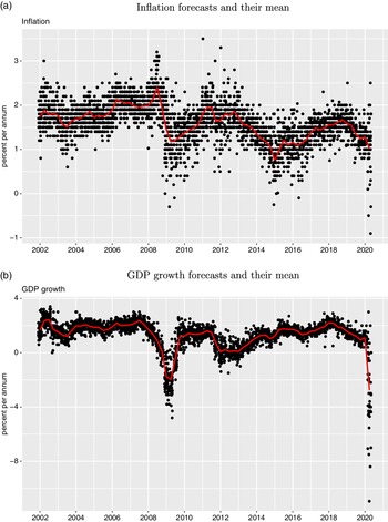
Panel (a) in Figure 1 displays individual quarterly four quarters ahead MRO rate point forecasts (black points) together with the corresponding mean forecasts across individual forecasters (red line) for the period from 2002Q1 to 2020Q2. The points around the red line illustrate the disagreement across forecasters regarding the future monetary policy rate of the ECB. It becomes evident that the disagreement among forecasters clearly decreased in the latest period characterized by a policy rate of (nearly) zero but it has not disappeared completely. This indicates that several forecasters have also expected changes in the stance of monetary policy within this period. Panel (b) compares mean forecasts for the policy rate across forecasters over four different forecast horizons with the actual realization of the MRO rate at the time forecasts are made, which exactly matches the dates at which forecasters had to submit their forecasts. This graph illustrates that mean forecasts are closely attached to the current policy rate but also shows forecasters’ expectations about a potential change in the policy rate. Figure 2 also visualizes individual and mean forecasts for inflation and GDP growth and explicitly shows a stronger disagreement among forecasters and a substantial downturn of real GDP growth in the latest period (i.e. 2020Q2) due to the impact of the COVID-19 pandemic.
Individual and mean forecasts for the ECB policy rate.
The plots show quarterly time series of the ECB rate for main refinancing operations (MRO) forecasts (in percent per annum) across individual forecasters (black points) together with mean forecasts across individuals (red line) for the period from 2002Q1 to 2020Q2 and for the forecast horizon of four-quarters-ahead. The data has been taken from the ECB Survey of Professional Forecasters (SPF).

Individual and mean forecasts for inflation and GDP growth.
The plots show quarterly time series of Euro Area inflation and real GDP growth forecasts (in percent per annum) across individual forecasters (black points) together with mean forecasts across individuals (red line) for the period from 2002Q1 to 2020Q2 and for the forecast horizon of four-quarters-ahead. The data has been taken from the ECB Survey of Professional Forecasters (SPF).

The data set includes variation across forecasters (
 $j=1,\ldots,n$
) and over time (
 $t=1,\ldots,T$
).
 $T=74$
while n varies between 41 and 61. As both dimensions (i.e. cross-section and time) are of medium size, our estimations benefit from the panel dimension in terms of efficiency by exploiting variation across forecasters and over time. However, in further robustness checks, we also switch to the time series perspective relying on the mean across forecasters and also on individual estimates.
3. Empirical framework and findings
Our empirical implementation of equation (1) consists of a fixed-effects model exploiting the heterogeneity across forecasters and the variation over time
 \begin{align}E_{j,t}\left(i_{t+h}\right) & = \phi_{1}\left[E_{j,t}(\pi_{t+h})-\pi^*\right]+\phi_{2}\left[E_{j,t}\left(\Delta y_{t+h}\right)-\overline{E}_{t}^*\left(\Delta y_{t+h}\right)\right]+\phi_{3}E_{j,t-1}\left(i_{t+h}\right)\nonumber\\[3pt]& +\mu_j+\lambda_t+\varepsilon_{j,t+h},\end{align}
where
 $E_{j,t}(.)$
denotes the forecast for the period
 $t+h$
made in t by forecaster j,
 $i_{t}$
stands for the ECB policy rate,
 $\pi_t$
represents EA inflation and
 $\Delta y_{t}$
denotes EA real GDP growth.
 $\pi^*$
stands for the inflation target rate of the ECB and equals 2% and
 $\overline{E}_{t}^*(\Delta y_{t+h})$
represents EA potential GDP growth measured by Hodrick–Prescott-filtered GDP growth mean forecasts across forecasters with a smoothing parameter
 $\lambda=1600$
.Footnote 2 In addition, it is common practice in the Taylor rule literature to account for interest rate smoothing by including the one-period-lagged policy rate due to the tendency of central banks to change its policy rate gradually. In contrast, we include the previous periods’ expectations about the future policy rate
 $E_{j,t-1}(i_{t+h})$
due to the fact that this article focuses on the expectations building process and previous studies have also provided evidence for the sluggishness of economic forecasts due to the presence of information rigidities (Coibion and Gorodnichenko, Reference Coibion and Gorodnichenko2015).Footnote 3 Individual fixed and time fixed effects
 $\mu_j$
and
 $\lambda_t$
allow for a potential heterogeneity in the estimation of the equilibrium real interest rate across individuals and over time.Footnote 4
3.1 Fixed-effects model
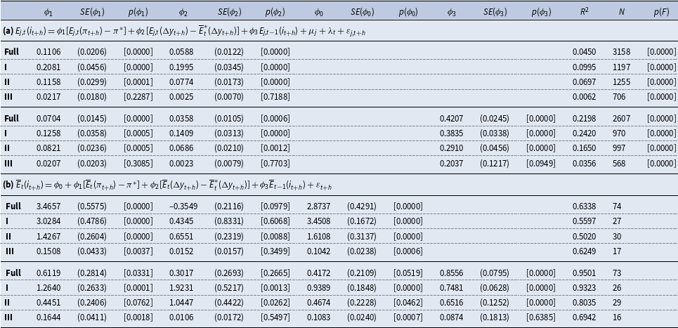
Panel (a) in Table 1 reports estimation results for equation (2) with and without the lagged policy rate forecast for the full sample period from 2002Q1 to 2020Q2 (Full) as well as three sub-sample periods: 2002Q1 to 2008Q3 (I), 2008Q4 to 2016Q1 (II), and 2016Q2 to 2020Q2 (III). The first sub-sample period is considered as the pre-crisis period and the collapse of Lehman Brothers in September 15, 2008 is chosen as the start of the crisis. The second sub-sample period is roughly defined as crisis period, which includes the global financial crisis and also the following European debt crisis. Finally, the third sample period is simply classified as the zero lower bound (ZLB) period and includes the time frame with a MRO rate of zero. The main findings are as follows. First, except for the ZLB period professional forecasters seem to follow the Taylor rule as their policy rate expectations are positively affected by their expectations regarding both deviations of inflation from its target and of GDP growth from its potential and both coefficients (i.e.
 $\phi_1$
and
 $\phi_2$
) are significantly different from zero. In the latest period, this connection unsurprisingly disappears due to the zero interest rate policy of the ECB supported by announcements within its forward guidance strategy. Therefore, during the ZLB period, the ECB has not changed their policy rate due to variations in inflation and/or output gap and professionals have expected this policy rate path. Therefore, both coefficients are not significantly different from zero in the latest period. Second, the connection of policy rate expectations of professionals to their expectations regarding inflation and output gap has lowered over time, which is indicated by the magnitude of the coefficients and by the
 $R^2$
. Third, the one-quarter lagged policy rate forecast also turns out to be (highly) significant and confirms an interest rate smoothing in the expectation building mechanism.
Panel Taylor rule estimations

Note: The table reports panel data estimation results for the regression models given above for a horizon of
 $h=4$
quarters-ahead for the period from 2002Q1 to 2020Q2 (Full) as well as three sub-sample periods: 2002Q1 to 2008Q3 (I), 2008Q4 to 2016Q1 (II) and 2016Q2 to 2020Q2 (III). Panel (a) reports fixed-effects regression results exploiting the cross-sectional variation across individual forecasters and Panel (b) provides time series estimation results for the means across individual forecasters.
 $E_{j,t}(.)$
denotes the forecast for the period
 $t+h$
made in t by forecaster j and
 $\bar{E}_{t}(.)$
gives its mean across forecasters,
 $i_{t}$
stands for the ECB policy rate,
 $\pi_t$
represents Euro Area (EA) inflation and
 $\Delta y_{t}$
denotes EA GDP growth.
 $\pi^*$
stands for the inflation target rate of the ECB and equals 2% and
 $\bar{E}_{t}^*(\Delta y_{t+h})$
represents EA potential GDP growth measured by Hodrick-Prescott-filtered GDP growth mean forecasts across forecasters.
 $SE(.)$
denotes heteroskedasticity and autocorrelation consistent (HAC) standard errors following Andrews (Reference Andrews1991) and
 $p(.)$
gives the corresponding p-values. N reports the sample size and p(F) stands for the p-value for the F-statistic testing the significance of individual and time fixed effects
 $\mu_j$
and
 $\lambda_t$
. The
 $R^2$
for the panel models reported in Panel (a) gives the incremental
 $R^2$
excluding the fraction attributed to individual and time fixed effects
 $\mu_j$
and
 $\lambda_t$
, which explain most of the variation in
 $E_{j,t}(i_{t+h})$
.
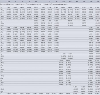
As a robustness check, Panel (b) in Table 1 also reports coefficient estimates for the means across individual forecasters solely focusing on the variation over time. These results generally confirm our previous findings but show much larger coefficient estimates due to aggregation across forecasters. We also find that average policy rate expectations can significantly be explained by inflation expectations and that this association decreases over time. Output gap expectations are especially significant within the crisis period, for which professionals expected the ECB to lower its policy rate to stimulate economic activity and to fight against the recession. To check for robustness, Table 2 provides additional estimation results including several types of location shifts, which account for quarterly periodicity in the forecasts, for decisions of the ECB to change the policy rate and for further location shifts endogenously determined by the split-sample algorithm approach outlined by Castle and Hendry (Reference Castle and Hendry2019), which basically selects all possible location shift dates that turn out to be significant at the 5% level. Overall, the estimates of the coefficients for the expected inflation and output gap do not differ considerably compared to the initial findings reported in Panel (b) in Table 1. Therefore, our main findings seem not to be sensitive to the inclusion of different types of location shifts.Footnote 5
Robustness of mean Taylor rule estimations

Note: The table reports time series estimation results for the means across individual forecasters using the regression model given above for a horizon of
 $h=4$
quarters-ahead for the period from 2002Q1 to 2020Q2 (Full) as well as three sub-sample periods: 2002Q1 to 2008Q3 (I), 2008Q4 to 2016Q1 (II) and 2016Q2 to 2020Q2 (III).
 $\bar{E}_{t}(.)$
denotes the mean forecast across forecasters for the period
 $t+h$
made in t,
 $i_{t}$
stands for the ECB policy rate,
 $\pi_t$
represents Euro Area (EA) inflation and
 $\Delta y_{t}$
denotes EA GDP growth.
 $\pi^*$
stands for the inflation target rate of the ECB and equals 2% and
 $\bar{E}_{t}^*(\Delta y_{t+h})$
represents EA potential GDP growth measured by Hodrick-Prescott-filtered GDP growth mean forecasts across forecasters.
 $\text{Q}k_t$
with
 $k=1,2,3,4$
stands for quarterly dummy variables taking a value of 1 in quarter k, and 0 otherwise.
 $\text{I}k_t$
with
 $k=1,\ldots,5$
represent location shifts
 ${I}(t\leq s)=1$
for all quarters up to s, and 0 otherwise, for the quarters s: 2003Q1, 2006Q2, 2009Q1, 2012Q1 and 2014Q2.
 $\text{Decision}_t$
defines a binary variable equal to 1, if the Governing Council of the ECB made the decision to change its policy rate
 $i_t$
in the quarter prior to the forecast made in t but after the last forecast in
 $t - 1$
, and 0 otherwise.
 $SE(.)$
denotes heteroskedasticity and autocorrelation consistent (HAC) standard errors following Andrews (Reference Andrews1991) and
 $p(.)$
gives the corresponding p-values.
 $\bar{R}^2$
provides the adjusted
 $R^2$
.
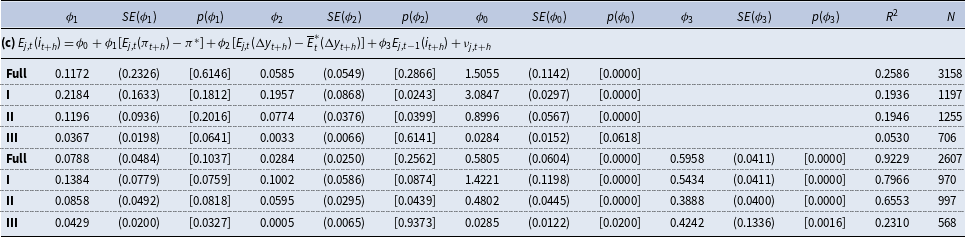
As an additional robustness check for the fixed-effect model estimation results reported in Panel (a) in Table 1, Table 3 provides random effects estimation results.Footnote 6 The coefficients are all very close to the fixed-effects estimates reported in Panel (a) in Table 1. Solely the coefficient estimate of the lagged MRO rate forecast is remarkably higher compared to the fixed-effects model. The significance of the coefficients is diminished, especially for the full sample period specifications. However, the expected inflation gap turns out to be significant even in the zero lower bound period in contrast to the fixed-effects estimates. The next section provides an additional robustness check.
Random effects Taylor rule estimations

Note: The table reports panel data estimation results for the regression models given above for a horizon of
 $h = 4$
quarters-ahead for the period from 2002Q1 to 2020Q2 (Full) as well as three sub-sample periods: 2002Q1 to 2008Q3 (I), 2008Q4 to 2016Q1 (II) and 2016Q2 to 2020Q2 (III). It accompanies Table 1 and adds Panel (c), which reports random effects regression results.
 $E_{j,t}(.)$
denotes the forecast for the period
 $t + h$
made in t by forecaster j and
 $\bar{E}_{t}(.)$
gives its mean across forecasters,
 $i_{t}$
stands for the ECB policy rate,
 $\pi_t$
represents Euro Area (EA) inflation and
 $\Delta y_{t}$
denotes EA GDP growth.
 $\pi^*$
stands for the inflation target rate of the ECB and equals 2% and
 $\bar{E}_{t}^*(\Delta y_{t+h})$
represents EA potential GDP growth measured by Hodrick-Prescott-filtered GDP growth mean forecasts across forecasters.
 $SE(.)$
denotes heteroskedasticity and autocorrelation consistent (HAC) standard errors following Andrews (Reference Andrews1991) and
 $p(.)$
gives the corresponding p-values. N reports the sample size.
3.2 Bias correction
Dynamic fixed-effects models as given by equation (2) are well-known to be subject to the so-called Nickell (Reference Nickell1981) bias. In order to cope with that we also rely on the Bayesian orthogonal reparameterization approach proposed by Lancaster (Reference Lancaster2002). This approach has several benefits compared to other frameworks that are able to eliminate the Nickell (Reference Nickell1981) bias in dynamic fixed-effects models such as, for example, different generalized method of moments (GMM) estimators (Arellano and Bond, Reference Arellano and Bond1991; Blundell and Bond, Reference Blundell and Bond1998), which often appear to be inefficient and also assume the reliability of lags of the left-hand side as instruments and/or require further instruments. The approach proposed by Lancaster (Reference Lancaster2002) is a likelihood-based estimator, which relies on a reparameterization of the individual fixed effects such that these are information orthogonal with all other parameters within the model. This basically means that the slope of the log-likelihood with respect to the individual fixed effects is independent of the slope of the log-likelihood with respect to all other parameters within the model. This approach involves a Bayesian estimation strategy, for which we directly refer to Lancaster (Reference Lancaster2002) and which is carried out with 10,000 Monte Carlo iterations to estimate the posterior distribution. Then parameter estimates are derived as posterior medians and inference is conducted based on credible intervals as quantiles of the posterior.
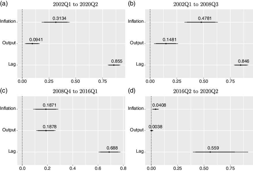
Coefficient estimates and credible intervals.
The plots show parameter estimates and credible intervals based on the dynamic panel model with fixed effects provided in equation (2) using the orthogonal reparameterization approach proposed by Lancaster (Reference Lancaster2002) to eliminate the Nickell (Reference Nickell1981) bias for the full sample period and three sub-sample periods. The parameter estimates are given by the posterior medians and are shown by the black dots. The thin (thick) horizontal lines provide the 95% (90%) credible intervals. The labels Inflation, Output and Lag in the plots refer to estimates of the following coefficients:
 $\phi_{1}$
,
 $\phi_{2}$
, and
 $\phi_{3}$
provided in equation (2).

Figure 3 provides parameter estimates and credible intervals based on the dynamic panel model with fixed effects provided in equation (2) using this orthogonal reparameterization approach for the full sample period and three sub-sample periods. The parameter estimates for
 $\phi_i$
for
 $i=1,2,3$
are shown by the black dots together with the 95% (90%) credible intervals represented by thin (thick) horizontal lines. Overall, the parameter estimates generally confirm the finding that professionals seem to follow the Taylor rule when forming their expectations as the coefficients related to inflation and output gap expectations are significantly positive in (nearly) all cases as the credible intervals do not cover zero. Solely for the ZLB period, the parameter estimates are close to zero, although the coefficient for inflation gap expectations is still significantly different from zero. Therefore, generally Figure 3 confirms our findings provided in Table 1 but it also shows that the coefficient estimates are larger compared to the ones reported in Panel (a) of Table 1 in (nearly) all cases. The latter indicates a potential Nickell (Reference Nickell1981) bias in the estimates provided in Table 1, Panel (a). However, this bias is clearly negative as it turns out in parameter estimates that are too small. This can be seen as evidence for the robustness of the results as the bias-corrected estimates are even more in favor of the finding that professionals believe in the Taylor rule concept.
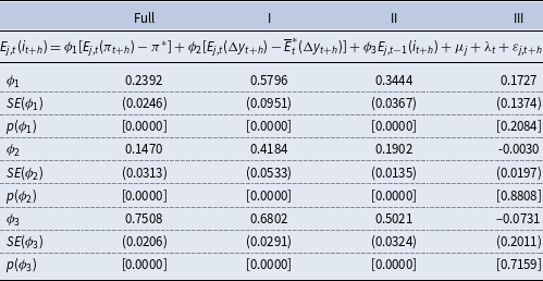
For comparison, Table 4 also reports results for the Arellano and Bond (Reference Arellano and Bond1991) estimator. As can be seen, the coefficient estimates are also larger compared to the ones reported in Panel (a) of Table 1 and roughly similar to the ones provided by the Lancaster (Reference Lancaster2002) approach, which additionally confirms the robustness of our findings. The next section also tests this hypothesis for each individual forecaster and checks the stability of this finding over time.
Arellano-Bond estimation results

Note: The table reports dynamic panel data Arellano and Bond (Reference Arellano and Bond1991) GMM estimation results for the regression model given above for a horizon of
 $ h = 4$
quarters-ahead for the period from 2002Q1 to 2020Q2 (Full) as well as three sub-sample periods: 2002Q1 to 2008Q3 (I), 2008Q4 to 2016Q1 (II) and 2016Q2 to 2020Q2 (III).
 $ E_{j,t}(.)$
denotes the forecast for the period
 $ t + h$
made in t by forecaster j,
 $ i_{t}$
stands for the ECB policy rate,
 $ \pi_t$
represents Euro Area (EA) inflation and
 $ \Delta y_{t}$
denotes EA GDP growth.
 $ \pi^*$
stands for the inflation target rate of the ECB and equals 2% and
 $ \bar{E}_{t}^*(\Delta y_{t+h})$
represents EA potential GDP growth measured by Hodrick-Prescott-filtered GDP growth mean forecasts across forecasters.
 $ SE(.)$
denotes heteroskedasticity and autocorrelation consistent (HAC) standard errors following Windmeijer (Reference Windmeijer2005) and
 $ p(.)$
gives the corresponding p-values.
3.3 Heterogeneity of parameter estimates
Figure 4 also illustrates Taylor rule coefficient estimates for each individual forecaster j and therefore exploits the cross-sectional variation across forecasters in the data.Footnote 7 The relationship between MRO rate and inflation expectations becomes at least evident for 35% of the forecasters, for which we find a significantly positive coefficient over the entire sample period as indicated by a red dot in Panel (a) in Figure 4. Most of the individual estimates of
 $\phi_{j,1}$
range between 0.1 and 0.6 while the fixed-effects regression model estimates range between 0.02 and 0.21 across the different specifications (see Panel (a) in Table 1). First of all, the ranges of coefficient estimates overlap and therefore confirm the robustness of the fixed-effects regression estimates. Second, they tend to be a bit higher on the individual level, which is also supported by the Taylor rule relationship and which also underlines the relevance to account for heterogeneity among forecasters. In line with the Taylor principle, the plot also displays one coefficient estimate larger than unity. Third, the individual coefficient estimates are more in line with the bias corrected dynamic panel model estimates provided in Figure 3 and Table 4.
Individual Taylor rule estimations.
The plots show individual ordinary least squares (OLS) estimation results for the following regression model
 \begin{equation*} E_{j,t}(i_{t+h})=\phi_{j,1}[E_{j,t}(\pi_{t+h})-\pi^*]+\phi_{j,2}[E_{j,t}(\Delta y_{t+h})-\overline{E}_{t}^*(\Delta y_{t+h})]+\sum_{k=1}^4\gamma_{j,k}\text{Q}k_t+\sum_{k=1}^5\delta_{j,k}\text{I}k_t+\varepsilon_{j,t+h}, \end{equation*}
where
 $E_{j,t}(.)$
denotes the forecast for the period
 $t+h$
made in t by forecaster j,
 $i_{t}$
stands for the ECB policy rate,
 $\pi_t$
represents Euro Area (EA) inflation and
 $\Delta y_{t}$
denotes EA GDP growth.
 $\pi^*$
stands for the inflation target rate of the ECB and equals 2% and
 $\overline{E}_{t}^*(\Delta y_{t+h})$
represents EA potential GDP growth measured by Hodrick-Prescott- filtered GDP growth mean forecasts across forecasters.
 $\text{Q}k_t$
represents quarterly dummy variables and
 $\text{I}k_t$
stands for location shifts both defined in Table 2. Panels (a) and (b) illustrate OLS estimates for
 $\phi_{j,1}$
and
 $\phi_{j,2}$
, respectively, for individual forecasters and a horizon of
 $h=4$
quarters-ahead plotted against the
 $R^2$
of the regression. Red dots represent coefficient estimates, which are significantly different from zero at a 5% level.

The association of MRO rate expectations with output gap expectations is less clear but also provides significantly positive coefficients for several forecasters as shown in Panel (b). For
 $\phi_{j,2}$
individual coefficient estimates mostly range between –0.1 and 0.3 while the corresponding fixed-effects regression model estimates range between 0.02 and 0.12 (see Panel (a) in Table 1), which also supports the robustness of the panel regression results.
To further account for variation over time, Figure 5 also provides cross-sectional Taylor rule regressions for each quarter of our sample period and supports our finding mentioned above that professionals made their forecasts roughly in line with the Taylor rule until the start of the ZLB period. This is indicated by (significantly) positive coefficients for inflation and GDP growth gap expectations as shown in Panels (a) and (b), although these also vary over time. The range of coefficient estimates is similar to the one for individual time series and panel fixed effect estimates discussed above.
Cross-sectional Taylor rule regressions over time.
The plots show individual ordinary least squares (OLS) estimation results for the following regression model
 \begin{equation*} E_{j,t}(i_{t+h})=\phi_{t,0}+\phi_{t,1}[E_{j,t}(\pi_{t+h})-\pi^*]+\phi_{t,2}[E_{j,t}(\Delta y_{t+h})-\overline{E}_{t}^*(\Delta y_{t+h})]+\varepsilon_{j,t+h}, \end{equation*}
where
 $E_{j,t}(.)$
denotes the forecast for the period
 $t+h$
made in t by forecaster j,
 $i_{t}$
stands for the ECB policy rate,
 $\pi_t$
represents Euro Area (EA) inflation and
 $\Delta y_{t}$
denotes EA GDP growth.
 $\pi^*$
stands for the inflation target rate of the ECB and equals 2% and
 $\overline{E}_{t}^*(\Delta y_{t+h})$
represents EA potential GDP growth measured by Hodrick-Prescott-filtered GDP growth mean forecasts across forecasters. Panels (a) and (b) illustrate OLS estimates for
 $\phi_{t,1}$
and
 $\phi_{t,2}$
, respectively, plotted over time and a horizon of
 $h=4$
quarters-ahead. Panels (c) and (d) report the
 $R^2$
of the regressions and the number of observations (n), respectively. Red dots represent coefficient estimates, which are significantly different from zero at a 5% level. Two values during the ZLB period are missing due to no variation in the left-hand side variable as all forecasters expected a policy rate of zero within these two periods.

3.4 Disagreement among forecasters
When assuming that professionals believe (at least to some extent) in the concept of the Taylor rule, then the cross-sectional variation of our data set can be further exploited to study if there is also a relationship in the disagreement among forecasters between the policy rate, inflation, and GDP growth (see also Dräger and Lamla, Reference Dräger and Lamla2017). The theoretical foundation for this relationship is provided by Bauer and Neuenkirch (Reference Bauer and Neuenkirch2017), who propose a forward-looking Taylor rule augmented by forecasters’ disagreement regarding inflation and GDP growth which they interpret as proxies for uncertainty. If professionals believe that the central bank sets its policy rate in response to uncertainty regarding inflation and/or GDP growth and if we consider the disagreement among forecasters as a proxy for uncertainty,Footnote 8 then we would also expect to find a relation between forecasters’ disagreement regarding the policy rate and both macro variables.
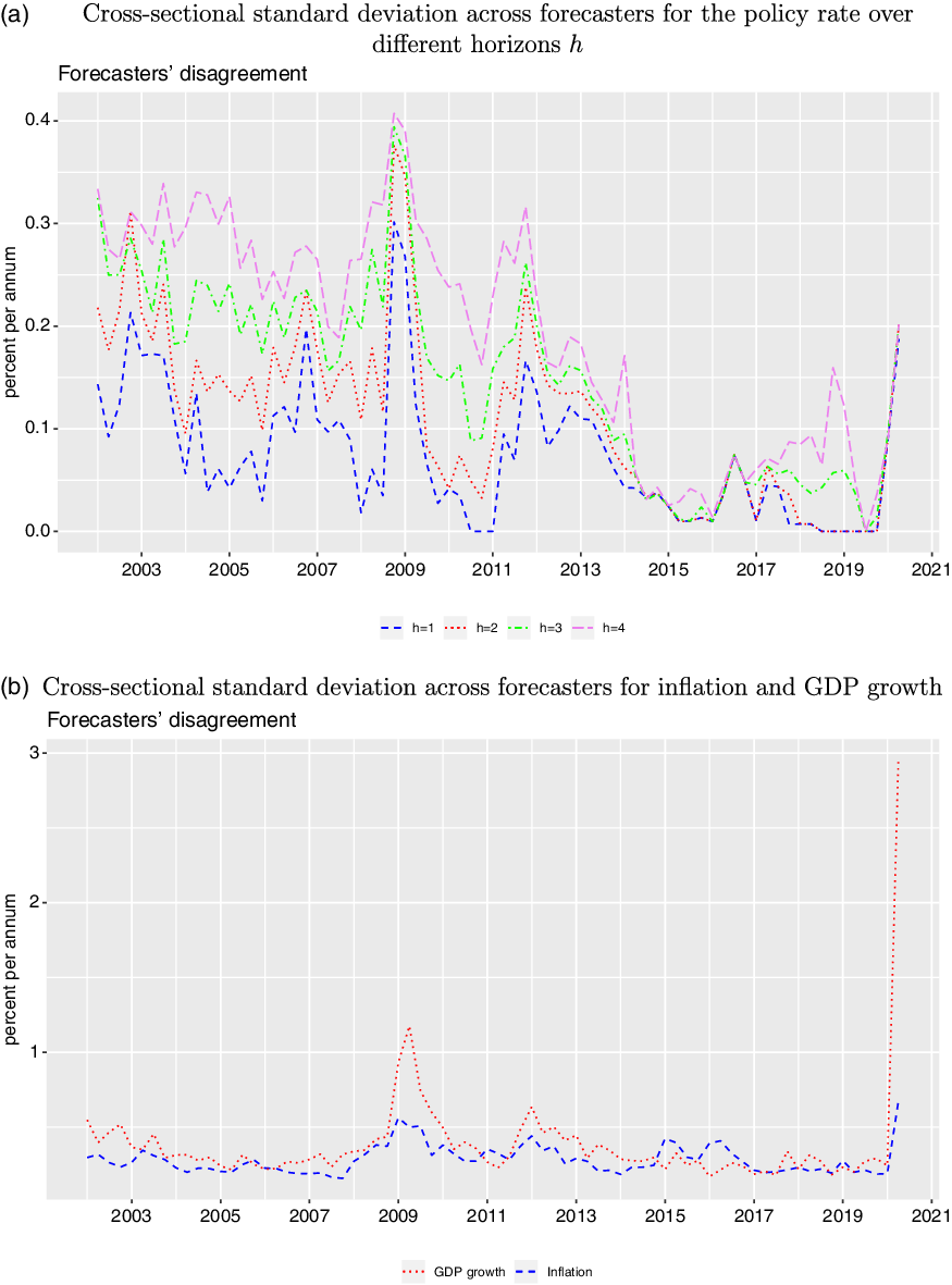
Therefore, as a next step, we have also computed the cross-sectional standard deviation across forecasters for the forecasts regarding all three variables as a measure of disagreement among professional forecasters. Panel (a) in Figure 6 displays this disagreement measure for policy rate forecasts across different forecast horizons h and it becomes clear that disagreement increases with the horizons, peaks around the period of the global financial crisis and has substantially decreased in latest ZLB period. Panel (b) in Figure 6 also provides disagreement among forecasters for 1-year-ahead forecasts for inflation and GDP growth. The general level of disagreement is higher for inflation and GDP growth compared to the policy rate and the most pronounced spikes become evident around the global financial crisis and the corona crisis in the latest period of our sample.
Forecasters’ disagreement.
The plot shows quarterly disagreement among forecasters for the ECB policy rate, inflation and GDP growth measured as the cross-sectional standard deviation across forecasters (in percent per annum) for the period from 2002Q1 to 2020Q2 and for the forecast horizon of four-quarters-ahead. The data has been taken from the ECB survey of professional forecasters (SPF).

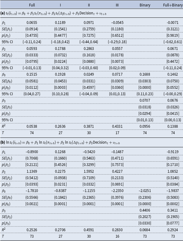
Finally, we estimate the following regression model to examine the Taylor rule-based relationship among the disagreement measures:
 \begin{equation}s_{t}(i_{t+h})=\beta_0+\beta_1s_{t}(\pi_{t+h})+\beta_2s_{t}(\Delta y_{t+h})+\nu_{t+h},\end{equation}
where
 $s_{t}(.)$
denotes the cross-sectional standard deviation across forecasters regarding forecasts made in t.Footnote 9 Panel (a) in Table 5 reports the corresponding coefficient estimates for the full sample period and the three sub-samples already considered above. Our findings indicate that forecasters’ disagreement regarding the policy rate appears not to be attached to disagreement regarding inflation since the corresponding
 $\beta_1$
coefficient is clearly insignificant for all sample periods. This result contrasts the finding of Dräger and Lamla (Reference Dräger and Lamla2017), who find that disagreement regarding the interest rate is dominated by disagreement on future inflation relying on US survey data. However, the disagreement among forecasters regarding the policy rate seems to be an increasing function of the disagreement regarding GDP growth as
 $\beta_2$
is significantly different from zero at least at the 10% level in all four cases. In a final setting we also augment the regression model provided above by a dummy variable, which takes a value of 1, if the Governing Council of the ECB made the decision to change its policy rate
 $i_t$
in the quarter prior to the forecast made in t but after the last forecast in
 $t-1$
, and 0 otherwise. This dummy variable can be seen as a very simply proxy for a monetary policy shock. When controlling for periods marked by Governing Council decisions to change the policy rate, the significant relation mentioned above disappears completely and shows that forecasts of professionals are mainly attached to the current path of the policy rate. According to our findings, the disagreement regarding the policy rate significantly increases if the policy rate has been changed in the current quarter. This finding either might be explained by forecasters’ uncertainty about the future path of monetary policy, which is amplified by the current policy change, or by the presence of information rigidity as outlined by Coibion and Gorodnichenko (Reference Coibion and Gorodnichenko2015). Following their arguments, the inattention of some forecasters in combination with forecast revisions of other forecasters allows the disagreement among forecasters increase after a shock such as the change in the policy rate.
Forecasters’ disagreement regression results

Note: The table reports ordinary least squares (OLS) estimation results for a regression of quarterly time series of disagreement among forecasters as given above for the forecast horizon h of four-quarters-ahead for the period from 2002Q1 to 2020Q2 (Full) as well as three sub-sample periods: 2002Q1 to 2008Q3 (I), 2008Q4 to 2016Q1 (II) and 2016Q2 to 2020Q2 (III).
 $ s_{t}(.)$
measures forecasters‘ disagreement as the cross-sectional standard deviation across individual forecasts,
 $ i_{t}$
stands for the ECB policy rate,
 $ \pi_t$
represents Euro Area (EA) inflation,
 $ \Delta y_{t}$
denotes EA GDP growth and
 $ \text{Decision}_t$
defines a binary variable equal to 1, if the Governing Council of the ECB made the decision to change its policy rate
 $ i_t$
in the quarter prior to the forecast made in t but after the last forecast in
 $ t - 1$
, and 0 otherwise. Panel (a) provides the estimation results for the baseline model and Panel (b) reports the estimation results for the model in natural logarithms. For the latter, we have lost one observation in the zero lower bound period (III) as in one quarter the disagreement among forecasters is zero and therefore
 $ \ln(0)=-\infty$
.
 $ SE(.)$
denotes heteroskedasticity and autocorrelation consistent (HAC) standard errors following Andrews (Reference Andrews1991),
 $ p(.)$
gives the corresponding p-values, 95% CI represents the corresponding 95% confidence interval and T stands for the number of time series observations used for estimation.
As an additional robustness test, Panel (b) in Table 5 also reports coefficient estimates for the regression model provided in equation (3) in natural logarithms to circumvent any problems that might arise from the non-negativity constraint mentioned in Footnote 9. Overall, the estimation results for the log-specification support our main findings for the baseline model that disagreement regarding inflation is insignificant in all specifications and that disagreement regarding GDP growth is significantly positive in all specifications. The only difference is that disagreement regarding GDP growth stays significant at the 5% level even after controlling for a policy change within the last model specification.
4. Conclusion
This study examines if professional forecasters form their expectations regarding the policy rate of the ECB consistent with the Taylor rule. Overall, our findings suggest that this is the case. When considering variation in expectations across forecasters and over time, it becomes evident that professional forecasters explicitly or implicitly take the Taylor rule as a guideline to form their policy rate expectations as we have found a clearly significant relationship between these forecasts and their individual expectations regarding inflation and output gap. This shows that professionals indeed believe that the ECB reacts to deviations in inflation from its target and output from its potential when setting its policy rate. However, we also find that this connection has weakened over the recent decades and has (nearly) disappeared in the latest ZLB period. This is reasonable due to the fact that the policy rate of the ECB is zero for a relatively long period of time and that the ECB has also enhanced communication of their willingness to maintain this policy in the future. Nevertheless, the variation of MRO forecasts in the cross-section and the results for individual forecasters also show that at least some forecasters still believe in a connection of the policy rate with the inflation rate. In addition, we also find a relationship between forecasters’ disagreement regarding the policy rate of the ECB and disagreement on future GDP growth, which disappears when controlling for monetary policy shocks proxied by changes in the policy rate in the quarter the forecasts are made. Therefore, this study provides useful insights into the expectation building mechanism of professionals and guidelines for calibrating economic models.
Acknowledgments
The author thanks two anonymous reviewers for their valuable comments on a previous draft of the article.
Declaration of interests
The author declares that he has no known competing financial interests or personal relationships that could have appeared to influence the work reported in this article.