



1 Introduction
A detonation is a chemically driven compressible wave. A shock wave at the detonation wave front compresses the explosive material, and the subsequent interaction between energy release associated with chemical reaction and compressible flow evolution provide the dynamics that sustains the detonation wave. For a one-dimensional (1-D) planar detonation wave, the speed of the detonation wave is controlled by the initial explosive state, the reaction enthalpy change between reactants and products and the equation of state properties of the product. The detonation speed does not depend on the spatial details of the reaction zone structure (Fickett & Davis Reference Fickett and Davis1979). The minimum speed of the 1-D detonation wave is known as the Chapman–Jouguet (CJ) speed, where, in a frame travelling with the shock, the flow is sonic at the end of the reaction zone.
In condensed-phase high explosives, the large pressures generated in the detonation lead to lateral yielding of any surrounding material. The associated streamline divergence in the reaction zone causes the lead shock wave to become curved (Bdzil & Stewart Reference Bdzil and Stewart2007). In a majority of high explosive configurations the detonation develops divergent (positive) curvature, such as in a two-dimensional planar or axisymmetric cylindrical geometry (Jackson & Short Reference Jackson and Short2015). In steady flow, the sonic locus, which is also curved, moves from the end of the reaction zone and now lies internal to the reaction zone (figure 1). This cuts off some of the chemical energy that would otherwise drive the detonation shock. Along with the energy required to sustain the lateral flow divergence, the detonation wave speed is lowered from its equivalent 1-D CJ value. The region between the shock and sonic locus is known as the detonation driving zone (DDZ). Its structure controls the detonation wave speed in multi-dimensional steady flows (Bdzil & Stewart Reference Bdzil and Stewart2007).
A schematic of the multi-dimensional structure of a detonation wave in a condensed-phase explosive. The figure is based on figure 10 from Bdzil et al. (Reference Bdzil, Aslam, Henninger and Quirk2003) (with permission of J. B. Bdzil).

In addition to the coupling between chemical reaction and compressible flow in the reaction zone, the impedance properties of an inert confiner surrounding the HE can play a significant role in determining the DDZ structure, and thus the detonation speed. Detonation confinement by solid inert materials of different impedances has been extensively studied (Aslam & Bdzil Reference Aslam and Bdzil2002, Reference Aslam and Bdzil2006; Sharpe & Bdzil Reference Sharpe and Bdzil2006; Bdzil & Stewart Reference Bdzil, Stewart and Zhang2011; Short & Quirk Reference Short and Quirk2018). A qualitative understanding of the multiple types of high explosive (HE) detonation–confiner interaction that are possible can be obtained by the use of oblique wave polar theory. This is conducted in a frame riding with the interaction point of the detonation shock and transmitted confiner wave structure at the HE–confiner material boundary (Bdzil & Stewart Reference Bdzil, Stewart and Zhang2011). From the polar analysis, the effect of the confiner on the DDZ depends primarily on the classification of the flow in the HE at the material boundary as subsonic, sonic or supersonic. If the HE flow at the intersection point is sonic or supersonic, the DDZ does not sense the presence of the confiner. On the other hand, if the flow is subsonic the DDZ is influenced by the material properties of the confiner. Generally, high-impedance materials like copper or steel will result in subsonic flow in the HE at the HE–confiner edge, and thus will have a positive confinement effect (higher detonation speed) for most explosives. Low density plastics like Poly(methyl methacrylate) (PMMA) typically result in sonic flow in the HE at the HE–confiner edge. Consequently, such materials do not influence the DDZ structure. Many other interaction scenarios are possible. A particularly interesting case occurs when the detonation speed in the HE is lower than the sound speed in the confiner material (Sharpe & Bdzil Reference Sharpe and Bdzil2006; Short et al. Reference Short, Quirk, Kiyanda, Jackson, Briggs and Shinas2010). For such cases, there is no oblique wave polar solution in the confiner. The flow in the confiner is subsonic and therefore shockless. In such cases, it is found that a large amplitude pressure disturbance travels in the confiner just ahead of the detonation shock, and significantly influences the development of the DDZ in the HE. This scenario typically occurs with non-ideal explosives like ammonium-nitrate fuel oil (ANFO) used in the mining industry that have a low CJ detonation speed.
What has not received much attention in the literature is the effect on multi-dimensional detonation wave propagation due to porous material confiners, despite its relevance to a number of practical situations. For instance, porous foam materials can be inserted between a high explosive and its confinement (Hill Reference Hill2011) to protect the HE from damage due to thermal and mechanical stimuli. Also, in a majority of explosive mining applications, rock layers surrounding the explosive can possess significant initial porosity (e.g. limestone, sandstone, basalt, coal). The nature of fragmentation of the surrounding rock is known to be significantly influenced by the degree of rock porosity (Ahrens & Gregson Reference Ahrens and Gregson1964; Hagan Reference Hagan1979; Braithwaite & Sharpe Reference Braithwaite, Sharpe, Mohanty and Singh2013). Detonation of high explosives is also used to consolidate initially porous metal, ceramic and composite powders (Prümmer Reference Prümmer and Blazynski1983; Mamalis, Vottea & Manolakos Reference Mamalis, Vottea and Manolakos2001).
The confinement of detonation by porous material confiners has several potentially interesting fluid dynamical properties. Under high pressure loading, for example from pressures generated by a detonating HE, porous materials can compact to a density significantly above the initial density of the porous material. Compaction is also a dynamic relaxation process, i.e. there is a finite length/time scale for the compaction process to transition the initial porous state of the material to its compacted equilibrium state. This sets up an interesting two-way feedback for detonation–porous confiner interactions: the HE detonation is responsible for driving the compaction front in the confiner; in turn, high confiner densities generated during compaction can provide a significant confinement effect on the HE detonation structure, with the compaction relaxation process determining the scale over which this occurs relative to the HE detonation width. The purpose of this article is to explore some of the mechanisms of this interaction. We use basic fluid models for the HE and porous confiner in order to focus on the fluid dynamical aspects of the problem. Both analytical studies and multi-material simulations are conducted to explore the relevant physical phenomena underlying how the dynamics of the compaction process in the porous confiner affects the detonation propagation speed and the structure of the DDZ.
2 Model
For the high pressures induced by detonation, the two materials, high explosive and porous material confiner, will flow. For the purposes of this study, each material is modelled by the Euler equations,
 $$\begin{eqnarray}\frac{\unicode[STIX]{x2202}\unicode[STIX]{x1D70C}}{\unicode[STIX]{x2202}t}+\unicode[STIX]{x1D735}\boldsymbol{\cdot }(\unicode[STIX]{x1D70C}\boldsymbol{u})=0,\quad \frac{\unicode[STIX]{x2202}}{\unicode[STIX]{x2202}t}(\unicode[STIX]{x1D70C}\boldsymbol{u})+\boldsymbol{u}\unicode[STIX]{x1D735}\boldsymbol{\cdot }(\unicode[STIX]{x1D70C}\boldsymbol{u})+\unicode[STIX]{x1D70C}(\boldsymbol{u}\boldsymbol{\cdot }\unicode[STIX]{x1D735})\boldsymbol{u}+\unicode[STIX]{x1D735}p=0,\end{eqnarray}$$
 $$\begin{eqnarray}\frac{\unicode[STIX]{x2202}}{\unicode[STIX]{x2202}t}(\unicode[STIX]{x1D70C}E)+\unicode[STIX]{x1D735}\boldsymbol{\cdot }(\boldsymbol{u}(\unicode[STIX]{x1D70C}E+p))=0,\end{eqnarray}$$
where
 $\unicode[STIX]{x1D70C}$
,
 $\boldsymbol{u}$
,
 $E$
and
 $p$
are the density, velocity vector, specific total energy and pressure respectively. For the two-dimensional planar flow considered in the following, the velocity vector
 $\boldsymbol{u}=(u,v)^{\text{T}}$
.
2.1 High explosive
For the HE, flow equations (2.1) are supplemented by an evolution equation for the reaction progress variable
 $\unicode[STIX]{x1D706}\in [0,1]$
,
 $$\begin{eqnarray}\frac{\unicode[STIX]{x2202}}{\unicode[STIX]{x2202}t}(\unicode[STIX]{x1D70C}\unicode[STIX]{x1D706})+\unicode[STIX]{x1D735}\boldsymbol{\cdot }(\unicode[STIX]{x1D70C}\boldsymbol{u}\unicode[STIX]{x1D706})-\unicode[STIX]{x1D70C}\unicode[STIX]{x1D6EC}=0,\end{eqnarray}$$
where
 $\unicode[STIX]{x1D6EC}$
is a reaction rate. The specific total and internal energies are given by
 $$\begin{eqnarray}E=e(\unicode[STIX]{x1D70C},p,\unicode[STIX]{x1D706})+\frac{1}{2}(u^{2}+v^{2}),\quad e=\frac{p+A}{(\unicode[STIX]{x1D6FE}-1)\unicode[STIX]{x1D70C}}-q\unicode[STIX]{x1D706},\end{eqnarray}$$
where we have assumed a Tait (stiffened-gas) equation-of-state (EOS) model for the internal energy
 $e$
. Also,
 $\unicode[STIX]{x1D6FE}$
is the adiabatic exponent,
 $A$
the stiffened gas constant and
 $q$
the specific reaction enthalpy of the fuel species. The reaction rate model is
 $$\begin{eqnarray}\unicode[STIX]{x1D6EC}=kp(1-\unicode[STIX]{x1D706})^{1/2},\end{eqnarray}$$
where
 $k$
is a rate constant. In the strong shock limit employed here, which assumes the pressure in the ambient HE state is zero,
 $$\begin{eqnarray}q=\frac{D_{CJ}^{2}}{2(\unicode[STIX]{x1D6FE}^{2}-1)}\left(1-\frac{A}{\unicode[STIX]{x1D70C}_{0}D_{CJ}^{2}}\right)^{2},\end{eqnarray}$$
where
 $D_{CJ}$
is the Chapman–Jouguet detonation speed and
 $\unicode[STIX]{x1D70C}_{0}$
is the initial density of the HE. These moderately simple forms of EOS and reaction rate have been shown to successfully capture the primary fluid dynamic mechanisms underlying detonation propagation in problems ranging from confinement effects, stability and reaction-zone structure changes due to detonation shock curvature (Aslam & Bdzil Reference Aslam and Bdzil2002; Sharpe & Braithwaite Reference Sharpe and Braithwaite2005; Short et al.
Reference Short, Anguelova, Aslam, Bdzil, Henrick and Sharpe2008; Li, Mi & Higgins Reference Li, Mi and Higgins2015).
In this article, we examine two HE models. The first, named HE1, is broadly representative of the properties of a high-detonation-speed HE, such as PBX 9502, for which we take
 $$\begin{eqnarray}\left.\begin{array}{@{}c@{}}\displaystyle \unicode[STIX]{x1D70C}_{0}=2~\text{g}~\text{cc}^{-1},\quad A=12.8~\text{GPa},\quad D_{CJ}=8~\text{mm}~\unicode[STIX]{x03BC}\text{s}^{-1},\\ \displaystyle q=3.24~\text{mm}^{2}~\unicode[STIX]{x03BC}\text{s}^{-2},\quad \unicode[STIX]{x1D6FE}=3.\end{array}\right\}\end{eqnarray}$$
The second model, HE2, is broadly representative of the properties of a low-detonation-speed HE, such as ANFO commonly used in mining applications, for which we take
 $$\begin{eqnarray}\left.\begin{array}{@{}c@{}}\displaystyle \unicode[STIX]{x1D70C}_{0}=0.86~\text{g}~\text{cc}^{-1},\quad A=2~\text{GPa},\quad D_{CJ}=4.8~\text{mm}~\unicode[STIX]{x03BC}\text{s}^{-1},\\ \displaystyle q=1.16397~\text{mm}^{2}~\unicode[STIX]{x03BC}\text{s}^{-2},\quad \unicode[STIX]{x1D6FE}=3.\end{array}\right\}\end{eqnarray}$$
2.2 Porous inert
The compaction model we employ is a variant of the commonly used P-
 $\unicode[STIX]{x1D6FC}$
class of models (Davison Reference Davison2008) and contains the essential dynamics that we wish to explore in our study of confinement of detonation by a porous material confiner. These are the dependence of the equilibrium compaction state on the initial solid volume fraction, and a dynamic evolution equation for the solid volume fraction characterized by a relaxation time scale to achieve the compacted equilibrium state. This time scale can be varied relative to the time scale that describes the chemical reaction in the HE. The model used here can be formally derived from the full two-phase continuum flow model formulation of Bdzil et al. (Reference Bdzil, Menikoff, Son, Kapila and Stewart1999) by treating the gas phase as void. We refer to this as the two-phase void limit (2PVL) compaction model. The flow in the porous material is again described by flow equations (2.1) for the porous material pressure
 $(p)$
, density
 $(\unicode[STIX]{x1D70C})$
and velocity
 $(\boldsymbol{u})$
. These are related to the solid-phase state by
 $$\begin{eqnarray}p=\unicode[STIX]{x1D719}_{s}p_{s},\quad \unicode[STIX]{x1D70C}=\unicode[STIX]{x1D719}_{s}\unicode[STIX]{x1D70C}_{s},\quad \boldsymbol{u}=\boldsymbol{u}_{s},\end{eqnarray}$$
where
 $\unicode[STIX]{x1D719}_{s}$
is the volume fraction of solid, and the subscript
 $\{~\}_{s}$
is used to denote the state in the solid phase. The total energy of the porous material is given by
 $$\begin{eqnarray}E=e_{s}(p_{s},\unicode[STIX]{x1D70C}_{s})+B(\unicode[STIX]{x1D719}_{s})+{\textstyle \frac{1}{2}}(u^{2}+v^{2}).\end{eqnarray}$$
The internal energy consists of two additive contributions: the internal energy of the solid as a function of the solid-phase state alone (here we assume an incomplete equation-of-state form
 $e_{s}=e_{s}(p_{s},\unicode[STIX]{x1D70C}_{s})$
) and a term denoted by
 $B(\unicode[STIX]{x1D719}_{s})$
. This latter term is a compaction potential and accounts for the configuration dependent energy in the solid (Bdzil et al.
Reference Bdzil, Menikoff, Son, Kapila and Stewart1999).
The solid volume fraction is determined by an evolutionary compaction law given by
 $$\begin{eqnarray}\frac{\unicode[STIX]{x2202}}{\unicode[STIX]{x2202}t}(\unicode[STIX]{x1D70C}\unicode[STIX]{x1D719}_{s})+\unicode[STIX]{x1D735}\boldsymbol{\cdot }(\unicode[STIX]{x1D70C}\boldsymbol{u}\unicode[STIX]{x1D719}_{s})=\unicode[STIX]{x1D70C}r,\quad r=\frac{\unicode[STIX]{x1D719}_{s}}{\unicode[STIX]{x1D707}_{c}(\unicode[STIX]{x1D719}_{s0})}(1-\unicode[STIX]{x1D719}_{s})(p_{s}-\unicode[STIX]{x1D6FD}).\end{eqnarray}$$
We enforce the assumption
 $r\geqslant 0$
, i.e. the compaction model is not permitted to recover porosity. In the compacted equilibrium state, the solid pressure is balanced by a term
 $\unicode[STIX]{x1D6FD}$
known as the configuration pressure. In the context of this 2PVL compaction model, it can be interpreted as representing the resistance of a granular bed to compaction caused by an applied pressure (Bdzil et al.
Reference Bdzil, Menikoff, Son, Kapila and Stewart1999). The compaction viscosity
 $\unicode[STIX]{x1D707}_{c}$
is a measure of the relaxation time required for the compaction process to achieve equilibrium.
The compaction potential and configuration pressure are related through the equation
 $$\begin{eqnarray}\unicode[STIX]{x1D6FD}=\unicode[STIX]{x1D719}_{s}\unicode[STIX]{x1D70C}_{s}\frac{\text{d}B}{\text{d}\unicode[STIX]{x1D719}_{s}},\end{eqnarray}$$
where, for this study,
 $$\begin{eqnarray}\unicode[STIX]{x1D6FD}=\frac{\unicode[STIX]{x1D70C}_{s}}{\unicode[STIX]{x1D70C}_{s0}}\left[p_{c}(\unicode[STIX]{x1D719}_{s0})\ln \left(\frac{1-\unicode[STIX]{x1D719}_{s0}}{1-\unicode[STIX]{x1D719}_{s}}\right)\right],\end{eqnarray}$$
a choice motivated by that used in Bdzil et al. (Reference Bdzil, Menikoff, Son, Kapila and Stewart1999). The subscript
 $\{~\}_{0}$
notation denotes quantities in the initial material state. The function
 $\unicode[STIX]{x1D6FD}$
contains a logarithmic growth in the limit of full compaction
 $\unicode[STIX]{x1D719}_{s}\rightarrow 1$
, modified by a pressure amplitude term
 $p_{c}$
. We assume that
 $p_{c}$
varies as a function of the initial porosity, i.e.
 $p_{c}=p_{c}(\unicode[STIX]{x1D719}_{s0})$
, where
 $p_{c}$
increases as
 $\unicode[STIX]{x1D719}_{s0}$
increases. This assumption can be related to the property that the more tightly packed the solid matrix is initially, the more difficulty it has rearranging itself to fill the void space. For the purposes of this study, we use a linear form
 $$\begin{eqnarray}p_{c}(\unicode[STIX]{x1D719}_{s0})=a+b\unicode[STIX]{x1D719}_{s0},\end{eqnarray}$$
where
 $a$
and
 $b$
are constants. These parameters are chosen below so that the equilibrium states of the 2PVL compaction model can be fitted to experimental data for our choice of porous material. The corresponding form for
 $B$
is then given by
 $$\begin{eqnarray}B(\unicode[STIX]{x1D719}_{s})=\frac{p_{c}}{\unicode[STIX]{x1D70C}_{s0}}\left[(\ln \unicode[STIX]{x1D719}_{s})\ln \left(\frac{1-\unicode[STIX]{x1D719}_{s0}}{1-\unicode[STIX]{x1D719}_{s}}\right)-\int _{\unicode[STIX]{x1D719}_{s0}}^{\unicode[STIX]{x1D719}_{s}}\frac{\ln \unicode[STIX]{x1D719}_{s}}{1-\unicode[STIX]{x1D719}_{s}}\,\text{d}\unicode[STIX]{x1D719}_{s}\right],\end{eqnarray}$$
where the integral on the right can be written in terms of the dilogarithm function. Note that
 $B(\unicode[STIX]{x1D719}_{s0})=0$
and
 $B(\unicode[STIX]{x1D719}_{s})>0$
, so that the compaction potential results in an increase in the internal energy of the porous material.
For the EOS of the solid, we use a Mie–Gruneisen
 $U_{s}-u_{p}$
form (Davis Reference Davis, Zukas and Walters1997), where
 $$\begin{eqnarray}e_{s}=\frac{c^{2}t^{2}}{2(1-st)^{2}}+\frac{1}{\unicode[STIX]{x1D6E4}_{0}\unicode[STIX]{x1D70C}_{s0}}\left(p_{s}-\frac{\unicode[STIX]{x1D70C}_{s0}c^{2}t}{(1-st)^{2}}\right),\quad t=1-\frac{\unicode[STIX]{x1D70C}_{s0}}{\unicode[STIX]{x1D70C}_{s}}.\end{eqnarray}$$
Here
 $c$
,
 $s$
and
 $\unicode[STIX]{x1D6E4}_{0}$
(Gruneisen gamma) are the
 $U_{s}-u_{p}$
EOS parameters used to fit the EOS for a given solid material to experimental data. The frozen sound speed of the solid phase is
 $$\begin{eqnarray}C_{s}=\left[\frac{\unicode[STIX]{x1D6E4}_{0}\unicode[STIX]{x1D70C}_{s0}p_{s}}{\unicode[STIX]{x1D70C}_{s}^{2}}+\frac{\unicode[STIX]{x1D70C}_{s0}^{2}c^{2}}{\unicode[STIX]{x1D70C}_{s}^{2}(1-st)^{2}}\left(1-\unicode[STIX]{x1D6E4}_{0}t\right)+\frac{2\unicode[STIX]{x1D70C}_{s0}^{2}c^{2}st}{\unicode[STIX]{x1D70C}_{s}^{2}(1-st)^{3}}\left(1-\frac{\unicode[STIX]{x1D6E4}_{0}}{2}t\right)\right]^{1/2}.\end{eqnarray}$$
In the 2PVL porous compaction model, the frozen sound speed of the porous material is equal to the frozen sound speed of the pure solid.
2.2.1 Porous confiner material calibration
For this article, we model the porous confiner material based on cerium oxide
 $(\text{CeO}_{2})$
powder due to the large amount of experimental data measured on compaction states under one-dimensional pressure loading at different initial densities (Fredenburg & Chisolm Reference Fredenburg and Chisolm2014; Fredenburg et al.
Reference Fredenburg, Koller, Coe and Kiyanda2014, Reference Fredenburg, Lang, Coe, Scharff, Dattelbaum and Chisolm2017). Importantly, the Hugoniot state behaviour under shock loading (§ 3) is consistent with most other porous metal powders, and is therefore suited to our primary aim of highlighting the main fluid mechanical elements of HE confinement by porous materials. The
 $U_{s}-u_{p}$
model EOS parameters for solid
 $\text{CeO}_{2}$
(Fredenburg & Chisolm Reference Fredenburg and Chisolm2014) are
 $$\begin{eqnarray}\unicode[STIX]{x1D70C}_{s0}=7.215~\text{g}~\text{cc}^{-1},\quad c=5.635~\text{mm}~\unicode[STIX]{x03BC}\text{s}^{-1},\quad s=1.257,\quad \unicode[STIX]{x1D6E4}_{0}=1.5.\end{eqnarray}$$
2.3 Scaling
To set a reference length scale, we introduce non-dimensional length and time scalings, along with a rescaling of the HE rate constant
 $k$
and compaction viscosity
 $\unicode[STIX]{x1D707}_{c}$
, where
 $$\begin{eqnarray}\tilde{\boldsymbol{x}}=\frac{\boldsymbol{x}}{l_{1/2}},\quad \tilde{t}=\frac{t}{(l_{1/2}/u_{ref})},\quad \bar{k}=kl_{1/2},\quad \bar{\unicode[STIX]{x1D707}}_{c}=\frac{\unicode[STIX]{x1D707}_{c}}{l_{1/2}}.\end{eqnarray}$$
Here
 $l_{1/2}$
is the physical length behind the shock in the steady planar Chapman–Jouguet detonation wave at which half of the reactant has been consumed, while
 $u_{ref}=1~\text{mm}~\unicode[STIX]{x03BC}\text{s}^{-1}$
. The scaled rate constant for HE1 is then
 $\bar{k}\approx 0.05135906~\text{mm}~\unicode[STIX]{x03BC}\text{s}^{-1}~\text{GPa}^{-1}$
, while the rate constant for HE2 is
 $\bar{k}\approx 0.19942118~\text{mm}~\unicode[STIX]{x03BC}\text{s}^{-1}~\text{GPa}^{-1}$
. The magnitude of
 $\bar{\unicode[STIX]{x1D707}}_{c}$
then sets the relaxation length for the compaction process to reach equilibrium relative to the half-reaction-zone length of the CJ detonation wave in the HE.
3 Steady-state compaction wave structure and equilibrium states
Equilibrium states for steady propagating 1-D compaction waves for the 2PVL model defined in § 2.2 for
 $\text{CeO}_{2}$
at different initial porous material densities are calculated by using the constant wave speed
 $(D_{0})$
conservation relations appropriate to the 2PVL model,
 $$\begin{eqnarray}u=D_{0}\left(1-\frac{\unicode[STIX]{x1D70C}_{0}}{\unicode[STIX]{x1D70C}}\right),\quad p=\unicode[STIX]{x1D70C}_{0}D_{0}^{2}\left(1-\frac{\unicode[STIX]{x1D70C}_{0}}{\unicode[STIX]{x1D70C}}\right),\quad e+\frac{1}{2}p\left(\frac{1}{\unicode[STIX]{x1D70C}}-\frac{1}{\unicode[STIX]{x1D70C}_{0}}\right)=0,\end{eqnarray}$$
where
 $e=e_{s}(p_{s},\unicode[STIX]{x1D70C}_{s})+B(\unicode[STIX]{x1D719}_{s})$
, and calculating the state for which
 $$\begin{eqnarray}p_{s}=\unicode[STIX]{x1D6FD}.\end{eqnarray}$$
As stated above, construction of the equilibrium states for the 2PVL model require the specification of configuration pressure (
 $p_{c}$
) parameters
 $a$
and
 $b$
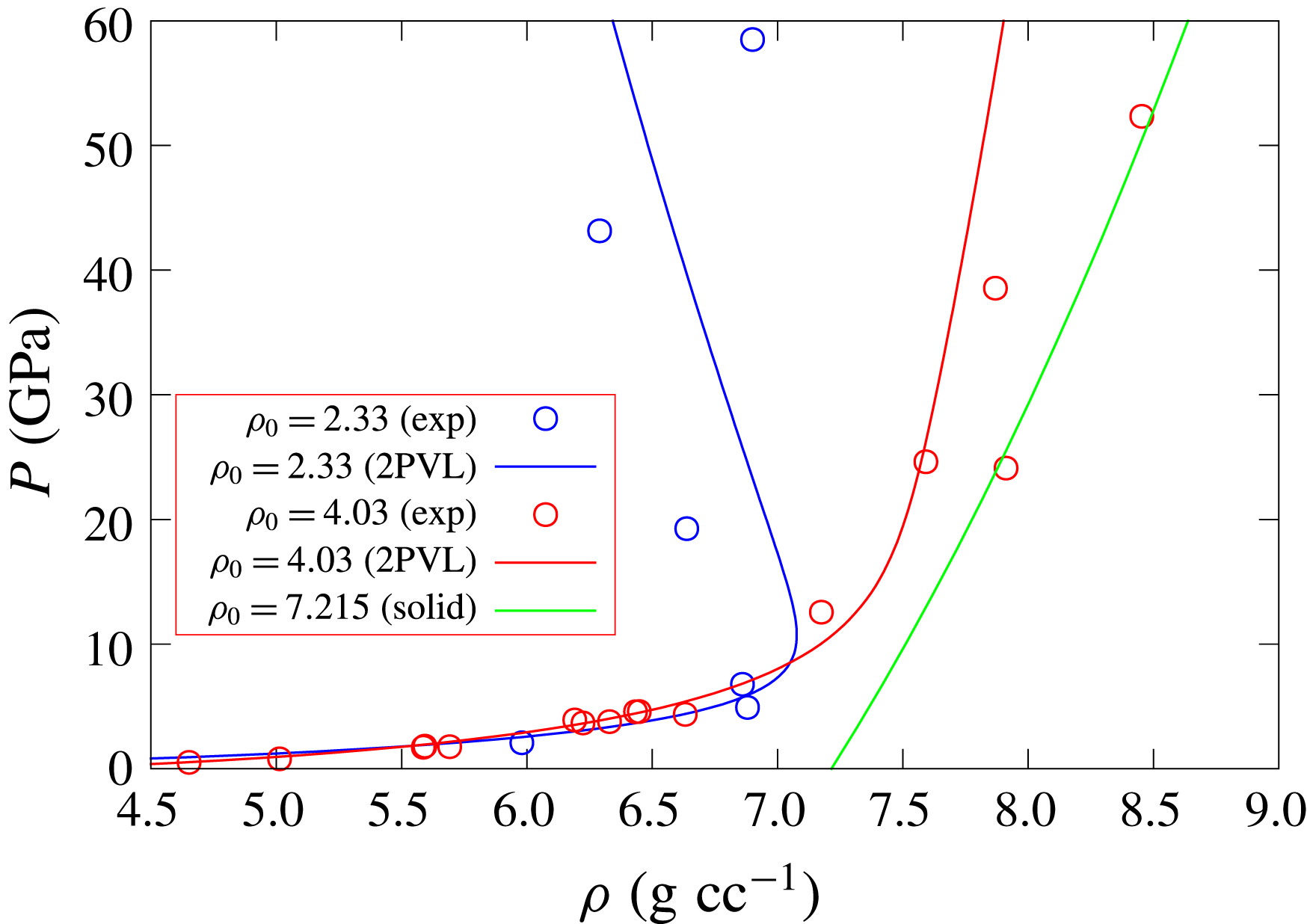
. Figure 2 shows 1-D compaction wave equilibrium states in the pressure–density plane for the 2PVL model for
 $\text{CeO}_{2}$
for the two initial densities
 $\unicode[STIX]{x1D70C}_{0}=4.03~\text{g}~\text{cc}^{-1}\;(\unicode[STIX]{x1D719}_{s0}=0.5586)$
and
 $\unicode[STIX]{x1D70C}_{0}=2.33~\text{g}~\text{cc}^{-1}\;(\unicode[STIX]{x1D719}_{s0}=0.3229)$
at which experimental compaction equilibrium states are available for one-dimensional pressure loaded
 $\text{CeO}_{2}$
powders (Fredenburg & Chisolm Reference Fredenburg and Chisolm2014; Fredenburg et al.
Reference Fredenburg, Koller, Coe and Kiyanda2014, Reference Fredenburg, Lang, Coe, Scharff, Dattelbaum and Chisolm2017). Also shown for comparison is the shock-state Hugoniot for solid
 $\text{CeO}_{2}$
, calculated using (2.16) and (2.18). The parameters
 $a$
and
 $b$
are chosen so that the 2PVL model equilibrium states can reasonably fit the experimental data across the two initial densities, whereupon
 $$\begin{eqnarray}a=0~\text{GPa},\quad b=7~\text{GPa}.\end{eqnarray}$$
Given the large uncertainties in the experimental data especially at higher pressures (Fredenburg & Chisolm Reference Fredenburg and Chisolm2014), and the emphasis of the current paper to highlight the basic fluid mechanics of HE confinement by porous materials, the fit obtained with (3.3) is sufficient for a 2PVL model of porous
 $\text{CeO}_{2}$
. The two Hugoniot curve shapes obtained for
 $\unicode[STIX]{x1D70C}_{0}=4.03$
and
 $2.33~\text{g}~\text{cc}^{-1}$
are typical of those obtained for increasingly porous materials (Zel’dovich & Raizer Reference Zel’dovich and Raizer2002). Their respective
 $P-\unicode[STIX]{x1D70C}$
Hugoniot behaviour, relative to that of the Hugoniot for the solid material, results from the work done and subsequent change in internal energy in compacting the porous material to its equilibrium state, and how this change in internal energy is distributed into pressure and density changes. For sufficiently porous materials, increases in pressure above a threshold value are found to be accompanied by decreases in density of the equilibrated material (Zel’dovich & Raizer Reference Zel’dovich and Raizer2002), as shown for
 $\unicode[STIX]{x1D70C}_{0}=2.33~\text{g}~\text{cc}^{-1}$
.
Compaction wave equilibrium states in the pressure–density plane for 1-D travelling wave solutions of the 2PVL model for
 $\text{CeO}_{2}$
at different initial densities. The green line represents the variation in Hugoniot shock state for solid
 $\text{CeO}_{2}$
. The circles represent equilibrium compaction state experimental data from Fredenburg & Chisolm (Reference Fredenburg and Chisolm2014), Fredenburg et al. (Reference Fredenburg, Koller, Coe and Kiyanda2014, Reference Fredenburg, Lang, Coe, Scharff, Dattelbaum and Chisolm2017).
Variation of the compaction equilibrium pressure and density with initial solid volume fraction for (a) subsonic wave speed
 $D_{0}=3~\text{mm}~\unicode[STIX]{x03BC}\text{s}^{-1}$
and (b) supersonic wave speed
 $D_{0}=7~\text{mm}~\unicode[STIX]{x03BC}\text{s}^{-1}$
.

Figure 3 shows the variation of the 1-D equilibrium pressure and density with initial solid volume fraction for the 2PVL model for two compaction wave speeds (
 $D_{0}=3~\text{mm}~\unicode[STIX]{x03BC}\text{s}^{-1}$
, below the initial sound speed
 $C_{s0}$
, and
 $D_{0}=7~\text{mm}~\unicode[STIX]{x03BC}\text{s}^{-1}$
, above
 $C_{s0}$
). Of particular interest is that the compaction equilibrium pressures and densities increase significantly as
 $\unicode[STIX]{x1D719}_{s0}$
increases, before decreasing as the initial solid volume fraction approaches one. This is again a consequence of how the internal energy change due to the work done in compacting the initial porous material to its equilibrium state is distributed amongst pressure and density changes. For a given wave speed, the internal energy change decreases as
 $\unicode[STIX]{x1D719}_{s0}$
increases along each of the curves shown in figure 3. The equilibrium pressure and density at first increase as the initial material porosity decreases, but for sufficiently low initial porosities, the lower internal energy change leads to lower pressure and density states at equilibrium. This behaviour highlights the possibility that even moderately porous materials may have a non-trivial confinement effect on detonation propagation.
The structure of steady travelling compaction waves corresponding to models similar to the 2PVL model in § 2.2 have been constructed and analysed previously (Powers, Stewart & Krier Reference Powers, Stewart and Krier1989; Short et al.
Reference Short, Fredenburg, Lang, Gambino, Kapila and Schwedeman2015). Compaction waves travelling at speeds
 $D_{0}<C_{s0}$
are subsonic and fully dispersed spatially. Waves travelling at speeds
 $D_{0}>C_{s0}$
are supersonic and led by a shock front, where the solid volume fraction behind the shock is equal to the initial solid volume fraction (i.e.
 $[\unicode[STIX]{x1D719}_{s}]=0$
). Spatially dispersed compaction occurs behind the shock. One-dimensional steady travelling compaction wave solutions for a given
 $D_{0}$
are obtained from the conservation relations (3.1) along with the steady travelling wave form of the solid volume fraction evolution equation (2.11),
 $$\begin{eqnarray}(u-D_{0})\frac{\text{d}\unicode[STIX]{x1D719}_{s}}{\text{d}\tilde{x}}=r,\quad r=\frac{\unicode[STIX]{x1D719}_{s}}{\bar{\unicode[STIX]{x1D707}}_{c}(\unicode[STIX]{x1D719}_{s0})}(1-\unicode[STIX]{x1D719}_{s})(p_{s}-\unicode[STIX]{x1D6FD}).\end{eqnarray}$$
For the subsonic dispersed solutions
 $(D_{0}<C_{s0})$
, we construct asymptotic solutions for the travelling wave solution for
 $\unicode[STIX]{x1D719}_{s}-\unicode[STIX]{x1D719}_{s0}\ll 1$
, and integrate from this construction to the equilibrium solution, where
 $p_{s}=\unicode[STIX]{x1D6FD}$
. For the supersonic shock-led solutions (
 $D_{0}>C_{s0}$
), we first construct the Hugoniot shock state from (3.1) assuming
 $[\unicode[STIX]{x1D719}_{s}]=0$
, i.e.
 $\unicode[STIX]{x1D719}_{s}=\unicode[STIX]{x1D719}_{s0}$
, and then subsequently integrate from this state to the equilibrium state.
Pressure (solid lines) and solid volume fraction (dotted lines) variation in steady compaction wave profiles for the 2PVL model with various choices of compaction viscosity. Shown are the fully dispersed compaction wave profiles for subsonic speeds (a)
 $D_{0}=1~\text{mm}~\unicode[STIX]{x03BC}\text{s}^{-1}$
(with
 $\unicode[STIX]{x1D719}_{s0}=0.3229$
) and (b)
 $D_{0}=3~\text{mm}~\unicode[STIX]{x03BC}\text{s}^{-1}$
(also with
 $\unicode[STIX]{x1D719}_{s0}=0.3229$
), and the shock wave-led compaction wave profile for the supersonic speed (c)
 $D_{0}=7~\text{mm}~\unicode[STIX]{x03BC}\text{s}^{-1}$
(with
 $\unicode[STIX]{x1D719}_{s0}=0.5586$
). The units of the scaled compaction viscosity
 $\bar{\unicode[STIX]{x1D707}}_{c}$
are
 $\text{mm}^{-1}~\unicode[STIX]{x03BC}\text{s}~\text{GPa}$
.

Figure 4 shows the steady wave pressure and solid volume fraction spatial variation for the
 $\text{CeO}_{2}$
2PVL model with various choices of wave speed, initial solid volume fraction and compaction viscosity. We note that experimental data on characteristic time scales to compact the initial porous material to the equilibrium state are limited (Fredenburg & Chisolm Reference Fredenburg and Chisolm2014). The attempts that have been made on
 $\text{CeO}_{2}$
powders indicate that the relaxation times may be faster or comparable to those characteristic of a detonation reaction zone thickness (Fredenburg & Chisolm Reference Fredenburg and Chisolm2014). However, since the diagnostic methods have several limitations, and for the general consideration of other porous materials with different compaction relaxation rates, in this article we will explore the effects of variation in
 $\bar{\unicode[STIX]{x1D707}}_{c}$
on the HE detonation confinement effect. Cases (a) and (b) in figure 4 are for subsonic wave speeds. For sufficiently low speeds (
 $D_{0}=1~\text{mm}~\unicode[STIX]{x03BC}\text{s}^{-1}$
), the equilibrium state is not fully compacted. Increasing the compaction viscosity slows the compaction rate and this spreads the compaction wave out spatially. We note that the relaxation length for the compaction process is relative to the scale that sets the half-reaction-zone length in the CJ detonation wave to one (§ 2.3). In the supersonic case for
 $D_{0}=7~\text{mm}~\unicode[STIX]{x03BC}\text{s}^{-1}$
, figure 4(c), the compaction process is led by a shock wave, where again increases in
 $\bar{\unicode[STIX]{x1D707}}_{c}$
slow the compaction process behind shock.
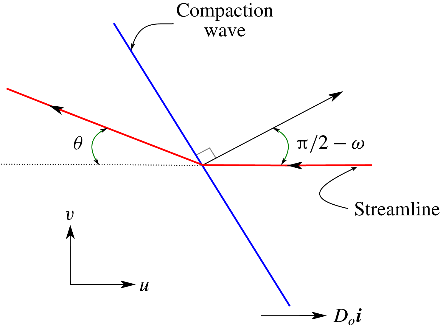
A schematic of the streamline turning due to a compaction wave travelling horizontally with speed
 $D_{0}$
and obliquely turned at an angle
 $\unicode[STIX]{x03C0}/2-\unicode[STIX]{x1D714}$
to the horizontal.
4 Oblique compaction wave polar analysis
An analysis similar to oblique shock polar theory can be used to calculate the equilibrium state of a compaction wave turned at an angle
 $\unicode[STIX]{x03C0}/2-\unicode[STIX]{x1D714}$
to the horizontal and propagating in the horizontal direction with a velocity
 $D_{0}$
. A schematic of the resulting flow turning is shown in figure 5. The streamline turning angle is denoted by
 $\unicode[STIX]{x1D703}$
. Along with the equilibrium condition
 $p_{s}=\unicode[STIX]{x1D6FD}$
(3.2), the following conservation equations, derived from (2.1), can be used to calculate the resulting equilibrium state,
 $$\begin{eqnarray}u_{n}=D_{0}\sin (w)\left(1-\frac{\unicode[STIX]{x1D70C}_{0}}{\unicode[STIX]{x1D70C}}\right),\quad p=\unicode[STIX]{x1D70C}_{0}D_{0}^{2}\sin ^{2}(w)\left(1-\frac{\unicode[STIX]{x1D70C}_{0}}{\unicode[STIX]{x1D70C}}\right),\quad e+\frac{1}{2}p\left(\frac{1}{\unicode[STIX]{x1D70C}}-\frac{1}{\unicode[STIX]{x1D70C}_{0}}\right)=0,\end{eqnarray}$$
where
 $u_{n}$
is the flow speed normal to the compaction wave, with
 $$\begin{eqnarray}u=u_{n}\sin (w),\quad v=u_{n}\cos (w),\end{eqnarray}$$
and
 $e=e_{s}(p_{s},\unicode[STIX]{x1D70C}_{s})+B(\unicode[STIX]{x1D719}_{s})$
. The streamline turning angle is then
 $$\begin{eqnarray}\unicode[STIX]{x1D703}=\arctan \left(\frac{v}{D_{0}-u}\right),\end{eqnarray}$$
while the Mach number of the equilibrium compaction state relative to the wave motion is
 $$\begin{eqnarray}M=\frac{\sqrt{(D_{0}-u)^{2}+v^{2}}}{C_{s}}.\end{eqnarray}$$
Equilibrium states for the 2PVL model behind the obliquely turned compaction wave showing the pressure
 $p$
as a function of streamline turning angle
 $\unicode[STIX]{x1D703}$
and solid volume fraction
 $\unicode[STIX]{x1D719}_{s}$
for various initial solid volume fractions
 $\unicode[STIX]{x1D719}_{s0}$
and for
 $D_{0}=7~\text{mm}~\unicode[STIX]{x03BC}\text{s}^{-1}$
(a,b) and
 $D_{0}=6~\text{mm}~\unicode[STIX]{x03BC}\text{s}^{-1}$
(c,d). The circles indicate
 $\unicode[STIX]{x1D703}$
and
 $\unicode[STIX]{x1D719}_{s}$
corresponding to sonic flow. The shock polars for the solid material are also shown in (a) and (c). The detonation shock polars for the HE model HE1 are shown in (a) and (c), along with the HE Prandtl–Meyer fan states (dashed lines).
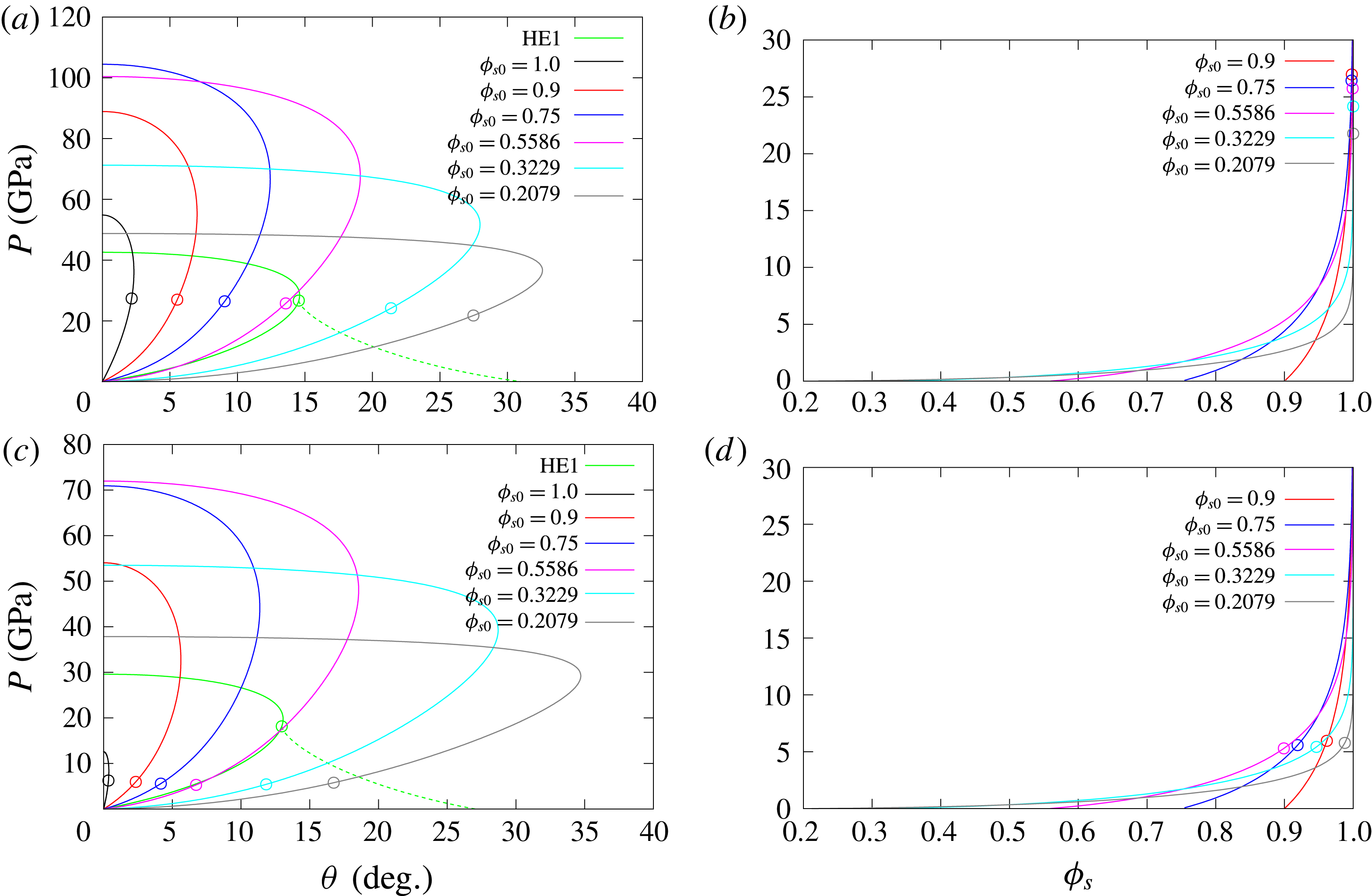
Figure 6 shows the equilibrium states for the 2PVL model behind the obliquely turned compaction wave (pressure
 $p$
as a function of streamline turning angle
 $\unicode[STIX]{x1D703}$
and solid volume fraction
 $\unicode[STIX]{x1D719}_{s}$
) for various initial solid volume fractions (
 $\unicode[STIX]{x1D719}_{s0}$
) and for the compaction wave speeds
 $D_{0}=7$
and
 $D_{0}=6~\text{mm}~\unicode[STIX]{x03BC}\text{s}^{-1}$
. Also shown for each
 $D_{0}$
is the equilibrium state solid volume fraction
 $\unicode[STIX]{x1D719}_{s}$
. These cases have
 $D_{0}$
greater than
 $C_{s0}$
, and consequently the shock polar solutions for the solid material
 $(\unicode[STIX]{x1D719}_{s0}=1)$
can also be calculated. The turning angle and solid volume fraction corresponding to equilibrium flow that is sonic for each
 $\unicode[STIX]{x1D719}_{s0}$
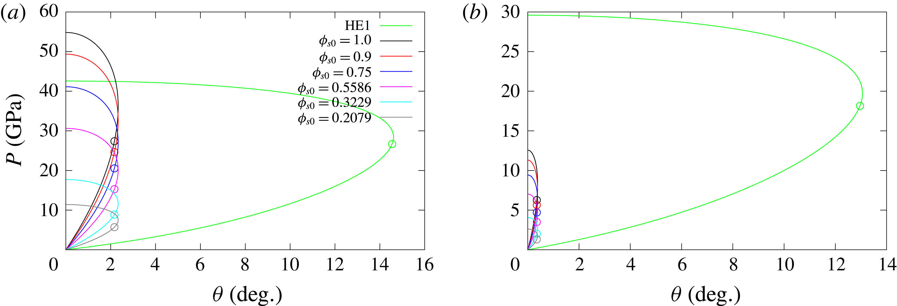
is also highlighted. Polar solutions for pressures above the sonic solution are subsonic, while those below are supersonic. While the shock polar solutions for the solid material in (a) and (c) have a small maximum streamline turning angle, one of the most striking features of the equilibrium polar solutions for initially porous materials is the large increase in maximum streamline turning angle that occurs as
 $\unicode[STIX]{x1D719}_{s0}$
decreases. Also, the pressures in the oblique wave required to drive the porous material to a fully compacted state (figure 6
b,d) are moderately large (
 ${\approx}20~\text{GPa}$
), except for the two lowest
 $\unicode[STIX]{x1D719}_{s0}$
shown.
The detonation shock polar solution for HE model HE1 is additionally shown in figure 6(a,c), and this permits a discussion of the types of detonation–porous confiner flow interactions that we might expect to observe based solely on oblique wave theory. For
 $D_{0}=7~\text{mm}~\unicode[STIX]{x03BC}\text{s}^{-1}$
, the polar curve for the solid confiner has one direct match point with the detonation shock polar curve, which is known as a strong interaction solution (Aslam & Bdzil Reference Aslam and Bdzil2006; Sharpe & Bdzil Reference Sharpe and Bdzil2006). With decreasing
 $D_{0}$
, the solid confiner polar moves inside the HE detonation shock polar (e.g. as seen for
 $D_{0}=6~\text{mm}~\unicode[STIX]{x03BC}\text{s}^{-1}$
), and no direct match point exists. However, the equilibrium compaction state polar solutions for the porous material shown with
 $\unicode[STIX]{x1D719}_{s0}\geqslant 0.5586$
each have one direct match point with the detonation shock polar solution (figure 6
a). The existence of these high pressure direct match points is a consequence of the compaction wave behaviour seen in figure 3, where the pressures generated at the equilibrium compaction state for a range of initial solid volume fractions at a fixed
 $D_{0}$
are above those for the initially solid material. The aforementioned polar intersection points occur on the subsonic branches of both the detonation and compaction polars, and, as such, we might expect that the detonation driving zone structure (§ 1) will be influenced both by the properties and thickness of the confiner. At these strong match points, the equilibrium state is essentially fully compacted (figure 6
b). Additional possible match points for this range of initial solid volume fractions are through a Prandtl–Meyer (PM) fan that extends from the equilibrium state polar sonic point to the supersonic branch of the detonation shock polar. For
 $\unicode[STIX]{x1D719}_{s0}=0.3229$
and
 $\unicode[STIX]{x1D719}_{s0}=0.2079$
, the only match point is through a PM fan originating from the sonic point of the detonation shock polar to the compaction wave equilibrium polar. These are known as weakly confined cases (Aslam & Bdzil Reference Aslam and Bdzil2006; Sharpe & Bdzil Reference Sharpe and Bdzil2006). Consequently, for these initial solid volume fractions, the porous material should not provide any confinement on the detonation propagation. However, even moderately porous confiners with at least
 $\unicode[STIX]{x1D719}_{s0}\geqslant 0.5586$
could be expected to provide strong confinement on the detonation based on the polar analysis. A similar polar interaction description applies for
 $D_{0}=6~\text{mm}~\unicode[STIX]{x03BC}\text{s}^{-1}$
. In this case, the shock polar for the solid confiner has a small maximum pressure amplitude and small maximum streamline turning angle since
 $D_{0}$
is approaching
 $C_{s0}$
. Also, sonic flow for
 $D_{0}=6~\text{mm}~\unicode[STIX]{x03BC}\text{s}^{-1}$
for each of the
 $\unicode[STIX]{x1D719}_{s0}$
shown now occurs in partially compacted equilibrium states. Direct match solutions between the equilibrium compaction wave polars and detonation shock polar occur for
 $\unicode[STIX]{x1D719}_{s0}>0.5586$
, at least up to
 $\unicode[STIX]{x1D719}_{s0}=0.9$
, where the flow is subsonic on both the detonation shock and compaction equilibrium polars. For these strong interaction points, the equilibrium state is again almost fully compacted.
As for figure 6 but with (a,b)
 $D_{0}=4~\text{mm}~\unicode[STIX]{x03BC}\text{s}^{-1}$
and (c,d)
 $D_{0}=2~\text{mm}~\unicode[STIX]{x03BC}\text{s}^{-1}$
. The detonation shock polars for the HE model, HE2, are shown in (a) and (c).
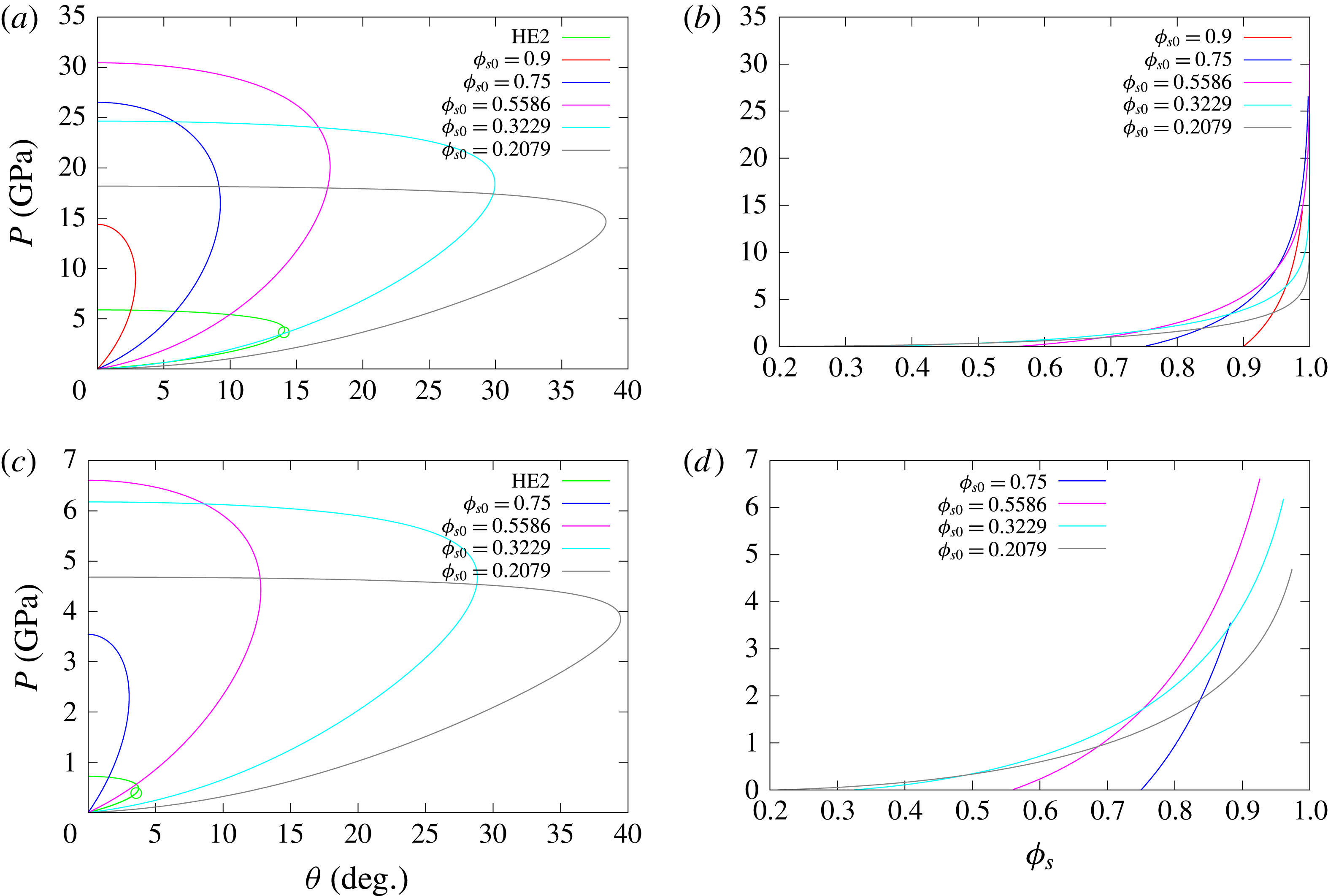
Figure 7 shows the compaction equilibrium state polar solutions for
 $D_{0}=4$
and
 $D_{0}=2~\text{mm}~\unicode[STIX]{x03BC}\text{s}^{-1}$
, relevant to the oblique compaction wave being driven by a low-speed detonation. Here, the compaction wave speeds are slower than the sound speed
 $C_{s0}$
and consequently no shock polar exists for the solid material
 $(\unicode[STIX]{x1D719}_{s0}=1)$
. For solid material confinement with
 $D_{0}<C_{s0}$
, pressure waves in the solid confiner are found to run ahead of the detonation wave and produce a complex detonation–confiner wave interaction structure (Sharpe & Bdzil Reference Sharpe and Bdzil2006; Short et al.
Reference Short, Quirk, Kiyanda, Jackson, Briggs and Shinas2010). For initially porous materials, however, compaction wave polar solutions can be found for
 $\unicode[STIX]{x1D719}_{s0}$
sufficiently below one, e.g. for
 $D_{0}=2~\text{mm}~\unicode[STIX]{x03BC}\text{s}^{-1}$
, a compaction polar does not exist for
 $\unicode[STIX]{x1D719}_{s0}=0.9$
, but does for
 $\unicode[STIX]{x1D719}_{s0}=0.75$
(figure 7
c). Again, we observe that the maximum streamline turning angle for the compaction wave polars increases significantly as
 $\unicode[STIX]{x1D719}_{s0}$
decreases. The compaction equilibrium polar solutions are all subsonic. Also shown in figure 7(a,c) are the detonation shock polar solutions corresponding to the low-speed HE detonation model, HE2. For
 $D_{0}=4~\text{mm}~\unicode[STIX]{x03BC}\text{s}^{-1}$
, direct match points (strong interaction solutions) between the compaction wave and detonation shock polars exist at least for
 $0.9\geqslant \unicode[STIX]{x1D719}_{s0}\geqslant 0.3229$
on the subsonic branch of the HE2 model detonation shock polar and subsonic compaction wave polars. For
 $D_{0}=2~\text{mm}~\unicode[STIX]{x03BC}\text{s}^{-1}$
similar strong match points exist at least for
 $0.75\geqslant \unicode[STIX]{x1D719}_{s0}\geqslant 0.5586$
. Thus for low-speed detonations, the oblique polar analysis indicates the potential for a significant difference in confinement effect for a material that is initially porous over its limiting solid state.
The above descriptions of match points between the compaction equilibrium state polars and the detonation shock polars for a range of
 $D_{0}$
values give valuable insights into the possible effects of porous material confinement on detonation propagation. These insights are based on the assumption that the compaction relaxation time to equilibrium is rapid on the characteristic time scale for reaction behind the detonation shock. In reality, the compaction relaxation time (determined by the magnitude of the compaction viscosity
 $\bar{\unicode[STIX]{x1D707}}_{c}$
) is likely to have a significant effect on detonation confinement. The effect of varying
 $\bar{\unicode[STIX]{x1D707}}_{c}$
is explored in § 5 below.
Oblique states at the compaction shock front for the 2PVL model with varying initial solid volume fraction for two cases of supersonic propagation having (a)
 $D_{0}=7~\text{mm}~\unicode[STIX]{x03BC}\text{s}^{-1}$
and (b)
 $D_{0}=6~\text{mm}~\unicode[STIX]{x03BC}\text{s}^{-1}$
. The detonation shock polars are for the HE1 model.
For
 $D_{0}>C_{s0}$
, compaction waves in the 2PVL model are led by a shock discontinuity across which
 $\unicode[STIX]{x1D719}_{s}=\unicode[STIX]{x1D719}_{s0}$
(§ 3). For such cases, one can also calculate the oblique polar solutions corresponding to the lead compaction shock state. These are shown in figure 8 for various
 $\unicode[STIX]{x1D719}_{s0}$
and for
 $D_{0}=7$
and
 $D_{0}=6~\text{mm}~\unicode[STIX]{x03BC}\text{s}^{-1}$
. Unlike the compaction equilibrium polar solutions, the variation in maximum streamline turning angle is small as
 $\unicode[STIX]{x1D719}_{s0}$
decreases. For
 $D_{0}=7~\text{mm}~\unicode[STIX]{x03BC}\text{s}^{-1}$
, a direct match point exists on the subsonic branches of the compaction shock and detonation shock for
 $\unicode[STIX]{x1D719}_{s0}=0.9$
. Otherwise, additional match points consist of a PM fan extending from the compaction shock sonic point to the HE polar. For
 $D_{0}=6~\text{mm}~\unicode[STIX]{x03BC}\text{s}^{-1}$
, the only possible match solutions are through a PM fan extending from the compaction shock sonic point to the HE polar.
The 2-D planar slab geometry under consideration. The HE (light grey region) shown has width
 $W_{HE}/2$
and the confiner (blue region) width is
 $W_{c}=50$
. The channel length is
 $L=600$
. For this image,
 $W_{HE}/2=35$
. Symmetry conditions are applied along the bottom HE domain boundary, while outflow conditions are applied along the top, left and right domain boundaries. The outer extent of the initial detonator region is shown by the red quarter circle.

5 Multi-material simulations
5.1 Geometry and initial conditions
The 2-D planar slab geometry under consideration is shown in figure 9, where HE (light grey region) is confined by porous material (blue region). Symmetry conditions are applied along the bottom boundary, so that for an HE slab width
 $W_{HE}$
, the HE region shown has height
 $W_{HE}/2$
. The confiner thickness (
 $W_{C}$
) is taken to be large enough so that any waves reflected from the top (outflow) boundary do not influence the detonation evolution. We have fixed
 $W_{C}=50$
for all the cases shown below. The detonation wave in the HE is initiated by placing a quarter-circle region of radius
 $R_{d}$
 $(=W_{HE}/4)$
of high pressure at the left bottom corner of the HE region. In this detonator region, the pressure and density are set to the CJ pressure and density appropriate either to HE1 (2.7) or HE2 (2.8) models, along with zero flow velocity. The high pressure region initiates a detonation in the HE, which then evolves outward, interacts with the confiner region, and subsequently relaxes to a steady-state propagation for a sufficiently long channel length
 $(L)$
. The detonation wave attains a steady longitudinal velocity
 $D_{0}$
, called the detonation phase speed, propagating from the left to the right of figure 9, which is independent of the location. Here we take
 $L=600$
in all cases.
5.2 Simulation strategy
The flow equations in the HE and confiner regions are integrated with a cell-centred finite volume method on a Cartesian mesh within the AMRITA-MultiMat computational framework (Quirk Reference Quirk and Deconinck1998a
,Reference Quirk and Deconinck
b
, Reference Quirk2007). Spatially, a second-order minmod reconstruction with a Lax–Friedrichs flux is used, while temporally, a second-order Runge–Kutta integration is used. Material interfaces are treated with a ghost fluid method (Fedkiw et al.
Reference Fedkiw, Aslam, Merriman and Osher1999) using a linearized Riemann solution closure developed by Quirk (Reference Quirk2007), and evolved using a level set strategy. The top
 $(y=W_{HE}/2+W_{c})$
, left
 $(\tilde{x}=0)$
and right side
 $(\tilde{x}=L)$
outer edges of the computational box described in figure 9 have an extrapolation outflow condition applied. Symmetry conditions are applied along the bottom HE region
 $({\tilde{y}}=0)$
. A block structured adaptive-mesh-refinement capability (Quirk Reference Quirk1996) is also employed. For the following calculations, two levels of refinement are used with a refinement factor of 4 for each level. The resolution of the finest grid is specified by the number of points (Npts) in the half-reaction-zone length of the ZND wave, so that with the scaling (2.19), the resolution of the finest mesh is given by
 $1/\text{Npts}$
. For the simulations described below, a resolution of
 $\text{Npts}=20$
was used, although several of the simulations were spot checked at a higher resolution of
 $\text{Npts}=40$
. Note that
 $D_{0}$
is calculated by first calculating the trajectory of the detonation shock along the symmetry axis
 $({\tilde{y}}=0)$
. The shock location is taken to be the point at which the shock pressure first equals 1 GPa, sweeping from the unreacted region at zero pressure toward the detonation shock. The speed
 $D_{0}$
is then extracted via a linear fit through the shock location versus time data for a period where the detonation wave has reached steady-state propagation.
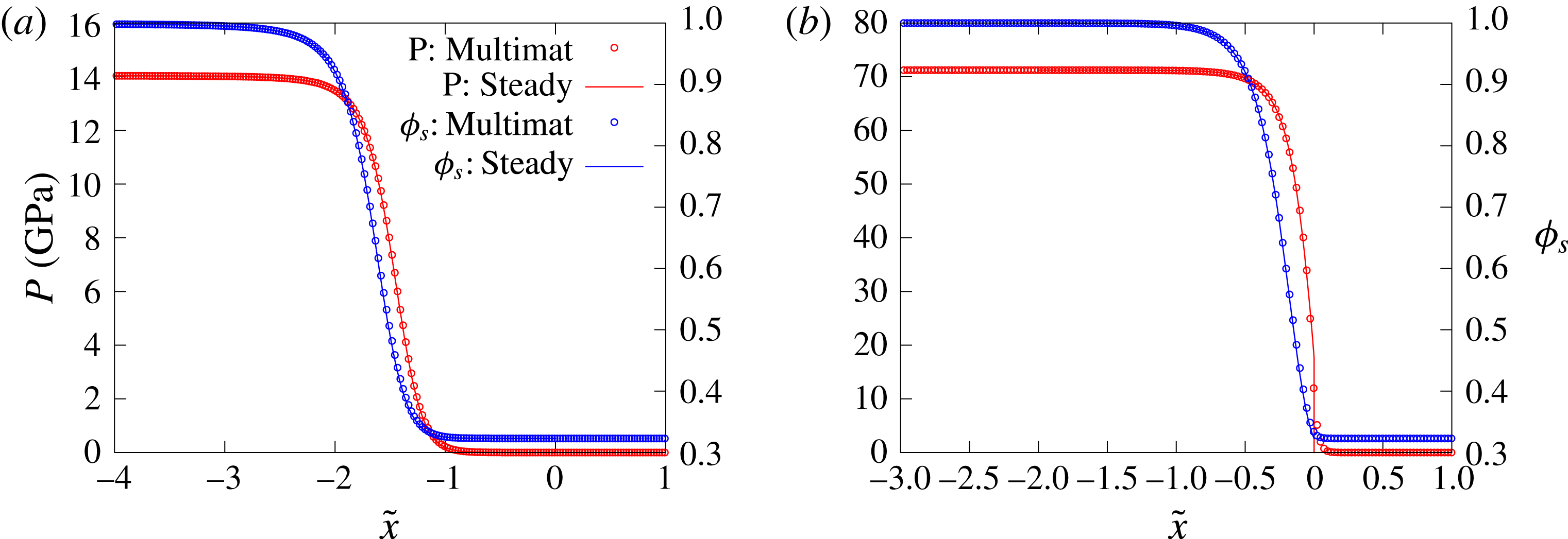
The ability of the MultiMat computational framework to accurately propagate detonations for various HE models including the Tait EOS based model described in § 2.1 has been demonstrated previously (e.g. Chiquete, Short, Meyer & Quirk (Reference Chiquete, Short, Meyer and Quirk2017)). We have also conducted a number of verification studies for the MultiMat implementation of the porous material compaction model described in § 2.2. Figure 10 shows a comparison of a MultiMat computation of a 1-D reverse impact problem for
 $\text{Npts}=20$
with the pressure
 $p$
and solid volume fraction
 $\unicode[STIX]{x1D719}_{s}$
derived from the steady travelling compaction wave solutions presented in § 3. Two cases are considered, one for fully dispersed subsonic flow and the other for supersonic shock-led flow. The 1-D MultiMat computations were initiated with spatially uniform uncompacted material travelling at
 $-u_{eq}$
toward a rigid wall on the left-hand side of the computational domain, where
 $u_{eq}$
is the flow speed of the compacted equilibrium state consistent with a target compaction wave speed
 $D_{0}$
(§ 3). A compaction wave develops, travelling to the right, with the solid volume fraction evolution equation (2.11) modifying the wave structure in time until a steady propagating wave is obtained. When shifted to a frame travelling at
 $-u_{eq}$
, this steady profile and wave speed
 $D_{0}$
can be compared with the 1-D steady travelling wave solution (§ 3) as shown in figure 10. For
 $\text{Npts}=20$
, the agreement between the MultiMat and steady travelling wave solutions is very good. For the supersonic case and for
 $\text{Npts}=20$
, the lead shock is slightly diffused, as expected for a shock capturing scheme. This improves for increased resolution.
Comparison of the pressure
 $p$
and solid volume fraction
 $\unicode[STIX]{x1D719}_{s}$
steady travelling compaction wave solutions derived in § 3 with a MultiMat computation for
 $\text{Npts}=20$
. Case (a) corresponds to a subsonic dispersed travelling wave solution with
 $D_{0}=3~\text{mm}~\unicode[STIX]{x03BC}\text{s}^{-1}$
,
 $\unicode[STIX]{x1D719}_{s0}=0.3229$
and
 $\bar{\unicode[STIX]{x1D707}}_{c}=2~\text{mm}^{-1}~\unicode[STIX]{x03BC}\text{s}~\text{GPa}$
(where
 $u_{eq}=2.0084~\text{mm}~\unicode[STIX]{x03BC}\text{s}^{-1}$
), while case (b) corresponds to a supersonic travelling wave solution with
 $D_{0}=7~\text{mm}~\unicode[STIX]{x03BC}\text{s}^{-1}$
,
 $\unicode[STIX]{x1D719}_{s0}=0.3229$
and
 $\bar{\unicode[STIX]{x1D707}}_{c}=4~\text{mm}^{-1}~\unicode[STIX]{x03BC}\text{s}~\text{GPa}$
(where
 $u_{eq}=4.3672~\text{mm}~\unicode[STIX]{x03BC}\text{s}^{-1}$
) that is led by a shock at the compaction wave front. For case (a), the MultiMat computation gives a wave speed
 $D_{0}=2.99989~\text{mm}~\unicode[STIX]{x03BC}\text{s}^{-1}$
, while for case (b)
 $D_{0}=6.99996~\text{mm}~\unicode[STIX]{x03BC}\text{s}^{-1}$
.
5.3 Results
5.3.1 High-speed HE1 detonation model
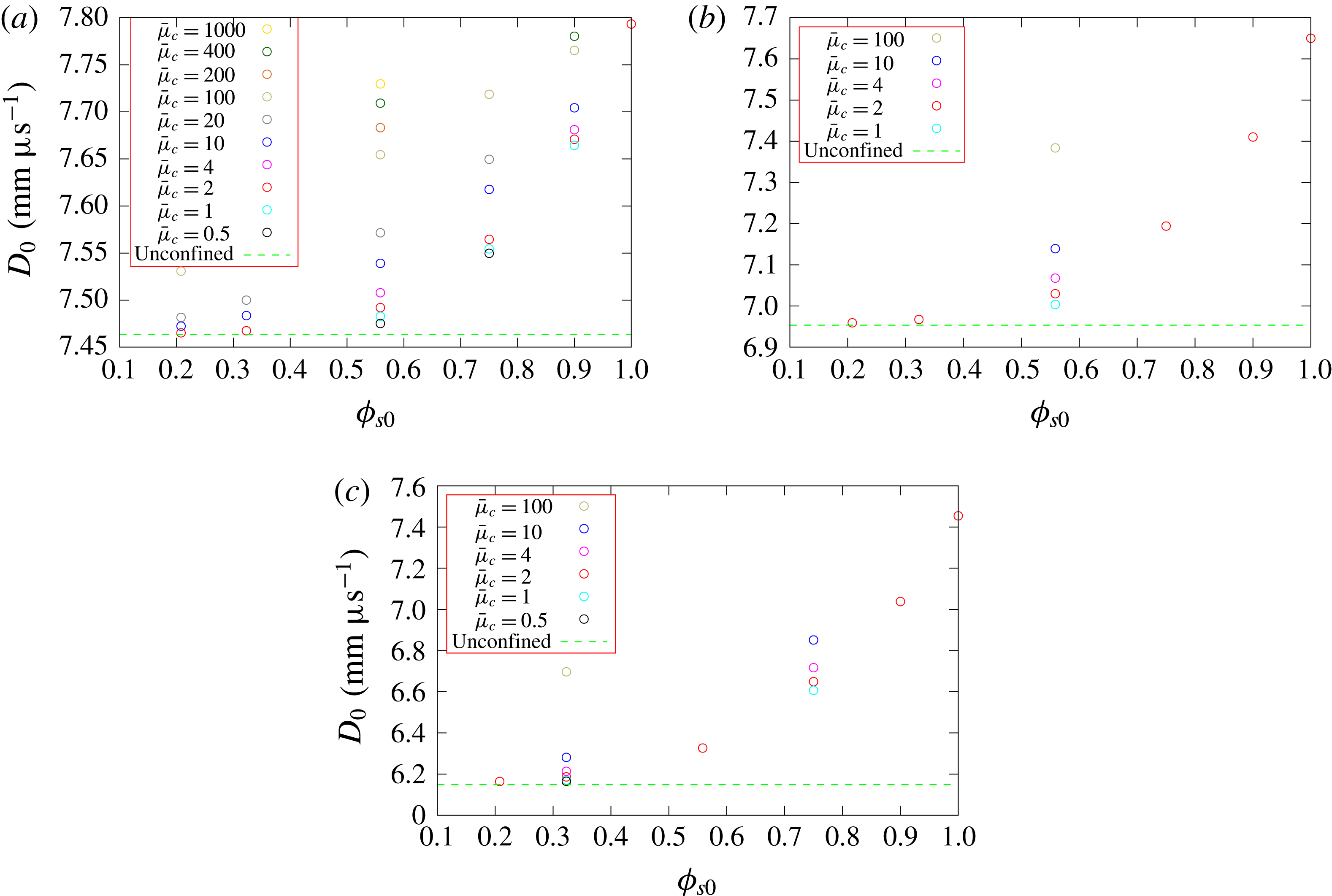
Figure 11 shows the dependence of the steady detonation phase speed,
 $D_{0}$
, for HE model HE1 for a range of porous confiner initial solid volume fractions
 $(\unicode[STIX]{x1D719}_{s0})$
and compaction viscosity magnitudes
 $(\bar{\unicode[STIX]{x1D707}}_{c})$
, as well as HE slab widths
 $(W_{HE})$
. Also shown is the detonation phase speed obtained for the selected HE slab widths when the confiner consists of a solid, but low-impedance material. We have chosen a low-impedance material representative of the elastomer Sylgard for this purpose, modelled by a
 $U_{s}-u_{p}$
equation of state (2.16) with
 $$\begin{eqnarray}\unicode[STIX]{x1D70C}_{s0}=0.84~\text{g}~\text{cc}^{-1},\quad c=1.127~\text{mm}~\unicode[STIX]{x03BC}\text{s}^{-1},\quad s=1.2,\quad \unicode[STIX]{x1D6E4}_{0}=1.5.\end{eqnarray}$$
This low-impedance material does not provide any confinement for a detonation modelled by HE1, and thus the detonation phase speed calculated with this confiner should represent the slowest possible for a given HE slab width. Figure 11a shows the
 $D_{0}$
variation for
 $W_{HE}=70$
. For a fixed compaction viscosity
 $\bar{\unicode[STIX]{x1D707}}$
, e.g.
 $\bar{\unicode[STIX]{x1D707}}=2~\text{mm}^{-1}~\unicode[STIX]{x03BC}\text{s}~\text{GPa}$
, we see that the phase speed increases significantly with increases in the initial solid volume fraction. Moreover, for
 $\bar{\unicode[STIX]{x1D707}}=2~\text{mm}^{-1}~\unicode[STIX]{x03BC}\text{s}~\text{GPa}$
, above the small initial solid volume fraction
 $\unicode[STIX]{x1D719}_{s0}=0.2097$
all values of
 $\unicode[STIX]{x1D719}_{s0}$
have a confining effect on detonation propagation. Only for the very low initial solid volume fraction
 $\unicode[STIX]{x1D719}_{s0}=0.2097$
has the detonation phase speed reached the unconfined (Sylgard) limit. This is consistent with the predictions of the oblique polar analysis (§ 4) that indicate even highly porous materials (moderately small
 $\unicode[STIX]{x1D719}_{s0}$
) could provide a strong confinement effect on detonation propagation.
Of particular interest though is the significant effect that the magnitude of the compaction viscosity
 $\bar{\unicode[STIX]{x1D707}}_{c}$
has on
 $D_{0}$
. For fixed
 $\unicode[STIX]{x1D719}_{s0}$
, increases in
 $\bar{\unicode[STIX]{x1D707}}_{c}$
, which increase the relaxation time for the compaction process and thus spread the compaction process out spatially, result in increasingly faster detonation phase speeds. Likewise, decreases in
 $\bar{\unicode[STIX]{x1D707}}_{c}$
, which spatially compress the compaction process, result in slower detonation phase speeds. The variation of
 $D_{0}$
with changes in the magnitude of
 $\bar{\unicode[STIX]{x1D707}}_{c}$
is significant. For instance, for
 $W_{HE}=70$
at
 $\unicode[STIX]{x1D719}_{s0}=0.5586$
,
 $D_{0}$
is
 $0.255~\text{mm}~\unicode[STIX]{x03BC}\text{s}^{-1}$
(or
 $255~\text{m}~\text{s}^{-1}$
) larger for
 $\bar{\unicode[STIX]{x1D707}}_{c}=1000~\text{mm}^{-1}~\unicode[STIX]{x03BC}\text{s}~\text{GPa}$
than for
 $\bar{\unicode[STIX]{x1D707}}_{c}=2~\text{mm}^{-1}~\unicode[STIX]{x03BC}\text{s}~\text{GPa}$
. Thus by increasing the relaxation time for the compaction process, the porous material confinement becomes effectively stronger, in the sense that the detonation phase speed is increased. Having a very rapid compaction process relative to the detonation reaction-zone time scale results in the weakest confinement effect (slowest
 $D_{0}$
). An additional observation is that the rate of change of
 $D_{0}$
with
 $\bar{\unicode[STIX]{x1D707}}_{c}$
first increases as
 $\bar{\unicode[STIX]{x1D707}}_{c}$
increases from the smaller
 $\bar{\unicode[STIX]{x1D707}}_{c}$
values calculated, before slowing for the largest values of
 $\bar{\unicode[STIX]{x1D707}}_{c}$
calculated. This indicates that the effect of increasing the detonation phase speed by continually spreading the compaction process will eventually saturate. Qualitatively similar behaviour to the above is seen in figure 11(b,c) for
 $W_{HE}=40$
and
 $W_{HE}=20$
. For these slab widths, even the smallest solid volume fraction
 $\unicode[STIX]{x1D719}_{s0}=0.2097$
calculated appears to be slightly confining. The dynamics underlying the variation in
 $D_{0}$
with
 $\unicode[STIX]{x1D719}_{s0}$
and
 $\bar{\unicode[STIX]{x1D707}}_{c}$
is now explored.
Variation of the detonation phase speed
 $D_{0}$
with confiner initial solid volume fraction
 $(\unicode[STIX]{x1D719}_{s0})$
and compaction viscosity magnitude
 $(\bar{\unicode[STIX]{x1D707}}_{c})$
for three HE slab widths: (a)
 $W_{HE}=70$
, (b)
 $W_{HE}=40$
and (c)
 $W_{HE}=20$
. The HE model is HE1. The units of the scaled compaction viscosity
 $\bar{\unicode[STIX]{x1D707}}_{c}$
are
 $\text{mm}^{-1}~\unicode[STIX]{x03BC}\text{s}~\text{GPa}$
. For any given
 $\unicode[STIX]{x1D719}_{s0}$
, the circles show the specific
 $\bar{\unicode[STIX]{x1D707}}_{c}$
cases that were calculated. Note all cases are distinct, and so fewer circles at a given
 $\unicode[STIX]{x1D719}_{s0}$
indicates fewer simulations were run, rather than overlapping results.
The variations in detonation phase speed
 $D_{0}$
are related to the way in which the porous confiner compaction process is influenced by pressure loading from the HE detonation and vice versa. Figure 12 shows pressure gradient images of the flow variation in the HE and porous confiner in the vicinity of the detonation front for
 $\bar{\unicode[STIX]{x1D707}}_{c}=2~\text{mm}^{-1}~\unicode[STIX]{x03BC}\text{s}~\text{GPa}$
,
 $W_{HE}=70$
and
 $\unicode[STIX]{x1D719}_{s0}=0.2079$
,
 $0.5586$
and
 $0.9$
. Also shown is the corresponding structure for the solid material with
 $\unicode[STIX]{x1D719}_{s0}=1$
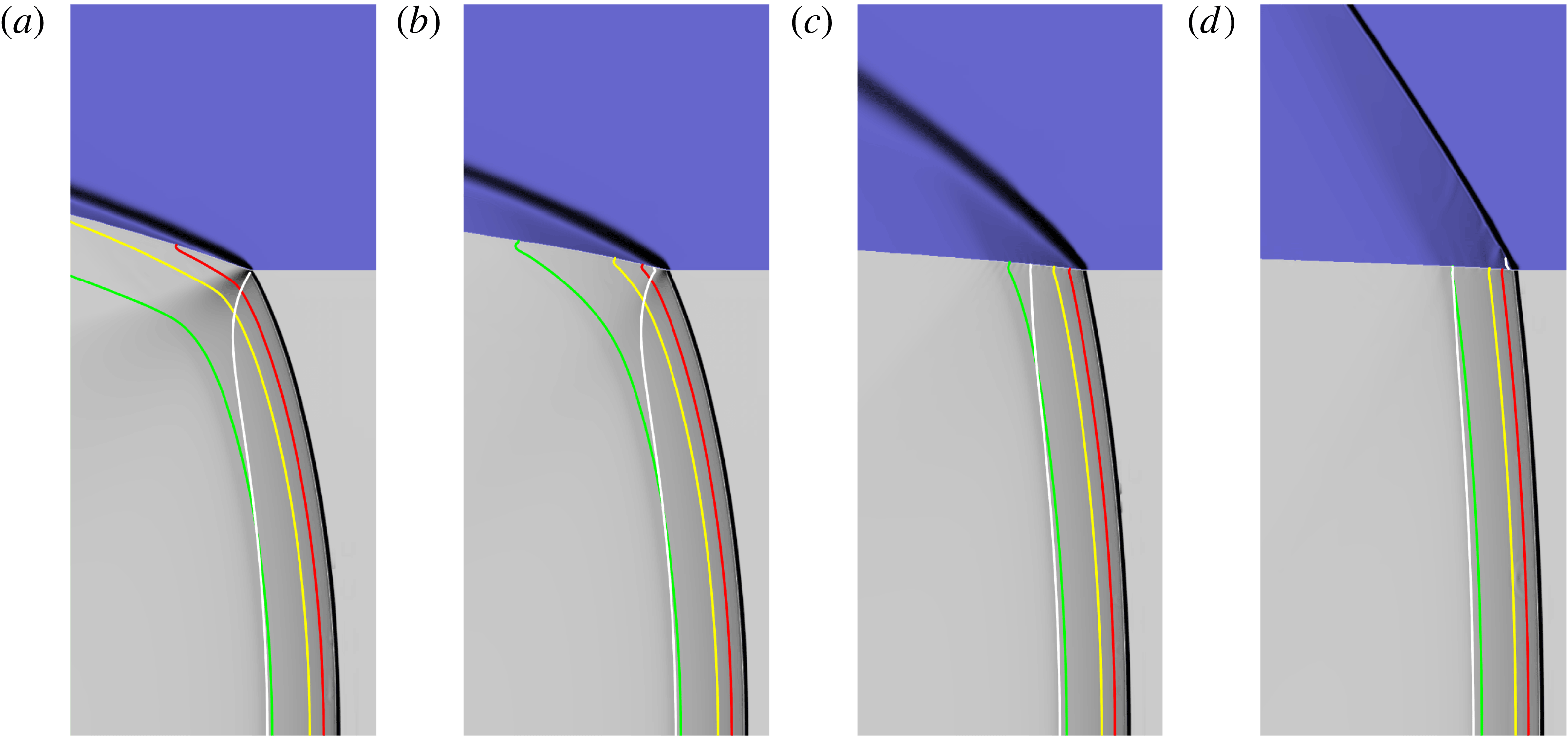
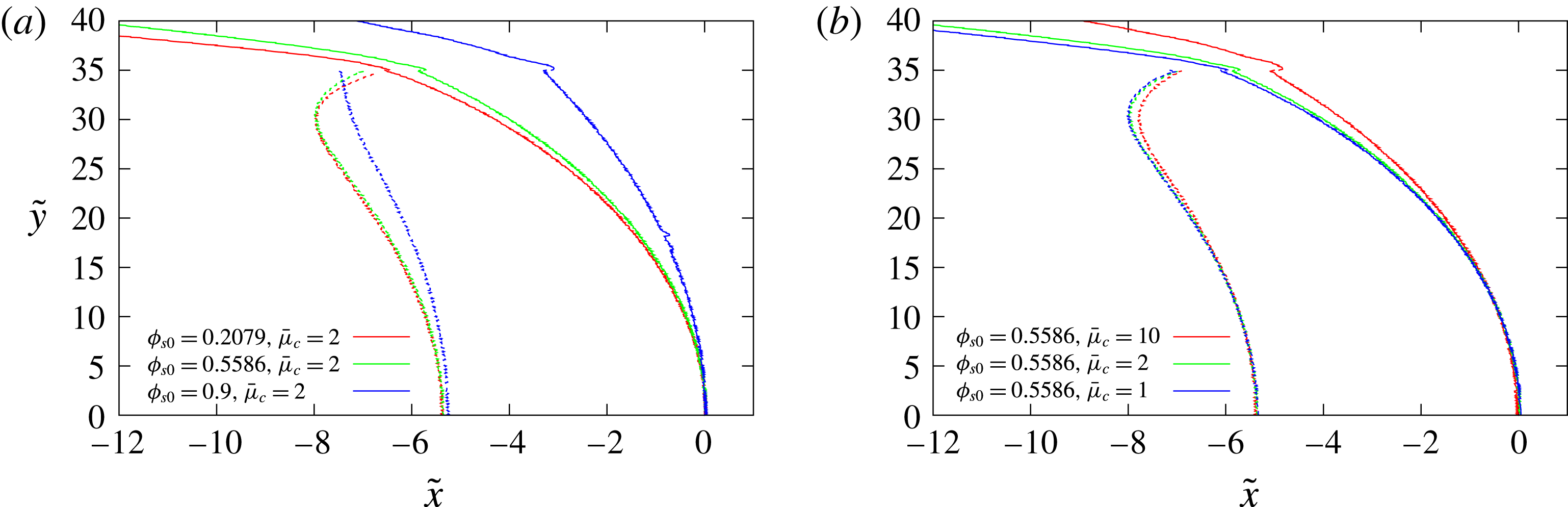
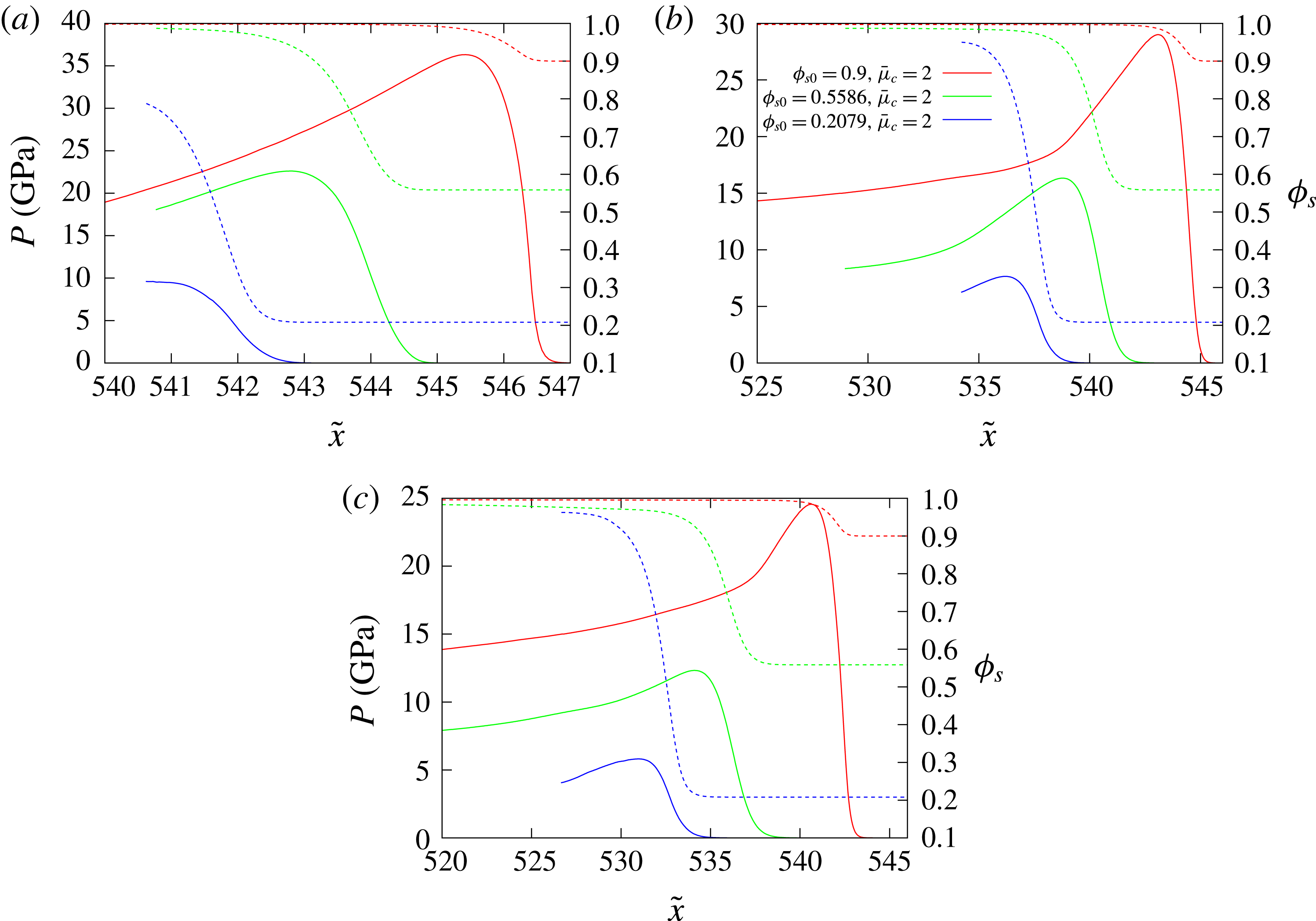
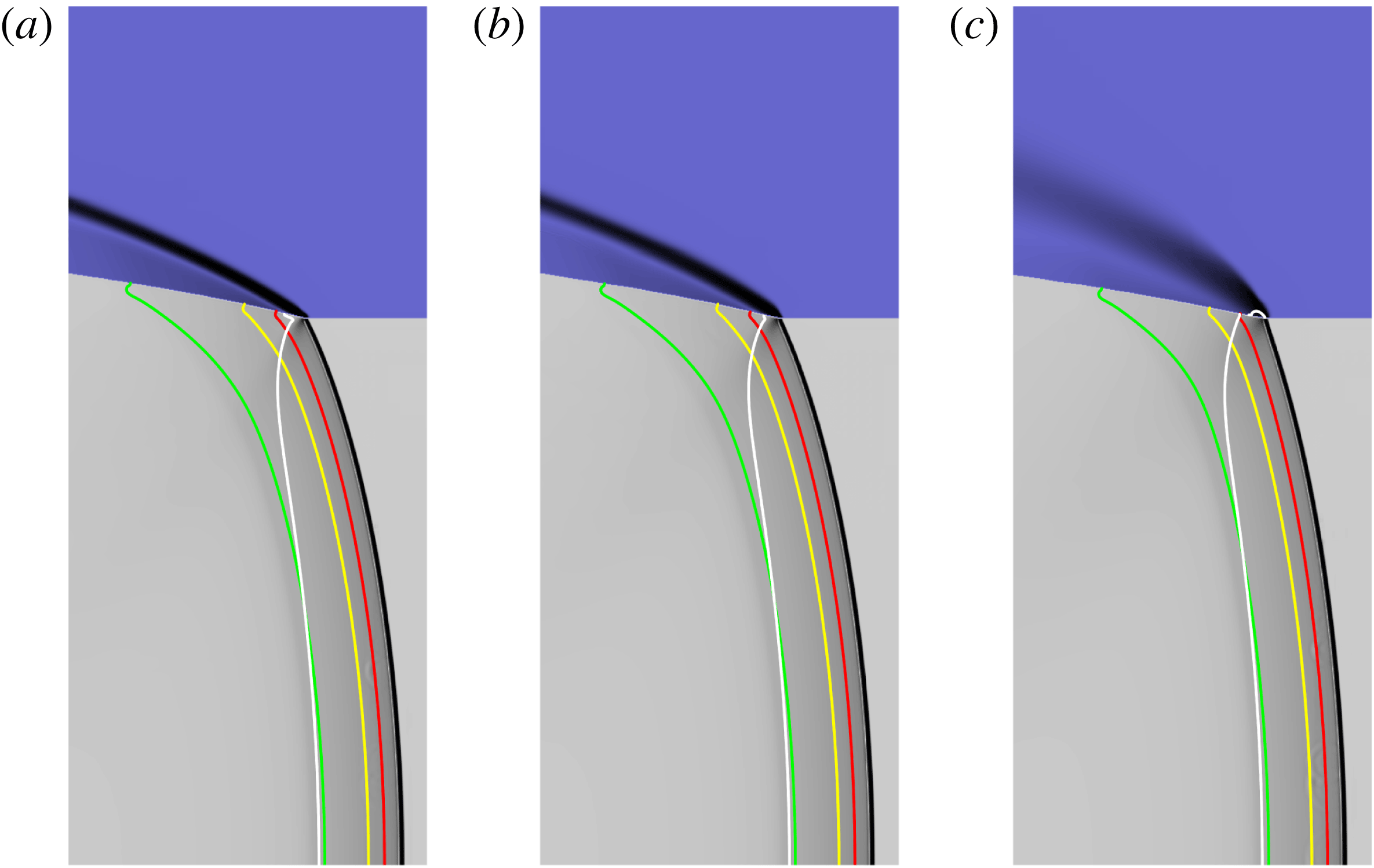
. The pressure gradient images are designed to shade the regions of strongest variation in pressure gradient for each of the two materials. The specific methodology for generating the pressure gradient images from the computational flow solution is presented in appendix A. These images do not contain quantitative data, but are insightful as they play a role similar to the effect of Schlieren imaging of compressible flows, highlighting the position of prominent wave structures. Also added to the pressure gradient images are contours in the HE and confiner representing the sonic flow locus in a frame travelling with the steady detonation shock, and in the HE various reactant depletion contours showing the progress of reaction. Figure 13 shows a comparison of the location of the detonation shock, confiner compaction wavehead and the detonation sonic locus across the HE–confiner slab for the three porous confiner cases shown in figure 12. The detonation shock location is given by the points where
 $p=1~\text{GPa}$
, the compaction wavehead by
 $p=1~\text{GPa}$
and the sonic line by the locus in which the flow Mach number is one. Figure 14 contains spatial profiles of the
 $p$
and
 $\unicode[STIX]{x1D719}_{s}$
variation in the porous confiner along the axial lines
 ${\tilde{y}}=36$
,
 ${\tilde{y}}=38$
and
 ${\tilde{y}}=40$
for the three porous cases shown in figure 12. We have also repeated the oblique wave polar analysis in § 4 for the specific phase speeds
 $D_{0}$
calculated in figure 12. The combination of this information can be used to build up an understanding of the influence of the porous confiner for variable
 $\unicode[STIX]{x1D719}_{s0}$
.
Pressure gradient images highlighting regions of strongest variation in the pressure gradient for each material in the vicinity of the detonation front for different
 $\unicode[STIX]{x1D719}_{s0}$
with
 $\bar{\unicode[STIX]{x1D707}}_{c}=2~\text{mm}^{-1}~\unicode[STIX]{x03BC}\text{s}~\text{GPa}$
. The HE model is HE1. The HE slab width is
 $W_{HE}=70$
. (a)
 $\unicode[STIX]{x1D719}_{s0}=0.2079$
. The calculated detonation phase speed is
 $D_{0}=7.465~\text{mm}~\unicode[STIX]{x03BC}\text{s}^{-1}$
. (b)
 $\unicode[STIX]{x1D719}_{s0}=0.5586$
. Speed is
 $D_{0}=7.492~\text{mm}~\unicode[STIX]{x03BC}\text{s}^{-1}$
. (c)
 $\unicode[STIX]{x1D719}_{s0}=0.9$
. Speed is
 $D_{0}=7.671~\text{mm}~\unicode[STIX]{x03BC}\text{s}^{-1}$
. (d) The wave structure when the confiner is solid,
 $\unicode[STIX]{x1D719}_{s0}=1$
. Speed is
 $D_{0}=7.793~\text{mm}~\unicode[STIX]{x03BC}\text{s}^{-1}$
. Each image has a width of
 $\tilde{x}=23$
and a height of
 ${\tilde{y}}=55$
, where the bottom boundary is the channel symmetry line
 $({\tilde{y}}=0)$
. The white line is the sonic flow contour in the HE and confiner regions in a frame travelling with the steady detonation front. The red, yellow and green lines represent 50, 75 and 99 % HE reactant depletion contours respectively.
Comparison of the location of the detonation shock and confiner compaction wavehead (solid lines) and the detonation sonic locus (dashed lines) across the HE–confiner slab for the porous confiner cases shown in (a) figure 12 and (b) figure 15. The symmetry axis is along
 ${\tilde{y}}=0$
. For each case, the reference point has been set such that the detonation shock location along the symmetry line
 ${\tilde{y}}=0$
has been shifted to
 $\tilde{x}=0$
.
Spatial profiles of the
 $p$
(solid lines) and
 $\unicode[STIX]{x1D719}_{s}$
(dashed lines) variation in the porous confiner along the axial lines (a)
 ${\tilde{y}}=36$
, (b)
 ${\tilde{y}}=38$
and (c)
 ${\tilde{y}}=40$
for the three porous confiner cases shown in figure 12.
One prominent feature of figure 12 is the rapid increase in obliqueness of the compaction wave in the confiner as the initial solid volume fraction is decreased. This property is consistent with the polar analysis in § 4, which showed the rapid increase in maximum streamline turning angle as the initial material porosity was increased. For the lowest initial solid volume fraction (figure 12
a),
 $\unicode[STIX]{x1D719}_{s0}=0.2079$
, the sonic line in the HE intersects the confiner interface close to the detonation shock. This is a case of weak confinement, where the detonation driving zone is isolated from the material properties and flow in the confiner. A PM fan is observed in the HE that originates from the intersection of the detonation shock with the confiner interface. The flow in the confiner is supersonic, consistent with the polar analysis. Reaction at the edge of the charge slows significantly (figure 12
a). Only moderate pressure is built up in the confiner (figure 14) which decays rapidly with confiner depth. For
 $\unicode[STIX]{x1D719}_{s0}=0.5586$
(figure 12
b), the sonic locus now intersects the confiner interface behind the detonation shock, and thus there is a region of subsonic flow in the HE at the confiner interface. This corresponds to strong confinement, where the detonation driving zone structure is directly influenced by the presence of the confiner. The detonation shock is flatter than that observed for
 $\unicode[STIX]{x1D719}_{s0}=0.2079$
(figure 13
a). Interestingly, as is apparent from figures 12 and 13(a), the compaction wavehead appears to lie slightly ahead of the detonation shock at the confiner interface. This feature implies that the compaction wavehead is driving the detonation shock at the material interface, which is the structure of the local wave pattern predicted by the compaction shock–detonation shock polar analysis described in figure 8. Such an interaction is possible when the compaction relaxation time is finite. The presence and reproducibility of this feature has been confirmed with equivalent simulations run at higher resolutions. The pressures generated in the confiner by the detonation loading and compaction process are higher than those for
 $\unicode[STIX]{x1D719}_{s0}=0.2079$
, while the compaction region near the interface spatially extends across some distance of the detonation driving zone (figures 13
a and 14). For
 $\unicode[STIX]{x1D719}_{s0}=0.9$
, there is a significant subsonic region in the HE at the confiner interface, while the flow in the confiner is again entirely supersonic. In contrast, the polar analysis conducted for
 $D_{0}=7.671~\text{mm}~\unicode[STIX]{x03BC}\text{s}^{-1}$
and
 $\unicode[STIX]{x1D719}_{s0}=0.9$
has the direct intersection point of the detonation shock and compaction wave polars (assuming instantaneous compaction) on the subsonic branch of the compaction polar. The compaction wavehead again runs slightly ahead of the detonation shock at the confiner interface (figure 13
a). High pressures are generated in the confiner, and thus the compaction region is comparatively short. For the compaction region depths considered in figure 14, only the low porosity initial state
 $\unicode[STIX]{x1D719}_{s0}=0.9$
attains a state of nearly fully compacted material behind the oblique compaction wave. For higher initial porosities, the material confining the detonation in the region of the material interface is not fully compacted.
The observations made above of the increases in
 $D_{0}$
due to increasing
 $\unicode[STIX]{x1D719}_{s0}$
are in part due to the higher density of the starting material, in addition to the mechanisms of the compaction process. For fixed
 $\unicode[STIX]{x1D719}_{s0}$
and variable
 $\bar{\unicode[STIX]{x1D707}}_{c}$
this is not the case, and the dynamics of how significant increases in
 $D_{0}$
can occur for increasing
 $\bar{\unicode[STIX]{x1D707}}_{c}$
, as seen in figure 12, is now explored. Figure 15 shows pressure gradient images of the flow structures in the HE and porous confiner in the vicinity of the detonation front for
 $\unicode[STIX]{x1D719}_{s0}=0.5586$
and
 $W_{HE}=70$
, and for
 $\bar{\unicode[STIX]{x1D707}}_{c}=1$
(where
 $D_{0}=7.483~\text{mm}~\unicode[STIX]{x03BC}\text{s}^{-1}$
)
 $\bar{\unicode[STIX]{x1D707}}_{c}=2$
(where
 $D_{0}=7.492~\text{mm}~\unicode[STIX]{x03BC}\text{s}^{-1}$
) and
 $\bar{\unicode[STIX]{x1D707}}_{c}=10~\text{mm}^{-1}~\unicode[STIX]{x03BC}\text{s}~\text{GPa}$
(where
 $D_{0}=7.539~\text{mm}~\unicode[STIX]{x03BC}\text{s}^{-1}$
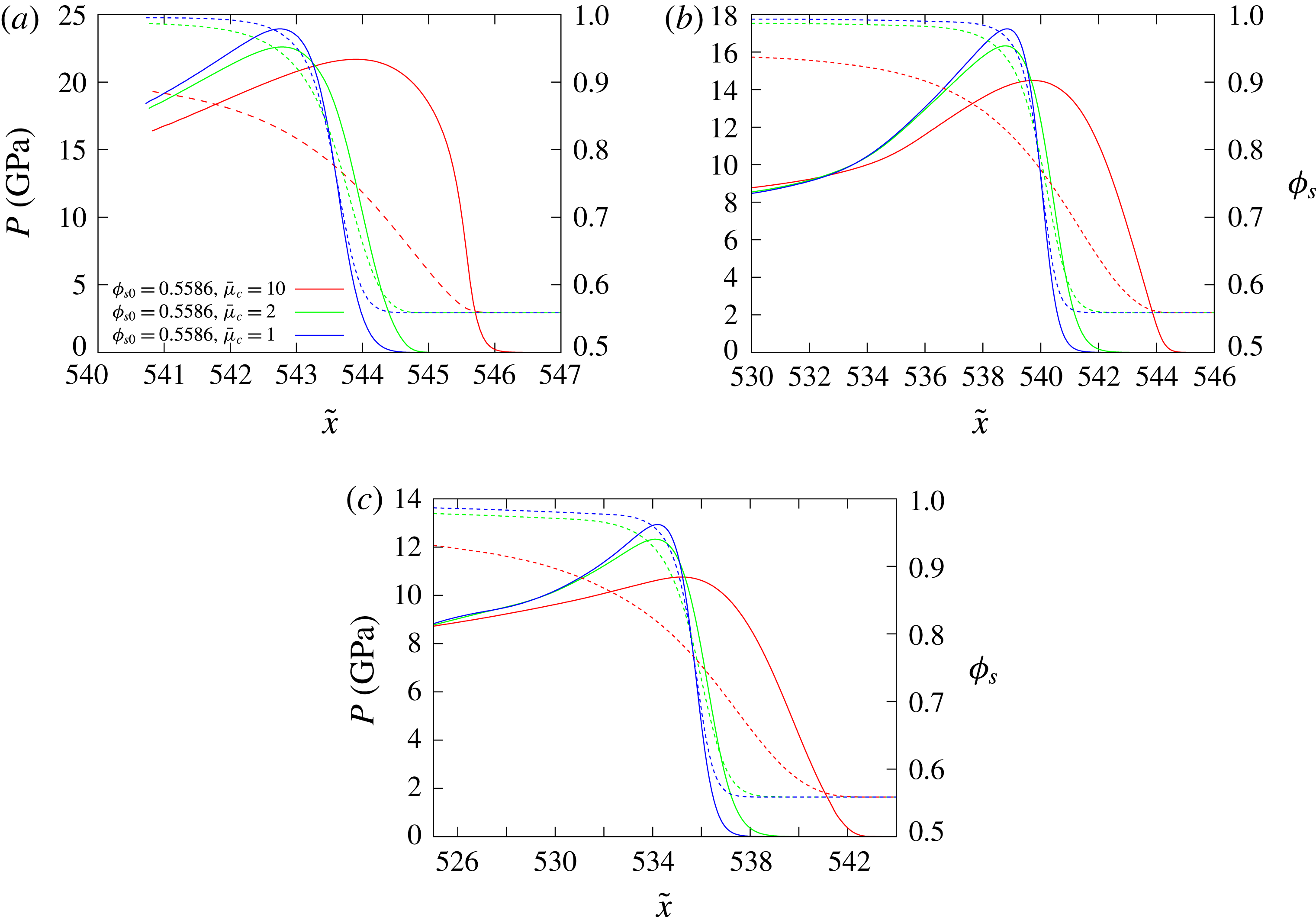
). Figure 13(b) shows a comparison of the location of the detonation shock, confiner compaction wavehead and the detonation sonic locus across the HE–confiner slab for the three cases shown figure 15. Figure 16 contains spatial profiles of the
 $p$
and
 $\unicode[STIX]{x1D719}_{s}$
variation in the porous confiner along the axial lines
 ${\tilde{y}}=36$
,
 ${\tilde{y}}=38$
and
 ${\tilde{y}}=40$
for the three cases shown in figure 15. In all the simulations we have conducted, increasing
 $\bar{\unicode[STIX]{x1D707}}_{c}$
at fixed
 $\unicode[STIX]{x1D719}_{s0}$
causes
 $D_{0}$
to increase. Thus slowing the compaction rate for a given HE pressure loading leads to a stronger confinement effect on detonation propagation.
As for figure 12, but with
 $\unicode[STIX]{x1D719}_{s0}=0.5586$
and (a)
 $\bar{\unicode[STIX]{x1D707}}_{c}=1~\text{mm}^{-1}~\unicode[STIX]{x03BC}\text{s}~\text{GPa}$
with a calculated detonation phase speed of
 $D_{0}=7.483~\text{mm}~\unicode[STIX]{x03BC}\text{s}^{-1}$
, (b)
 $\bar{\unicode[STIX]{x1D707}}_{c}=2~\text{mm}^{-1}~\unicode[STIX]{x03BC}\text{s}~\text{GPa}$
with detonation speed
 $D_{0}=7.492~\text{mm}~\unicode[STIX]{x03BC}\text{s}^{-1}$
, (c)
 $\bar{\unicode[STIX]{x1D707}}_{c}=10~\text{mm}^{-1}~\unicode[STIX]{x03BC}\text{s}~\text{GPa}$
with detonation speed
 $D_{0}=7.539~\text{mm}~\unicode[STIX]{x03BC}\text{s}^{-1}$
. Each image has a width of
 $\tilde{x}=23$
and a height of
 ${\tilde{y}}=55$
, where the bottom boundary is the channel symmetry line
 $({\tilde{y}}=0)$
.
Spatial profiles of the
 $p$
(solid lines) and
 $\unicode[STIX]{x1D719}_{s}$
(dashed lines) variation in the porous confiner along the axial lines (a)
 ${\tilde{y}}=36$
, (b)
 ${\tilde{y}}=38$
and (c)
 ${\tilde{y}}=40$
for the three cases shown in figure 15.
Several issues are at work. From figures 15 and 16, it is apparent that as
 $\bar{\unicode[STIX]{x1D707}}_{c}$
increases, the thickness of the dominant pressure gradient regions in the confiner increase. Further, the dominant pressure gradient region becomes more focused in the confiner region near the HE interface (figure 15
c). As
 $\bar{\unicode[STIX]{x1D707}}_{c}$
increases, the extent of the subsonic region in the HE at the confiner interface increases as the sonic line drops further back from the detonation shock, while the detonation shock becomes flatter. These properties are characteristic of those traditionally seen for increasingly stronger detonation confinement by increasingly denser solid material confiners. In the three cases shown in figure 15, the flow in the confiner is everywhere supersonic, except for
 $\bar{\unicode[STIX]{x1D707}}_{c}=10~\text{mm}^{-1}~\unicode[STIX]{x03BC}\text{s}~\text{GPa}$
where a small subsonic region is present near the material interface. The oblique polar theory, based on rapid compaction relaxation times, predicts the flow in the confiner will be supersonic in all three cases at the detonation shock–compaction wave polar direct match point. The compaction wavehead lies ahead of the detonation shock in all three cases, becoming prominent for
 $\bar{\unicode[STIX]{x1D707}}_{c}=10~\text{mm}^{-1}~\unicode[STIX]{x03BC}\text{s}~\text{GPa}$
, and implying that the compaction wavehead is locally driving the detonation shock (figure 8). The pressure and solid volume fraction evolution in the compaction zone of the confiner are instructive (figure 16). The peak pressure reached in the compaction zone at each depth is actually higher for the smallest compaction viscosity
 $\bar{\unicode[STIX]{x1D707}}_{c}=1~\text{mm}^{-1}~\unicode[STIX]{x03BC}\text{s}~\text{GPa}$
, and lowest for the largest compaction viscosity
 $\bar{\unicode[STIX]{x1D707}}_{c}=10~\text{mm}^{-1}~\unicode[STIX]{x03BC}\text{s}~\text{GPa}$
. Also, increasingly higher degrees of compaction are attained as
 $\bar{\unicode[STIX]{x1D707}}_{c}$
is lowered. However, the width of the compaction zone across which high pressures in the compaction zone are sustained is significantly larger for the largest compaction viscosity
 $\bar{\unicode[STIX]{x1D707}}_{c}=10~\text{mm}^{-1}~\unicode[STIX]{x03BC}\text{s}~\text{GPa}$
. The width of the compaction region for
 $\bar{\unicode[STIX]{x1D707}}_{c}=2~\text{mm}^{-1}~\unicode[STIX]{x03BC}\text{s}~\text{GPa}$
is slightly larger than for
 $\bar{\unicode[STIX]{x1D707}}_{c}=1~\text{mm}^{-1}~\unicode[STIX]{x03BC}\text{s}~\text{GPa}$
at comparable depths. The conclusion that one draws is that slowing the rate of compaction results in an increasingly stronger confinement effect on the detonation as the longer relaxation time for compaction sustains higher pressures across the width of the detonation reaction zone at the confiner interface and beyond. The pressure release that occurs in the porous confiner after the compaction zone for the lower compaction viscosities, where thinner compaction zones are generated relative to the detonation reaction zone, results in a weaker confinement of the detonation even though higher pressures are generated in the thinner compaction zone.
5.3.2 Low-speed HE2 detonation model
We now turn to the study of HE model HE2, representative of the properties of a low-detonation-speed HE. For solid material confiners, having a detonation speed lower than the confiner sound speed leads to a complex flow interaction between the confiner and HE regions, where large amplitude pressure waves in the confiner can penetrate ahead of the detonation front (Sharpe & Bdzil Reference Sharpe and Bdzil2006; Short et al.
Reference Short, Quirk, Kiyanda, Jackson, Briggs and Shinas2010). Significant variations in detonation wave speed with confiner thickness have also been observed (Short et al.
Reference Short, Quirk, Kiyanda, Jackson, Briggs and Shinas2010). When the confiner is solid, steady propagating pressure wave solutions in the confiner are not possible when the wave speed is lower than the sound speed. With a porous material confiner, however, steady travelling, fully dispersed subsonic compaction waves are possible with
 $D_{0}<C_{s0}$
as shown in § 3. Here we explore issues of detonation confinement with HE model HE2 and the porous material confiner when
 $D_{0}<C_{s0}$
.
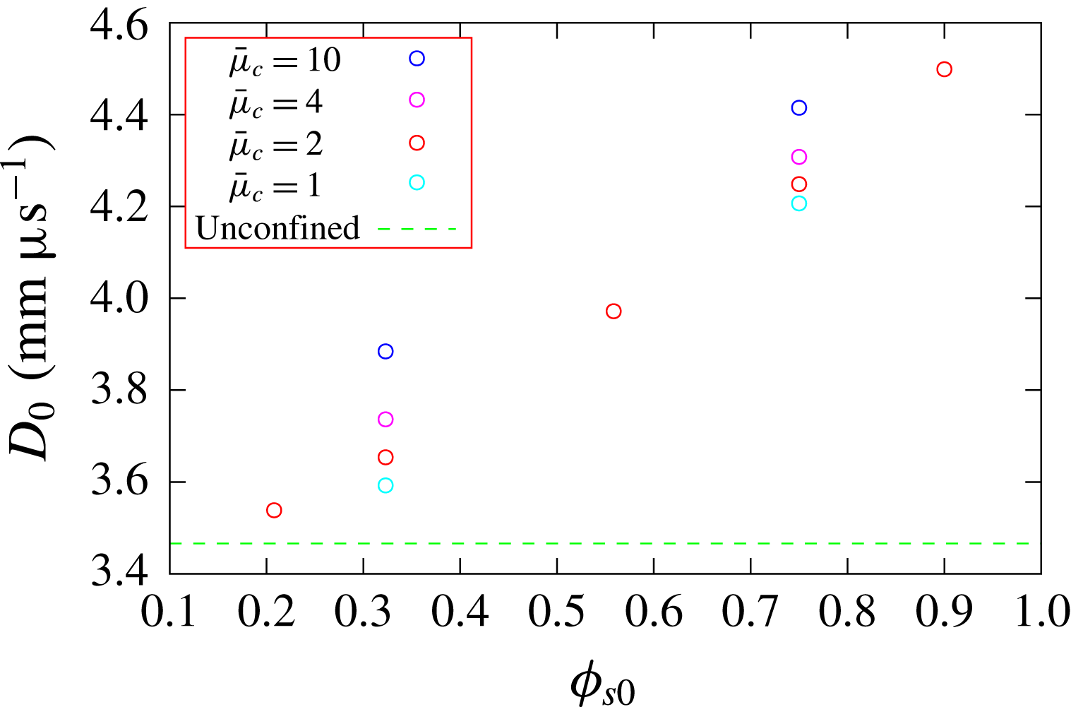
Figure 17 shows the dependence of the detonation phase speed for HE model HE2 with
 $W_{HE}=20$
for a range of confiner initial solid volume fractions
 $(\unicode[STIX]{x1D719}_{s0})$
and compaction viscosity magnitudes
 $(\bar{\unicode[STIX]{x1D707}}_{c})$
. Similar trends exist to that described above for the HE1 model. All cases show strong confinement by the porous confiner, where the calculated detonation phase speeds
 $D_{0}$
are above the unconfined limit for
 $W_{HE}=20$
. For fixed
 $\bar{\unicode[STIX]{x1D707}}_{c}$
, increases in
 $\unicode[STIX]{x1D719}_{s0}$
result in higher detonation phase speeds. Similarly, at fixed
 $\unicode[STIX]{x1D719}_{s0}$
, increases in
 $\bar{\unicode[STIX]{x1D707}}_{c}$
also lead to higher detonation phase speeds, where again the effect on
 $D_{0}$
of increasing the compaction viscosity amplitude is quite significant.
Variation of the detonation phase speed
 $D_{0}$
with confiner initial solid volume fraction
 $(\unicode[STIX]{x1D719}_{s0})$
and compaction viscosity magnitude
 $(\bar{\unicode[STIX]{x1D707}}_{c})$
. The HE model is HE2 and
 $W_{HE}=20$
. The units of the scaled compaction viscosity
 $\bar{\unicode[STIX]{x1D707}}_{c}$
are
 $\text{mm}^{-1}~\unicode[STIX]{x03BC}\text{s}~\text{GPa}$
. As with figure 11, for a given
 $\unicode[STIX]{x1D719}_{s0}$
, the circles show the specific
 $\bar{\unicode[STIX]{x1D707}}_{c}$
cases that were run. All cases are distinct, and so fewer circles at a given
 $\unicode[STIX]{x1D719}_{s0}$
indicates fewer simulations were run, rather than overlapping results.
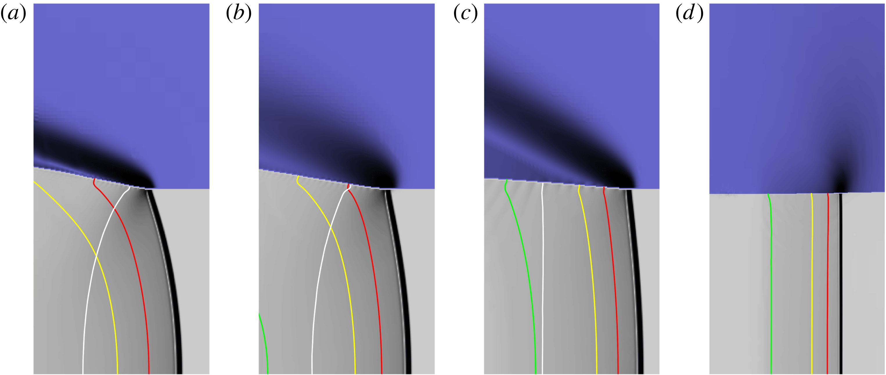
Pressure gradient images highlighting regions of strongest variation in the pressure gradient for each material in the vicinity of the detonation front for different
 $\unicode[STIX]{x1D719}_{s0}$
and
 $\bar{\unicode[STIX]{x1D707}}_{c}$
. The HE model is HE2. The HE slab width is
 $W_{HE}=20$
. (a)
 $\unicode[STIX]{x1D719}_{s0}=0.3229$
,
 $\bar{\unicode[STIX]{x1D707}}_{c}=2~\text{mm}^{-1}~\unicode[STIX]{x03BC}\text{s}~\text{GPa}$
. The calculated detonation phase speed is
 $D_{0}=3.654~\text{mm}~\unicode[STIX]{x03BC}\text{s}^{-1}$
. (b)
 $\unicode[STIX]{x1D719}_{s0}=0.3229$
,
 $\bar{\unicode[STIX]{x1D707}}_{c}=10~\text{mm}^{-1}~\unicode[STIX]{x03BC}\text{s}~\text{GPa}$
with
 $D_{0}=3.884~\text{mm}~\unicode[STIX]{x03BC}\text{s}^{-1}$
. (c)
 $\unicode[STIX]{x1D719}_{s0}=0.75$
,
 $\bar{\unicode[STIX]{x1D707}}_{c}=2~\text{mm}^{-1}~\unicode[STIX]{x03BC}\text{s}~\text{GPa}$
with
 $D_{0}=4.249~\text{mm}~\unicode[STIX]{x03BC}\text{s}^{-1}$
. (d) The wave structure when the confiner is solid,
 $\unicode[STIX]{x1D719}_{s0}=1$
, with detonation speed
 $D_{0}=4.940~\text{mm}~\unicode[STIX]{x03BC}\text{s}^{-1}$
. Each image has a width of
 $\tilde{x}=9.5$
and a height of
 ${\tilde{y}}=20$
, where the bottom boundary is the channel symmetry line
 $({\tilde{y}}=0)$
. Contour definitions as in figure 12.
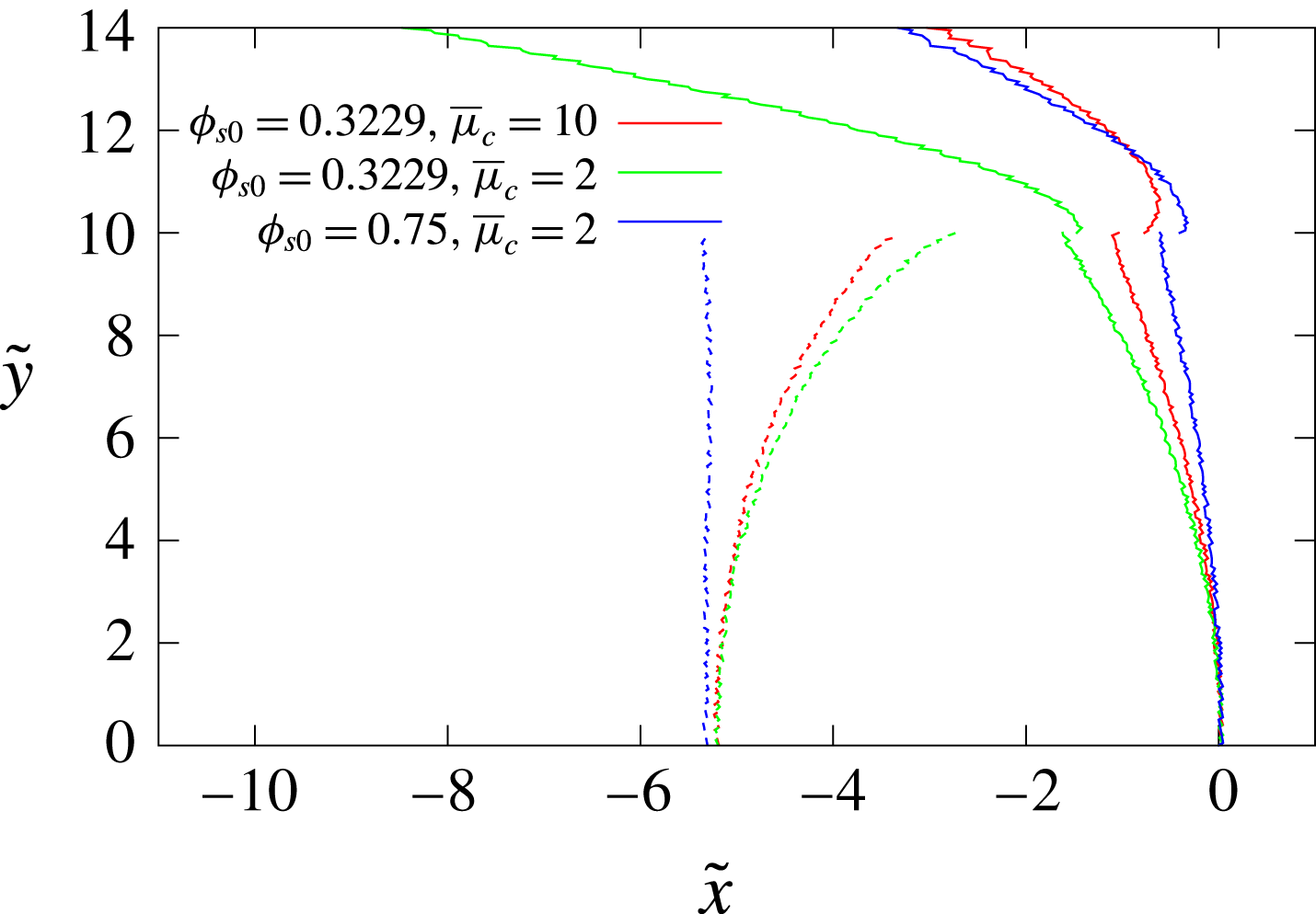
Comparison of the location of the detonation shock and confiner compaction wavehead (solid lines) and the detonation sonic locus (dashed lines) across the HE/confiner slab for the three porous confiner cases shown in figure 18. The symmetry axis is along
 ${\tilde{y}}=0$
. For each case, the reference point has been set such that the detonation shock location along
 ${\tilde{y}}=0$
has been shifted to
 $\tilde{x}=0$
.
Spatial profiles of the
 $p$
(solid lines) and
 $\unicode[STIX]{x1D719}_{s}$
(dashed lines) variation in the confiner for the three porous confiner cases shown in figure 18 along the axial lines (a)
 ${\tilde{y}}=11$
, (b)
 ${\tilde{y}}=13$
and (c)
 ${\tilde{y}}=15$
.
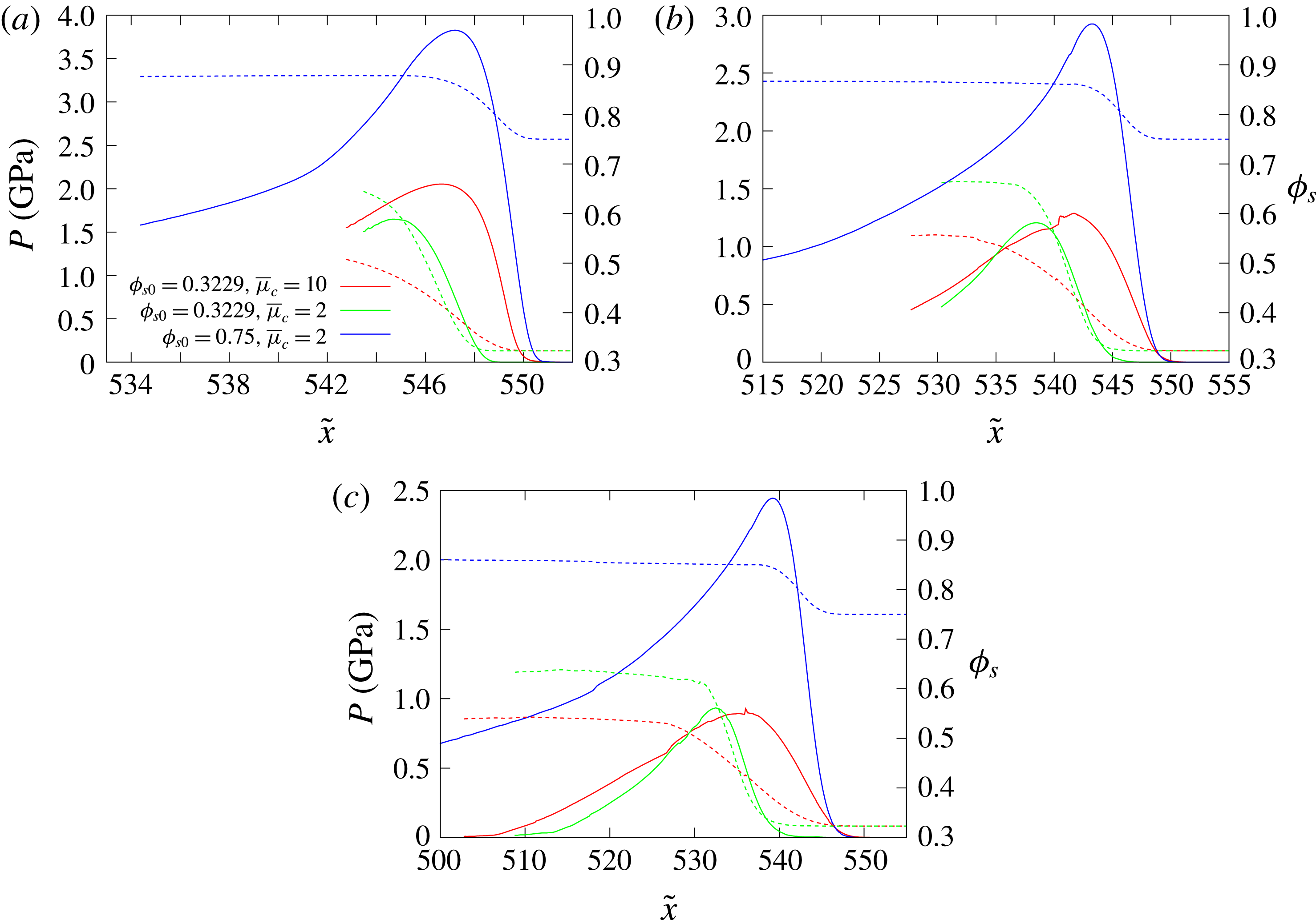
Figure 18 shows pressure gradient images of the flow in the HE and porous confiner in the vicinity of the detonation front for
 $W_{HE}=20$
,
 $\unicode[STIX]{x1D719}_{s0}=0.3229$
and
 $\bar{\unicode[STIX]{x1D707}}_{c}=2~\text{mm}^{-1}~\unicode[STIX]{x03BC}\text{s}~\text{GPa}$
(where
 $D_{0}=3.654~\text{mm}~\unicode[STIX]{x03BC}\text{s}^{-1}$
),
 $\unicode[STIX]{x1D719}_{s0}=0.3229$
and
 $\bar{\unicode[STIX]{x1D707}}_{c}=10~\text{mm}^{-1}~\unicode[STIX]{x03BC}\text{s}~\text{GPa}$
(where
 $D_{0}=3.884~\text{mm}~\unicode[STIX]{x03BC}\text{s}^{-1}$
) and
 $\unicode[STIX]{x1D719}_{s0}=0.75$
and
 $\bar{\unicode[STIX]{x1D707}}_{c}=2~\text{mm}^{-1}~\unicode[STIX]{x03BC}\text{s}~\text{GPa}$
(where
 $D_{0}=4.249~\text{mm}~\unicode[STIX]{x03BC}\text{s}^{-1}$
). Also shown is the pressure gradient image for solid confiner material
 $(\unicode[STIX]{x1D719}_{s0}=1)$
. Figure 19 shows a comparison of the location of the detonation shock, confiner compaction wavehead and the detonation sonic locus across the HE–confiner slab for the three porous confiner cases shown figure 18. Figure 20 contains spatial profiles of the
 $p$
and
 $\unicode[STIX]{x1D719}_{s}$
variation in the porous confiner along the axial lines
 ${\tilde{y}}=11$
,
 ${\tilde{y}}=13$
and
 ${\tilde{y}}=15$
for the three porous material cases shown in figure 18.
For the solid confiner case (figure 18
d), there is a region of high pressure in the confiner focused near the interface. The material interface is initially deflected into the HE, causing the detonation front to become concave, and driving the detonation phase speed above the CJ detonation speed. These are typical characteristics of detonation confinement by solid high-sound-speed confiners when
 $D_{0}<C_{s0}$
(Sharpe & Bdzil Reference Sharpe and Bdzil2006; Short et al.
Reference Short, Quirk, Kiyanda, Jackson, Briggs and Shinas2010). When the confiner is porous, however, more traditional strong confinement flow structures are observed in figure 18(a–c), even though
 $D_{0}<C_{s0}$
. In each case, the flow in the HE along the material interface between the detonation shock and sonic locus is subsonic, while the flow in the confiner region is everywhere subsonic. The basic confinement flow properties observed in figure 18(a–c) are consistent with the detonation shock and compaction wave polar analysis (figure 7) for rapid compaction rates, which shows the existence of direct polar match points corresponding to strong interaction solutions for porous confiners when
 $D_{0}<C_{s0}$
. Also, in each case, even though the compaction waveheads lies significantly ahead of the detonation shock (figures 18(a–c) and 19), the material interface is deflected outward and not inward as for the solid confiner. The compaction regions for the porous material confiner (figure 18
a–c) are also significantly more oblique compared with the main confiner pressure wave in the solid confiner case.
Even though the confiner wave speeds are slower and
 $D_{0}<C_{s0}$
, a similar influence on
 $D_{0}$
of variations in
 $\bar{\unicode[STIX]{x1D707}}_{c}$
and
 $\unicode[STIX]{x1D719}_{s0}$
are seen for HE model HE2 as for HE1. A slower compaction rate (larger
 $\bar{\unicode[STIX]{x1D707}}_{c}$
) for a given HE slab width results in a stronger confinement effect on detonation propagation (larger
 $D_{0}$
). For example, comparing figure 18(a) and 18(b), as
 $\bar{\unicode[STIX]{x1D707}}_{c}$
increases with
 $\unicode[STIX]{x1D719}_{s0}$
fixed, the region of dominant pressure gradient in the confiner grows in width, with the strongest gradients occurring closer to the HE surface. Also, the extent of the subsonic region in the HE along the material interface increases as
 $\bar{\unicode[STIX]{x1D707}}_{c}$
increases, while the detonation shock is flatter (figure 19). Interestingly, the pressure induced in the confiner for the higher compaction viscosity
 $\bar{\unicode[STIX]{x1D707}}_{c}=10~\text{mm}^{-1}~\unicode[STIX]{x03BC}\text{s}~\text{GPa}$
attains a higher magnitude than for
 $\bar{\unicode[STIX]{x1D707}}_{c}=2~\text{mm}^{-1}~\unicode[STIX]{x03BC}\text{s}~\text{GPa}$
. For each case in figure 18(a–c), the comparatively low HE pressure loading induced in the porous confiner leads to only moderate compacting of the confiner material (figure 20).
An additional property of detonation confinement by solid confiners with
 $D_{0}<C_{s0}$
is the continuous rise in detonation speed with increasing confiner thickness (Sharpe & Bdzil Reference Sharpe and Bdzil2006; Short et al.
Reference Short, Quirk, Kiyanda, Jackson, Briggs and Shinas2010; Short & Quirk Reference Short and Quirk2018). For completeness, we have also examined the effect of varying the thickness of the porous confiner on some of the phase speed calculations shown in figure 17. Specifically, we have conducted calculations in a geometry similar to figure 9, but with a finite thickness porous confiner surrounded by air, so that the confiner is free to expand into the air layer. Interestingly, thus far we have not seen any effect on the magnitude of
 $D_{0}$
for varying confiner thickness when the confiner material is porous, even though the flow in the confiner is subsonic. This is in contrast to the observed variation in
 $D_{0}$
with confiner thickness for a solid confiner with
 $D_{0}<C_{0s}$
. For example, for porous material confinement layers with
 $W_{c}=10$
,
 $15$
,
 $20$
and
 $30$
,
 $W_{HE}=20$
and for
 $\unicode[STIX]{x1D719}_{s0}=0.3229$
and
 $\bar{\unicode[STIX]{x1D707}}_{c}=10~\text{mm}^{-1}~\unicode[STIX]{x03BC}\text{s}~\text{GPa}$
, we calculate
 $D_{0}=3.900~\text{mm}~\unicode[STIX]{x03BC}\text{s}^{-1}$
for all confiner thicknesses. The equivalent calculations with a solid wall (
 $\unicode[STIX]{x1D719}_{s0}=1$
) have
 $D_{0}=4.745~\text{mm}~\unicode[STIX]{x03BC}\text{s}^{-1}$
for
 $W_{c}=10$
,
 $D_{0}=4.775~\text{mm}~\unicode[STIX]{x03BC}\text{s}^{-1}$
for
 $W_{c}=15$
,
 $D_{0}=4.793$
for
 $W_{c}=20$
and
 $D_{0}=4.820~\text{mm}~\unicode[STIX]{x03BC}\text{s}^{-1}$
for
 $W_{c}=30$
. The lack of variation in
 $D_{0}$
for porous confiner materials is plausibly related both to the existence of subsonic steady wave solutions for porous materials that are not available for the solid material, and to the degree of obliqueness of the porous compaction wave in the confiner. Further work remains to be conducted to explain this property. In summary, the flow dynamics for confinement by porous materials with
 $D_{0}<C_{s0}$
is significantly different from those of solid materials.
6 Summary
The fluid mechanics of the interaction between a porous material confiner and a steady propagating HE detonation in a two-dimensional slab geometry have been investigated through a combination of analytical oblique wave polar analysis and multi-material numerical simulation. Our interest in this problem was motivated by a number of practical situations, including: the use of porous foam materials inserted between a high explosive and its confinement to protect the HE from damage due to thermal and mechanical stimuli; the porous rock materials that surround low-detonation-speed HE in mining applications; the explosively driven consolidation of initially porous metal, ceramic and composite powders. The confinement of detonation by porous materials has the potential for an interesting fluid mechanical coupling. The HE detonation is responsible for driving the compaction front in the confiner; in turn, high confiner densities generated during compaction can provide a significant confinement effect on the HE detonation, increasing the detonation speed. The resulting higher pressures in the detonation can then drive stronger compaction waves in the porous confiner.
Two HE models were considered, broadly representing the properties of a high- and low-detonation-speed HE, which permitted studies of detonation propagating at speeds
 $D_{0}$
either faster or slower than the confiner sound speed
 $C_{s0}$
. A single-phase porous compaction model for a metal-oxide powder was used for the confiner, characterized by the dependence of the equilibrium compaction state on the initial solid volume fraction, and by a dynamic evolution equation for the solid volume fraction containing a compaction viscosity which controls the relaxation time scale to obtain the compacted equilibrium state. The HE detonation and confiner compaction models were of a moderately simple form but contained the essential elements for capturing the main fluid mechanical elements of the detonation–confiner interaction process. A parametric study was undertaken to establish how detonation confinement for both the high- and low-detonation-speed HE models is influenced both by the initial solid volume fraction of the porous confiner and by the time scale of the dynamic compaction relaxation process relative to that of the detonation reaction time scale.
We first calculated 1-D steady wave structures and equilibrium states for compaction wave speeds
 $D_{0}<C_{s0}$
, where the wave is subsonic and fully dispersed spatially, and for
 $D_{0}>C_{s0}$
, when the wave is supersonic and shock led. For a given wave speed, higher pressure and density states can be generated in materials with higher initial porosity relative to those with lower initial porosity, a consequence of the work done and change in internal energy in compacting a more porous material to its equilibrium state. We also examined how the compaction wave structure spreads spatially relative to the 1-D detonation reaction-zone length scale for increasing compaction viscosity.
Polar analysis was then employed to examine the interaction between oblique detonation shock states and the equilibrium states behind an oblique compaction wave, in the limit that the relaxation rates for compaction are rapid compared with the detonation reaction-zone time scales. A parametric study of the effect of the initial solid volume fraction
 $\unicode[STIX]{x1D719}_{s0}$
was conducted for a range of speeds of the intersection point between the detonation shock and compaction wave greater and lower than the porous confiner sound speed. For
 $D_{0}>C_{s0}$
, we observed that the maximum streamline turning angle increased substantially with decreasing
 $\unicode[STIX]{x1D719}_{s0}$
. Combined with the high pressures that can be generated compacting initially porous material to its equilibrium state, we find strong confinement solutions, involving direct matches between the high-detonation-speed HE model HE1 detonation shock and confiner wave polar solutions, even for moderately low
 $\unicode[STIX]{x1D719}_{s0}$
. The polar analysis also gave details of the supersonic or subsonic nature of the flow in the HE and confiner regions at the strong confinement solution points. For sufficiently low
 $\unicode[STIX]{x1D719}_{s0}$
, the match points are through an HE Prandtl–Meyer fan connecting the HE detonation shock polar to the equilibrium compaction state. For
 $D_{0}>C_{s0}$
, we also examined the interaction between the detonation shock and compaction shock, which is relevant when the relaxation rate for compaction is finite. In this case, decreasing the initial solid volume fraction does not led to any significant increase in maximum streamline turning angle for the compaction shock. Instead, the compaction shock polar moves internal to the HE polar. In most interaction cases, the compaction shock is observed to locally drive the detonation shock. For
 $D_{0}<C_{s0}$
, and with the low-detonation-speed HE model HE2, there is no polar solution for the confiner wave when the confiner is solid. However, it was found that polar solutions exist for the rapid relaxation rate equilibrium states of the oblique compaction wave when the material is sufficiently porous, even though
 $D_{0}<C_{s0}$
. In such cases, it was also found that the maximum streamline turning angle increased significantly with decreasing
 $\unicode[STIX]{x1D719}_{s0}$
. This gave a range of strong interaction solutions involving direct match points between the detonation shock and compaction wave polars, where the flow in the confiner is subsonic. Equivalent solutions do not exist for solid confiners when
 $D_{0}<C_{s0}$
.
Multi-material numerical simulations in a layered slab geometry were then conducted to study the effect of detonation wave driven compaction in the porous confiner on both the longitudinal detonation propagation speed
 $D_{0}$
, detonation driving zone structure, and compaction wave structure in the vicinity of the material interface. We performed a detailed parametric study to establish how detonation confinement is influenced by the initial solid volume fraction of the porous confiner, by the time scale of the dynamic compaction relaxation process relative to the detonation reaction time scale, and by the HE slab width, for both the high- and low-detonation-speed HE models. Again, the examination of the two HE models allowed us to consider cases in which the detonation propagation speed is either higher or lower than the confiner sound speed. Pressure gradient images were used to examine the main flow structures in the confiner and HE regions. We also examined the subsonic, sonic or supersonic nature of the flow in the confiner and HE regions and along the material interface. Detonation speeds were compared with a low-impedance confiner in which the HE detonation is unconfined.
For
 $D_{0}>C_{s0}$
, the detonation–confiner interaction for porous confiners is significantly different than with solid confiners. We found that the obliqueness of the confiner compaction wave increased significantly as the initial solid volume decreased, a result indicated by the polar analysis. Strong confinement solutions, characterized by subsonic flow regions along the material interface and DDZ regions with lower shock curvature, are found for even moderately low
 $\unicode[STIX]{x1D719}_{s0}$
. The flow in the confiner regions is found to be supersonic in most cases. Perhaps the most significant finding of the current work is the substantial effect that the magnitude of the compaction viscosity has on both the detonation propagation speed and DDZ structure. The viscosity
 $\bar{\unicode[STIX]{x1D707}}_{c}$
controls the relaxation time to compact the porous material to its equilibrium state relative to the time scale for reaction in the detonation. A larger
 $\bar{\unicode[STIX]{x1D707}}_{c}$
results in larger compaction times. A parametric study revealed that increasing
 $\bar{\unicode[STIX]{x1D707}}_{c}$
resulted in an increasingly stronger detonation confinement effect, characterized by significant increases in the detonation propagation speed
 $D_{0}$
, while the magnitude of the deflection of the material interface was smaller, and the length of the subsonic region in the HE on the material interface is larger. This effect was attributed to higher pressures being sustained across a greater length of the detonation reaction zone at the confiner interface due to the increase in
 $\bar{\unicode[STIX]{x1D707}}_{c}$
. On the other hand, lower
 $\bar{\unicode[STIX]{x1D707}}_{c}$
results in thinner compaction zones relative to the HE detonation reaction-zone length, and while high pressures are generated locally in the thinner compaction zones, the release waves behind the compaction zone lead to a significantly weaker confinement effect overall on the detonation. Also, we found that in most cases, the obliqueness of the compaction wave does not lead to fully compacted states behind the compaction wave. Finally, in most cases examined, we also found that the confiner wavehead lies ahead of the detonation shock, implying the confiner shock is driving the detonation shock locally near the material interface, again a result consistent with the polar analysis for
 $D_{0}>C_{s0}$
assuming finite compaction relaxation times.
For solid material confiners, having a detonation speed lower than the confiner sound speed (
 $D_{0}<C_{s0}$
) leads to a complex flow interaction between the confiner and HE regions, where large amplitude pressure waves in the confiner can penetrate ahead of the detonation front (Sharpe & Bdzil Reference Sharpe and Bdzil2006; Short et al.
Reference Short, Quirk, Kiyanda, Jackson, Briggs and Shinas2010; Short & Quirk Reference Short and Quirk2018). Significant variations in detonation wave speed with confiner thickness have also been observed (Short et al.
Reference Short, Quirk, Kiyanda, Jackson, Briggs and Shinas2010). For such interactions, the material interface can be initially deflected into the HE, causing the detonation front to become concave, and driving the detonation phase speed above the CJ detonation speed. For porous material confinement with
 $D_{0}<C_{s0}$
, we found strong confinement structures even for moderately high porosity confiners that differed significantly from the mechanics of confinement by solid materials. Again, we found significant obliqueness of the compaction wave structures for decreasing initial solid volume fraction of the confiner, while increases in the compaction viscosity significantly increased the propagation speed of the detonation wave. Even though the compaction wavehead was found to lie significantly ahead of the detonation shock as for solid material confinement with
 $D_{0}<C_{s0}$
, there was no compression of material interface into the HE. In the cases examined, the flow in the confiner was entirely subsonic, while the DDZ structure showed many of the characteristics of strong confinement solutions, with subsonic flow along the material interface between the divergent detonation shock and sonic locus. Using three layer geometries, where the porous confiner is free to expand into air, we have shown that the detonation phase speed is not sensitive to the thickness of the porous confiner layer, whereas similar calculations for a solid confiner show significant variations. This has been attributed to the existence of subsonic steady wave solutions for porous materials that are not available for the solid material, and perhaps to the large degree of obliqueness of the porous compaction wave in the confiner. In summary, the flow dynamics for detonation confinement by porous materials with both
 $D_{0}>C_{s0}$
and
 $D_{0}<C_{s0}$
has a number of properties different from those of solid material confiners.
Appendix A. Weighted pressure gradient imaging
In § 5.3, we used a pressure gradient imaging function to highlight the location of the principle wave structures. For each material region (HE1/2, porous confiner), we define a pressure gradient magnitude function at each grid location,
 $$\begin{eqnarray}\text{PGF}_{i}[~]=|\unicode[STIX]{x1D735}p|,\end{eqnarray}$$
where
 $i$
is the material index, and
 $[~]$
represents the function evaluation at any grid location. We then introduce a weighting function, defined at each mesh location,
 $$\begin{eqnarray}wt_{i}[~]=\frac{\text{PGF}_{i}[~]-\min (\text{PGF}_{i})}{\max (\text{PGF}_{i})-\min (\text{PGF}_{i})},\end{eqnarray}$$
where
 $\min (\text{PGF}_{i})$
and
 $\max (\text{PGF}_{i})$
are the global maximum and minimum values of the pressure gradient magnitude function for each material
 $i$
. Thus
 $0\leqslant wt_{i}\leqslant 1$
. Finally, a colour shading function
 $$\begin{eqnarray}\text{grey}_{i}[~]=E\times \text{MatColor}_{i}[~]\times \exp (-M\times wt_{i}[~])\end{eqnarray}$$
is defined, where
 $E$
is an exposure parameter and
 $M$
is an amplification parameter. The role of
 $M$
is to magnify the presence of regions of weak pressure gradients if desired. Thus for moderate values of
 $M$
and for
 $wt_{i}[~]\rightarrow 0$
, i.e. in regions of comparatively small pressure gradient, the pressure gradient imaging will return the base colour (
 $\text{MatColor}_{i}$
) of the material region (blue for the porous confiner and light grey for HE1/HE2). On the other hand, in regions of high pressure gradient, the base colour of the material region will be overwritten with a grey shading defined by (A 3). The more intense the pressure gradient magnitude, the darker the shading. For the images shown in § 5.3, we have used
 $E=0.8$
and
 $M=20$
.



