


Introduction
Offshore wind energy supplied 64.3 gigawatts of electricity globally in 2023, and supply is predicted to rise to 563 gigawatts by 2040 (Global Wind Energy Council 2023). Offshore wind farms are an important component of electricity generation portfolios in Europe and East Asia, and now several regions of the southern hemisphere have been identified for development (Weiss et al. Reference Weiss, Guanche, Ondiviela, Castellanos and Juanes2018). However, offshore wind farms have impacts on the environment, of which collision of birds with turbines is an established risk (Perrow Reference Perrow2019a). The challenge with developing offshore wind farms in the southern hemisphere is that novel environmental impacts may be encountered when local species have no proxies in northern Europe where the bulk of environmental impact knowledge has been developed. Albatrosses, petrels and shearwaters (hereafter, Procellariiformes) are a pertinent example, being predominantly Southern Ocean specialists. Indeed, the only current information on Procellariiform interaction with offshore wind farms (occasionally flying inside wind farm footprints) comes from single shearwater and fulmar species (Deakin et al. Reference Deakin, Cook, Daunt, Mccluskie, Morley and Witcutt2022), though we note that these species are the focus of targeted research (JNCC 2023; NINA 2025). We are not aware of any recorded Procellariiform collisions at offshore wind farms; however, they have collided with onshore wind turbines (noting their flight differs between land and sea; Hull et al. Reference Hull, Stark, Peruzzo and Sims2013) and with vessels and oil rigs (noting the influences of light attraction and bad weather; Ronconi et al. Reference Ronconi, Allard and Taylor2015; Ryan et al. Reference Ryan, Ryan and Glass2021). Given Procellariiformes include both the most threatened seabird family (albatrosses Diomedeidae; Croxall et al. Reference Croxall, Butchart, Lascelles, Stattersfield, Sullivan and Symes2012) and the most numerically abundant seabird family (shearwaters and petrels Procellariidae; Paleczny et al. Reference Paleczny, Hammill, Karpouzi and Pauly2015), there is an urgent need to understand the scale of the threat posed by offshore wind farms against a backdrop of significant other threats (Dias et al. Reference Dias, Martin, Pearmain, Burfield, Small and Phillips2019).
Offshore wind farm threat to seabirds and flight heights
Seabird flight height is one of the most important parameters for estimating collision risk with turbines (Furness et al. Reference Furness, Wade and Masden2013; Johnston et al. Reference Johnston, Cook, Wright, Humphreys and Burton2014). The ‘minimum tip height’ or ‘air gap’ of a turbine describes the lowest altitude occupied by spinning blades (typically 20–30 m above sea level; Johnston et al. Reference Johnston, Cook, Wright, Humphreys and Burton2014; Reid et al. Reference Reid, Baker and Woehler2023). Most seabirds fly below the minimum tip height, but some gulls, terns and Sulids (boobies and gannets) regularly fly above it, at potential collision height (Johnston et al. Reference Johnston, Cook, Wright, Humphreys and Burton2014). As such, quantifying the frequency of higher altitude seabird flights is important and flight height distributions (e.g. proportion of birds/flights binned into 1 m altitudinal bands) are preferred over summary values (e.g. mean flight height) for parameterising collision risk models. Little data exists for Procellariiformes; albatrosses have been observed at mean flight heights of 3–8 m (Alerstam et al. Reference Alerstam, Gudmundsson and Larsson1993; Pennycuick Reference Pennycuick1982), and all Procellariiformes are thought to fly higher during greater windspeeds (Ainley et al. Reference Ainley, Prozig, Zajanc and Spear2015), potentially increasing collision risk. Filling these data gaps is important as robust seabird flight height data can show how increasing turbine air gaps by building turbine towers taller can reduce collisions (Perrow Reference Perrow2019b). With modern offshore wind turbines capable of 37 m air gaps (Berwick Bank Wind Farm 2021), this represents a simple-to-implement impact mitigation measure when designing new offshore wind farms (Star of the South Offshore Wind Farm 2024).
Seabird flight height data for assessing offshore wind farm collision risk has traditionally come from boat-based visual surveys and digital aerial surveys (Johnston & Cook Reference Johnston and Cook2016). Boat-based surveys offer good species-level identification but uncertainty in flight heights estimated by eye whereas digital aerial surveys have poorer species-level identification but more accurate flight height estimation, particularly when using Light Detection and Ranging (LiDAR; ± 1 m accuracy (Cook et al. Reference Cook, Ward, Hansen and Larsen2018). However, both survey platforms are limited to operating in fair weather daytime conditions and provide ‘snapshots’ of flight height – observations made over short periods (seconds) but for many individuals. An alternate and complementary approach would involve sampling flight heights over a longer duration, representative of a range of biotic constraints (e.g. bird phenology) and abiotic conditions (e.g. weather, diel cycle), and may be achieved through the use of bird-borne biologgers.
Calculation of flight height using biologgers
Global Navigation Satellite Systems (GNSS), of which the Global Positioning System (GPS) is the most common, have been used in seabird biologgers since first deployed by Weimerskirch et al. (Reference Weimerskirch, Bonadonna, Bailleul, Mabille, Dell’Omo and Lipp2002). GPS locations are more accurate in the horizontal plane (<10 m error) than vertical (Lato et al. Reference Lato, Stepanuk, Heywood, Conners and Thorne2022), and fewer seabird studies have looked at GPS flight altitude than geographical position (Adams et al. Reference Adams, Felis and Czapanskiy2020; Davies et al. Reference Davies, Boersch-Supan, Clewley, Humphreys, O’Hanlon and Shamoun-Baranes2024; Johnston et al. Reference Johnston, Thaxter, Boersch-Supan, Davies, Clewley and Green2023; Okado & Watanuki Reference Okado and Watanuki2023; Ross-Smith et al. Reference Ross-Smith, Thaxter, Masden, Shamoun-Baranes, Burton and Wright2016). When stationary, vertical mean absolute error in GPS altitude can range between 7–30 m when fixes are taken at low frequency (minutes to hours), but can be improved to 2–7 m when the GPS module does not turn off between successive fixes of several seconds, facilitating higher average satellites per fix and/or the use of inbuilt accuracy filters (Schaub et al. Reference Schaub, Millon, De Zutter, Buij, Chadœuf, Lee and Mionnet2023). Furthermore, GPS altitude is calculated relative to a reference ellipsoid or geoid (typically mean sea level), which does not reflect the actual height of a dynamic sea surface that birds fly over. Vertical corrections for tidal movement can be applied (Johnston et al. Reference Johnston, Thaxter, Boersch-Supan, Davies, Clewley and Green2023), but finer scale features such as waves and swell and not easily accounted for. Regardless of fix frequency or geoid correction, vertical observation error associated with GPS altitude in marine studies is assumed to be random and normally distributed (Ross-Smith et al. Reference Ross-Smith, Thaxter, Masden, Shamoun-Baranes, Burton and Wright2016), noting that in terrestrial studies interactions with landscape elevation and weather can produce non-normal GPS observational error (Péron et al. Reference Péron, Fleming, Duriez, Fluhr, Itty and Lambertucci2017). Faced with these multiple sources of uncertainty, techniques which can separate process from observational error (e.g. state-space models) provide a powerful tool for estimating GPS flight height distributions (Péron et al. Reference Péron, Fleming, Duriez, Fluhr, Itty and Lambertucci2017; Ross-Smith et al. Reference Ross-Smith, Thaxter, Masden, Shamoun-Baranes, Burton and Wright2016).
Barometric altimeters are commonly used in aircraft to measure altitude and have been miniaturised for bird biologging; indeed, their deployment on seabirds precedes deployment of GPS loggers (Nicholls et al. Reference Nicholls, Murray and Robertson1994). Altimeter sensors on biologgers have tiny energy demand and have revealed flight height over the sea for swans (Pennycuick et al. Reference Pennycuick, Einarsson, Bradbury and Owen1996), frigatebirds (Clark et al. Reference Clark, Handby, Leat and Weber2019; Weimerskirch et al. Reference Weimerskirch, Le Corre, Jaquemet, Potier and Marsac2004), Sulids (Cleasby et al. Reference Cleasby, Wakefield, Bearhop, Bodey, Votier and Hamer2015; Weimerskirch et al. Reference Weimerskirch, Le Corre, Ropert-Coudert, Kato and Marsac2005), pelicans (Shannon et al. Reference Shannon, Young, Yates, Fuller and Seegar2002), gulls (Johnston et al. Reference Johnston, Thaxter, Boersch-Supan, Davies, Clewley and Green2023) and shearwaters (Courbin et al. Reference Courbin, Besnard, Boncourt and Grémillet2023). Altimeters calculate altitude by comparing the barometric pressure at height against a known reference pressure, normally at sea level (Péron et al. Reference Péron, Calabrese, Duriez, Fleming, García-Jiménez and Johnston2020). However, the relationship does not account for local temperature and pressure changes (e.g. weather), which introduce increasing error with increasing time/distance from the reference pressure sample (Cleasby et al. Reference Cleasby, Wakefield, Bearhop, Bodey, Votier and Hamer2015). The optimal calculation scenario would see barometric pressure measured with a biologger on a flying bird and contemporaneously at the reference elevation immediately below the bird. However, this is unfeasible, and consequently altimeter measures of flight height are only considered more accurate than GPS over short periods of time (minutes to hours) when the weather can be considered constant and the altimeter has been zeroed (provided sea level reference pressure) in that weather (Cleasby et al. Reference Cleasby, Wakefield, Bearhop, Bodey, Votier and Hamer2015; Péron et al. Reference Péron, Calabrese, Duriez, Fleming, García-Jiménez and Johnston2020).
As seabirds have only a slim window of flight altitudes (approxmately 0–30 m) that are below potential collision height with offshore turbines, accurate estimation of seabird flight heights are paramount. Aerial LiDAR appears to provide the best accuracy but can only operate in fair weather, while current GPS and altimeter biologger approaches sample over a range of biotic constraints and abiotic conditions but with accuracy limitations. To fill this data gap and facilitate informed collision risk modelling at offshore wind farms, solutions providing accurate flight heights representative over a range of conditions are required.
Procellariiform flight height from altimeters zeroed using dynamic soaring
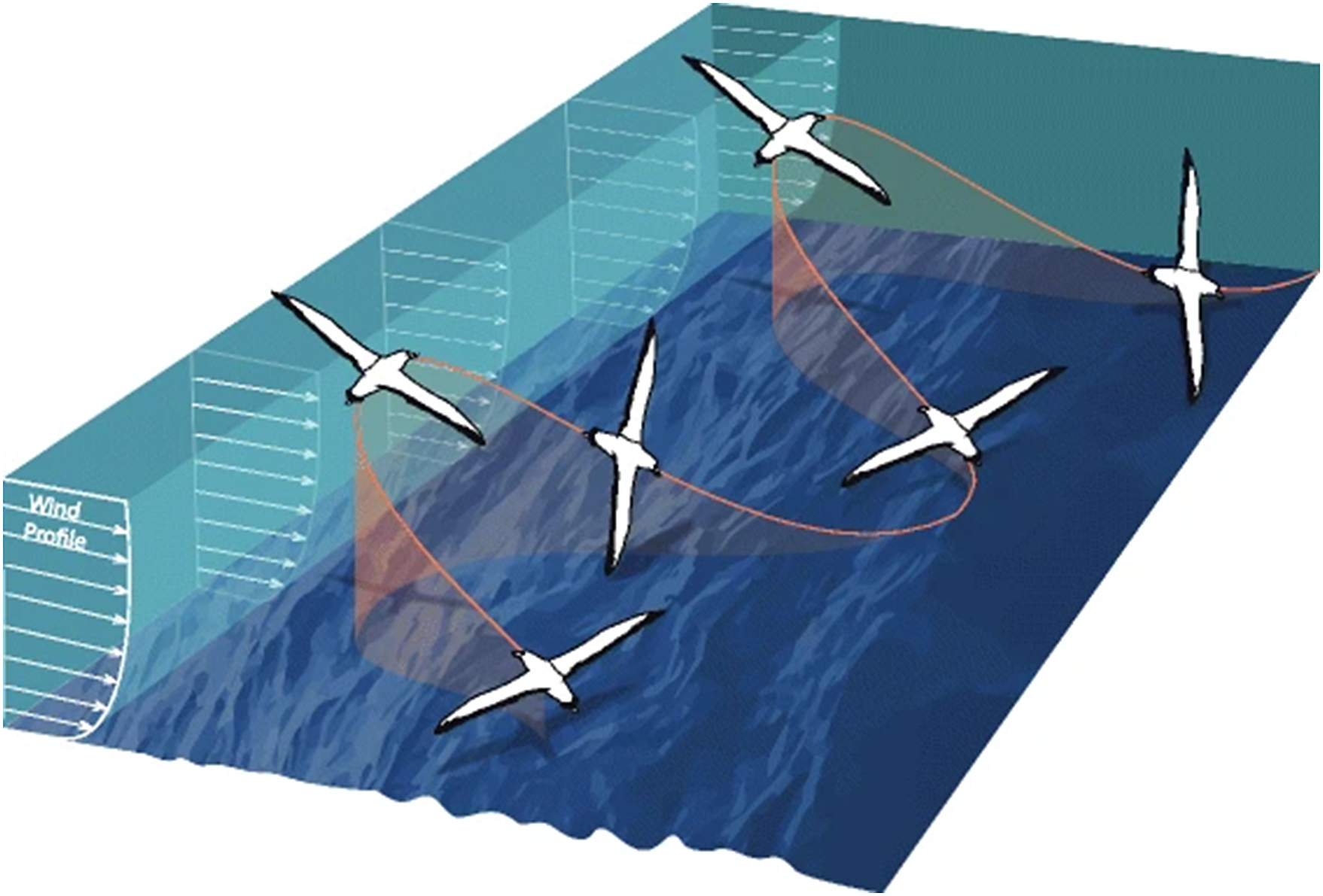
Procellariiformes, such as albatrosses, petrels and shearwaters, utilise dynamic soaring as a flight behaviour to cross vast ocean distances while barely ever flapping their wings (Richardson et al. Reference Richardson, Wakefield and Phillips2018). Dynamic soaring exploits gravity and the vertical gradient in windspeed of the wind-shear layer at the sea surface and provides 80–90% of the total energy required for sustained soaring in Southern Ocean albatrosses (Richardson Reference Richardson2011). Typical dynamic soaring consists of sequential cycles of 5−15 s (Bousquet et al. Reference Bousquet, Triantafyllou and Slotine2017; Sachs Reference Sachs2005; Schoombie et al. Reference Schoombie, Wilson and Ryan2023), within each cycle a bird climbs from close to the sea surface in a wave trough diagonally upwind across the wind-shear layer, upon gaining maximum height it turns c. 90° downwind, descends diagonally across the wind-shear layer into a wave trough, and then turns c. 90° into the wind again (Figure 1; Richardson et al. Reference Richardson, Wakefield and Phillips2018).
Typical S-shaped dynamic soaring cycles. Schematic shows an albatross flying in an across-wind direction through the vertical wind profile. The bird extracts energy from the wind by climbing headed upwind and descending headed downwind. Image reproduced with permission from (Richardson et al. Reference Richardson, Wakefield and Phillips2018).

The exact means of energy gain from dynamic soaring remains an area of active research (Kempton et al. Reference Kempton, Wynn, Bond, Evry, Fayet and Gillies2022; Richardson Reference Richardson2011; Sachs et al. Reference Sachs, Traugott, Nesterova, Dell’Omo, Kümmeth and Heidrich2012), but theory and observations agree that at the lowest point of typical dynamic soaring cycles albatross are consistently very close (<1 m) to the sea surface (Pennycuick Reference Pennycuick1982; Richardson Reference Richardson2011; Sachs et al. Reference Sachs, Traugott, Nesterova, Dell’Omo, Kümmeth and Heidrich2012). We propose to use this “skimming” of the sea surface during the lowest points of dynamic soaring cycles to provide the reference pressure value for altitude calculation using altimeters. This describes a scenario close to optimal altimeter altitude calculation by collecting contemporaneous sea-level reference pressures and pressures at height mere seconds apart and overcomes common altimeter miscalibration associated with short term variation in air pressure associated with the passage of weather systems.
Aims
Here, we introduce a method tailored to address a significant data gap on flight heights in dynamic soaring seabirds such as Procellariiformes. First, we determine whether high sampling-frequency altimeters can be used to detect the vertical magnitude of dynamic soaring cycles. Second, we compare flight heights calculated from altimeters zeroed using dynamic soaring to simultaneously-collected GPS altitudes. Finally, in the absence of independent flight height data, to validate our approach, we compare GPS and altimeter measurements from birds floating on the sea surface to satellite ocean wave data. We use our results to discuss the ability of GPS and altimeter biologgers to measure fine-scale vertical movements in marine conditions and their suitability for seabird flight height estimation.
Methods
Loggers and field attachment
We deployed 11 solar-powered GPS loggers, each with a rear facing barometric pressure sensor and cellular data upload (model ESW400; Cellular Tracking Technologies, LLC, Rio Grande, NJ, USA), on breeding Shy Albatross Thalassarche cauta from Albatross Island namanu rruni off the northwest coast of Tasmania. Loggers were set to record a burst of 1 Hz data for five minutes (“5-min” hereafter) at the start of each hour. Each 5-min burst recorded 300 datapoints of GPS latitude, longitude and altitude, barometric pressure, ambient temperature and instantaneous speed. Nine loggers were deployed at the start of April 2023 (late chick provisioning phase), and two loggers were deployed in late September/early October 2023 (incubation phase). They were attached to the albatross’ mantle feathers using TESA tape and Loctite glue. Each albatross was initially weighed, and deployed loggers (weighing 31–53 g) were less than 3% of the bird’s weight.
Track processing and assigning behaviour
We used the track2KBA R package (Beal et al. Reference Beal, Oppel, Handley, Pearmain, Morera-Pujol and Carneiro2021) to process tracking data into individual trips and remove locations <1 km from the colony. We used the valley of the bimodal distribution of 1 Hz instantaneous GPS groundspeeds as a movement threshold to classify individual latitude-longitude locations as either flying or floating on the sea surface (Weimerskirch et al. Reference Weimerskirch, Bonadonna, Bailleul, Mabille, Dell’Omo and Lipp2002). Our identified speed threshold of 4 ms-1 (Supplementary materials Figure S1) was in agreement with other albatross studies (Yonehara et al. Reference Yonehara, Goto, Yoda, Watanuki, Young and Weimerskirch2016), and used to assign each 5-min data burst into one of three behavioural groups: flying (>95% of datapoints with speed >4 ms-1), floating on the sea surface (>95% of datapoints with speed ≤4 ms-1), or take off/landing (<95% dominance of flying or floating datapoints).
Detecting dynamic soaring vertical movements
To proof our proposed use of dynamic soaring to improve altimeter flight height estimation, we first determined whether the vertical component (altitude) of dynamic soaring cycles could be detected via changes in barometric pressure. Given albatross floating on the sea surface can record the vertical magnitude and periodicity of ocean waves with GPS biologgers sampling at 6 Hz (Uesaka et al. Reference Uesaka, Goto, Yonehara, Komatsu, Naruoka and Weimerskirch2022), we considered that 1 Hz GPS and barometric pressure sampling should be sufficient to detect the larger vertical magnitude and periodicity of dynamic soaring cycles. To test this, we segmented raw GPS altitude and barometric pressure timeseries into individual dynamic soaring cycles using an automatic timeseries peak detection algorithm in the pracma R package (Borchers Reference Borchers2023). We ran the peak detection algorithm in a similar manner to Schoombie et al. (Reference Schoombie, Wilson and Ryan2023), by first smoothing the time series (3-sample rolling mean) and then specifying a minimum duration between successive dynamic soaring peaks (5 seconds). To further separate out noise, we additionally specified that dynamic soaring peaks were preceded by a minimum of two successive increasing steps and followed by a minimum of two successive decreasing steps. If dynamic soaring cycles were detectable in the data then we would expect resultant dynamic soaring segment durations to fall within published values (5−15 second cycle durations; Sachs Reference Sachs2005, Bousquet et al. Reference Bousquet, Triantafyllou and Slotine2017, Schoombie et al. Reference Schoombie, Wilson and Ryan2023). If this was the case for both GPS and pressure timeseries then this was indicative of true detection, given the fundamental differences in between how the two sensors measure vertical height.
Estimating flight height
GPS altitude values were provided by loggers relative to mean sea level. However, we determined from known altitudes at the Albatross Island breeding colony, and instances of birds floating on the sea surface, that all loggers constantly overestimated altitude by an average of 9 m (see Supplementary materials for detail). As per Schaub et al. (Reference Schaub, Millon, De Zutter, Buij, Chadœuf, Lee and Mionnet2023), we interpreted this as a discrepancy with the geoid model used by the manufacturer and applied a minus 9 m correction to all GPS altitudes.
Altimeters estimate flight height above sea level (h) using the barometric formula (Berberan-Santos et al. Reference Berberan-Santos, Bodunov and Pogliani1997):

where h = altitude (m); k = universal gas constant for air (8.31432 N m mol−1 K−1); T = temperature (K) recorded by the logger; m = molar mass of air (0.0289644 kg mol−1); g = acceleration due to gravity (9.80665 ms−2); P0 = the reference atmospheric pressure (Pa) at sea level (0 m); P= atmospheric pressure (Pa) at height h (m). We propose zeroing altimeters with the lowest points of dynamic soaring cycles, which is when albatrosses the skim the sea surface, to set P0 in the barometric equation. We are confident that each 5-min data burst contains at least some dynamic soaring behaviour, and therefore low points of cycles at sea level to set P0, as albatrosses spend 74–95% of flight time dynamic soaring (Conners et al. Reference Conners, Michelot, Heywood, Orben, Phillips and Vyssotski2021; Sakamoto et al. Reference Sakamoto, Takahashi, Iwata, Yamamoto, Yamamoto and Trathan2013; Schoombie et al. Reference Schoombie, Wilson and Ryan2023) and continuous flapping bouts last on average 1.9 minutes (Conners et al. Reference Conners, Michelot, Heywood, Orben, Phillips and Vyssotski2021).
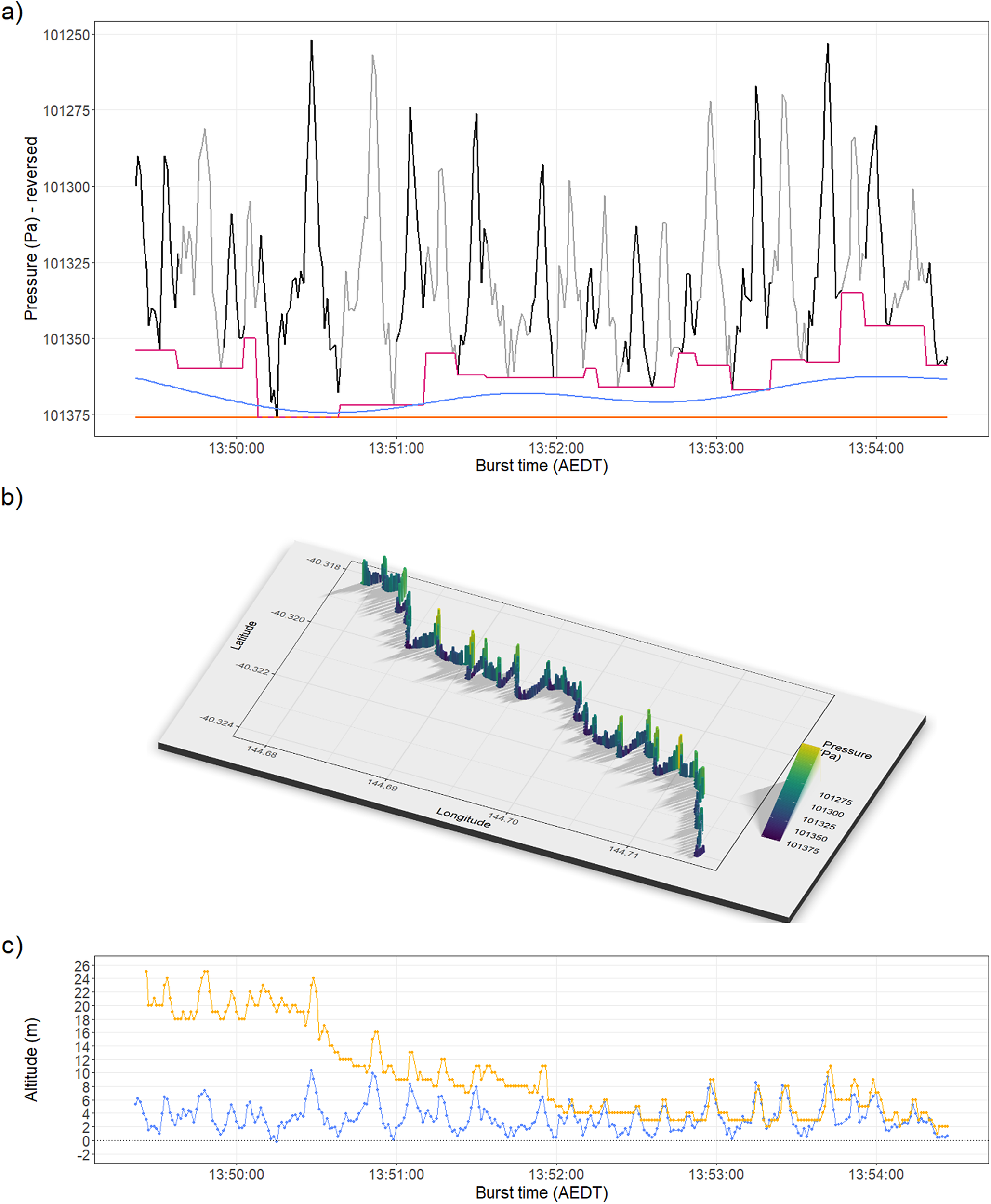
However, the portions of flight spent flapping and the likelihood that not all dynamic soaring cycles conform to the typical theoretical model (e.g. energy for soaring is likely supplemented by updrafts over waves; Richardson et al. Reference Richardson, Wakefield and Phillips2018) means that we should not assume albatross skim the sea surface every 5–15 seconds (as per typical dynamic soaring). To accommodate this uncertainty around P0 and its’ impact on barometric altitude calculation, we modelled three dynamic soaring scenarios for each 5-min data burst (Figure 2a). An upper scenario assumed that only the highest pressure value within each 5-min burst represented true sea level (P0) and all other pressure values represented the bird flying some height above sea level. A lower scenario assumed every dynamic soaring cycle skimmed the sea surface, and flight heights were calculated independently for each cycle using the cycle-specific maximum P0 value. A central scenario was estimated by fitting a Generalised Additive Model (GAM) between the upper and lower scenarios, allowing P0 a degree of flexibility across each 5-min burst (spline fitted with one knot per minute in the mgcv R package; Wood Reference Wood2011). GAMs were formulated for each burst separately, using midpoints between upper and lower scenario pressure values as the dependant variable and time as the predictor variable. Fitted values returned by each GAM provided P0 values for the central scenario. Flight heights were calculated using each of the three scenarios, while the difference between the upper and lower scenarios were used to express the plausible range of flight height estimates under the altimeters-zeroed-with-dynamic-soaring methodology.
An example 5-min data burst from a GPS-altimeter biologger on a flying Shy Albatross (a) Shows the timeseries of raw altimeter pressure values, with individual dynamic soaring cycles segmented (black-grey alternation). Three lines provide different representations of estimated sea level reference pressure (P0) for altitude calculation: orange assumes an upper scenario where sea level pressure is provided by the single maximum pressure value; pink assumes a lower scenario where every dynamic soaring cycle meets the sea surface, with its’ own P0 value; and blue shows the central scenario between the upper and lower scenarios, allowing P0 a degree of flexibility across each 5-min burst; (b) shows the same pressure data as a), visualised with co-sampled GPS locations to show movement in 3D; (c) Shows the same 5-min burst, with central-scenario pressure values converted to altitude above mean sea level (blue), and compared to co-sampled GPS altitude (yellow).

Figure 2. Long description
The figure consists of three vertically stacked panels labeled a, b, and c.
Panel a is a line graph with the x-axis Burst time A E D T from 13 50 00 to 13 54 00 and the y-axis Pressure P a reversed from 101250 at the top to 101375 at the bottom. A jagged line alternates between black and grey segments representing dynamic soaring cycles. Three reference lines are present. A flat orange line at the bottom represents the upper scenario. A stepped pink line follows the local pressure maxima of each cycle. A smooth blue wave oscillates between the pink and orange lines.
Panel b is a 3 D perspective plot showing movement across Latitude and Longitude. The flight path is represented by a series of vertical bars colored by a gradient from purple high pressure to yellow low pressure. The path moves diagonally from the top-left toward the bottom-right of the grid, with a shadow cast on the base plane.
Panel c is a line graph with the same x-axis as panel a. The y-axis is Altitude in meters ranging from negative 2 to 26. Two data series are shown. A yellow line with square markers fluctuates between 2 and 26 meters, showing a general downward trend in peak height over time. A blue line with circular markers fluctuates between 0 and 10 meters, representing the central scenario altitude. A horizontal dotted line marks the 0 meter sea level baseline.
An alternative altimeter method for seabirds uses pressure values recorded by birds when floating on the water to set the reference atmospheric pressure for sea level (P0), allowing recalibration of the barometric equation each time a bird rests (Cleasby et al. Reference Cleasby, Wakefield, Bearhop, Bodey, Votier and Hamer2015). If birds do not float on the water regularly, this method can be further improved by integrating hourly satellite data (Johnston et al. Reference Johnston, Thaxter, Boersch-Supan, Davies, Clewley and Green2023). However, even with satellite data augmentation, there are limitations to how widely the ‘floating on water’ method can be applied. Considering that our data were collected in hourly 5-min data bursts rather than continuously at 1-second, 10-second, 2-minute or 10-minute interval (Cleasby et al. Reference Cleasby, Wakefield, Bearhop, Bodey, Votier and Hamer2015; Johnston et al. Reference Johnston, Thaxter, Boersch-Supan, Davies, Clewley and Green2023), our ability to regularly record floating bouts was limited. Indeed, 5-min data bursts classified as flying were on average 6.8 (95% CI: 5.4, 8.9) hours from the nearest recordings of floating behaviour (after excluding floating bouts >1 day away; Johnston et al. Reference Johnston, Thaxter, Boersch-Supan, Davies, Clewley and Green2023). Given the decay in the precision of height estimates as the time interval (Δt) between observations of P0 and P increases (e.g. ±1 m at Δt of 11.5 minutes, while ±7.3 m at Δt of 2.7 hours; Cleasby et al. Reference Cleasby, Wakefield, Bearhop, Bodey, Votier and Hamer2015) due to the effect of weather, atmospheric tides etc, we decided that our data sampling strategy introduced too much error to the ‘floating on water’ method and it was not used.
Validation of vertical movements from floating birds against satellite wave data
With no independent flight height data available for validation, we instead tested whether the vertical height and periodicity of ocean waves could be accurately estimated from GPS and altimeter sensors. We subset our data to bursts where birds were classified as floating on the water and performed zero-crossing analyses to extract significant wave height (average wave height of the top one-third highest waves) and average periodicity per burst in the oceanwaves R package (Miller & Neumeier Reference Miller and Neumeier2021). We then obtained a corresponding value from satellite for significant wave height and average wave periodicity using the European Centre for Medium Range Weather Forecasts (ECMWF) reanalysis model ‘ERA5’. Hourly ERA5 wave data were available at 30 km spatial resolution and extracted for using the coordinates and timestamp of each burst with the Movebank Env-DATA system (Dodge et al. Reference Dodge, Bohrer, Weinzierl, Davidson, Kays and Douglas2013).
Statistical analyses
All analyses were carried out in R version 4.3.1 (R Core Team 2023). To compare dynamic soaring cycle duration between altimeter and GPS sensors, we used a Mann-Whitney U test. To compare between flight heights from GPS altitude and altimeters, we used paired Wilcoxon tests. To test for agreement between biologger and satellite ERA5 data when estimating ocean wave height and periodicity, we used Pearson’s correlations.
Results
Deployment and data return
Of the 11 loggers deployed only three returned data, with durations: 01–04 April 2023 and 01–18 April 2023 (representing late chick provisioning phase); and 29 September–02 October 2023 (representing incubation phase). The three loggers returned 245 5-min bursts of co-sampled GPS-pressure data obtained from birds >1 km from the colony. Of these bursts, we removed 86 that showed erroneous pressure readings consistent with the pressure sensor being submerged or swamped with seawater, and a further three with poor GPS signal (>50% of altitudes >1,000m). Of the remaining bursts we classified 50 as floating on the water, 85 as flying, and 21 as takeoff/landing.
Pressure sensors can detect dynamic soaring
We found clear dynamic soaring cycles occurring simultaneously in raw barometric pressure and GPS altitude timeseries (Figure 2). When plotted in 3D, with co-sampled GPS latitude and longitude, vertical oscillations clearly matched the spatial dynamic soaring cycles. Average dynamic soaring cycle durations recorded by altimeters were approximately half a second longer than those reported by GPS (altimeter 10.4 ± 4.94 s; GPS 9.81 ± 5.08 s; Mann-Whitney U, W =76,295, P = <0.0001), with both within reported albatross range (5–15 s). GPS altitude struggled to hold a steady reference altitude (e.g. sea level) during bursts. In some, the GPS accuracy appeared to improve over the 5-min burst and flight heights from the two sensors converged in the later minutes (e.g. Figure 2c), but in other bursts GPS altitude fluctuated above and below 0 m for minutes at a time (See Supplementary material Figure S3).
Comparison of flight heights from altimeter and GPS
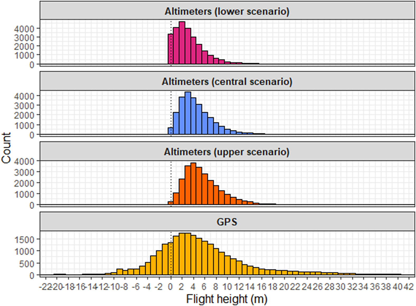
The central altimeter scenario and GPS altitude agreed on average Shy Albatross flight heights of c.4 m (Figure 3; Table 1). The mean and median flight heights from GPS occurred between the central and upper altimeter scenarios (Table 1), with the median flight heights from altimeters all differing significantly from GPS (paired Wilcoxon: GPS-altimeter lower scenario V = 198,704,999, P = <0.0001; GPS-altimeter central scenario V = 167,397,686, P = <0.0001; GPS-altimeter upper scenario V = 138,154,406, P = <0.0001). GPS flight heights showed high variance around the mean and conformed to a normal distribution, whereas altimeter flight heights showed lower variances and had right skewed distributions (skewness >1; Table1), due to greater concentrations of datapoints on the left side of their distributions (flight heights <5 m) and longer tails on the right.
Histogram of flight heights estimated by altimeter and GPS from 5-min data bursts recorded by Shy Albatross while flying.

Figure 3. Long description
The x-axis represents Flight height in meters, ranging from negative 22 to positive 42. The y-axis represents a count of datapoints, ranging from 0 to 4000. A vertical dotted line marks the zero point on the x-axis.
Four histograms are plotted:
* Altimeters lower scenario (magenta): The tallest, narrowest peak reaching approximately 4000 datapointsy at 2 meters.
* Altimeters central scenario (blue): A slightly lower peak reaching approximately 4000 datapoints at 3 meters.
* Altimeters upper scenario (orange): A peak reaching approximately 4000 datapoints at 4 meters.
* G P S Altitude (yellow): The lowest and broadest curve, with a peak around 1600 datapoints at 3 meters and a long tail extending into higher positive values and negative values down to negative 10 meters.
The altimeter-based histograms are tightly clustered between 0 and 15 meters, while the G P S data shows significantly higher variance.
Comparison of summary statistics of flight heights estimated by altimeter and GPS from 5-min data bursts recorded by Shy Albatross whilst flying.

Table 1. Long description
The table contains eight columns: Method, Mean plus or minus standard deviation, Median, Minimum, Maximum, 25th percentile, 75th percentile, and Distribution skewness. All height values are in meters.
* Altimeter lower scenario: Mean 3.23 plus or minus 2.70, Median 2.67, Min 0, Max 26.1, 25th percentile 1.26, 75th percentile 4.55, Skewness 1.46.
* Altimeter central scenario: Mean 4.48 plus or minus 2.89, Median 3.91, Min 0, Max 26.1, 25th percentile 2.41, 75th percentile 5.97, Skewness 1.23.
* Altimeter upper scenario: Mean 5.61 plus or minus 3.24, Median 4.97, Min 0, Max 26.1, 25th percentile 3.28, 75th percentile 7.32, Skewness 1.09.
* G P S altitude: Mean 5.10 plus or minus 9.72, Median 4, Min minus 63, Max 89, 25th percentile 0, 75th percentile 9, Skewness 0.0607.
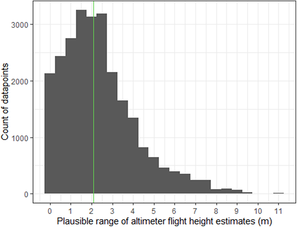
As a measure of uncertainty, we calculated the difference in flight heights between the upper and lower altimeter scenarios to give the plausible range (minimum and maximum) for each flight height under the altimeters-zeroed-with-dynamic-soaring methodology (Figure 4). The median plausible range was 2.1 m, varying from 0–10.8 m. We also found some logger-specific variation, with median plausible ranges of 2.6, 2.1 and 1.8 m respectively for the three loggers (Supplementary material Figure S2).
Plausible range of each flight height under the altimeters-zeroed-with-dynamic-soaring methodology. Plausible range is the difference between flight heights from our upper and lower scenarios. Green line shows the median.

Figure 4. Long description
The X-axis is labeled Plausible range of altimeter flight height estimates in meters m, with a scale from 0 to 11. The Y-axis is labeled Count of datapoints, with a scale from 0 to 3000. The data is presented as a dark gray histogram.
* The distribution begins at 0 and rises sharply to a peak between 1 and 2 meters, where the count exceeds 3000.
* A vertical green line marks the median at approximately 2.1 meters.
* Following the peak, the counts decrease in a right-skewed tail.
* The frequency drops below 1000 by the 5-meter mark and continues to taper off toward 10 meters.
* A very small isolated bar is visible at the 11-meter mark.
Validation of vertical movements from floating birds against satellite ERA5 wave data
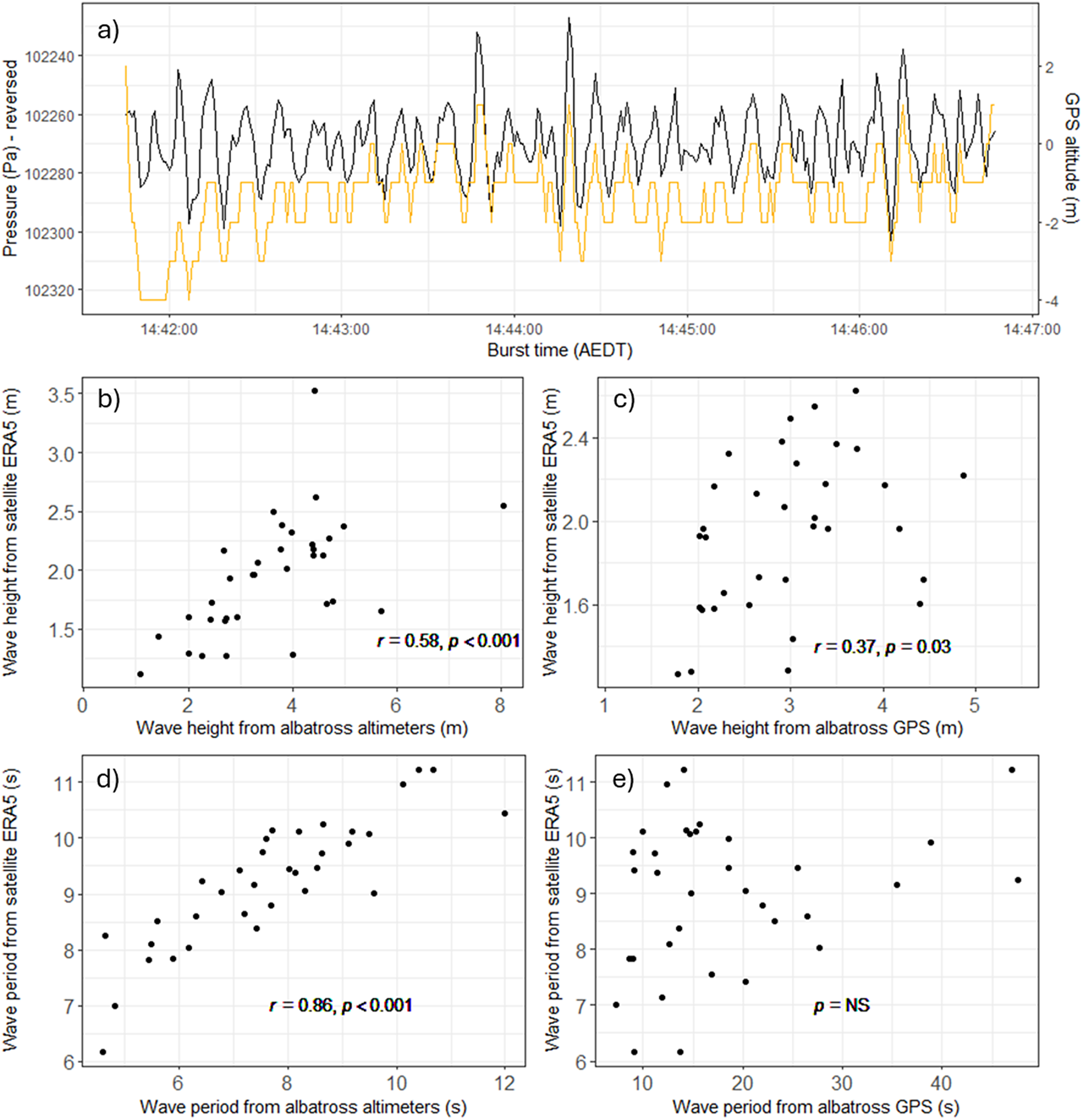
While albatross floated on the sea surface, the vertical signals of waves were clear in altimeter and GPS altitude timeseries (Figure 5a). However, altimeters were better correlated with independent satellite ERA5 data than GPS when estimating significant wave height and wave periodicity (Figure 5b–e).
a) Shows an example 5-min data burst recorded by a biologger on a Shy Albatross while it sat on the sea surface. Altimeter (black) and GPS (yellow) timeseries of raw data show recording of ocean waves by both sensors. Subfigures b) – e) show significant wave height and average wave periodicity as estimated concurrently from satellite ERA5 data and from albatross-borne altimeter and GPS sensors.

Figure 5. Long description
Panel a is a line graph showing a 5-minute data burst. The x-axis is Burst time in A E D T from 14:42:00 to 14:47:00. The left y-axis is Pressure in Pa - reversed, ranging from 102240 to 102320, plotted as a black line representing Altimeter data. The right y-axis is G P S altitude in meters, ranging from -4 to 2, plotted as a yellow line. Both lines show high-frequency oscillations corresponding to ocean waves.
Panels b through e are scatter plots comparing albatross-borne sensor data on the x-axis to satellite E R A 5 data on the y-axis.
Panel b: Wave height from albatross altimeters in meters (x) versus Wave height from satellite E R A 5 in meters (y). Data shows a positive correlation with r = 0.58 and p < 0.001.
Panel c: Wave height from albatross G P S in meters (x) versus Wave height from satellite E R A 5 in meters (y). Data shows a weak positive correlation with r = 0.37 and p = 0.03.
Panel d: Wave period from albatross altimeters in seconds (x) versus Wave period from satellite E R A 5 in seconds (y). Data shows a strong linear increase with r = 0.86 and p < 0.001.
Panel e: Wave period from albatross G P S in seconds (x) versus Wave period from satellite E R A 5 in seconds (y). Data is highly scattered with p = N S, indicating no significant correlation.
Discussion
We present the first flight heights from bird-borne altimeters zeroed using dynamic soaring behaviour. This new altimeter method agreed with GPS altitude on average Shy Albatross flight heights of c.4 m, but altimeters showed a clearer right skew to the flight height distribution, important for determining the amount of time spent in higher altitudes also occupied by offshore wind turbine blades. While the three birds tracked in this pilot study may not provide a representative sample of Shy Albatross flight heights, our method is widely applicable to dynamic soaring seabirds (e.g. >100 species of albatrosses, petrels and shearwaters).
We succeeded in our aim of using altimeters to detect the vertical movements of dynamic soaring but demonstrate that high-frequency GPS altitude can also do so. GPS and altimeters use fundamentally different methods to estimate altitude, and their consensus on recording dynamic soaring cycles provides an independent validation of complimentary methods. Further independent validation of the ability of altimeters to detect fine scale vertical movement comes from their measurement of wave height and periodicity while birds floated on the sea surface, which better aligned with satellite ERA5 wave data than GPS altitudes were. The tiny battery requirement of altimeter sensors compared to GPS sensors (Schaub et al. Reference Schaub, Millon, De Zutter, Buij, Chadœuf, Lee and Mionnet2023), offers equivalently higher altitude sampling frequencies or longer deployment durations in biologgers.
Seabird flight heights from GPS altitude
The GPS altitudes we recorded were able to clearly track dynamic soaring vertical movements but struggled to maintain a constant altitudinal baseline throughout each 5-min burst, resulting in reported dynamic soaring cycles and wave heights being both above and below sea level (Supplementary material Figure S3). By contrast, GPS biologgers deployed onto floating seabirds by Uesaka et al. (Reference Uesaka, Goto, Yonehara, Komatsu, Naruoka and Weimerskirch2022) accurately measured wave height, likely facilitated by their 6 Hz sampling rate compared to the 1 Hz rate used here. Improvements in GPS technology, such as new satellite constellations and regional augmentation networks, may yield more accurate GPS altitude (Montenbruck et al. Reference Montenbruck, Steigenberger, Prange, Deng, Zhao and Perosanz2017), and future studies should focus efforts on high-frequency sampling (>1 Hz). This would allow improved flight heights to be calculated by subtracting accurate recordings of real sea level height (rather than GPS geoid) when birds float on the water from GPS altitudes recorded when birds fly (e.g. Adams et al. Reference Adams, Felis and Czapanskiy2020). Our GPS altitude data were normally distributed, with error likely caused by a combination of orbital shifts, satellite clock shifts, and the ionosphere (Olynik et al. Reference Olynik, Petovello, Cannon and Lachapelle2002), and it should be acknowledged that applicable state-space modelling approaches exist to statistically account for systematic and random GPS error in seabird flight heights (Davies et al. Reference Davies, Boersch-Supan, Clewley, Humphreys, O’Hanlon and Shamoun-Baranes2024; Johnston et al. Reference Johnston, Thaxter, Boersch-Supan, Davies, Clewley and Green2023; Ross-Smith et al. Reference Ross-Smith, Thaxter, Masden, Shamoun-Baranes, Burton and Wright2016). These approaches assume true seabird flight heights originate from a log-normal (or similar) distribution, but are observed imperfectly by the GPS biologger. Data on seabird behaviour (e.g. flying/floating) and GPS fix quality (e.g. number of satellites) can be included to account for systematic and random error respectively.
Seabird flight heights from barometric pressure
We have shown that pressure sensors have the ability to record accurate flight heights in dynamic soaring seabirds, validating their accurate measurement of sinusoidal drone movements (Lato et al. Reference Lato, Stepanuk, Heywood, Conners and Thorne2022). However, pressure sensors are more sensitive to their surrounding environment than GPS (Péron et al. Reference Péron, Calabrese, Duriez, Fleming, García-Jiménez and Johnston2020), which can introduce uncertainty into altitude calculation. As a metric of uncertainty, we calculated the typical plausible range of each flight height under our methodology (difference between upper and lower scenarios) as being 2.1 m and consider this to include multiple sources of error. For example, differences in height between an albatross skimming the sea surface at a wave crest compared to a wave trough and differences in albatross orientation relative to logger position - dynamic soarers often roll their bodies perpendicular to the sea surface, such that back-mounted loggers could be 1.15 m higher than the lower wingtip skimming the sea surface (Shy Albatross mean wingspan of 2.3 m; Hedd Reference Hedd1999). Further error was likely introduced from micro-scale weather and dynamic ocean phenomena, for example occasional 5-min data bursts showed a trend in their baseline pressure as if birds passed through local (c. minute long) pressure gradients (Supplementary material Figure S3-S4). These examples likely contributed to larger plausible range values calculated for some flight heights (Figure 4). Our lower and upper scenarios help understand the scale of altimeter uncertainty associated with our methodology and have potential application (e.g. using upper scenario flight heights under the precautionary principle). However, the methods used to specify these scenarios (automatic segmentation of dynamic soaring cycles) and the central scenario (GAM parameters) could be further refined. We recommend additional research to validate the results of our three-bird pilot study. For example, data collection over a broader sample of individuals and in a wider range of environmental conditions or deployment of altimeter biologgers on drones, equipped with LiDAR for independent, accurate altitude measurement, carefully flown to mimic dynamic soaring. We also note the potential application of state-space modelling approaches developed for seabird GPS data, to also statistically account for multiple error sources in altimeter flight heights (Bogdanova et al. Reference Bogdanova, Wischnewski, Cleasby, Whyte, Regan and Gunn2021; Johnston et al. Reference Johnston, Thaxter, Boersch-Supan, Davies, Clewley and Green2023).
Procellariiform flight heights and collision risk
Current flight height estimates for Procellariiformes are extremely scarce, with a recent literature review returning only one or two datapoints on mean flight height for 21 species (Miller et al. Reference Miller, Petrovic and Clarke2025). Given the sensitivity of collision risk models to flight height (e.g. Lesser Black-backed Gull Larus fuscus collision risk modelling using flight heights from altimeters gave 17 more collisions per month compared to flight heights from GPS altitude; Johnston et al. Reference Johnston, Thaxter, Boersch-Supan, Davies, Clewley and Green2023), it is important that not only are Procellariiform flight height data gaps filled, but that they are filled by accurate data. In this regard, our pilot study makes a timely contribution by demonstrating how dynamic soaring flight behaviour recorded by low-power altimeters can produce flight height estimates that are comparable or better than those estimated via GPS, with the method widely applicable to dynamic soaring seabirds (>100 Procellariiform species). Ultimately, altimeter and GPS biologgers should be used complimentarily to overcome platform-specific error sources, and thereby maximise the accuracy of resultant Procellariiform flight heights.
Supplementary material
The supplementary material for this article can be found at http://doi.org/10.1017/S095927092610063X.
Acknowledgements
We acknowledge and pay respect to Palawa (Tasmanian Aboriginal people) as the Traditional Owners of Lutruwita/Tasmania. We remember and honour their Elders, past and present, and acknowledge Palawa as the continuing custodians of the rich cultural heritage of Lutriwita. The Marine Conservation Program (MCP) of The Department of Natural Resources and Environment Tasmania (NRE Tas) undertake annual monitoring of Shy Albatross populations, maintaining long-term population, demography, and telemetry databases. MCP access the Albatross Island Nature Reserve under an ‘Authority to Conduct an Activity on Reserved Land’ pursuant to Regulation 28 of the National Parks and Reserves Management Regulations 2019 granted by the Tasmania Parks and Wildlife Service (1/7/2022–30/6/2023; 1/7/2023–30/6/2024). On-island logger deployments were undertaken during MCP annual monitoring trips to Albatross Island funded by the Department of Climate Change, Energy, the Environment and Water and NRE Tas. Field work and logger deployments completed under Sheryl Hamilton’s NRE Tas staff permits (Listed Taxon Permit 2201521/1 and Special Purposes Wildlife Permit 2201519/1) and the NRE Tas Animal Ethics Committee approved Standard Operating Procedure Monitoring the at-sea distribution and behaviour of seabirds in Tasmania and Macquarie Island using telemetry devices. We thank Julie McInnes, Marcus Salton, Clare Lawrence, Mike Double and Alexa Wolfs for field assistance, Sam Thalmann and Philipp Boersch-Supan for helpful comments on the manuscript, and two reviewers whose input improved the final product.
Data accessibility
Code required to perform analyses is publicly available at: https://github.com/lark-gorilla/flight_heights. The raw tracking data is freely available at Monash Bridges (https://doi.org/10.26180/33829756).
Author contribution
MGRM and RHC wrote the manuscript with support from SAH. RHC and MGRM conceptualised the study. SAH and MGRM conducted fieldwork. MGRM analysed the data. All authors read and approved the final manuscript.
Competing interest
The authors declare no conflict of interest. Rohan Clarke receives funding from the Australian Research Council, the Australian Department of Energy, Environment, and Climate Action, Zoos Victoria, and the offshore energy sector in Australia. The research reported here was funded directly by Monash University.



 Open access

