
1. Introduction
Understanding heat and mass transport processes is important for: comprehending natural phenomena, such as combustion and chemical reactions; finding solutions to real-world problems, such as pollutant dispersion; advancing earth-related scientific fields, such as oceanography and atmospheric science. In many commonly encountered situations, particularly in industrial and geophysical flows, the velocity field generates fluctuations in a scalar field and vice versa, complicating the flow fields. If, however, the effects of the scalar field on the velocity field can be neglected for small temperature fluctuations or low solute concentrations, the scalar is said to be passive. The study of passive scalars is a major subject in fluid turbulence (Gotoh & Yeung Reference Gotoh and Yeung2012), because it provides a simple model of turbulent mixing (Shraiman & Siggia Reference Shraiman and Siggia2000; Warhaft Reference Warhaft2000; Sreenivasan Reference Sreenivasan2018). While the simplest configuration is a homogeneous isotropic scalar subjected to homogeneous isotropic turbulence, the real-world practical problems possess a mean scalar gradient. Thus, the second simplest configuration – a passive scalar with a mean gradient, subjected to homogeneous isotropic turbulence – is the subject of the present study. In the context of grid turbulence, such a passive scalar has previously been investigated in experiments on temperature fluctuations (Tavoularis & Corrsin Reference Tavoularis and Corrsin1981a,Reference Tavoularis and Corrsinb; Sirivat & Warhaft Reference Sirivat and Warhaft1983; Mydlarski & Warhaft Reference Mydlarski and Warhaft1998) and may be regarded as an idealised model of a scalar mixing layer (Suzuki et al. Reference Suzuki, Nagata, Sakai and Ukai2010; Ito et al. Reference Ito, Watanabe, Nagata and Sakai2016).
According to Kolmogorov (Reference Kolmogorov1941a,Reference Kolmogorovb), Obukhov (Reference Obukhov1949) and Corrsin (Reference Corrsin1951), at sufficiently small scales there is a certain kind of universality at high Reynolds and Péclet numbers. The central assumption of Kolmogorov–Obukhov–Corrsin theory is that small scales are statistically independent of large scales throughout the cascade process. However, this assumption remains controversial for a passive scalar in the presence of a mean scalar gradient (Warhaft Reference Warhaft2000). Such a gradient acts as a source of the passive scalar, giving rise to a mean scalar flux and making the passive scalar field anisotropic.
This remarkable violation of local isotropy has been pointed out in the literature (Mydlarski & Warhaft Reference Mydlarski and Warhaft1998; Warhaft Reference Warhaft2000). For instance, it has been shown by means of experiment (Mydlarski & Warhaft Reference Mydlarski and Warhaft1998) and direct numerical simulation (DNS) (Overholt & Pope Reference Overholt and Pope1996) that the local isotropy measured by the ratio of the mean squared scalar gradient in different directions is independent of Reynolds number. Furthermore, non-zero odd-order moments of scalar gradient have also been observed in both experiments (Mydlarski & Warhaft Reference Mydlarski and Warhaft1998) and DNSs (Pumir Reference Pumir1994; Overholt & Pope Reference Overholt and Pope1996; Yeung, Xu & Sreenivasan Reference Yeung, Xu and Sreenivasan2002). Persistent skewness has been observed even in passive scalars advected by delta-correlated Gaussian velocity (Holzer & Siggia Reference Holzer and Siggia1994); this implies that the anisotropy does not strongly depend on the turbulent structures. Therefore, the assumption of local isotropy in passive-scalar turbulence is still questionable, and inclusion of anisotropy in theoretical analysis is important not only for the better understanding of turbulent mixing, but also for accurate subgrid modelling in large eddy simulations. However, numerous questions on the subject remain without clear answers – see the review by Warhaft (Reference Warhaft2000).
Whereas much research has been conducted on persistent anisotropies measured using odd-order moments (Pumir Reference Pumir1994; Pumir, Shraiman & Siggia Reference Pumir, Shraiman and Siggia1997; Mydlarski & Warhaft Reference Mydlarski and Warhaft1998; Bos Reference Bos2014) and anomalous scaling exponents of structure functions in the inertial convective range (Kraichnan Reference Kraichnan1994; Shraiman & Siggia Reference Shraiman and Siggia2000; Gotoh, Watanabe & Suzuki Reference Gotoh, Watanabe and Suzuki2011), the smaller scales are often (but not always) of limited practical importance because the transport of passive scalars is usually controlled by the larger scales. In practical problems involving turbulence modelling and quantitative evaluation of mixing, accurate descriptions of lower-order statistics are required more than those of higher-order moments.
This is consistent with the spirit of spectral closure theory, the purpose of which is to derive equations of spectra from first principles, and the resulting closure equations enable us to assess statistical quantities based on the spectra. Closure theories have been developed under various approximations, e.g. eddy-damped quasi-normal Markovian (EDQNM) (Briard et al. Reference Briard, Gomez, Sagaut and Memari2015), test-field model (Newman & Herring Reference Newman and Herring1979; Herring et al. Reference Herring, Schertzer, Lesieur, Newman, Chollet and Larcheveque1982), local energy-transfer (McComb, Filipiak & Shanmugasundaram Reference McComb, Filipiak and Shanmugasundaram1992), Lagrangian history direct interaction approximation (Kraichnan Reference Kraichnan1968), Lagrangian direct interaction approximation (LDIA) (Goto & Kida Reference Goto and Kida1999; O'Gorman & Pullin Reference O'gorman and Pullin2005) and Lagrangian renormalised approximation (LRA) (Kaneda Reference Kaneda1986; Gotoh, Nagaki & Kaneda Reference Gotoh, Nagaki and Kaneda2000). Owing to advances in high-performance computing technologies, turbulent flows with high Reynolds and Péclet numbers can now be analysed, so that closure has a different role than it had a few decades ago, when many comparative studies of closures were conducted (Newman & Herring Reference Newman and Herring1979; Herring et al. Reference Herring, Schertzer, Lesieur, Newman, Chollet and Larcheveque1982). However, closures may still be advantageous in predicting the asymptotic behaviour of turbulence (which is difficult even with current computational technologies), and in cases that require many ensemble averages (e.g. in parametric studies). In such cases, the small-scale turbulent response driven by unsteady forces (Bos, Clark & Rubinstein Reference Bos, Clark and Rubinstein2007) and the decay law of turbulence (Briard et al. Reference Briard, Gomez, Sagaut and Memari2015) are, for example, raised out. In turbulent phenomena where large-scale structure plays an important role, statistical errors cannot be neglected. Indeed, it is often difficult to carry out the large number of DNSs needed for the ensemble average. When one needs to investigate dependence on a parameter such as the Schmidt number, closure provides a way to deepen the phenomenology before performing simulations. Furthermore, closure is useful for theorists identifying mechanisms and for providing further research topics for DNS.
Among the proposed closures, EDQNM is the most popular (Sagaut & Cambon Reference Sagaut and Cambon2008), because it can be used to calculate statistical quantities for finite Reynolds and Schmidt numbers at low computational cost. Recently, it has been extended to the more complex flow fields driven by angle-dependent forcing (Cambon, Mansour & Godeferd Reference Cambon, Mansour and Godeferd1997; Staquet & Godeferd Reference Staquet and Godeferd1998; Favier et al. Reference Favier, Godeferd, Cambon, Delache and Bos2011; Briard, Gomez & Cambon Reference Briard, Gomez and Cambon2016) and unsteady forced turbulence (Bos et al. Reference Bos, Clark and Rubinstein2007). On the other hand, direct interaction approximation (DIA) families have been applied mainly to homogeneous isotropic turbulence and passive scalars (Kraichnan Reference Kraichnan1968; Kaneda Reference Kaneda1981, Reference Kaneda1986; Goto & Kida Reference Goto and Kida1999; Gotoh et al. Reference Gotoh, Nagaki and Kaneda2000); applications to anisotropic turbulence are very limited (Herring Reference Herring1974; Nakayama Reference Nakayama2002; Yoshida, Ishihara & Kaneda Reference Yoshida, Ishihara and Kaneda2003).
While much attention has been paid to closures for homogeneous isotropic passive-scalar fields (Kraichnan Reference Kraichnan1968; Kaneda Reference Kaneda1986; Goto & Kida Reference Goto and Kida1999; Gotoh et al. Reference Gotoh, Nagaki and Kaneda2000), there are only a few studies of ones with a mean scalar gradient (Herr, Wang & Collins Reference Herr, Wang and Collins1996; Bos, Touli & Bertoglio Reference Bos, Touli and Bertoglio2005; O'Gorman & Pullin Reference O'gorman and Pullin2005; Bos Reference Bos2014; Briard et al. Reference Briard, Gomez and Cambon2016). More specifically, the two-time two-point closure has been applied to similarity solutions of the velocity–scalar cospectrum for a wide range of Schmidt numbers (O'Gorman & Pullin Reference O'gorman and Pullin2005), but there has been no attempt to derive the similarity solution of the scalar spectrum. Thus, the effects of the cospectrum on the spectrum are unknown. Furthermore, it was pointed out by Bos et al. (Reference Bos, Touli and Bertoglio2005) that LDIA overestimates the universal constant of the velocity–scalar cospectrum in the inertial subrange; it is presently unclear whether this represents a fundamental failure of LDIA itself. Also, as pointed out by Sagaut & Cambon (Reference Sagaut and Cambon2008) and Bos (Reference Bos2014), the validity of linear theory in anisotropic turbulence is limited, and a nonlinear theory involving triad interactions is necessary. Thus, it is important to investigate the extent to which DIA families are valid for anisotropic turbulence.
On the other hand, the dependence of passive-scalar statistics on the Reynolds and Péclet numbers is not well understood because of the multiple characteristic length scales of velocity and passive scalar fields. Theoretical prediction of these dependences would be valuable for understanding turbulent mixing, and (as mentioned above) closure may be suited for such parametric studies. Furthermore, as little is known regarding the universal features of anisotropy, e.g. large- and small-scale anisotropies and scaling laws of second-order scalar structure functions, it is also valuable to investigate the universal properties of passive-scalar fields in the presence of a mean scalar gradient.
The purposes of this paper are as follows. (i) To approximate the LDIA (Kida & Goto Reference Kida and Goto1997; Goto & Kida Reference Goto and Kida1999) to a single-time two-point spectral closure for passive scalars in the presence of mean scalar gradients using few assumptions and straightforward mathematical procedures. (ii) To validate the proposed closure by comparison with DNS via the fundamental statistical quantities of passive scalars in the presence of mean scalar gradients. In this study, we consider only the case of a Schmidt number equal to unity.
In § 2, spectral closure theory is summarised. In § 2.1, LDIA for a passive scalar in the presence of mean scalar gradients is briefly introduced. Additional information on LDIA and the analytical treatment of triad interactions, including angular dependence, is provided in appendices A and B. In § 2.2 and Appendix C, a mathematical derivation based on single-time Markovianised LDIA is presented.
Two approximate closures are considered in this study; both can be used to calculate statistical quantities. The first is the approximation of LDIA within the framework of single-time two-point closure, where the approximation is done in a straightforward way. However, as pointed out by Cambon, Jeandel & Mathieu (Reference Cambon, Jeandel and Mathieu1981) and Bos et al. (Reference Bos, Touli and Bertoglio2005), the existence of mean-scalar-gradient terms in the nonlinear transfer function makes the level of approximation worse; thus, a second approximation removes these terms. This approximation, a simplification of the first, will be called ‘second closure’. In § 3, the numerical methods used in the DNS and closures are explained.Section 4 discusses the one-point and two-point statistics of passive scalars, e.g. dependence of passive scalar statistics and spectra and structure functions on the Péclet number. Finally, in § 5, the conclusions of the study are presented.
2. Spectral theory
2.1. Lagrangian closure theory
We consider a homogeneous field of velocity  $\boldsymbol {u}$ together with a passive scalar
 $\theta$ with a mean passive scalar gradient
 $\varGamma$. The governing equations are
 $$\begin{gather} \frac{\partial \boldsymbol{u}}{\partial t}+\left(\boldsymbol{u}\boldsymbol{\cdot}\boldsymbol{\nabla}\right)\boldsymbol{u}={-}\boldsymbol{\nabla} p+\nu{\rm \Delta}\boldsymbol{u}+\boldsymbol{f}, \end{gather}$$
 $$\begin{gather}\boldsymbol{\nabla}\boldsymbol{\cdot}\boldsymbol{u}=\boldsymbol{\nabla}\boldsymbol{\cdot}\boldsymbol{f}=0, \end{gather}$$
 $$\begin{gather}\frac{\partial\theta}{\partial t}+\boldsymbol{u}\boldsymbol{\cdot}\boldsymbol{\nabla}\theta=\kappa\varDelta\theta-\varGamma \boldsymbol{u}\cdot\boldsymbol{n}, \end{gather}$$
where  $p$ is the pressure normalised by density,
 $\boldsymbol {f}$ is the forcing term,
 $\nu$ is the kinematic viscosity and
 $\kappa$ is the molecular diffusivity. The unit vector in the direction of the mean passive scalar gradient is defined as
 $\boldsymbol {n}=\boldsymbol {e}_{3}$. Kaneda (Reference Kaneda1981) introduced the Lagrangian position function, defined as
 \begin{equation} \psi\left(\boldsymbol{y},t\mid\boldsymbol{x},s\right)=\delta\left(\boldsymbol{y}-\boldsymbol{z}\left(\boldsymbol{x},s\mid t\right)\right), \end{equation}
where  $\delta (\sim )$ is a three-dimensional Dirac delta function and
 $\boldsymbol {z}(\boldsymbol {x},t\mid s)$ is the position at time
 $t$ of a fluid element that passes
 $\boldsymbol {x}$ at time
 $s$. The Lagrangian position function obeys
 $$\begin{gather} \left(\frac{\partial}{\partial t}+\boldsymbol{u}\left(\boldsymbol{y},t\right)\boldsymbol{\cdot} \boldsymbol{\nabla}_{y}\right)\psi\left(\boldsymbol{y},t\mid\boldsymbol{x},s\right)=0, \end{gather}$$
 $$\begin{gather}\psi\left(\boldsymbol{y},t\mid\boldsymbol{x},t\right)=\delta\left(\boldsymbol{x}-\boldsymbol{y}\right). \end{gather}$$
Based on the Lagrangian position function, the generalised velocity is defined as
 \begin{equation} \boldsymbol{v}\left(\boldsymbol{x},s\mid t\right)=\int {\textrm{d}}\boldsymbol{y}\, \psi\left(\boldsymbol{y},t\mid\boldsymbol{x},s\right)\boldsymbol{u}\left(\boldsymbol{y},t\right), \end{equation}
where it is clear that  $\boldsymbol {v}(\boldsymbol {x},t\mid t)=\boldsymbol {u}(\boldsymbol {x},t)$, and from (2.1a), (2.1b) and (2.3a) that
 \begin{align} \frac{\partial\boldsymbol{v}\left(\boldsymbol{x},s\mid t\right)}{\partial t}&={-}\int {\textrm{d}}\boldsymbol{y}\, \psi\left(\boldsymbol{y},t\mid\boldsymbol{x},s\right)\boldsymbol{\nabla}_{y} p\left(\boldsymbol{y},t\right)+\nu\int {\textrm{d}}\boldsymbol{y}\, \psi\left(\boldsymbol{y},t\mid\boldsymbol{x},s\right)\varDelta_{y}\boldsymbol{u}\left(\boldsymbol{y},t\right) \nonumber\\ &\quad +\int {\textrm{d}}\boldsymbol{y}\, \psi\left(\boldsymbol{y},t\mid\boldsymbol{x},s\right)\boldsymbol{f}\left(\boldsymbol{y},t\right). \end{align}
Much like the generalised velocity, the generalised passive scalar is defined as
 \begin{equation} \theta\left(\boldsymbol{x},s\mid t\right)=\int {\textrm{d}}\boldsymbol{y}\, \psi\left(\boldsymbol{y},t\mid\boldsymbol{x},s\right)\theta\left(\boldsymbol{y},t\right), \end{equation}
where it is clear that  $\theta (\boldsymbol {x},t\mid t)=\theta (\boldsymbol {x},t)$, and from (2.1c) and (2.3a) that
 \begin{equation} \frac{\partial\theta\left(\boldsymbol{x},s\mid t\right)}{\partial t}=\kappa\int {\textrm{d}}\boldsymbol{y}\, \psi\left(\boldsymbol{y},t\mid\boldsymbol{x},s\right)\varDelta_{y}\theta\left(\boldsymbol{y},t\right)-\varGamma \int {\textrm{d}}\boldsymbol{y}\, \psi\left(\boldsymbol{y},t\mid\boldsymbol{x},s\right)u_{3}\left(\boldsymbol{y},t\right). \end{equation}
The closure problem considered here is to determine the subsequent statistical second-order moments, such as  $\langle \boldsymbol {v}(\boldsymbol {x},s\mid t)\boldsymbol {u}(\boldsymbol {y},s)\rangle$,
 $\langle \boldsymbol {u}(\boldsymbol {x},s\mid t)\theta (\boldsymbol {y},s)\rangle$ and
 $\langle \theta (\boldsymbol {x},s\mid t)\theta (\boldsymbol {y},s)\rangle$.
In homogeneous turbulence, closure theory is formulated in terms of the Fourier representation of (2.1a)–(2.7). Hereafter,  $\hat {f}(\boldsymbol {k},t)$ represents the Fourier coefficient of
 $f(\boldsymbol {x},t)$. In Lagrangian closure theories such as LRA and LDIA, the representatives in closed equations are Eulerian correlation, Lagrangian correlation and Lagrangian response functions. These are defined as
 $$\begin{gather} Q_{ij}\left(\boldsymbol{k},t\right)\delta\left(\boldsymbol{k}+\boldsymbol{p}\right)\equiv \left\langle\hat{u}_{i}\left(\boldsymbol{k},t\right)\hat{u}_{j}\left(\boldsymbol{p},t\right)\right\rangle, \end{gather}$$
 $$\begin{gather}F_{i}\left(\boldsymbol{k},t\right)\delta\left(\boldsymbol{k}+\boldsymbol{p}\right)\equiv\left\langle \hat{u}_{i}\left(\boldsymbol{k},t\right)\hat{\theta}\left(\boldsymbol{p},t\right)\right\rangle, \end{gather}$$
 $$\begin{gather}\varTheta\left(\boldsymbol{k},t\right)\delta\left(\boldsymbol{k}+\boldsymbol{p}\right)\equiv \left\langle\hat{\theta}\left(\boldsymbol{k},t\right)\hat{\theta}^{*}\left(\boldsymbol{k},t\right)\right\rangle, \end{gather}$$
 $$\begin{gather}Q_{ij}\left(\boldsymbol{k},t,s\right)\delta\left(\boldsymbol{k}+\boldsymbol{p}\right)\equiv P_{i\alpha}\left(\boldsymbol{k}\right)\left\langle \hat{v}_{\alpha}\left(\boldsymbol{k},s\mid t\right)\hat{u}_{j}\left(\boldsymbol{p},s\right)\right\rangle,\quad t\ge s, \end{gather}$$
 $$\begin{gather}F_{i}^{u\theta}\left(\boldsymbol{k},t,s\right)\delta\left(\boldsymbol{k}+\boldsymbol{p}\right)\equiv P_{i\alpha}\left(\boldsymbol{k}\right)\left\langle \hat{v}_{\alpha}\left(\boldsymbol{k},s\mid t\right)\hat{\theta}\left(\boldsymbol{p},s\right)\right\rangle,\quad t\ge s, \end{gather}$$
 $$\begin{gather}F_{i}^{\theta u}\left(\boldsymbol{k},t,s\right)\delta\left(\boldsymbol{k}+\boldsymbol{p}\right)\equiv \left\langle \hat{\theta}\left(\boldsymbol{k},s\,|\,t\right)\hat{u}_{i}\left(\boldsymbol{p},s\right)\right\rangle,\quad t\ge s, \end{gather}$$
 $$\begin{gather}\varTheta\left(\boldsymbol{k},t,s\right)\delta\left(\boldsymbol{k}+\boldsymbol{p}\right)\equiv\left\langle \hat{\theta}\left(\boldsymbol{k},s\,|\,t\right)\hat{\theta}\left(\boldsymbol{p},s\right)\right\rangle,\quad t\ge s, \end{gather}$$
 $$\begin{gather}G_{ij}\left(\boldsymbol{k},t\mid\boldsymbol{k}',s\right)\equiv P_{i\alpha}\left(\boldsymbol{k}\right)\left\langle \frac{\delta \hat{v}_{\alpha}\left(\boldsymbol{k},s\mid t\right)}{\delta \hat{u}_{j}\left(\boldsymbol{k}',s\right)}\right\rangle,\quad t\ge s, \end{gather}$$
 $$\begin{gather}G_{\theta}\left(\boldsymbol{k},t\mid\boldsymbol{k}'s\right)\equiv \left\langle \frac{\delta \hat{\theta}\left(\boldsymbol{k},s\mid t\right)}{\delta \hat{\theta}\left(\boldsymbol{k}',s\right)}\right\rangle,\quad t\ge s, \end{gather}$$
where the superscript  $*$ denotes the complex conjugate,
 $\delta$ represents the functional derivative and
 $\langle \sim \rangle$ represents an ensemble average. The operator
 $\boldsymbol {P}$ is the solenoidal projector, defined as
 $P_{ij}(\boldsymbol {k})=\delta _{ij}-k_{i}k_{j}/k^{2}$, which plays an important role in LRA and LDIA to eliminate the irrelevant terms in the expansion. Here,
 $\delta _{ij}$ is the Kronecker delta. After lengthy algebra, we have
 $$\begin{gather} \left(\frac{\partial}{\partial t}+2\nu k^{2}\right)Q_{ij}\left(\boldsymbol{k},t\right)=H_{ij}\left(\boldsymbol{k},t\right)+H_{ji}^{*} \left(\boldsymbol{k},t\right)+F_{ij}\left(\boldsymbol{k},t\right)+F_{ji}^{*}\left(\boldsymbol{k},t\right), \end{gather}$$
 $$\begin{gather}\left(\frac{\partial}{\partial t}+\left(\nu+\kappa\right)k^{2}\right)F_{i}\left(\boldsymbol{k},t\right)=H_{i}\left(\boldsymbol{k},t\right)-\varGamma Q_{i3}\left(\boldsymbol{k},t\right), \end{gather}$$
 $$\begin{gather}\left(\frac{\partial}{\partial t}+2\kappa k^{2}\right)\varTheta\left(\boldsymbol{k},t\right)=H\left(\boldsymbol{k},t\right)+H^{*}\left(\boldsymbol{k},t\right)-2\varGamma F_{3}\left(\boldsymbol{k},t\right), \end{gather}$$
 $$\begin{gather}\left(\frac{\partial}{\partial t}+\nu k^{2}\right)Q_{ij}\left(\boldsymbol{k},t,s\right)={-}I_{i\beta} \left(\boldsymbol{k},t,s\right)Q_{j\beta}\left(\boldsymbol{k},t,s\right),\quad t\ge s, \end{gather}$$
 $$\begin{gather}\left(\frac{\partial}{\partial t}+\nu k^{2}\right)F_{i}^{u\theta}\left(\boldsymbol{k},t,s\right)={-}I_{i\beta} \left(\boldsymbol{k},t,s\right)F_{\beta}\left(\boldsymbol{k},t,s\right),\quad t\ge s, \end{gather}$$
 $$\begin{gather}\left(\frac{\partial}{\partial t}+\kappa k^{2}\right)F_{i}^{\theta u}\left(\boldsymbol{k},t,s\right)={-}\varGamma Q_{3i}\left(\boldsymbol{k},t,s\right),\quad t\ge s, \end{gather}$$
 $$\begin{gather}\left(\frac{\partial}{\partial t}+\kappa k^{2}\right)\varTheta\left(\boldsymbol{k},t,s\right)={-}\varGamma F_{3}^{\left(u\theta\right)}\left(\boldsymbol{k},t,s\right),\quad t\ge s, \end{gather}$$
 $$\begin{gather}\left(\frac{\partial}{\partial t}+\nu k^{2}\right)G_{ij}\left(\boldsymbol{k},t,s\right)={-}I_{i\beta} \left(\boldsymbol{k},t,s\right)G_{j\beta}\left(\boldsymbol{k},t,s\right),\quad t\ge s, \end{gather}$$
 $$\begin{gather}\left(\frac{\partial}{\partial t}+\kappa k^{2}\right)G_{\theta}\left(\boldsymbol{k},t,s\right)=0,\quad t\ge s, \end{gather}$$
 $$\begin{gather}G_{ij}\left(\boldsymbol{k},t,t\right)=P_{ij}\left(\boldsymbol{k}\right), \end{gather}$$
 $$\begin{gather}G_{\theta}\left(\boldsymbol{k},t,t\right)=1, \end{gather}$$
where  $H_{ij}(\boldsymbol {k},t)$,
 $H_{i}(\boldsymbol {k},t)$,
 $H(\boldsymbol {k},t)$ and
 $I_{i\beta }(\boldsymbol {k},t,s)$ depend on the Lagrangian correlations and Lagrangian response functions; the functional forms are provided in Appendix A. Here
 $F_{ij}(\boldsymbol {k},t)$ represents the forcing-velocity correlation
 $F_{ij}(\boldsymbol {k},t)\delta (\boldsymbol {k}+\boldsymbol {p})\equiv \langle \hat {f}_{i}(\boldsymbol {k},t)\hat {u}_{j}(\boldsymbol {p},t)\rangle$. Here, we assume a Gaussian force that is delta correlated in time and has mean zero. It is determined completely by a second-order correlation of the form
 $\langle \hat {f}_{i}(\boldsymbol {k},t)\hat {f}_{j}(\boldsymbol {p},s)\rangle =E_{f}(k)/(4{\rm \pi} k^{2})P_{ij}(\boldsymbol {k})\delta (\boldsymbol {k}+\boldsymbol {p})\delta (t-s)$, where
 $E_{f}(k)$ is the forcing spectrum. Using the Furutsu–Novikov–Donsker formula (Novikov Reference Novikov1965), it is found that
 $F_{ij}(\boldsymbol {k},t)=E_{f}(k)/(8{\rm \pi} k^{2})P_{ij}(\boldsymbol {k})$. Here, we used the notations
 $G_{ij}(\boldsymbol {k},t,s)\delta (\boldsymbol {k}+\boldsymbol {p})=G_{ij}(\boldsymbol {k},t\mid \boldsymbol {p},s)$ and
 $G_{\theta }(\boldsymbol {k},t,s)\delta (\boldsymbol {k}+\boldsymbol {p})=G_{\theta }(\boldsymbol {k},t\mid \boldsymbol {p},s)$. The functional derivative
 $\delta \hat {u}_{i}/\delta \hat {\theta }$ was neglected in the derivation of
 $G_{\theta }(\boldsymbol {k},t,s)$ because the velocity field is independent of the passive-scalar field. Note that
 $\delta \theta /\delta \boldsymbol {u}$, which is not zero, appears in LRA but not in LDIA – this is discussed in Appendix A.
In this study, the velocity is assumed to be isotropic, and thus the two-point correlation and response function are given as
 $$\begin{gather} Q_{ij}\left(\boldsymbol{k},t,s\right)=P_{ij}\left(\boldsymbol{k}\right)\frac{E_{u}\left(k,t,s\right)}{4{\rm \pi} k^{2}}, \end{gather}$$
 $$\begin{gather}G_{ij}\left(\boldsymbol{k},t,s\right)=P_{ij}\left(\boldsymbol{k}\right)G_{u}\left(k,t,s\right), \end{gather}$$
where  $E_{u}(k,t)=E_{u}(k,t,t)$ and
 $G_{u}(k,t,t)=1$.
We next consider the analytical representation of scalar flux in the case of homogeneous isotropic turbulence. Neglecting the diffusion term in (2.7), the generalised passive scalar obeys  $\partial _{t}\theta (\boldsymbol {x},s\,|\,t)=-\varGamma \int {\textrm {d}}\boldsymbol {y}\, \psi (\boldsymbol {y},t\,|\,\boldsymbol {x},s)u_{3}(\boldsymbol {y},t)$. The solution may be written as
 $\theta (\boldsymbol {x},s\,|\,t)=\theta (\boldsymbol {x},s\,|\,s)-\varGamma \int _{s}^{t}{\textrm {d}}s'\, v_{3}(\boldsymbol {x},s,s')=\theta (\boldsymbol {x},s)-\varGamma [z_{3}(\boldsymbol {x},s\,|\,t)-x_{3}]$, where
 $z_{3}(\boldsymbol {x},s\,|\,t)-x_{3}$ is a displacement of the fluid element in the
 $x_{3}$ direction during the time interval
 $t-s$ (Gotoh & Watanabe Reference Gotoh and Watanabe2012). (A similar discussion may be found in Lumley (Reference Lumley1964).) We can subsequently write
 $\langle \theta (\boldsymbol {x},s\,|\,t)u_{j}(\boldsymbol {x}',t)\rangle =\langle \theta (\boldsymbol {x},s)u_{j}(\boldsymbol {x}',t)\rangle -\varGamma \langle z_{3}(\boldsymbol {x},s\,|\,t)u_{j}(\boldsymbol {x}',t)\rangle$. Thus, the two-point scalar-velocity correlation function may be written as a linear function of the mean scalar gradient and a second-order tensor
 $R_{ij}(\boldsymbol {x},\boldsymbol {x}')$ as
 $\langle \theta (\boldsymbol {x})u_{j}(\boldsymbol {x}')\rangle =-\varGamma R_{3j}(\boldsymbol {r})$, where
 $\boldsymbol {r}=\boldsymbol {x}'-\boldsymbol {x}$ is a separation vector and homogeneity was used. Since
 $R_{ij}(\boldsymbol {r})$ depends uniquely on the velocity field, we may write
 $R_{ij}(\boldsymbol {r})=R^{(1)}(r)\delta _{ij}+R^{(2)}(r)r_{i}r_{j}/r^{2}$, where
 $R^{(\alpha )}(r)$ is an arbitrary function of
 $r$ (Batchelor Reference Batchelor1953). Based on the equivalent discussion in Fourier space, we can then write
 $\langle \theta (\boldsymbol {k})\hat {u}_{j}(\boldsymbol {p})\rangle =-\varGamma P_{3j}(\boldsymbol {k})R(k)\delta (\boldsymbol {k}+\boldsymbol {p})$ with the use of the solenoidal properties of velocity field. Thus, the scalar flux is given as (Lumley Reference Lumley1964; Herr et al. Reference Herr, Wang and Collins1996; Bos et al. Reference Bos, Touli and Bertoglio2005; O'Gorman & Pullin Reference O'gorman and Pullin2005)
 \begin{equation} F_{i}^{\alpha\beta}\left(\boldsymbol{k},t,s\right)=P_{i3}\left(\boldsymbol{k}\right) \frac{F^{\alpha\beta}\left(k,t,s\right)}{4{\rm \pi} k^{2}}, \end{equation}
where the superscripts  $\alpha$ and
 $\beta$ are equated to
 $u$ and
 $\theta$, and the imaginary part is neglected because it has no influence on the evolution of other quantities. Note that
 $F^{\alpha \beta }(k,t,s)\neq F^{\beta \alpha }(k,t,s)$, whereas
 $F^{u\theta }(k,t,t)=F^{\theta u}(k,t,t)=F(k,t)$.
When the field is statistically axisymmetric, the two-point correlation and response function can be expanded in terms of zonal harmonics with the Legendre polynomial  $P_{i}(\mu _{k})$ as a basis function (Herring Reference Herring1974).
The truncation of the Legendre polynomial expansion may be justified by considering (2.9c) within the framework of linear theory. Neglecting the nonlinear term in (2.9c), it is clear that the source term is given as  $-2\varGamma F_{3}(\boldsymbol {k},t)=-2\varGamma (1-\mu _{k}^{2})F(k,t)/(4{\rm \pi} k^{2})$ by using (2.11), where
 $\mu _{k}=\cos \theta _{k}=\boldsymbol {k}\cdot \boldsymbol {n}/k$ is the cosine of the angle between
 $\boldsymbol {k}$ and direction of the mean scalar gradient, and therefore the higher-order terms of Legendre polynomials (except for zeroth- and second-order terms) are zero if they are initially zero. Thus, the two-point correlation and response function may be expressed in terms of the second-order truncation of a Legendre polynomial (Herr et al. Reference Herr, Wang and Collins1996) as follows:
 $$\begin{gather} \varTheta\left(\boldsymbol{k},t,s\right)=\frac{E_{0}^{\theta}\left(k,t,s\right)}{4{\rm \pi} k^{2}}P_{0}\left(\mu_{k}\right)+\frac{E_{2}^{\theta}\left(k,t,s\right)}{4{\rm \pi} k^{2}}P_{2}\left(\mu_{k}\right), \end{gather}$$
 $$\begin{gather}G_{\theta}\left(\boldsymbol{k},t,s\right)=G_{0}^{\theta}\left(k,t,s\right)P_{0} \left(\mu_{k}\right)+G_{2}^{\theta}\left(k,t,s\right)P_{2}\left(\mu_{k}\right), \end{gather}$$
where  $P_{0}(\mu _{k})=1$ and
 $P_{2}(\mu _{k})=3/2\mu _{k}^{2}-1/2$. It is clear from (2.9k) and (2.12b) that
 $G_{0}^{\theta }(k,t,t)=1$ and
 $G_{2}^{\theta }(k,t,t)=0$, and therefore
 $G_{\theta }(\boldsymbol {k},t,s)=G_{0}^{\theta }(k,t,s)$, and that
 $G_{2}^{\theta }(k,t,s)$ does not make sense.
When these representations (2.10a)–(2.12b) are substituted into (2.9a)–(2.9k), the closure equations are written as
 \begin{gather} \left(\frac{\partial }{\partial t}+2\nu k^{2}\right)E_{u}\left(k,t\right)=T_{u}\left(k,t\right)+E_{f}\left(k,t\right), \end{gather}
 \begin{gather} \left(\frac{\partial}{\partial t}+\left(\nu+\kappa\right)k^{2}\right)F \left(k,t\right)=T_{f}\left(k,t\right)-\varGamma E_{u}\left(k,t\right) \nonumber\\ =\frac{3}{4}\int_{{-}1}^{1}{\textrm{d}}\mu_{k}\, T_{f}\left(k,\mu_{k},t\right)- \varGamma E_{u}\left(k,t\right), \end{gather}
 \begin{gather} \left(\frac{\partial }{\partial t}+2\kappa k^{2}\right)E_{i}^{\theta} \left(k,t\right)=T_{i}^{\theta}\left(k,t\right)-\frac{4}{3} \left(1-i\right)\varGamma F\left(k,t\right) \nonumber\\ =\frac{2i+1}{2}\int_{{-}1}^{1}d\mu_{k}\ P_{i}\left(\mu_{k}\right)T_{\theta} \left(k,\mu_{k},t\right)-\frac{4}{3}\left(1-i\right)\varGamma F\left(k,t\right), \end{gather}
 $$\begin{gather} \left(\frac{\partial}{\partial t}+\nu k^{2}+\eta\left(k,t,s\right)\right)E_{u}\left(k,t,s\right)=0,\quad t>s, \end{gather}$$
 $$\begin{gather}\left(\frac{\partial}{\partial t}+\kappa k^{2}\right)F^{\theta u}\left(k,t,s\right)={-}\varGamma E_{u}\left(k,t,s\right),\quad t>s, \end{gather}$$
 $$\begin{gather}\left(\frac{\partial}{\partial t}+\nu k^{2}+\eta\left(k,t,s\right)\right)F^{u\theta}\left(k,t,s\right)=0,\quad t>s, \end{gather}$$
 $$\begin{gather}\left(\frac{\partial}{\partial t}+\kappa k^{2}\right)E_{i}^{\theta}\left(k,t,s\right)={-}\frac{2}{3}\left(1-i\right)\varGamma F^{u\theta}\left(k,t,s\right),\quad t>s, \end{gather}$$
 $$\begin{gather}\left(\frac{\partial}{\partial t}+\nu k^{2}+\eta\left(k,t,s\right)\right)G_{u}\left(k,t,s\right)=0,\quad t>s, \end{gather}$$
 $$\begin{gather}\left(\frac{\partial}{\partial t}+\kappa k^{2}\right)G_{i}^{\theta}\left(k,t,s\right)=0,\quad t>s, \end{gather}$$
 $$\begin{gather}G_{u}\left(k,t,t\right)=1, \end{gather}$$
 $$\begin{gather}G_{i}^{\theta}\left(k,t,t\right)=\delta_{i0}, \end{gather}$$
where the functional forms of  $T_{u}(k,t)$,
 $T_{f}(k,\mu _{k},t)$,
 $T^{\theta }(k,\mu _{k},t)$ and
 $\eta (k,t,s)$ are provided in Appendix C. The related geometrical conditions (in particular, the angular dependence) are also provided in Appendix B. The subscript
 $i$ in (2.13c), (2.13g), (2.13i) and (2.13k) may be either 0 or 2.
Equations (2.13a), (2.13b) and (2.13c) are equivalent to Fourier representations of the velocity, velocity–scalar and scalar correlations, respectively. Integrating over wavenumber, we have one-point equations for the turbulent kinetic energy (TKE)  $K_{u}$, scalar flux
 $\langle w\theta \rangle$ and scalar variance
 $K_{\theta }$ such that
 $\partial _{t}K_{u}=\epsilon _{in}-\epsilon _{u}$,
 $\partial _{t} \langle w\theta \rangle =\langle \theta \partial _{3}p\rangle -2/3\varGamma K_{u}-\epsilon _{w\theta }$ and
 $\partial _{t}K_{\theta }=-\varGamma \langle w\theta \rangle -\epsilon _{\theta }$, where
 $\epsilon _{in}$ is energy injection rate,
 $\epsilon _{u}$ is the TKE dissipation rate,
 $\langle \theta \partial _{3}p\rangle$ the pressure scramble,
 $\epsilon _{w\theta }$ the scalar flux dissipation rate and
 $\epsilon _{\theta }$ the scalar dissipation rate.
The definitions in spectral space are shown in § 4. Here, the energy and scalar conservation properties  $\int _{0}^{\infty }{\textrm {d}}k\,, T_{u}(k)=0$ and
 $\int _{0}^{\infty }{\textrm {d}}k\, T_{0}^{\theta }(k)=0$ hold. On the other hand,
 $T_{f}(k)$ consists of nonlinear transfer and pressure terms, where the former satisfies the conservation property and the integration of the latter is equivalent to
 $\langle \theta \partial _{3}p\rangle$ (Bos et al. Reference Bos, Touli and Bertoglio2005). Although the detailed decomposition is omitted in this study (for more details, see Bos et al. (Reference Bos, Touli and Bertoglio2005)) the integration of
 $T_{f}(k)$ with respect to
 $k$ is equivalent to pressure scrambling.
It is clear from (2.13d)–(2.13k) that there are relations between the Eulerian correlation, Lagrangian correlation and Lagrangian response functions:
 $$\begin{gather} E_{u}\left(k,t,s\right)=E_{u}\left(k,s\right)G_{u}\left(k,t,s\right),\quad t\ge s, \end{gather}$$
 $$\begin{gather}F^{u\theta}\left(k,t,s\right)=F\left(k,s\right)G_{u}\left(k,t,s\right),\quad t\ge s, \end{gather}$$
 $$\begin{gather}F^{\theta u}\left(k,t,s\right)=F\left(k,s\right)G_{0}^{\theta}\left(k,t,s\right)-\varGamma\int_{s}^{t}{\textrm{d}}s'\, E_{u}\left(k,s',s\right)G_{0}^{\theta}\left(k,t,s'\right),\quad t\ge s, \end{gather}$$
 $$\begin{gather}E_{i}^{\theta}\left(k,t,s\right)=E_{i}^{\theta}\left(k,s\right)G_{0}^{\theta} \left(k,t,s\right)-\frac{2}{3}\left(1-i\right)\varGamma\int_{s}^{t}{\textrm{d}}s'\, F^{u\theta}\left(k,s',s\right)G_{0}^{\theta}\left(k,t,s'\right),\quad t\ge s. \end{gather}$$
Hereafter, we use the notation  $G_{\theta }(k,t,s)$ instead of
 $G_{0}^{\theta }(k,t,s)$ for the sake of simplicity.
2.2. Extension to single-time spectral closure
In the extension to single-time spectral closure, we assume (i) Markovianisation and (ii) a Lagrangian response function in exponential form. By assumption (i),  $E_{u}(k,t,s)=E_{u}(k,t)G_{u}(k,t,s)$ and
 $F^{u\theta }(k,t,s)=F(k,t)G_{u}(k,t,s)$ are applicable (Gotoh, Kaneda & Bekki Reference Gotoh, Kaneda and Bekki1988). By assumption (ii), the Lagrangian velocity response function is of the form (Kaneda Reference Kaneda1986, Reference Kaneda1993; Kitamura Reference Kitamura2020)
 \begin{equation} G_{u}\left(k,t,\tau\right)=\exp\left[-\nu k^{2}\tau-\tfrac{1}{2}\mu\left(k,t\right)\tau^{2}\right], \end{equation}
with
 \begin{align} \mu\left(k,t\right)&=\tfrac{1}{2}\iint_{\varDelta}{\textrm{d}}p\,{\textrm{d}}q \frac{kp}{q}\left(1-y^{2}\right)\left(1-z^{2}\right)E_{u}\left(q,t\right)= \int_{0}^{\infty}{\textrm{d}}q\, kqE_{u}\left(q,t\right)J\left(\frac{q}{k}\right), \end{align}
where variable  $\tau =t-s$ is used. The second expression is derived from the exact integral on
 $p$, and
 $J(x)$ is expressed as
 \begin{equation} J\left(x\right)=\left[\frac{\left(1-x\right)^{4}\left(1+x\right)^{4}}{32x^{4}} \log\frac{1+x}{|1-x|}-\frac{1+x^{2}}{48x^{3}}\left(3x^{4}-14x^{2}+3\right)\right]. \end{equation}
Note that  $J(x)=J(1/x)$ and
 $J(x\to 0)=8{\rm \pi} /15x+O(x^{3})$. The coefficients
 $\nu k^{2}$ and
 $\mu (k,t)$ in (2.15) are chosen to be consistent with the exact short-time behaviour of
 $G_{u}(k,t,\tau )$ in LRA and LDIA and with the asymptotic short-time behaviour of the assumed exponential form (Kitamura Reference Kitamura2020).
When (2.15) is used, the analytical expressions of (2.14c) and (2.14d) become
 \begin{align} F^{\theta u}\left(k,t,\tau\right)&=F\left(k,t\right)G_{\theta} \left(k,t,\tau\right)-E_{u}\left(k,t\right)G_{\theta}\left(k,t,\tau\right) \nonumber\\ &\quad \times\sqrt{\frac{\rm \pi}{2}}\frac{\varGamma}{ \sqrt{\mu\left(k,t\right)}}\exp \left[\frac{\left(\nu-\kappa\right)^{2}k^{4}}{2\mu\left(k,t\right)}\right] \left[\text{erf}\left(\frac{\left(\nu-\kappa\right)k^{2}}{\sqrt{2\mu\left(k,t\right)}}+ \sqrt{\frac{\mu\left(k,t\right)}{2}}\tau\right) \right.\nonumber\\ &\quad \left.\vphantom{\left(\frac{\left(\nu-\kappa\right)k^{2}}{\sqrt{2\mu\left(k,t\right)}}+ \sqrt{\frac{\mu\left(k,t\right)}{2}}\tau\right)} -\text{erf}\left(\frac{\left(\nu-\kappa\right)k^{2}}{\sqrt{2\mu\left(k,t\right)}}\right)\right], \end{align}
 \begin{align} E_{i}^{\theta}\left(k,t,\tau\right)&=E_{i}^{\theta} \left(k,t\right)G_{\theta}\left(k,t,\tau\right)-\frac{2}{3} \left(1-i\right)F\left(k,t\right)G_{\theta}\left(k,t,\tau\right) \nonumber\\ &\quad\times \sqrt{\frac{\rm \pi}{2}}\frac{\varGamma}{ \sqrt{\mu\left(k,t\right)}} \exp\left[\frac{\left(\nu-\kappa\right)^{2}k^{4}}{2\mu\left(k,t\right)}\right] \left[\text{erf}\left(\frac{\left(\nu-\kappa\right)k^{2}}{\sqrt{2\mu\left(k,t\right)}}+ \sqrt{\frac{\mu\left(k,t\right)}{2}}\tau\right) \right.\nonumber\\ &\quad \left.\vphantom{\left(\frac{\left(\nu-\kappa\right)k^{2}}{\sqrt{2\mu\left(k,t\right)}}+ \sqrt{\frac{\mu\left(k,t\right)}{2}}\tau\right)} -\text{erf}\left(\frac{\left(\nu-\kappa\right)k^{2}}{\sqrt{2\mu\left(k,t\right)}}\right)\right]. \end{align}
When (2.15), (2.18), (2.19),  $G_{\theta }(k,t,\tau )$ and other related Lagrangian correlations are substituted into the right-hand side of (2.13a)–(2.13c), the transfer functions (C7a)–(C7d) are expressed as
 \begin{align} T_{u}\left(k,t\right)&=\iint_{\varDelta}{\textrm{d}}p\,{\textrm{d}}q\, \theta_{kpq}^{uuu}\frac{k}{pq}b_{kpq}E_{u}\left(q,t\right) \left[k^{2}E_{u}\left(p,t\right)-p^{2}E_{u}\left(k,t\right)\right], \end{align}
 \begin{align} T_{f}\left(k,t\right)&={-}\frac{1}{2}\iint_{\varDelta} \frac{{\textrm{d}}p}{p}\frac{{\textrm{d}}q}{q}p^{3}\left(xy+z^{3}\right)E_{u}\left(q,t\right) \nonumber\\ &\quad\times \left[\theta_{kpq}^{\theta uu}F\left(k,t\right)-\sqrt{\frac{\rm \pi}{2}} \frac{\varGamma}{\sqrt{\mu\left(k,t\right)}}\xi_{kpq}^{fuu}E_{u}\left(k,t\right)\right] \nonumber\\ &\quad +\frac{1}{4}\iint_{\varDelta}\frac{{\textrm{d}}p}{p}\frac{{\textrm{d}}q}{q}k^{3} \left(1-z^{2}+y^{2}-xyz-2y^{2}z^{2}\right)\theta_{kpq}^{\theta uu}E_{u} \left(p,t\right)F\left(q,t\right) \nonumber\\ &\quad +\frac{1}{4}\iint_{\varDelta}\frac{{\textrm{d}}p}{p}\frac{{\textrm{d}}q}{q}p^{3} \left({-}xy+z-zx^{2}-z^{3}\right)E_{u}\left(k,t\right) \nonumber\\ &\quad\times \left[\theta_{kpq}^{uu\theta}F\left(q,t\right)-\sqrt{\frac{\rm \pi}{2}} \frac{\varGamma}{\sqrt{\mu\left(q,t\right)}}\xi_{kpq}^{uuf}E_{u}\left(q,t\right)\right] \nonumber\\ &\quad -\frac{1}{2}\iint_{\varDelta}\frac{{\textrm{d}}p}{p} \frac{{\textrm{d}}q}{q}q^{3}\left(y+xz\right)\theta_{kpq}^{uu\theta}E_{u}\left(p,t\right)F\left(k,t\right) \nonumber\\ &\quad -\frac{1}{4}\iint_{\varDelta}\frac{{\textrm{d}}p}{p} \frac{{\textrm{d}}q}{q}q^{3}z\left(x+yz\right)\theta_{kpq}^{uu\theta}E_{u}\left(k,t\right)F\left(p,t\right) \nonumber\\ &\quad +\frac{1}{4}\iint_{\varDelta}\frac{{\textrm{d}}p}{p} \frac{{\textrm{d}}q}{q}k^{3}\left(1-z^{2}+y^{2}-xyz-2y^{2}z^{2}\right)E_{u}\left(p,t\right) \nonumber\\ &\quad\times \left[\theta_{kpq}^{uu\theta}F\left(q,t\right)-\sqrt{\frac{\rm \pi}{2}} \frac{\varGamma}{\sqrt{\mu\left(q,t\right)}}\xi_{kpq}^{uuf}E_{u}\left(q,t\right)\right], \end{align}
 \begin{align} T_{0}^{\left(\theta\right)}\left(k,t\right)&=\iint_{\varDelta} \frac{{\textrm{d}}p}{p}\frac{{\textrm{d}}q}{q}k\left(1-z^{2}\right)\theta_{kpq}^{\theta u\theta}E_{u} \left(p,t\right)\left[k^{2}E_{0}^{\theta}\left(q,t\right)-q^{2}E_{0}^{\theta}\left(k,t\right)\right. \nonumber\\ &\quad \left.-\frac{2}{3}\sqrt{\frac{\rm \pi}{2}}\left(k^{2} \frac{\varGamma}{\sqrt{\mu\left(q\right)}}\xi_{kpq}^{\theta uf}F\left(q,t\right)-q^{2} \frac{\varGamma}{\sqrt{\mu\left(k\right)}}\xi_{kpq}^{fu\theta}F\left(k,t\right)\right)\right] \nonumber\\ &\quad +\frac{1}{3}\iint_{\varDelta}\frac{{\textrm{d}}p}{p}\frac{{\textrm{d}}q}{q}p^{3}\left({-}xy+z-zx^{2}-z^{3}\right) \nonumber\\ &\quad\times \left[\theta_{kpq}^{\theta u\theta}F\left(k,t\right)F\left(q,t\right)-\sqrt{\frac{\rm \pi}{2}} \frac{\varGamma}{\sqrt{\mu\left(k,t\right)}}\xi_{kpq}^{fu\theta}E\left(k,t\right)F\left(q,t\right)\right. \nonumber\\ &\quad\left.-\sqrt{\frac{\rm \pi}{2}}\frac{\varGamma}{\sqrt{\mu\left(q,t\right)}}\xi_{kpq}^{\theta uf}F \left(k,t\right)E_{u}\left(q,t\right) \right. \nonumber\\ &\quad \left.+\frac{\rm \pi}{2}\frac{\varGamma^{2}}{\sqrt{\mu\left(k,t\right)\mu \left(q,t\right)}}\phi_{kpq}^{fuf}E_{u}\left(k,t\right)E_{u}\left(q,t\right)\right] \nonumber\\ &\quad +\frac{1}{3}\iint_{\varDelta}\frac{{\textrm{d}}p}{p}\frac{{\textrm{d}}q}{q}\left(x+yz\right)F\left(p,t\right) \left[\theta_{kpq}^{\theta u\theta}\left(k^{3}xF\left(q,t\right)-q^{3}zF\left(k,t\right)\right)\right. \nonumber\\ &\quad \left. -\sqrt{\frac{\rm \pi}{2}}\left(k^{3}x\frac{\varGamma}{\sqrt{\mu\left(q,t\right)}} \xi_{kpq}^{\theta uf}E_{u}\left(q,t\right)-q^{3}z\frac{\varGamma}{\sqrt{\mu\left(k,t\right)}} \xi_{kpq}^{fu\theta}E_{u}\left(k,t\right)\right)\right], \end{align}
 \begin{align} T_{2}^{\left(\theta\right)}\left(k,t\right)&=\iint_{\varDelta} \frac{{\textrm{d}}p}{p}\frac{{\textrm{d}}q}{q}k\left(1-z^{2}\right) E_{u}\left(p,t\right) \nonumber\\ &\quad \times\left[\frac{1}{2}\theta_{kpq}^{\theta u\theta}\left(k^{2}\left(3y^{2}-1\right)E_{2}^{\theta} \left(q,t\right)-2q^{2}E_{2}^{\theta}\left(k,t\right)\right)\right. \nonumber\\ &\quad +\frac{1}{3}\sqrt{\frac{\rm \pi}{2}}\left(k^{2}\left(3y^{2}-1\right) \frac{\varGamma}{\sqrt{\mu\left(q,t\right)}}\xi_{kpq}^{\theta uf}F\left(q,t\right) \right. \nonumber\\ &\quad \left.\left. -2q^{2} \frac{\varGamma}{\sqrt{\mu\left(k,t\right)}}\xi_{kpq}^{fu\theta}F\left(k,t\right)\right)\right] \nonumber\\ &\quad +\frac{1}{3}\iint_{\varDelta}\frac{{\textrm{d}}p}{p}\frac{{\textrm{d}}q}{q}p^{3}\left(xy-z+zx^{2}+z^{3}\right) \nonumber\\ &\quad \times \left[\theta_{kpq}^{\theta u\theta}F\left(k,t\right)F\left(q,t\right)-\sqrt{\frac{\rm \pi}{2}} \frac{\varGamma}{\sqrt{\mu\left(k,t\right)}}\xi_{kpq}^{fu\theta}E_{u}\left(k,t\right)F \left(q,t\right) \right. \nonumber\\ &\quad -\sqrt{\frac{\rm \pi}{2}}\frac{\varGamma}{\sqrt{\mu\left(q,t\right)}} \xi_{kpq}^{\theta uf}F\left(k,t\right)E_{u}\left(q,t\right) \nonumber\\ &\quad \left.+\frac{\rm \pi}{2} \frac{\varGamma^{2}}{\sqrt{\mu\left(k,t\right)\mu\left(q,t\right)}} \phi_{kpq}^{fuf}E_{u}\left(k,t\right)E_{u}\left(q,t\right)\right] \nonumber\\ &\quad +\frac{1}{3}\iint_{\varDelta}\frac{{\textrm{d}}p}{p}\frac{{\textrm{d}}q}{q}\left(x+yz\right)F\left(p,t\right) \nonumber\\ &\quad \times \left[\theta_{kpq}^{\theta u\theta}\left(k^{3}\left(2x+3yz\right)F\left(q,t\right)+q^{3}zF \left(k,t\right)\right) \vphantom{\left.+q^{3}z\frac{\varGamma}{\sqrt{\mu\left(k,t\right)}} \xi_{kpq}^{fu\theta}E_{u}\left(k,t\right)\right)}\right. \nonumber\\ &\quad -\sqrt{\frac{\rm \pi}{2}}\left(k^{3}\left(2x+3yz\right) \frac{\varGamma}{\sqrt{\mu\left(q,t\right)}}\xi_{kpq}^{\theta uf}E_{u} \left(q,t\right) \right. \nonumber\\ &\quad \left.\left.+q^{3}z\frac{\varGamma}{\sqrt{\mu\left(k,t\right)}} \xi_{kpq}^{fu\theta}E_{u}\left(k,t\right)\right)\right], \end{align}
in which
 \begin{align} \theta_{kpq}^{\alpha\beta\gamma}\left(t\right)&=\int_{0}^{\infty}{\textrm{d}}s\, G_{\alpha}\left(k,t,s\right)G_{\beta}\left(p,t,s\right)G_{\gamma}\left(q,t,s\right) \nonumber\\ &=\sqrt{\frac{\rm \pi}{2d_{kpq}^{\alpha\beta\gamma}}}\exp \left[\left(\frac{c_{kpq}^{\alpha\beta\gamma}}{\sqrt{2d_{kpq}^{\alpha\beta\gamma}}}\right)^{2}\right] \textrm{erfc}\left[\frac{c_{kpq}^{\alpha\beta\gamma}}{\sqrt{2d_{kpq}^{\alpha\beta\gamma}}}\right], \end{align}
 \begin{align} \xi_{kpq}^{f\alpha\beta}\left(t\right)&=\int_{0}^{\infty}{\textrm{d}}s\, \exp\left[\zeta^{2}\left(k,t\right)\right]\left[\textrm{erf} \left(\zeta\left(k,t\right)+\sqrt{\frac{\mu\left(k,t\right)}{2}}s\right)- \textrm{erf}\left(\zeta\left(k,t\right)\right)\right] \nonumber\\ &\quad \times G_{\alpha}\left(p,t,s\right)G_{\beta}\left(q,t,s\right), \end{align}
 \begin{align} \xi_{kpq}^{\alpha\beta f}\left(t\right)&=\int_{0}^{\infty}{\textrm{d}}s\, G_{\alpha}\left(k,t,s\right)G_{\beta}\left(p,t,s\right)\exp\left[\zeta^{2}\left(q,t\right)\right] \nonumber\\ &\quad \times \left[\textrm{erf}\left(\zeta\left(q,t\right)+\sqrt{\frac{\mu\left(q,t\right)}{2}}s\right)- \textrm{erf}\left(\zeta\left(q,t\right)\right)\right], \end{align}
 \begin{align} \phi_{kpq}^{f\alpha f}\left(t\right)&=\int_{0}^{\infty}{\textrm{d}}s \exp\left[\zeta^{2}\left(k,t\right)\right]\left[\textrm{erf} \left(\zeta\left(k,t\right)+\sqrt{\frac{\mu\left(k,t\right)}{2}}s\right)- \textrm{erf}\left(\zeta\left(k,t\right)\right)\right] \nonumber\\ &\quad\times G_{\alpha}\left(p,t,s\right)\exp\left[\zeta^{2}\left(q,t\right)\right]\left[\textrm{erf} \left(\zeta\left(q,t\right)+\sqrt{\frac{\mu\left(q,t\right)}{2}}s\right)- \textrm{erf}\left(\zeta\left(q,t\right)\right)\right], \end{align}
where  $t_{0}=-\infty$ is used, and
 $\alpha$,
 $\beta$ and
 $\gamma$ are assigned the values
 $u$ or
 $\theta$. Here,
 $\zeta (k,t)=(\nu -\kappa )k^{2}/\sqrt {2\mu (k,t)}$,
 $c_{kpq}^{\alpha \beta \gamma }=\nu ^{\alpha }(k)+\nu ^{\beta }(p)+\nu ^{\gamma }(q)$ and
 $d_{kpq}^{\alpha \beta \gamma }=\mu ^{\alpha }(k,t)+\mu ^{\beta }(p,t)+\mu ^{\gamma }(q,t)$, where
 $\nu ^{u}(k)=\nu k^{2}$,
 $\nu ^{\theta }=\kappa k^{2}$,
 $\mu ^{u}$ (the inverse of squared Lagrangian time scale, derived from the Lagrangian acceleration of pressure) is from (2.16), and
 $\mu ^{\theta }=0$ because of the absence of a pressure-like term in the passive scalar equation.
In EDQNM, adjustable parameters are introduced in front of  $\mu ^{\alpha }$ to be consistent with universal coefficients such as the Kolmogorov and Obukhov–Corrsin constants; this is possible even for the present closure. Equations (2.21b)–(2.21d) have no known analytical solutions and must be evaluated numerically. Efficient computational methods for doing so are outlined in § 3.
The expression (2.20b) is the same as in Bos (Reference Bos2014), except for the response function and presence of a scalar gradient. As discussed by Cambon et al. (Reference Cambon, Jeandel and Mathieu1981) and Bos et al. (Reference Bos, Touli and Bertoglio2005), including the gradient term does not necessarily improve the approximation, and therefore we consider two approximations: closure theories with and without  $\varGamma$ in (2.20b)–(2.20d). We will refer to these as closures 1 and 2, respectively.
3. Numerical method
Hereafter, single-time Markovianised LDIA will be called ‘closure’ for the sake of simplicity. In closure, we solved (2.13a)–(2.13c) with (2.20a)–(2.20d), where  $\xi _{kpq}$ and
 $\phi _{kpq}$ in (2.20b)–(2.20d) were set to zero in closure 2. The time derivative was estimated using a first-order forward time scheme. The forcing spectrum used in this study was of the form
 $E_{f}\sim k^{2}\exp (-k^{2}/k_{f}^{2})$, with
 $k_{f}=2.5$. The wavenumbers were discretised logarithmically, so that
 $k_{i}=k_{min}\times 2^{{(i-1)}/{F}}$, where
 $k_{min}=1$,
 $F=8$, and
 $i\in [1,\ldots ,N]$. Here,
 $N$ was chosen to satisfy
 $k_{max}\eta \ge 2$ in the statistical steady state. To reduce the computational cost, we used the following closed-form approximate expression for the error function,
 \begin{equation} \textrm{erf}\left(x\right)\simeq 1-A\exp\left[{-}B\left(x+C\right)^{2}\right], \end{equation}
with constants  $A=1.5577$,
 $B=0.7182$ and
 $C=0.7856$. This approximation is accurate to within 0.42 % (Greene Reference Greene1989). We then approximated
 $\xi _{kpq}^{f\alpha \beta }=\theta _{kpq}^{\theta \alpha \beta }-\theta _{kpq}^{m\alpha \beta }$,
 $\xi _{kpq}^{\alpha \beta f}=\theta _{kpq}^{\alpha \beta \theta }-\theta _{kpq}^{\alpha \beta m}$ and
 $\phi _{kpq}^{fuf}=\theta _{kpq}^{fu\theta }+\theta _{kpq}^{\theta uf}-\theta _{kpq}^{\theta u\theta }+\theta _{kpq}^{mum}$, where
 $\nu ^{m}(k,t)=\kappa k^{2}+BC\sqrt {2\mu (k,t)}$ and
 $\mu ^{m}(k,t)=B\mu (k,t)$. We have confirmed, in a preliminary computation, that this approximation is in reasonable accordance with numerical integration using a double exponential formula. However, the present approximations are invalid when
 $Sc\neq 1$, and therefore others are necessary to avoid numerical divergence.
Statistical quantities were evaluated so that the criterion  $\sqrt {(K_{u}(t)-K_{u}(t-dt))^{2}}/K_{u}(t) \le 1\times 10^{-6}$ is satisfied, where
 $dt$ is the time step and
 $K_{u}(t)$ is the TKE at time
 $t$.
In DNS, the spectral method was used with periodic boundary conditions at periods of  $2{\rm \pi}$ in each of the three Cartesian coordinate directions. For time integration, we used a fourth-order Runge–Kutta scheme. A phase-shift method was used for dealiasing in which the maximum wavenumber of the retained Fourier modes was approximately
 $\sqrt {2}/3N$, where
 $N^{3}$ is the number of grid points.
In this study, we forced the turbulence to be (Kitamura Reference Kitamura2021)
 \begin{equation} \boldsymbol{f}\left(\boldsymbol{k},t\right)=\left[\,f_{u}\left(t\right)\hat{\boldsymbol{u}} \left(\boldsymbol{k},t\right)+\,f_{\omega}\left(t\right)\hat{\boldsymbol{\omega}} \left(\boldsymbol{k},t\right)\right]\left[H\left(k\right)-H\left(k-k_{f}\right)\right], \end{equation}
with
 $$\begin{gather} f_{u}\left(t\right)=\frac{1}{2}\frac{W_{f}\left(t\right)\left[\epsilon_{u} \left(t\right)-\left(K_{u}\left(t\right)-K_{u}^{\infty}\right)/\tau_{f}\right]-H_{f} \left(t\right)\left[\epsilon_{H}\left(t\right)-\left(H_{u} \left(t\right)-H_{u}^{\infty}\right)/\tau_{f}\right]}{K_{f} \left(t\right)W_{f}\left(t\right)-H_{f}^{2}\left(t\right)}, \end{gather}$$
 $$\begin{gather}f_{\omega}\left(t\right)=\frac{1}{2}\frac{K_{f}\left(t\right) \left[\epsilon_{H}\left(t\right)-\left(H_{u}\left(t\right)-H_{u}^{\infty}\right)/ \tau_{f}\right]-H_{f}\left(t\right)\left[\epsilon_{u}\left(t\right)- \left(K_{u}\left(t\right)-K_{u}^{\infty}\right)/\tau_{f}\right]}{K_{f} \left(t\right)W_{f}\left(t\right)-H_{f}^{2}\left(t\right)}, \end{gather}$$
where  $\hat {\boldsymbol {\omega }}(\boldsymbol {k},t)$ is the Fourier coefficient of vorticity;
 $H_{u}(t)$,
 $\epsilon _{u}(t)$ and
 $\epsilon _{H}(t)$ are the helicity, TKE dissipation rate and helicity dissipation rate, respectively;
 $K_{u}^{\infty }$ and
 $H_{u}^{\infty }$ are the ideal TKE and helicity, respectively;
 $\tau _{f}$ is the time scale to control forcing and
 $H$ is the Heaviside function. The subscript
 $f$ denotes variables composed of wavenumbers lower than the forced wavenumber
 $k_{f}=2.5$, defined as
 $K_{f}(t)=\sum _{|\boldsymbol {k}|\le k_{f}}\hat {\boldsymbol {u}}(\boldsymbol {k},t)\cdot \hat {\boldsymbol {u}}^{*}(\boldsymbol {k},t)/2$,
 $H_{f}(t)=\sum _{|\boldsymbol {k}|\le k_{f}}\hat {\boldsymbol {u}}(\boldsymbol {k},t)\cdot \hat {\boldsymbol {\omega }}^{*}(\boldsymbol {k},t)/2$ and
 $W_{f}(t)=\sum _{|\boldsymbol {k}|\le k_{f}}\hat {\boldsymbol {\omega }}(\boldsymbol {k},t)\cdot \hat {\boldsymbol {\omega }}^{*}(\boldsymbol {k},t)/2$. The parameters were set to
 $K_{u}^{\infty }=1/2$,
 $H_{u}^{\infty }=0$ and
 $\tau _{f}=5dt\sim O(\tau _{\eta })$, where
 $\tau _{\eta }$ is the Kolmogorov time scale. Under this condition, TKE and helicity are well controlled, and the velocity statistics obtained via present deterministic forcing agree quantitatively with those obtained via stochastic forcing (Kitamura Reference Kitamura2021).
In this study,  $E(k,0)=K_{u}^{\infty }64/(3\sqrt {2{\rm \pi} })k^{4}/k_{L}^{5}\exp (-2k^{2}/k_{L}^{2})$, where
 $k_{L}=2$, was used for the initial energy spectrum in all DNSs. We started all runs with the same initial energy spectrum. The eddy-turnover time based on the initial energy spectrum was calculated as
 $T_{L,0}=\sqrt {3{\rm \pi} /K_{u}^{\infty }}/k_{L}$. The total computation time was set to
 $25T_{L,0}$ for all cases. After a short transient
 $t=5T_{L,0}$, the statistical quantities indicated a statistical stationary state and thus were evaluated over
 $5< t/T_{L,0}\le 25$. For two-point statistics, the statistics were evaluated eight times every eddy-turnover time based on the initial energy spectrum, i.e. 160 data points were gathered in total.
For the calculation of the scalar spectrum and cospectrum, we computed the band-averaged spectra as follows:
 $$\begin{gather} E_{\theta}\left(k'\right)=\frac{4{\rm \pi} k'^{2}}{ N_{shell} }\sum_{k-1/2\le q< k+1/2}\hat{\theta}\left(\boldsymbol{q}\right)\hat{\theta}^{*}\left(\boldsymbol{q}\right), \end{gather}$$
 $$\begin{gather}F_{3}\left(k'\right)=\frac{4{\rm \pi} k'^{2}}{N_{shell}}\sum_{k-1/2\le q< k+1/2} \Re\left[\hat{u}_{3}\left(\boldsymbol{q}\right)\hat{\theta}^{*}\left(\boldsymbol{q}\right)\right], \end{gather}$$
where  $N_{shell}$ is the number of grid points in the range
 $k-1/2 \le q< k+1/2$, and
 $k'$ is the shell-averaged wavenumber, defined as
 $k'=1/N_{shell}\sum _{k-1/2\le q< k+1/2}q$. In the closures,
 $E_{\theta }(k)=E_{0}^{\theta }(k)$ and
 $F_{3}(k)=2/3F(k)$.
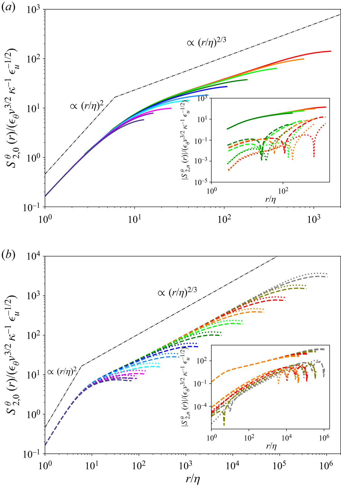
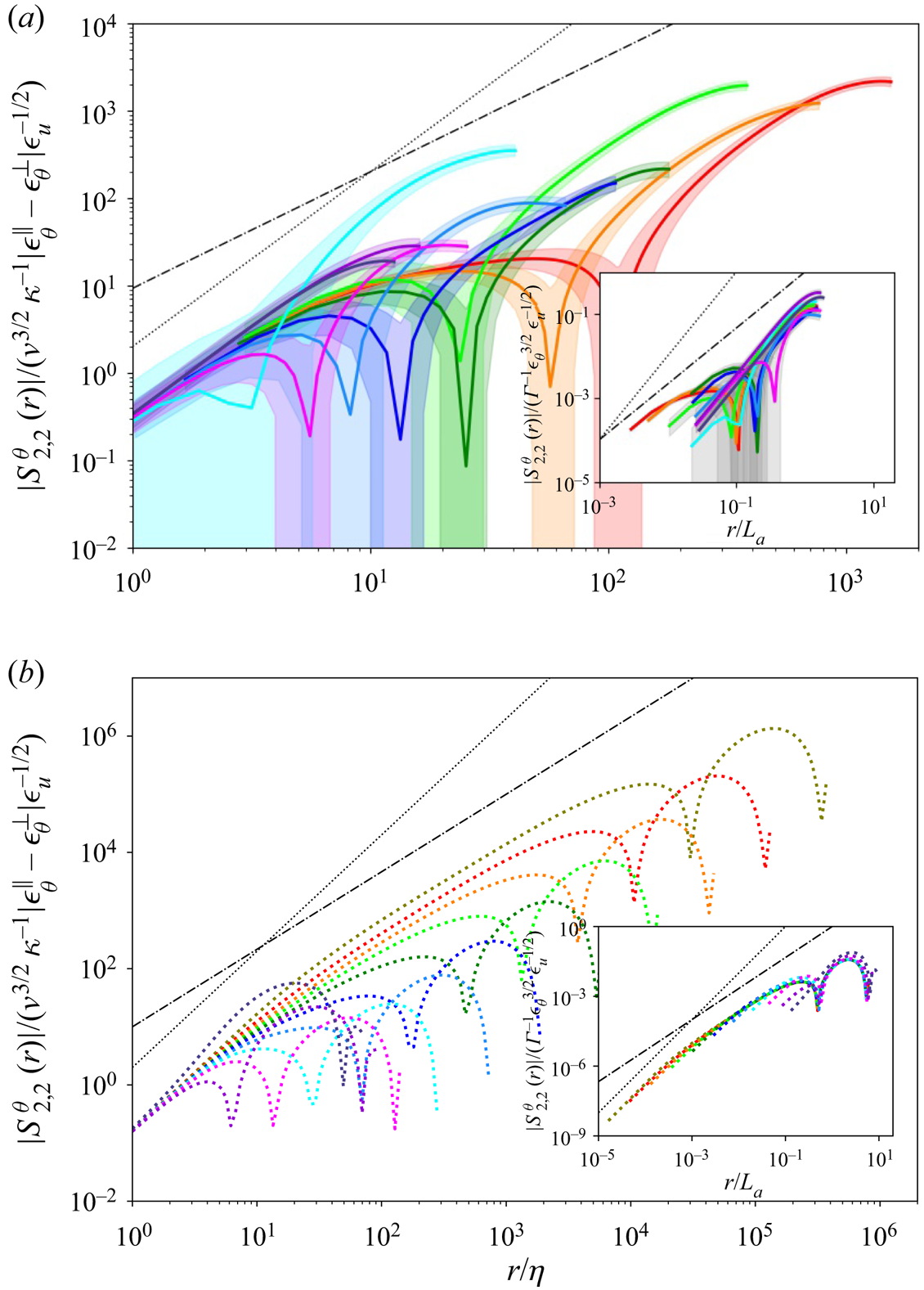
For the passive scalar fluctuation, we then computed the spherically averaged second-order structure function as follows:
 \begin{equation} S_{2,2n}^{\theta}\left(r\right)=2\sum_{\boldsymbol{k}}\hat{\theta}\left(\boldsymbol{k}\right)\hat{\theta}^{*} \left(\boldsymbol{k}\right)\left(4n+1\right)g_{2n}\left(kr\right)P_{2n}\left(\mu_{k}\right), \end{equation}
where  $g_{2n}(kr)$ is related to the spherical Bessel function, and
 $P_{2n}(\mu _{k})$ is the Legendre function. More details on the expressions for
 $g_{2n}$ and
 $P_{2n}$ are provided in § 4. This structure function was used for the extraction of isotropic and anisotropic components, and for the approximation of longitudinal- and transverse-order structure functions. The second-order structure function for the
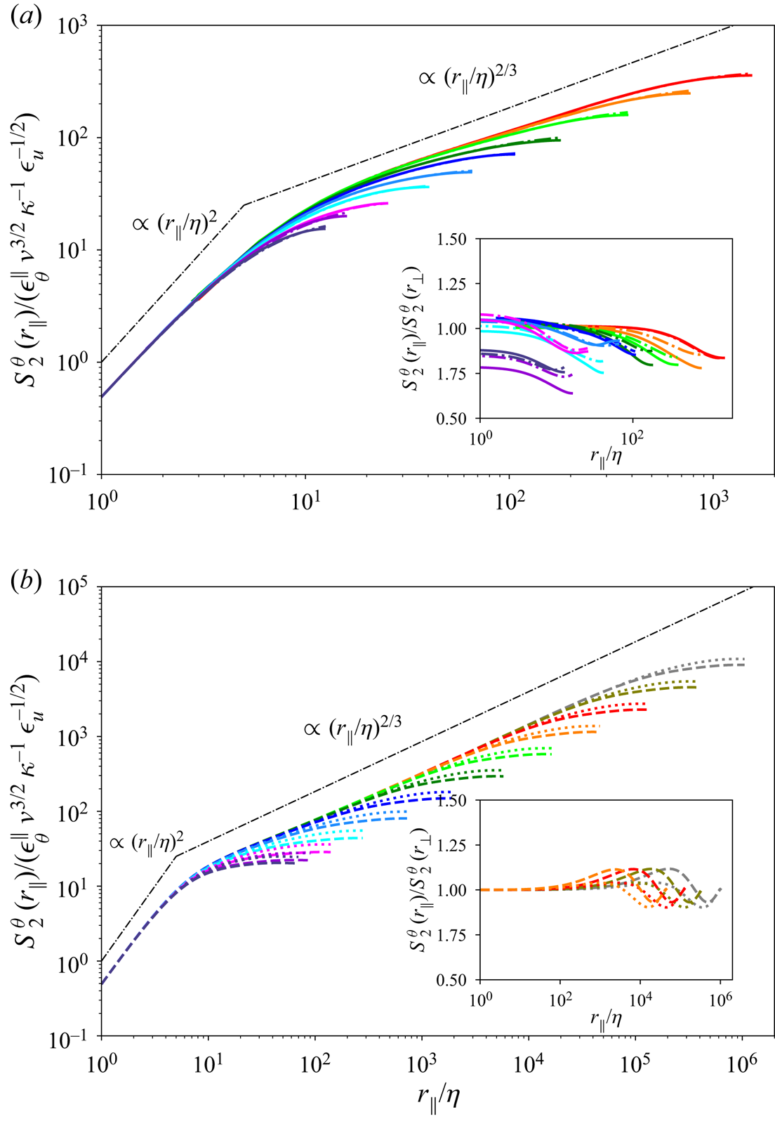
 $r_{m}$ direction was calculated as follows:
 \begin{equation} S_{2}^{\theta}\left(r_{m}\right)=2\sum_{\boldsymbol{k}}\hat{\theta} \left(\boldsymbol{k}\right)\hat{\theta}^{*}\left(\boldsymbol{k}\right)-2 \sum_{\substack{\boldsymbol{k}\\ \left({\neq} k_{m}\right)}} \left[\sum_{k_{m}} \hat{\theta}\left(\boldsymbol{k}\right)\hat{\theta}^{*}\left(\boldsymbol{k}\right)\exp \left(\imath k_{m}r_{m}\right)\right], \end{equation}
where  $\sum _{\boldsymbol {k}\\ (\neq k_{m})}$ signifies that the summation was obtained in two directions, i.e. excluding
 $k_{m}$, whereas the bracket part was calculated via the one-dimensional fast Fourier transform. Here,
 $S_{2}^{\theta }(r_{3})$ is the direct evaluation of the longitudinal second-order structure function;
 $S_{2}^{\theta }(r_{1})$ and
 $S_{2}^{\theta }(r_{2})$ are those of the transverse function.
4. Results and discussion
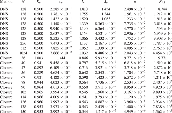
The velocity characteristics are summarised in table 1. Here  $K_{u}$,
 $\epsilon _{u}$,
 $L_{u}$,
 $\lambda _{u}$ and
 $\eta$ are the TKE, TKE dissipation rate, integral length scale, Taylor microscale and Kolmogorov scale, respectively. These are defined as
 $K_{u}=\int _{0}^{\infty }{\textrm {d}}k\, E_{u}(k)$,
 $\epsilon _{u}=2\nu \int _{0}^{\infty }{\textrm {d}}k\, k^{2}E_{u}(k)$,
 $L_{u}=3{\rm \pi} /(4K_{u})\int _{0}^{\infty }{\textrm {d}}k\, E(k)/k$,
 $\lambda _{u}^{2}=10\nu K_{u}/\epsilon _{u}$ and
 $\eta =(\nu ^{3}/\epsilon _{u})^{{1}/{4}}$, respectively. Here
 $Re_{\lambda }\equiv \sqrt {2K_{u}/3}\lambda _{u}/\nu$ is the turbulence Reynolds number based on the Taylor microscale. The characteristics of the velocity field are almost the same as in previous studies (Kitamura Reference Kitamura2020, Reference Kitamura2021), and thus the results on the velocity field are omitted in this paper (refer to our previous studies for details on velocity statistics).
Velocity characteristics in numerical simulations.

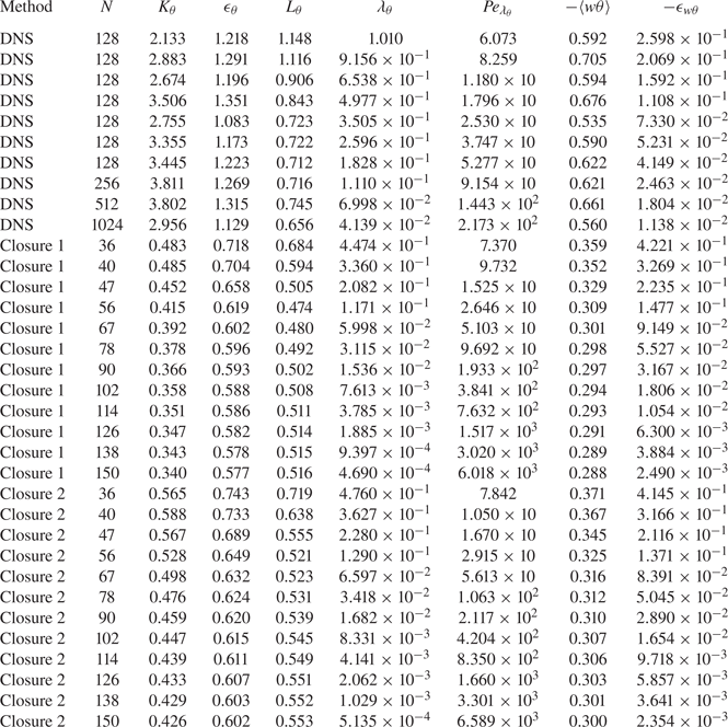
The scalar characteristics are summarised in table 2. Here  $K_{\theta }$,
 $\epsilon _{\theta }$,
 $L_{\theta }$,
 $\lambda _{\theta }$,
 $\langle w\theta \rangle$ and
 $\epsilon _{w\theta }$ are the scalar variance, scalar dissipation rate, scalar integral length scale, scalar Taylor microscale, scalar flux and scalar flux dissipation rate, respectively. These are defined as
 $K_{\theta }=\int _{0}^{\infty }{\textrm {d}}k\, E_{\theta }(k)$,
 $\epsilon _{\theta }=2\kappa \int _{0}^{\infty }{\textrm {d}}k\, k^{2}E_{\theta }(k)$,
 $L_{\theta }={\rm \pi} /(2K_{\theta })\int _{0}^{\infty }{\textrm {d}}k\, E_{\theta }(k)/k$,
 $\lambda _{\theta }^{2}=6\kappa \epsilon _{\theta }/K_{\theta }$,
 $\langle u_{3}\theta \rangle =\int _{0}^{\infty }{\textrm {d}}k\, F_{3}(k)$ and
 $\epsilon _{w\theta } =(\nu +\kappa )\int _{0}^{\infty }{\textrm {d}}k\, k^{2}F_{3}(k)$, respectively. Here
 $Pe_{\lambda _{\theta }}\equiv \sqrt {2K_{u}/3}\lambda _{\theta }/\kappa$ is the turbulence Péclet number based on the scalar Taylor microscale.
Scalar characteristics in numerical simulations, where velocity characteristics of closures 1 and 2 are the same. In figures for two-point statistics, the dashed and dotted lines are used in closures 1 and 2, respectively.

The integral length scale for the  $l$ direction is defined as the integral of the autocorrelation coefficient,
 \begin{equation} L_{\theta}^{\left(l\right)}=\frac{1}{\left\langle \theta^{2} \left(\boldsymbol{x}\right)\right\rangle}\int_{0}^{\infty}{\textrm{d}}r \left\langle \theta\left(\boldsymbol{x}\right)\theta\left(\boldsymbol{x}+r\boldsymbol{e}_{l}\right)\right\rangle = \frac{\rm \pi}{\left\langle \theta^{2}\left(\boldsymbol{x}\right)\right\rangle}\int {\textrm{d}}^{2}\boldsymbol{k} \varTheta\left(\boldsymbol{k}\right)|_{k_{l}=0}, \end{equation}
where the latter expression is valid for homogeneous turbulence (Cambon & Jacquin Reference Cambon and Jacquin1989). As discussed later, the autocorrelation coefficient can be expanded by Legendre polynomials because of the axisymmetry of the passive-scalar field. When the axisymmetry of the passive-scalar field is used, and the autocorrelation coefficient is integrated, the integral length scale is determined to be
 \begin{equation} L_{\theta}\left(\mu_{r}\right)=\frac{\sqrt{\rm \pi}}{\int_{0}^{\infty}{\textrm{d}}k\, E_{0}^{\left(\theta\right)}\left(k\right)}\int_{0}^{\infty}{\textrm{d}}k \sum_{n=0}^{\infty}\frac{E_{2n}^{\left(\theta\right)}\left(k\right)}{k}\left({-}1\right)^{n} \frac{\varGamma\left(n+\dfrac{1}{2}\right)}{2n!}P_{2n}\left(\mu_{r}\right), \end{equation}
where  $\varGamma (x)$ is the Gamma function. When the properties
 $P_{2n}(\mu _{r}=1)=1$ and
 $P_{2n}(\mu _{r}=0)=(-1)^{n}(2n)!/[2^{2n}(n!)^{2}]$ are used, the longitudinal and transverse integral length scales are calculated as
 $$\begin{gather} L_{\theta}^{{\parallel}}=L_{\theta}\left(\mu_{r}=1\right)=\frac{\sqrt{\rm \pi}}{\int_{0}^{\infty}{\textrm{d}}k\, E_{0}^{\left(\theta\right)}\left(k\right)}\int_{0}^{\infty}{\textrm{d}}k \sum_{n=0}^{\infty}\frac{E_{2n}^{\left(\theta\right)}\left(k\right)}{k}\left({-}1\right)^{n} \frac{\varGamma\left(n+\dfrac{1}{2}\right)}{2n!}, \end{gather}$$
 $$\begin{gather}L_{\theta}^{{\perp}}=L_{\theta}\left(\mu_{r}=0\right)=\frac{\sqrt{\rm \pi}}{\int_{0}^{\infty}{\textrm{d}}k\, E_{0}^{\left(\theta\right)}\left(k\right)}\int_{0}^{\infty}{\textrm{d}}k \sum_{n=0}^{\infty}\frac{E_{2n}^{\left(\theta\right)}\left(k\right)}{k} \frac{\varGamma\left(n+\dfrac{1}{2}\right)\left(2n\right)!}{2^{2n+1}\left(n!\right)^{3}}, \end{gather}$$
where  $L_{\theta }^{\parallel }$ and
 $L_{\theta }^{\perp }$ are, ideally, equivalent to
 $L_{\theta }^{(3)}$ and
 $(L_{\theta }^{(1)}+L_{\theta }^{(2)})/2$, respectively. In the closure, the longitudinal and transverse integral length scales are evaluated based on the second-order truncations in (4.3a) and (4.3b). The longitudinal and transverse scalar dissipation rates are defined as
 $\epsilon _{\theta }^{\parallel }=2\kappa \int {\textrm {d}}\boldsymbol {k}\, k_{3}^{2}\varTheta (\boldsymbol {k})$ and
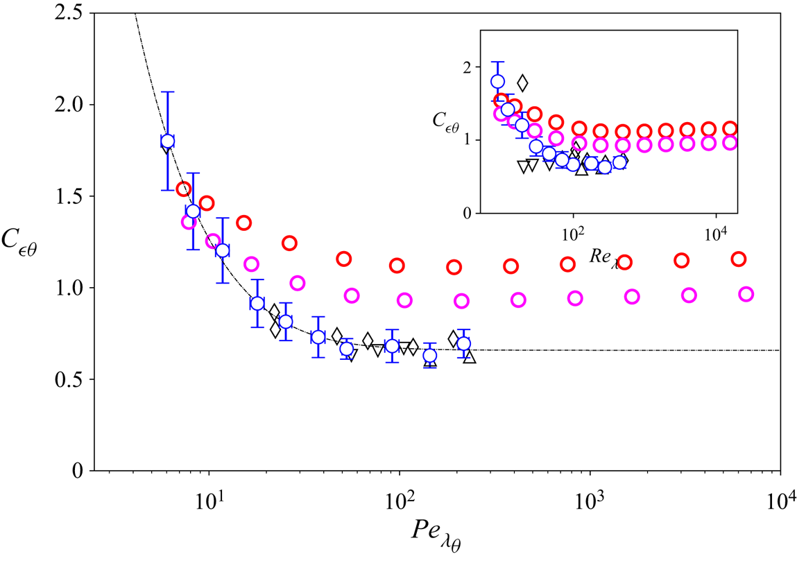
 $\epsilon _{\theta }^{\perp }=\kappa \int {\textrm {d}}\boldsymbol {k}\, (k_{1}^{2}+k_{2}^{2})\varTheta (\boldsymbol {k})$, respectively. Definitions of some of the statistical quantities used in closure are summarised in Appendix D. Figure 1 shows the relation between the normalised scalar dissipation rate
 $C_{\epsilon _{\theta }}\equiv \epsilon _{\theta }L_{u}/(K_{\theta }\sqrt {2/3K_{u}})$ and
 $Pe_{\lambda _{\theta }}$ obtained based on closures and DNS together with DNS data from previous studies. The inset shows the relation between
 $C_{\epsilon _{\theta }}$ and
 $Re_{\lambda }$, where the Péclet number based on the velocity Taylor microscale obeys
 $Pe_{\lambda _{u}}=Re_{\lambda }$ because
 $Sc=1$, therefore, we use
 $Re_{\lambda }$ instead of
 $Pe_{\lambda _{u}}$ hereafter. Although there is a rigorous mathematical proof of the bounds on the energy dissipation rate (Doering & Foias Reference Doering and Foias2002), no similar general result is known for those on the scalar dissipation rate. It may be natural to assume that both have the same functional form:
 \begin{equation} C_{\epsilon_{\theta}}=a\left[1+\sqrt{1+\left(\frac{b}{Pe_{\lambda_{\theta}}}\right)^{2}}\right]. \end{equation}
This expression can be compared with an alternative functional form, applied in previous studies, that uses  $Re_{\lambda }$ (Donzis et al. Reference Donzis, Sreenivasan and Yeung2005). As shown in Figure 1, the use of
 $Pe_{\lambda _{\theta }}$, rather than
 $Re_{\lambda }$, seems to result in a better collapse of
 $C_{\epsilon _{\theta }}$. Similar findings for other passive-scalar statistics have also been recently reported by Yasuda et al. (Reference Yasuda, Gotoh, Watanabe and Saito2020). Direct numerical simulation and closure results show that the scalar dissipation rate is independent of
 $\kappa$ for high
 $Pe_{\lambda _{\theta }}$, but its asymptotic value at high
 $Pe_{\lambda _{\theta }}$ is quantitatively different; the second closure is better in that quantitative sense. Nevertheless, both closures are qualitatively valid in a wide range of
 $Pe_{\lambda _{\theta }}$.
Normalised scalar dissipation rate  $C_{\epsilon _{\theta }}$ versus Péclet number
 $Pe_{\lambda _{\theta }}$ with
 $\pm \sigma$ error bars for present DNSs, where
 $\sigma$ is the standard deviation. Also included are DNS data from Donzis, Sreenivasan & Yeung (Reference Donzis, Sreenivasan and Yeung2005) and references therein for unity Schmidt number. Red, magenta and blue circles represent closure 1, closure 2 and DNS results, respectively. Black diamond, upward triangle and downward triangles denote results from Donzis et al. (Reference Donzis, Sreenivasan and Yeung2005), Watanabe & Gotoh (Reference Watanabe and Gotoh2004) and Wang, Chen & Brasseur (Reference Wang, Chen and Brasseur1999), respectively. Insets shows
 $C_{\epsilon _{\theta }}$ versus Reynolds number
 $Re_{\lambda }$.

As in EDNQM (Cambon et al. Reference Cambon, Jeandel and Mathieu1981; Bos et al. Reference Bos, Touli and Bertoglio2005), involving the linear term (the mean scalar gradient in this study) in the triad interaction makes the accuracy of the model worse. This finding will contribute to a further development of spectral modelling when one applies the DIA families to the single-time two-point closure.
On the other hand, the DNS results in this study are in good agreement with the results of previous studies (Donzis et al. Reference Donzis, Sreenivasan and Yeung2005). Because of the quantitative difference between the results for DNS and closure, parameter fitting was performed only for the DNS results and was evaluated by the Levenberg–Marquardt least-squares method. The results show that  $a=0.329$ and
 $b=26.66$, so that this study predicts that
 $C_{\epsilon _{\theta }}$ approaches 0.65 as
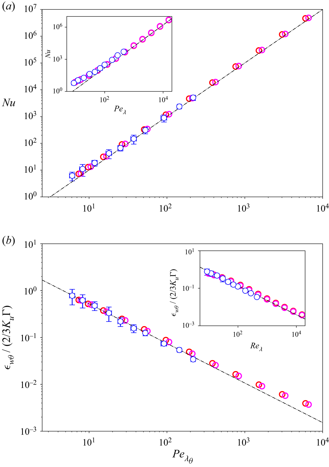
 $Pe_{\lambda _{\theta }}\to \infty$. Figure 2(a) shows the dependence of the Nusselt number
 $Nu=-\langle w\theta \rangle /(\kappa \varGamma )$ on
 $Pe_{\lambda _{\theta }}$, whereas the inset shows the corresponding dependence on
 $Re_{\lambda }$. As discussed in Gotoh & Watanabe (Reference Gotoh and Watanabe2012),
 $Nu\propto Pe_{L}\sim Re_{\lambda }^{2}$, where
 $Pe_{L}=\sqrt {2/3K_{u}}L_{u}/\kappa$, and therefore
 $Nu\propto Pe_{\lambda _{\theta }}$ because
 $\lambda _{\theta }/\lambda _{u}$ approaches a constant value at high
 $Pe_{\lambda _{\theta }}$. Unlike the best-fit power law for
 $Re_{\lambda }$, the best-fit power law
 $Nu=a_{Nu}Pe_{\lambda _{\theta }}^{2}$ properly collapses for the DNS and closure results, where
 $a_{Nu}=0.1$. The least-squares method was applied only on the closure results because of the good agreement between DNS and closure.
The  $Pe_{\lambda _{\theta }}$ dependences of (a) Nusselt number and (b) ratio of
 $\epsilon _{w\theta }$ and
 $2/3\varGamma K_{u}$. Insets show corresponding
 $Re_{\lambda }$ dependences. Dash–dot lines visualise best-fit power laws. For symbol legends, refer to the caption in figure 1.

The present scaling is useful for the qualitative evaluation of mixing. However, the other scaling  $Nu\propto Pe_{L}^{0.55}$ has been also reported in an experiment (Mydlarski & Warhaft Reference Mydlarski and Warhaft1998). The reason for this is not known, and it would be interesting to validate the present scaling on
 $Sc$ in the future study.
Figure 2(b) shows the dependence of the ratio of the scalar flux dissipation  $-\epsilon _{w\theta }$ and scalar flux production
 $2/3\varGamma K_{u}$ on
 $Pe_{\lambda _{\theta }}$, whereas the inset shows the corresponding dependence on
 $Re_{\lambda }$. The dash–dot line in figure 2(b) shows
 $4.61Re_{\lambda }^{-0.769}$, which was observed in previous DNSs by Overholt & Pope (Reference Overholt and Pope1996) and EDQNM (Bos et al. Reference Bos, Touli and Bertoglio2005). The dash–dot line in the inset of figure 2(b) shows the best-fitting power law, which is of the form
 $-\epsilon _{w\theta }/(2/3\varGamma K_{u})=a_{\epsilon _{w\theta }}Pe_{\lambda _{\theta }}^{-b_{\epsilon _{w\theta }}}$, where
 $a_{\epsilon _{w\theta }}=3.65$ and
 $b_{\epsilon _{w\theta }}=0.84$. Here, fitting was performed only on the DNS results. A slight departure from the fitting curve can be observed at high
 $Pe_{\lambda _{\theta }}$ regimes. Furthermore, clear
 $Re_{\lambda }^{-1}$ scaling is not observed for high Reynolds number regimes, i.e.
 $Re_{\lambda }\ge O(10^{3})$; this differs from the results of analyses and numerical methods on EDQNM (Bos et al. Reference Bos, Touli and Bertoglio2005; Briard et al. Reference Briard, Gomez, Sagaut and Memari2015). As discussed later, this may be related to the dependence of the cospectral bump on
 $Pe_{\lambda _{\theta }}$. There is also a quantitative difference between the EDQNM results in Bos et al. (Reference Bos, Touli and Bertoglio2005) and those in Briard et al. (Reference Briard, Gomez, Sagaut and Memari2015), although
 $Re_{\lambda }$ scaling is applicable to both. Thus, whether
 $-\epsilon _{w\theta }/(2/3\varGamma K_{u})\propto Re_{\lambda }^{-1}$ remains valid is an open question within the framework of closure theories and may require high
 $Pe_{\lambda _{\theta }}$ DNSs or experiments of order
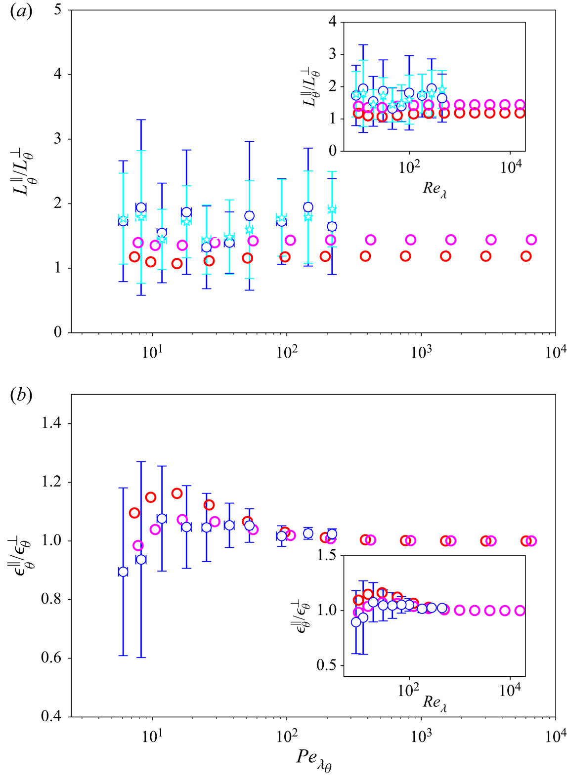
 $Pe_{\lambda _{\theta }}\sim O(10^{3})$ to be resolved. Figures 3(a) and 3(b) show the dependence of large- and small-scale anisotropies on
 $Pe_{\lambda _{\theta }}$. Large-scale anisotropies, in contrast to small-scale ones, are characterised by conspicuous unsteadiness, as visualised by the error bars. In figure 3(a), the different evaluations of large-scale anisotropy are shown. We have confirmed the quantitative agreement between (4.1) and (4.2) by monitoring the temporal evolutions of
 $L_{\theta }^{\parallel }$ and
 $L_{\theta }^{\perp }$ in DNS. Both closure results are quantitatively in agreement within the acceptable
 $\pm$ range of standard deviations around DNS data, although closure 2 yields better results than does closure 1. As shown in figure 3(a), large-scale anisotropies persist regardless of
 $Pe_{\lambda _{\theta }}$. On the other hand, small-scale anisotropies are below unity when
 $Pe_{\lambda _{\theta }}\le 20$, reach a maximum at
 $Pe_{\lambda _{\theta }}\sim 20$ and approach unity as
 $Pe_{\lambda _{\theta }}\to \infty$. Thus, the effect of turbulent mixing becomes more significant as
 $Pe_{\lambda _{\theta }}$ increases. Consequently, the results are consistent with the local isotropy theory within the framework of evaluation of second-order moments. Similar tendencies in small-scale anisotropies were noted by Yasuda et al. (Reference Yasuda, Gotoh, Watanabe and Saito2020) for the low
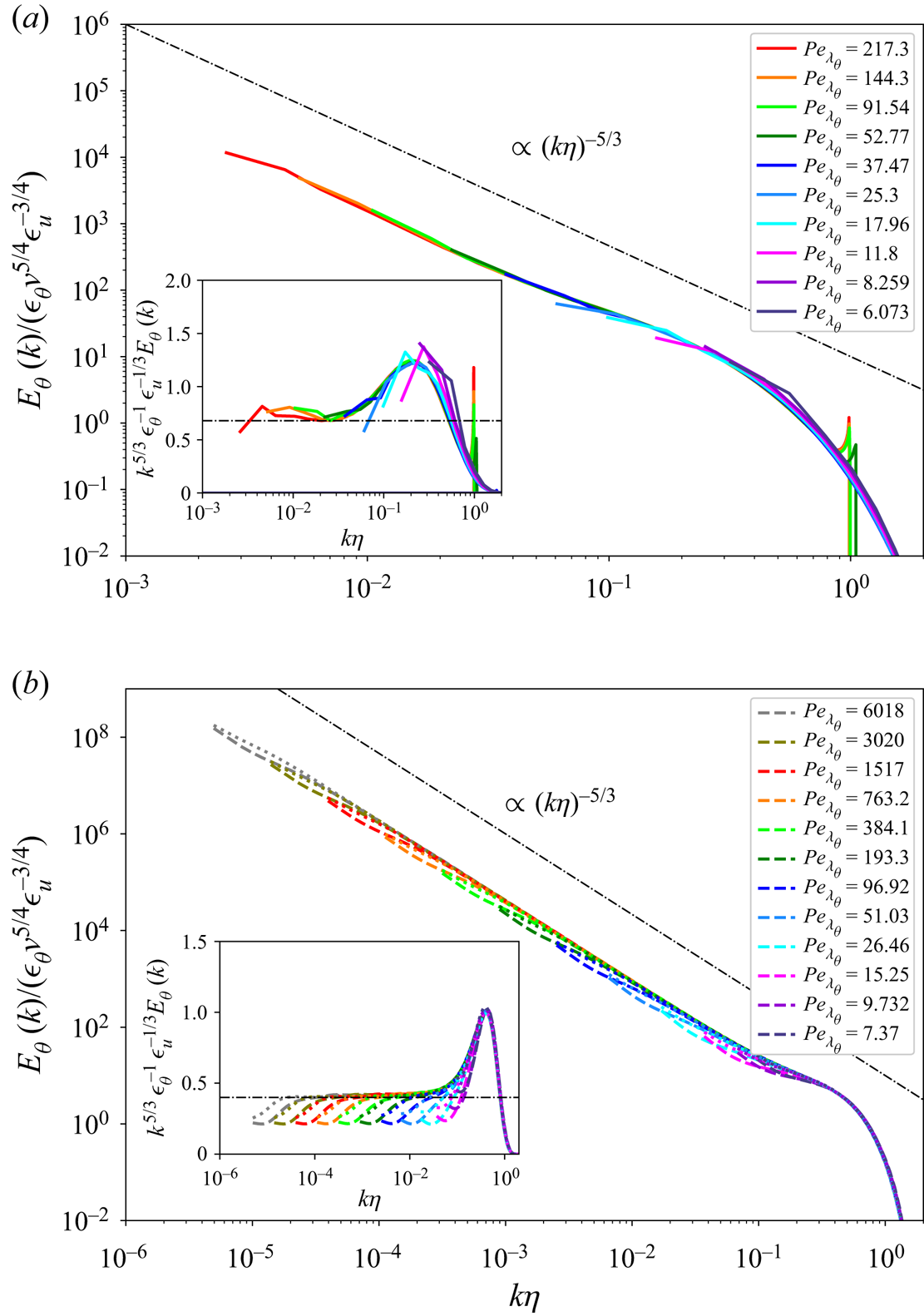
 $Pe_{\lambda _{\theta }}$ regimes. When Kolmogorov–Obukhov–Corrsin phenomenology is applicable, the scalar spectrum in the universal equilibrium range behaves as
 \begin{equation} E_{\theta}\left(k\right)=\epsilon_{\theta}\nu^{{5}/{4}}\epsilon_{u}^{-({3}/{4})} \tilde{E}_{\theta}\left(k\eta\right). \end{equation}
In the inertial convective range this becomes  $E_{\theta }=\tilde {K}_{\theta }\epsilon _{\theta }\epsilon _{u}^{-({1}/{3})}k^{-({5}/{3})}$, where the scaling is independent of
 $\nu$ and
 $\kappa$. Figure 4 shows the normalised scalar spectra, whereas the insets show the compensated scalar spectra. As shown in figure 4, the scalar spectra collapse properly with the increase in
 $Pe_{\lambda _{\theta }}$ in the inertial convective and dissipation ranges for both DNS and closures, despite the quantitative difference between DNS and closure results. Compared with those in the energy spectra (Donzis & Sreenivasan Reference Donzis and Sreenivasan2010; Kitamura Reference Kitamura2020), the heights of bumps in the scalar spectra seem to be independent of
 $Pe_{\lambda _{\theta }}$, and the manifestation of the
 $-5/3$ law in the scalar spectra seems to be faster; it is necessary that
 $Re_{\lambda }\sim O(10^{4})$ for the
 $-5/3$ law of energy spectra to manifest in closure theory. The difference between closures 1 and 2 is observed mainly in the lowest wavenumber range; it is negligible in the inertial convective and dissipation ranges.
The  $Pe_{\lambda _{\theta }}$ dependence of (a) large- and (b) small-scale anisotropies. Insets show corresponding
 $Re_{\lambda }$ dependence. Here, blue circles and cyan stars in panel (a) represent DNS results estimated using (4.1) and second-order truncation of (4.2), respectively. For other symbol legends, refer to the caption in figure 1.

Normalised scalar spectra for (a) DNS and (b) closures. Insets show compensated scalar spectra, where black dash–dot lines show  $\tilde {K}_{\theta }=0.68$ in panel (a) and
 $\tilde {K}_{\theta }=0.4$ in panel (b). Dashed and dotted lines in panel (b) signify closures 1 and 2, respectively. Here, legends for closure 2 are omitted; detailed information is in table 2.

The quantitative difference between DNS and closures is the Obukhov–Corrsin constant,  $\tilde {K}_{\theta }$. Other closure theories that do not involve any introduction of adjustable parameters also exhibit a lower value of
 $\tilde {K}_{\theta }$, e.g.
 $\tilde {K}_{\theta }=0.34$ for homogeneous isotropic passive scalar in LDIA (Goto & Kida Reference Goto and Kida1999) and
 $\tilde {K}_{\theta }=0.208$ for homogeneous isotropic passive scalar in abridged Lagrangian history DIA (Kraichnan Reference Kraichnan1966). The lower estimate of
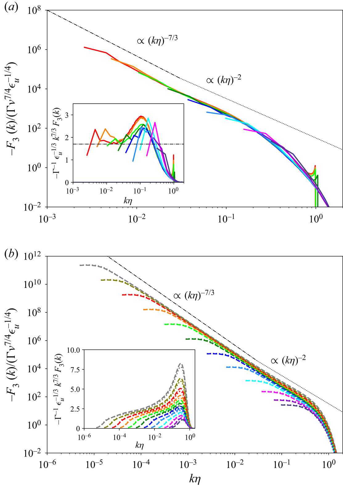
 $\tilde {K}_{\theta }$ in the closures is one of the reasons for the quantitative differences in the scalar statistics shown in figure 1. Based on Lumley (Reference Lumley1964, Reference Lumley1967), the velocity–scalar cospectrum in the universal equilibrium range obeys
 \begin{equation} F_{3}\left(k\right)=\varGamma\nu^{{7}/{4}}\epsilon_{u}^{-({1}/{4})}\tilde{F}_{3}\left(k\eta\right), \end{equation}
which results in the inertial convective range  $F_{3}(k)=\tilde {K}_{w\theta }\varGamma \epsilon ^{{1}/{3}}k^{-({7}/{3})}$. Figure 5 shows the normalised cospectra, whereas the insets show the compensated cospectra. The difference between closures 1 and 2 is negligible, and only a slight difference is observed at the bump regime. As shown in figures 5(a) and 5(b), the coexistence of
 $-7/3$ and
 $-2$ laws is observed as in Gotoh & Watanabe (Reference Gotoh and Watanabe2012). Although the clear
 $-7/3$ law regime is not observed in the present closures even for high
 $Re_{\lambda }$, this is related to the
 $Re_{\lambda }$ dependence of cospectral slope. As demonstrated for EDQNM (Bos et al. Reference Bos, Touli and Bertoglio2005), the
 $-7/3$ law is achieved only at very high
 $Re_{\lambda }\sim O(10^{7})$, but, in this study,
 $Re_{\lambda }\sim O(10^{4})$. The results of the present closure in the inertial convective range are qualitatively consistent with those of EDQNM (Bos et al. Reference Bos, Touli and Bertoglio2005). In fact, the cospectral slope in this regime is steeper than
 $-2$ for higher
 $Re_{\lambda }$, but close to
 $-2$ for lower. Thus, the cospectral slope is a function of
 $Re_{\lambda }$, and Lumley's
 $-7/3$ law would be achieved only at the higher
 $Re_{\lambda }$. This does not contradict experiment (Mydlarski & Warhaft Reference Mydlarski and Warhaft1998) or EDQNM (Bos et al. Reference Bos, Touli and Bertoglio2005). Thence, the theoretical estimation by present closure at the inertial subrange is a reasonable result.
Normalised velocity–scalar cospectra for (a) DNS and (b) closures. The dash–dot and dotted lines represent  $-$7/3 and
 $-$2 slopes, respectively. Insets show compensated cospectra; the black dash–dot line in panel (a) represents
 $K_{w\theta }=1.7$. For legends, refer to table 2 and figure 4.

With both DNS and closures, the cospectral bump monotonically increases with the increase in  $Pe_{\lambda _{\theta }}$, whereas that of the scalar spectrum may be independent of
 $Pe_{\lambda _{\theta }}$, and that of the energy spectrum may decrease with the increase in
 $Re_{\lambda }$. The heights of cospectral bumps in closures 1 and 2 are larger than EDQNM results reported in Bos et al. (Reference Bos, Touli and Bertoglio2005). More specifically, the clear
 $Pe_{\lambda _{\theta }}$-dependence of the height was not observed in EDQNM.
Thus, the main difference between the present closures and EDQNM is in the prediction of the cospectral bump. The departure from  $\epsilon _{w\theta }/(2/3\varGamma K_{u})\sim Pe_{\lambda _{\theta }}^{-1}$ scaling at higher
 $Pe_{\lambda _{\theta }}$ regimes comes mainly from the
 $Pe_{\lambda _{\theta }}$ dependence of the cospectral bump, which should be investigated further, via high
 $Pe_{{\lambda }_{\theta }}$ DNSs or experiments, to determine whether
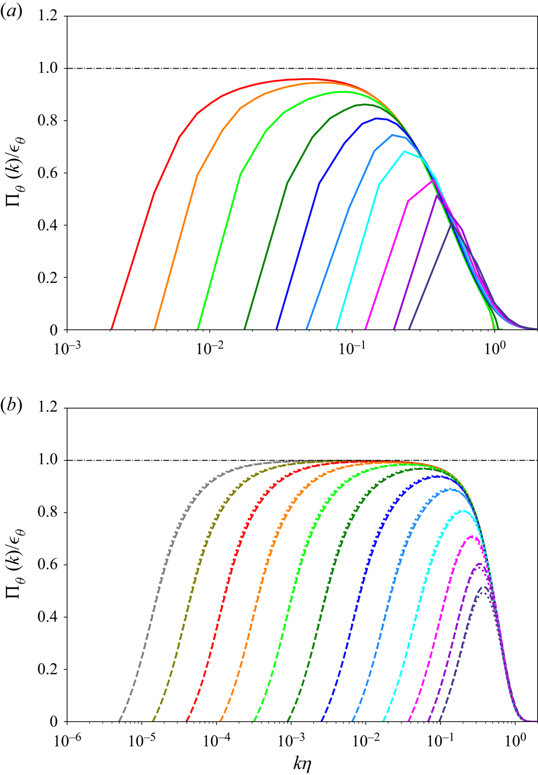
 $\epsilon _{w\theta }/(2/3\varGamma K_{u})\propto Pe_{\lambda _{\theta }}^{-1}$. The scalar transfer flux is defined as
 $\varPi _{\theta }(k)=\int _{k}^{\infty }{\textrm {d}}p\, T_{\theta }(p)=-\int _{0}^{k}{\textrm {d}}p\, T_{\theta }(p)$, where
 $T_{\theta }(k)$ is the scalar transfer function. For a high-Péclet-number passive-scalar field,
 $\varPi _{\theta }(k)=\epsilon _{\theta }$ is satisfied in the same way that
 $\varPi _{u}(k)=\epsilon _{u}$ is satisfied for a velocity field in high-Reynolds-number turbulent flow, where
 $\varPi _{u}(k)$ is the energy flux. Figures 6(a) and 6(b) show the normalised scalar transfer fluxes for DNSs and closures, respectively. Note that
 $\varPi _{\theta }(k)$ approaches
 $\epsilon _{\theta }$ with the increase in
 $Pe_{\lambda _{\theta }}$, and that the differences in results between the DNSs and closures are negligible.
Normalised scalar transfer fluxes for (a) DNS and (b) closures. Horizontal straight dash–dot lines show unity.

With both the DNSs and closures, the approach to  $\varPi _{\theta }(k)=\epsilon _{\theta }$ is slower than that to
 $\varPi _{u}(k)=\epsilon _{u}$, despite the approach to the
 $-5/3$ law of scalar spectra being faster than that of energy spectra (refer to Kitamura (Reference Kitamura2020) for details on energy spectra and fluxes). This slow approach of
 $\varPi _{\theta }(k)$ to
 $\epsilon _{\theta }$ can be understood from the scale-by-scale budget. Using (2.13a) and (2.13c), and assuming the statistically steady state, we have
 $\varPi _{u}(k)=\int _{k}^{\infty }{\textrm {d}}p\, 2\nu k^{2}E_{u}(p)-\int _{k}^{\infty }{\textrm {d}}p\, E_{f}(p)$ and
 $\varPi _{\theta }(k)=\int _{k}^{\infty }{\textrm {d}}p\, 2\kappa p^{2}E_{\theta }(p)+4/3\varGamma \int _{k}^{\infty }{\textrm {d}}p\, F(p)$. We can, therefore, estimate
 $\varPi _{u}(k)\sim \epsilon _{u}$ in the inertial subrange and
 $\varPi _{\theta }(k)\sim \epsilon _{\theta }+4/3\varGamma \int _{k}^{\infty }{\textrm {d}}p\, F(p)$ in the inertial convective range, where we assume that the effect of low-wavenumber forcing is neglected. That of velocity–scalar cospectra, however, cannot be neglected in the inertial convective range, as shown in figure 5. Thus, the approach of
 $\varPi _{\theta }(k)$ to
 $\epsilon _{\theta }$ is slower than that of
 $\varPi _{u}(k)=\epsilon _{u}$, and the fast approach of
 $\varPi _{\theta }(k)$ to
 $\epsilon _{\theta }$ would also be observed for a passive scalar sustained by random forcing at low wavenumbers.
Furthermore, it is expected from the analogy with the velocity field that the approach to Yaglom's  $4/3$ law in the passive scalar with a mean scalar gradient should also be slower than that in the passive scalar sustained by random forcing at low wavenumbers. However, the
 $Pe_{\lambda _{\theta }}$ dependence and effect of forcing are unclear, and the approach to the
 $4/3$ law remains an interesting topic for future study.
On the other hand, it is intriguing to observe a clear  $-5/3$ law for the passive scalar. The appearance of a
 $-5/3$ law in the scalar spectrum at low
 $Re_{\lambda }$ has been also observed in grid-turbulence experiments despite the absence of Kolmogorov scaling in the velocity field (Warhaft Reference Warhaft2000). These results may imply that the formation of a
 $-5/3$ law of the scalar spectrum is not described by the cascade picture of Kolmogorov (Reference Kolmogorov1941a,Reference Kolmogorovb), Obukhov (Reference Obukhov1949) and Corrsin (Reference Corrsin1951). However, it is not clear why this should be so, and further investigation is necessary. The second-order scalar structure function is defined as
 \begin{align} S_{2}^{\theta}\left(\boldsymbol{r}\right)&=\left\langle \left(\theta\left(\boldsymbol{x}+\boldsymbol{r}\right)-\theta\left(\boldsymbol{x}\right)\right)^{2}\right\rangle=2 \int {\textrm{d}}\boldsymbol{k}\, \varTheta\left(\boldsymbol{k}\right)\left[1-\exp\left(\imath\boldsymbol{k}\cdot\boldsymbol{r}\right)\right] \nonumber\\ &=2\int {\textrm{d}}\boldsymbol{k}\, \varTheta\left(\boldsymbol{k}\right)\left[1-4{\rm \pi}\sum_{l=0}^{\infty} \sum_{m={-}l}^{l}\imath^{l}j_{l}\left(kr\right)Y_{l}^{m}\left(\boldsymbol{k}\right)Y_{l}^{m*} \left(\boldsymbol{r}\right)\right], \end{align}
where the second expression is derived using the plane wave expansion and the spherical harmonic addition theorem (Arfken & Weber Reference Arfken and Weber1999; Gotoh et al. Reference Gotoh, Watanabe and Suzuki2011). Here,  $j_{l}$ and
 $Y_{l}^{m}$ are the spherical Bessel function and spherical harmonic function, respectively. The integration in the azimuthal direction causes the terms containing spherical harmonics to vanish when
 $m\neq 0$ if the passive-scalar field is axisymmetric. When axisymmetry is assumed, the second-order scalar structure function may be expressed as
 \begin{align} S_{2}^{\theta}\left(\boldsymbol{r}\right)&=4{\rm \pi}\int_{0}^{\infty}{\textrm{d}}k \int_{{-}1}^{1}{\textrm{d}}\mu_{k}\, k^{2}\varTheta\left(k,\mu_{k}\right) \nonumber\\ &\quad \times\left[1-\sum_{n=0}^{\infty}\left({-}1\right)^{n}\left(4n+1\right)j_{2n} \left(kr\right)P_{2n}\left(\mu_{k}\right)P_{2n}\left(\mu_{r}\right)\right] \nonumber\\ &=S_{2,0}^{\theta}\left(r\right)-\sum_{n=1}^{\infty}\left({-}1\right)^{n}S_{2,2n}^{\theta} \left(r\right)P_{2n}\left(\mu_{r}\right), \end{align}
where  $\mu _{r}$ is the cosine of the polar angle in physical space, defined as
 $\mu _{r}=\boldsymbol {r}\cdot \boldsymbol {n}/r$. From the definition, the isotropic and anisotropic scalar structure functions are given as
 $$\begin{gather} S_{2,0}^{\theta}\left(r\right)=2\int {\textrm{d}}\boldsymbol{k}\, \varTheta\left(\boldsymbol{k}\right)\left[1-j_{0}\left(kr\right)\right], \end{gather}$$
 $$\begin{gather}S_{2,2n}^{\theta}\left(r\right)=2\int {\textrm{d}}\boldsymbol{k}\, \varTheta\left(\boldsymbol{k}\right)\left(4n+1\right)j_{2n}\left(kr\right)P_{2n}\left(\mu_{k}\right), \end{gather}$$
where  $g_{2n}(kr)$ in (3.5) is
 $g_{2n}(kr)=1-j_{0}(kr)$ for
 $n=0$, and
 $g_{2n}(kr)=j_{2n}(kr)$ for
 $n\neq 0$. Based on the Taylor expansion of the spherical Bessel function
 $j_{n}(x)=(2x)^{n}\sum _{m=0}^{\infty }({(-1)^{m}(n+m)!}/{m!(2n+2m+1)!})x^{2m}$,
 \begin{gather} S_{2,0}^{\theta}\left(r\to 0\right)=\frac{r^{2}}{3}\int {\textrm{d}}\boldsymbol{k}\, k^{2}\varTheta\left(\boldsymbol{k}\right)-\sum_{m=2}^{\infty} \frac{2\left({-}1\right)^{m}}{\left(2m+1\right)!}r^{2m} \int {\textrm{d}}\boldsymbol{k}\, k^{2m}\varTheta\left(\boldsymbol{k}\right) \nonumber\\ =\frac{\epsilon_{\theta}}{6\kappa }r^{2}+O\left(r^{4}\right), \end{gather}
 \begin{gather} S_{2,2n}^{\theta}\left(r\to 0\right)=2^{2n+1}r^{2n} \frac{\varGamma\left(2n+1\right)}{\varGamma\left(4n+1\right)} \int {\textrm{d}}\boldsymbol{k}\, k^{2n}P_{2n}\left(\mu_{k}\right) \varTheta\left(\boldsymbol{k}\right)+O\left(r^{2n+2}\right), \end{gather}
where contributions from  $n\ge 2$ are neglected in the closures. From (4.10a), the universal functional form, which corresponds to (4.5) in spectral space, may be expressed as
 \begin{equation} S_{2,0}^{\theta}\left(r\right)=\epsilon_{\theta}\nu^{{3}/{2}}\kappa^{{-}1}\epsilon_{u}^{-({1}/{2})} \tilde{S}_{2,0}^{\theta}\left(\frac{r}{\eta}\right), \end{equation}
which becomes in the inertial convective range  $S_{2,0}(r)=C_{\theta }\epsilon _{\theta }\epsilon _{u}^{-({1}/{3})}r^{{2}/{3}}$, where
 $C_{\theta }$ is the Obukhov–Corrsin constant. Alternative forms using the Obukhov–Corrsin length and Batchelor length are also valid.
Figure 7 shows the normalised second-order isotropic scalar structure functions  $\tilde {S}_{2,0}^{\theta }(r/\eta )$, which properly collapse according to (4.11). The inset in figure 7 shows the contribution of the degree of the Legendre polynomials. As in the previous study (Gotoh et al. Reference Gotoh, Watanabe and Suzuki2011),
 $|S_{2,n}^{\theta }(r)|$ with degrees
 $n=2$ and
 $n=4$ are observed to be smaller in magnitude by orders of approximately two and four, respectively, than the isotropic component
 $S_{2,0}^{\theta }(r)$. Thus, the DNS results guarantee that the second-order truncation of the Legendre polynomial is valid, at least in a practical sense; further quantitative assessment by DNS is discussed later. The inset in figure 7 also exhibits extrema for
 $|S_{2,2}^{\theta }(r)|$ and
 $|S_{2,4}^{\theta }(r)|$. These extrema indicate zero-crossing points in
 $S_{2,2}^{\theta }(r)$ and
 $S_{2,4}^{\theta }(r)$, i.e. the signs of
 $S_{2,2}^{\theta }(r)$ and
 $S_{2,4}^{\theta }(r)$ alter at each extremum. From (4.11),
 $S_{2,2}^{\theta }(r)$ is inferred to obey
 \begin{equation} S_{2,2}^{\theta}\left(r\to 0\right)=\frac{\epsilon_{\theta}^{{\parallel}}- \epsilon_{\theta}^{{\perp}}}{3\kappa}r^{2}+O\left(r^{4}\right), \end{equation}
which implies that the sign of  $S_{2,2}^{\theta }(r)$ at small scales depends only on
 $\epsilon _{\theta }^{\parallel }-\epsilon _{\theta }^{\perp }$.
Normalised second-order scalar structure functions for (a) DNS and (b) closures. Inset in panel (a) shows absolute values of scalar structure functions for  $n=0$ (solid lines),
 $n=2$ (dashed lines) and
 $n=4$ (dotted lines); results for only the four highest Péclet numbers are shown for simplicity. Inset in panel (b) shows the absolute values of scalar structure functions for
 $n=0$ and
 $n=2$; dashed and dotted lines are results for closures 1 and 2, respectively.

Except for the two lowest Péclet numbers,  $S_{2,2}^{\theta }(r)$ is determined through DNS to be positive at small scales and negative at large, whereas
 $S_{2,4}^{\theta }(r)$ is negative at small scales and positive at large. On the other hand, for the two lowest Péclet numbers,
 $S_{2,2}^{\theta }(r)$ is negative at all scales. These observations are in accordance with the results shown in figure 3, i.e.
 $S_{2,2}^{\theta }(r\to 0)$ is positive at small scales for high
 $Pe_{\lambda _{\theta }}$ and negative at small scales for low
 $Pe_{\lambda _{\theta }}$.
A similar conclusion with regard to the sign of  $S_{2,4}^{\theta }(r\to 0)$ will be also obtained based on the Taylor expansion of (4.10b) for
 $n=2$. These extrema and positive
 $S_{2,2}^{\theta }(r\to 0)$ are observed in both DNSs and closures, although the locations of the extrema are different between closures. The locations of the extrema for closure 2 are closer to those for DNS than are those for closure 1, although the qualitative differences are observed mainly at large scales. From the insets in figure 7(b), the anisotropic components
 $S_{2,n}^{\theta }(r)$ for
 $n=2$ and
 $n=4$ are clearly different from the scaling law given by (4.11). Previous studies have established little concerning the scaling laws of the anisotropic scalar structure function; based on (4.12), it may have the following universal functional form:
 \begin{equation} S_{2,2}^{\theta}\left(r\right)=\frac{1}{3}\frac{\nu^{{3}/{2}}}{\kappa} \frac{\epsilon_{\theta}^{{\parallel}}-\epsilon_{\theta}^{{\perp}}}{\sqrt{\epsilon_{u}}}\tilde{S}_{2,2}^{\theta} \left(\frac{r}{\eta}\right). \end{equation}
Figures 8(a) and 8(b) show the DNS and closure results of the normalised anisotropic scalar structure function defined by (4.13), where only the results of closure 2 are shown. It can be seen that the scaling law given by (4.13) qualitatively collapses at small scale.
Normalised anisotropic scalar structure function based on (4.13) for (a) DNS and (b) closure 2; the results for closure 1 are omitted because they are worse in a qualitative sense. The dash–dot and dotted lines show the slope of  $r^{{4}/{3}}$ and
 $r^{2}$, respectively. Inset shows the normalised anisotropic structure function (4.15). For DNS, error bars are shown by slightly transparent colours (grey colours are used for error bars in inset). The error bars show the 95 % confidence interval.

While a scaling law of the form (4.13) may be valid for the second-order anisotropic scalar structure function for low to moderate  $Pe_{\lambda _{\theta }}$, the present scaling is not applicable for higher
 $Pe_{\lambda _{\theta }}$ since
 $\epsilon _{\theta }^{\parallel }/\epsilon _{\theta }^{\perp }$ approaches to unity for higher
 $Pe_{\lambda _{\theta }}$ as shown in figure 3(b).
As the anisotropy is mainly observed at large scales, it may be natural to assume that the scaling law is based on large scales rather than small ones. One way to estimate the scale-dependent anisotropy is to compare terms which play roles in turbulence mixing and creation of anisotropy (Ishihara, Yoshida & Kaneda Reference Ishihara, Yoshida and Kaneda2002; Kaneda & Yoshida Reference Kaneda and Yoshida2004). On dimensional grounds, the convection and mean-scalar-gradient terms can be estimated as  $u(l)\theta (l)/l$ and
 $\varGamma u(l)$, respectively, where
 $u(l)$ and
 $\theta (l)$ are the characteristic velocity and passive scalar for length scale
 $l$. The ratio of mean-scalar-gradient term to convection term is
 $\delta (l)\equiv l\varGamma /\theta (l)\sim \varGamma \epsilon _{\theta }^{-({1}/{2})}\epsilon _{u}^{-({1}/{6})}l^{{2}/{3}}$, where the Obukhov–Corrsin scaling
 $\theta (l)\sim \epsilon _{\theta }^{{1}/{2}}\epsilon _{u}^{-({1}/{6})}l^{{1}/{3}}$ was used. The dimensionless parameter
 $\delta (l)$ can be regarded as a measure of anisotropy, so that
 $\delta (l)\ll 1$ and
 $\delta (l)\gg 1$ are the weak and strong anisotropies, respectively. It is expected that the degree of anisotropy will be weak at small scales.
We introduce a characteristic length scale defined by
 \begin{equation} L_{a}=\frac{\epsilon_{\theta}^{{3}/{4}}}{\epsilon_{u}^{{1}/{4}}\varGamma^{{3}/{2}}}; \end{equation}
this length scale can be derived from  $\delta (l)=1$. Here
 $L_{a}$ can be regarded as the proper length scale at which turbulent mixing and mean scalar gradient are balanced. It differs from the Ozmidov length scale used in stably stratified turbulence; it is the characteristic length scale appropriate for a passive scalar in the presence of a mean scalar gradient. Using
 $L_{a}$, we can estimate
 $\theta (L_{a})\sim \epsilon _{\theta }^{{3}/{4}}\varGamma ^{-({1}/{2})}\epsilon _{u}^{-({1}/{4})}$. Therefore, the anisotropic structure function obeys a scaling law of the form
 \begin{equation} S_{2,2}^{\theta}\left(r\right)=\epsilon_{\theta}^{{3}/{2}} \varGamma^{{-}1}\epsilon_{u}^{-({1}/{2})}\tilde{S}_{2,2}^{\theta}\left(\frac{r}{L_{a}}\right). \end{equation}
The insets of figures 8(a) and 8(b) show the normalised anisotropic structure functions defined by (4.15) for DNS and closure. Surprisingly, the one for closure anisotropic structure function collapses well. For DNS, slight discrepancies are observed for the scaling law (4.15); however, the extrema in DNS are close to those in closure. The discrepancies may be due to a lack of sampling (160 data in total) because (i) the present scaling is based on the large scale, (ii) the fluctuations of the passive scalar are stronger than those of the velocity, (iii) the order of the anisotropic component is much smaller than that of the isotropic one. Furthermore, the signs of  $S_{2,2}^{\theta }(r)$ and
 $S_{2,4}^{\theta }(r)$ vary with time, as understood from (4.12) and the Taylor expansion of (4.10b) with
 $n=2$, and their extrema are not always one. This is the reason that large error bars are mainly observed around the extrema. Thus, the DNS results are in the acceptable range against the scaling law (4.15) taking into account the 95 % confidence interval.
Following Ishihara et al. (Reference Ishihara, Yoshida and Kaneda2002) and Kaneda & Yoshida (Reference Kaneda and Yoshida2004), the second-order scalar structure function may be written as  $S_{2}^{\theta }(\boldsymbol {r})=S_{2}^{\theta (0)}(r)+{\rm \Delta} S_{2}^{\theta }(\boldsymbol {r})$, where
 $S_{2}^{\theta (0)}(r)$ represents the structure function in the absence of mean scalar gradient, i.e. the Kolmogorov–Obukhov–Corrsin scaling is assumed to be valid in the inertial convective range, and
 ${\rm \Delta} S_{2}^{\theta }(\boldsymbol {r})$ represents the anisotropic component originating in the mean scalar gradient. Following linear response theory (Ishihara et al. Reference Ishihara, Yoshida and Kaneda2002; Kaneda & Yoshida Reference Kaneda and Yoshida2004), we may expand the anisotropic scalar structure function as the perturbation expansion of
 $\delta (l)$ or
 $\boldsymbol {\varGamma }=\varGamma \boldsymbol {e}_{3}$, e.g.
 ${\rm \Delta} S_{2}^{\theta }(\boldsymbol {r})=\varPi _{i}^{(1)}(\boldsymbol {r})\varGamma _{i}+\varPi _{ij}^{(2)}(\boldsymbol {r})\varGamma _{i}\varGamma _{j}+\cdots$, where
 $\boldsymbol {\varPi }^{(\alpha )}$ (
 $\alpha =1,2$) is an isotropic tensor. This perturbation expansion is justified, because
 $\delta (\boldsymbol {l})\ll 1$ at sufficiently small scales. Assuming reflection symmetry, the first-order term is zero and the second-order term can be written as
 $[d_{1}(r)+d_{2}(r)\mu _{r}^{2}]\varGamma ^{2}$, where
 $d_{\alpha }(r)$ (
 $\alpha =1,2$) is a function of
 $r$. By dimensional analysis, we can estimate
 $d_{1}(r)\sim d_{2}(r)\propto r^{2}$, i.e.
 $S_{2,2}^{\theta }(r)\propto \varGamma ^{2}r^{2}$, as in previous theoretical analyses (Elperin, Kleeorin & Rogachevskii Reference Elperin, Kleeorin and Rogachevskii1996; Kaneda & Yoshida Reference Kaneda and Yoshida2004). However, such clear
 $r^{2}$ scaling is not observed in either DNS or closure, rather, the exponent is close to 4/3 (see slope in figures 8a and 8b). This suggests, from (4.15), a scaling law of the form
 $S_{2,2}^{\theta }(r)\propto \varGamma \epsilon _{\theta }^{{1}/{2}}\epsilon _{u}^{-({1}/{6})}r^{{4}/{3}}$ rather than
 $S_{2,2}^{\theta }(r)\propto \varGamma ^{2}r^{2}$ in the inertial convective range. Investigating the universality of anisotropy remains a challenging research problem.
We have already seen the reasonable agreement between DNS and closures for one- and two-point statistics. In the closure, second-order truncation of Legendre polynomials was assumed, Before closing this paper, we will quantitatively evaluate the effect of this assumption via comparison with direct and approximated second-order scalar structure functions in DNS.
Because  $P_{2n}(\mu _{r}=1)=1$ and
 $P_{2n}(\mu _{r}=0)=(-1)^{n}(2n)!/[2^{2n}(n!)^{2}]$, the longitudinal and transverse scalar structure functions are given as
 $$\begin{gather} S_{2}^{\theta}\left(r_{{\parallel}}\right)=S_{2,0}^{\theta}\left(r\right)-\sum_{n=1}^{\infty} \left({-}1\right)^{n}S_{2,2n}^{\theta}\left(r\right), \end{gather}$$
 $$\begin{gather}S_{2}^{\theta}\left(r_{{\perp}}\right)=S_{2,0}^{\theta}\left(r\right)-\sum_{n=1}^{\infty} \frac{\left(2n\right)!}{2^{2n}\left(n!\right)^{2}}S_{2,2n}^{\theta}\left(r\right). \end{gather}$$
According to the closure theory (see Appendix D), the second-order longitudinal and transverse scalar structure functions obey universal scaling in the forms
 $$\begin{gather} S_{2}^{\theta}\left(r_{{\parallel}}\right)=\epsilon_{\theta}^{{\parallel}} \nu^{{3}/{2}}\kappa^{{-}1}\epsilon_{u}^{-({1}/{2})}\tilde{S}_{2}^{\theta} \left(\frac{r_{{\parallel}}}{\eta}\right), \end{gather}$$
 $$\begin{gather}S_{2}^{\theta}\left(r_{{\perp}}\right)=\epsilon_{\theta}^{{\perp}}\nu^{{3}/{2}} \kappa^{{-}1}\epsilon_{u}^{-({1}/{2})}\tilde{S}_{2}^{\theta}\left(\frac{r_{{\perp}}}{\eta}\right). \end{gather}$$
Figure 9 shows the normalised longitudinal second-order scalar structure function; the transverse function is similar. As shown in figures 9(a) and 9(b), the results agree with a scaling law of the form (4.17a) for DNS and closures. In DNS, the approximate evaluation of (4.16a) with second-order truncation of Legendre polynomials is reasonably in accordance with direct evaluation (3.6). We also confirmed that (4.16a) with fourth-order truncation of Legendre polynomials further improves the (not shown because the differences between (3.6) and (4.16a) with fourth-order truncation are negligible). Thus, DNS guarantees the validity of axisymmetry and its representation by Legendre polynomials for a passive scalar with a mean scalar gradient, and the quantitative difference between DNS and closures originates in the assumptions made for closures rather than in second-order truncation of Legendre polynomials.
Normalised second-order longitudinal scalar structure functions for (a) DNS and (b) closures, where solid and dash–dot lines in panel (a) are from direct evaluation (3.6) and approximate evaluation (4.16a) using second-order truncation of Legendre polynomials, respectively. Insets show ratios of second-order parallel and transverse scalar structure functions. To avoid duplication, only results for the four highest Péclet numbers in closures are shown.

Insets in figure 9 show the ratios between the second-order longitudinal and transverse scalar structure functions. As shown in the inset of figure 9(a), the ratios  $S_{2}^{\theta }(r_{\parallel })/S_{2}^{\theta }(r_{\perp })$ all have a similar form, as expected from (4.17a) and (4.17b); any differences are a direct consequence of small-scale anisotropies, as observed in figure 3(b). Like most of the statistical quantities, the ratio
 $S_{2}^{\theta }(r_{\parallel })/S_{2}^{\theta }(r_{\perp })$ for closure 2 is also qualitatively close to that for DNS.
In summary, closure 2, which does not involve the mean gradient terms in the triad interactions, is better. For the improvement of closure, the appropriate choice of representatives is important. Some ideas for further improvement are discussed in Appendix E, as is the origin of the quantitative disagreement between DNS and closure.
5. Conclusion
In this study, the LDIA has been extended to a single-time two-point closure for a passive scalar with a uniform mean scalar gradient subjected to homogeneous isotropic turbulence. The angle dependence of the passive-scalar field is expressed by the second-order truncation of Legendre polynomials, which is justified by linear theory.
The closure used is based on LDIA with two added assumptions: (i) Markovianisation and (ii) a Lagrangian velocity response function of exponential form, with unknown coefficients analytically derived from the short-time behaviour (Kitamura Reference Kitamura2020). Two approximate closures are considered: (i) simplification of LDIA by the aforementioned assumptions and (ii) further simplification by removing the mean-scalar-gradient term in triad interactions; the motivation of the latter approximation is based on the empirical fact as pointed out in the modelling of EDNQM (Cambon et al. Reference Cambon, Jeandel and Mathieu1981; Bos et al. Reference Bos, Touli and Bertoglio2005).
The closures are qualitatively in accordance with DNS for one- and two-point statistics of the passive scalar field for the case of Schmidt number unity. (The dependence of passive scalar statistics on the Schmidt number is outside of the scope of this study.) For most one-point statistics of the passive-scalar field, scaling laws using  $Pe_{\lambda _{\theta }}$ collapse properly compared with those using
 $Pe_{\lambda _{u}}$, where
 $Pe_{\lambda _{\theta }}$ and
 $Pe_{\lambda _{u}}$ are the Péclet numbers based on scalar and velocity Taylor microscales, respectively. These tendencies are observed for both DNS and closures, and the
 $Pe_{\lambda _{\theta }}$ scaling would be useful for the qualitative evaluation of mixing.
In the low to moderate Péclet number regimes,  $6\le Pe_{\lambda _{\theta }}\le 200$, one-point statistics obtained in the closures are in reasonable agreement with DNS results. More specifically, for the
 $Pe_{\lambda _{\theta }}$ scaling of Nusselt number, scalar flux dissipation normalised by scalar flux production, and length scale anisotropy, there is quantitative agreement between DNS and closures, whereas for that of normalised scalar dissipation there is only qualitative agreement. However, the prediction for scalar flux dissipation normalised by scalar flux production at higher
 $Pe_{\lambda _{\theta }}$ is different from the scaling
 $Pe_{\lambda _{\theta }}^{-1}$ based on a classical theoretical analysis using a
 $-7/3$ law in the velocity–scalar cospectrum and on EDQNM results (Bos et al. Reference Bos, Touli and Bertoglio2005; Briard et al. Reference Briard, Gomez, Sagaut and Memari2015). This may be related to the dependence of
 $Pe_{\lambda _{\theta }}$ on the height of the cospectral bump, which differs between the present closures and EDQNM. However, we cannot decide whether the scalar-flux dissipation normalised by its production obeys
 $Pe_{\lambda _{\theta }}^{-1}$ in the
 $Pe_{\lambda _{\theta }}$ ranges investigated. For further better understanding of scalar-flux quantities, it will be necessary to perform higher
 $Pe_{\lambda _{\theta }}$ DNSs and experiments of order
 $Pe_{\lambda _{\theta }}\sim O(10^{3})$.
With respect to two-point statistics, such as spectra and structure functions, the quantitative differences observed in one-point statistics are clearly visible as scale-by-scale differences, whereas the disadvantages of the proposed closures are observed mainly in the inertial convective range. However, both the DNSs and closures can exhibit a fast manifestation of the  $-5/3$ law in the scalar spectrum and a slow approach of the scalar transfer flux to the scalar dissipation rate, despite there being no clear manifestation of the
 $-5/3$ law in the energy spectrum and faster approach of the energy flux to the energy dissipation rate.
Also observed in closures is  $Pe_{\lambda _{\theta }}$ dependence on the spectral slope of the velocity–scalar cospectrum. When
 $Pe_{\lambda _{\theta }}$ is low, the spectral slope of the velocity–scalar cospectrum is close to
 $-2$ and it approaches to
 $-7/3$ with the increase of
 $Pe_{\lambda _{\theta }}$. This
 $Pe_{\lambda _{\theta }}$ dependency is also observed in EDQNM (Bos et al. Reference Bos, Touli and Bertoglio2005) and experiment (Mydlarski & Warhaft Reference Mydlarski and Warhaft1998). The present results also support that Lumley's
 $-7/3$ law can be achieved at higher
 $Pe_{\lambda _{\theta }}$.
With regard to the second-order scalar structure functions, new scaling laws accounting for anisotropy in the theory, e.g. (4.13), (4.15) and (4.17a), are proposed, and their validity has been confirmed via DNS. More specifically, we find the following scalings: the anisotropic scalar structure function obeys  $r^{2}$ at small scales, and the sign depends on
 $\epsilon _{\theta }^{\parallel }-\epsilon _{\theta }^{\perp }$, where
 $\epsilon _{\theta }^{\parallel }$ and
 $\epsilon _{\theta }^{\perp }$ are the longitudinal and transverse scalar dissipation rates, respectively. By evaluating the scale-dependent anisotropy by dimensional analysis, we propose a new length scale
 $L_{a}=\epsilon _{\theta }^{{3}/{4}}\epsilon _{u}^{-({1}/{4})}\varGamma ^{-({3}/{2})}$, in which turbulent mixing and mean scalar gradient are balanced. Here,
 $\epsilon _{\theta }$,
 $\epsilon _{u}$ and
 $\varGamma$ are the scalar dissipation rate, TKE dissipation rate and mean scalar gradient, respectively. Using this length scale, we propose a scaling law based on
 $L_{a}$, and both DNS and closure support
 $\varGamma \epsilon _{\theta }^{{1}/{2}}\epsilon _{u}^{-({1}/{6})}r^{{4}/{3}}$ in the inertial convective range.
Furthermore, the second-order longitudinal and transverse scalar structure functions depend on the scalar dissipation rate for each direction. We also confirmed by DNS that the second-order truncation of Legendre polynomials is, at least in a practical sense, acceptable via comparison with direct and approximate evaluations of the second-order longitudinal scalar structure function.
When the DNSs are compared with the closures, closure 2, which does not involve the mean scalar gradient terms in the triad interactions, quantitatively agrees better with the DNSs than does closure 1 for most passive-scalar statistics. The unmodified formalism of LDIA is thus inferred not always to yield good quantitative agreement, particularly for anisotropic turbulence. This finding, i.e. removing the linear term such as mean scalar gradient from the triad interactions, will contribute to the spectral modelling of more complicated anisotropic turbulence in future work.
Acknowledgements
This paper is dedicated to Professor Y. Sakai (Nagoya University) on the 65th anniversary of his birth. The author is grateful to the three anonymous referees for helpful comments. The DNSs in this study were performed using computer resources offered by the Research Institute for Information Technology, Kyushu University.
Funding
This study was supported by the Japanese Ministry of Education, Science and Culture through Grants-in-Aid (no. 19K14891) and the Harada Memorial Foundation.
Declaration of interests
The authors report no conflict of interest.
Appendix A
After lengthy algebra, the right-hand side of the LDIA equations are expressed as
 \begin{align} H_{ij}\left(\boldsymbol{k},t\right)&={-}\frac{1}{2}P_{i\alpha\beta}\left(\boldsymbol{k}\right) \int_{\boldsymbol{k}+\boldsymbol{p}+\boldsymbol{q}=0}{\textrm{d}}\boldsymbol{p}\int_{t_{0}}^{t}{\textrm{d}}s\, \left[G_{j\gamma}\left(-\boldsymbol{k},t,s\right)P_{\gamma\delta\epsilon} \left(-\boldsymbol{k}\right)Q_{\alpha\delta} \right.\nonumber\\ &\quad \times\left(-\boldsymbol{p},t,s\right)Q_{\beta\epsilon}\left(-\boldsymbol{q},t,s\right) \nonumber\\ &\quad \left.+\,2G_{\alpha\gamma}\left(-\boldsymbol{p},t,s\right)P_{\gamma\delta\epsilon} \left(-\boldsymbol{p}\right)Q_{j\delta}\left(-\boldsymbol{k},t,s\right)Q_{\beta\epsilon}\left(-\boldsymbol{q},t,s\right)\right], \end{align}
 \begin{align} H_{i}\left(\boldsymbol{k},t\right)\!&=\! {-}P_{i\alpha\beta}\left(\boldsymbol{k}\right) \int_{\boldsymbol{k}+\boldsymbol{p}+\boldsymbol{q}=0}{\textrm{d}}\boldsymbol{p} \int_{t_{0}}^{t}{\textrm{d}}s\, G_{\alpha\gamma} \left(-\boldsymbol{p},t,s\right)P_{\gamma\delta\epsilon}\left(-\boldsymbol{p}\right) \nonumber\\ &\quad \times Q_{\beta\delta}\left(-\boldsymbol{q},t,s\right)F_{\epsilon}^{\theta u}\left(-\boldsymbol{k},t,s\right) \nonumber\\ &\quad +P_{i\alpha\beta}\left(\boldsymbol{k}\right)k_{\delta}\int_{\boldsymbol{k}+\boldsymbol{p}+\boldsymbol{q}=0}{\textrm{d}}\boldsymbol{p} \int_{t_{0}}^{t}{\textrm{d}}s\, G_{\theta}\left(-\boldsymbol{k},t,s\right)Q_{\alpha\delta} \left(-\boldsymbol{p},t,s\right)F_{\beta}^{u\theta}\left(-\boldsymbol{q},t,s\right) \nonumber\\ &\quad +k_{\alpha}\int_{\boldsymbol{k}+\boldsymbol{p}+\boldsymbol{q}=0}{\textrm{d}}\boldsymbol{p} \int_{t_{0}}^{t}{\textrm{d}}s\, G_{\alpha\beta}\left(\boldsymbol{p},t,s\right)P_{\beta\gamma\delta} \left(\boldsymbol{p}\right)F_{\gamma}^{\theta u}\left(\boldsymbol{q},t,s\right)Q_{i\delta}\left(\boldsymbol{k},t,s\right) \nonumber\\ &\quad +k_{\alpha}\int_{\boldsymbol{k}+\boldsymbol{p}+\boldsymbol{q}=0}{\textrm{d}}\boldsymbol{p} \int_{t_{0}}^{t}{\textrm{d}}s\, G_{\theta}\left(\boldsymbol{q},t,s\right)q_{\gamma} \left[Q_{\alpha\gamma}\left(\boldsymbol{p},t,s\right)F_{i}^{u\theta}\left(\boldsymbol{k},t,s\right) \right.\nonumber\\ &\quad \left.+\,F_{\alpha}^{u\theta}\left(\boldsymbol{p},t,s\right)Q_{i\gamma}\left(\boldsymbol{k},t,s\right)\right] \nonumber\\ &\quad +k_{\alpha}\int_{\boldsymbol{k}+\boldsymbol{p}+\boldsymbol{q}=0}{\textrm{d}}\boldsymbol{p} \int_{t_{0}}^{t}{\textrm{d}}s\, G_{i\beta}\left(\boldsymbol{k},t,s\right)P_{\beta\gamma\delta} \left(\boldsymbol{k}\right)Q_{\alpha\gamma}\left(\boldsymbol{p},t,s\right)F_{\delta}^{\theta u}\left(\boldsymbol{q},t,s\right), \end{align}
 \begin{align} H\left(\boldsymbol{k},t\right)&={-}k_{\alpha}\int_{\boldsymbol{k}+\boldsymbol{p}+\boldsymbol{q}=0}{\textrm{d}}\boldsymbol{p} \int_{t_{0}}^{t}{\textrm{d}}s\, G_{\alpha\beta}\left(-\boldsymbol{p},t,s\right)P_{\beta\gamma\delta} \left(-\boldsymbol{p}\right)Q_{\gamma}^{\theta u}\left(-\boldsymbol{q},t,s\right)Q_{\delta}^{\theta u} \left(-\boldsymbol{k},t,s\right) \nonumber\\ &\quad +k_{\alpha}\int_{\boldsymbol{k}+\boldsymbol{p}+\boldsymbol{q}=0}{\textrm{d}}\boldsymbol{p} \int_{t_{0}}^{t}{\textrm{d}}s\, G_{\theta}\left(-\boldsymbol{q},t,s\right)q_{\gamma} [Q_{\alpha}^{u\theta}\left(-\boldsymbol{p},t,s\right)Q_{\gamma}^{\theta u}\left(-\boldsymbol{k},t,s\right)\nonumber\\ &\quad +Q_{\alpha\gamma}\left(-\boldsymbol{p},t,s\right)\varTheta\left(-\boldsymbol{k},t,s\right)] \nonumber\\ &\quad +k_{\alpha}k_{\gamma}\int_{\boldsymbol{k}+\boldsymbol{p}+\boldsymbol{q}=0}{\textrm{d}}\boldsymbol{p} \int_{t_{0}}^{t}{\textrm{d}}s\, G_{\theta} \left(-\boldsymbol{k},t,s\right)[Q_{\alpha\gamma}\left(-\boldsymbol{p},t,s\right)\varTheta \left(-\boldsymbol{q},t,s\right) \nonumber\\ &\quad +Q_{\alpha}^{u\theta}\left(-\boldsymbol{p},t,s\right)Q_{\gamma}^{\theta u} \left(-\boldsymbol{q},t,s\right)] \end{align}
 \begin{align} I_{i\beta}\left(\boldsymbol{k},t,s\right)&=2P_{i\alpha}\left(\boldsymbol{k}\right) \int_{s}^{t}{\textrm{d}}s' \int_{\boldsymbol{k}+\boldsymbol{p}+\boldsymbol{q}=0} \frac{p_{\alpha}p_{\beta}p_{\gamma}p_{\delta}}{p^{2}}Q_{\gamma\delta}\left(\boldsymbol{q},t,s'\right), \end{align}
where  $P_{ijk}(\boldsymbol {k})=k_{j}P_{ik}(\boldsymbol {k})+k_{k}P_{ij}(\boldsymbol {k})$. The basic ideas of LRA and LDIA are different, as stressed by Kida & Goto (Reference Kida and Goto1997).
In the mathematical procedure of LRA, the mean scalar gradient term must be included in the theory via a perturbation method, so that a nonlinear transfer function involving the mean scalar gradient appears in the theory. However, as reported by Cambon et al. (Reference Cambon, Jeandel and Mathieu1981) and Bos et al. (Reference Bos, Touli and Bertoglio2005) in EDQNM, the appearance of a scalar gradient term in the nonlinear transfer function may worsen the prediction. Thus, we adopted LDIA in this study.
On the other hand, the key idea of DIA is that the influence of a single strongly correlated triad interaction is small compared with that of all the weakly correlated triad interactions together. Thus, the deviation from the equilibrium field originates with the triad interaction, and this permits us to use a perturbative approach. In DIA, the linear term does not appear, i.e. we do not have to consider  $\langle \delta \theta /\delta \boldsymbol {u}\rangle$ – see Goto & Kida (Reference Goto and Kida1999) and O'Gorman & Pullin (Reference O'gorman and Pullin2005) for more details on LDIA.
Note that the equations of LRA and LDIA are almost the same, except for the appearance of a nonlinear transfer function involving the mean scalar gradient.
Appendix B
In this section, we summarise the triangular relations. Let the wavenumber vectors  $\boldsymbol {k}$,
 $\boldsymbol {p}$ and
 $\boldsymbol {q}$ satisfy the triangular relationship
 $\boldsymbol {k}+\boldsymbol {p}+\boldsymbol {q}=0$. Here,
 $x$,
 $y$ and
 $z$ are defined as the cosines of the interior angles of the triangle facing the sides
 $k$,
 $p$ and
 $q$, respectively. Using the cosine theorem, we have
 $$\begin{gather} x=\cos\alpha_{k}={-}\frac{\boldsymbol{p}\cdot\boldsymbol{q}}{pq}=\frac{p^{2}+q^{2}-k^{2}}{2pq}, \end{gather}$$
 $$\begin{gather}y=\cos\alpha_{p}={-}\frac{\boldsymbol{q}\cdot\boldsymbol{k}}{qk}=\frac{q^{2}+k^{2}-p^{2}}{2qk}, \end{gather}$$
 $$\begin{gather}z=\cos\alpha_{q}={-}\frac{\boldsymbol{k}\cdot\boldsymbol{p}}{kp}=\frac{k^{2}+p^{2}-q^{2}}{2kp}, \end{gather}$$
where  $\alpha _{k}$,
 $\alpha _{p}$ and
 $\alpha _{q}$ are the interior angles of the triangle facing the sides
 $k$,
 $p$ and
 $q$, respectively. In addition, the triad condition yields
 \begin{equation} x^{2}+y^{2}+z^{2}=1-2xyz. \end{equation}
Furthermore, the relations  $y=-\cos \alpha _{k}\cos \alpha _{q}+\sin \alpha _{k}\sin \alpha _{q}$ and
 $z=-\cos \alpha _{k}\cos \alpha _{p}+\sin \alpha _{k}\sin \alpha _{p}$ yield
 $$\begin{gather} \frac{y+xz}{1-x^{2}}=\sqrt{\frac{1-z^{2}}{1-x^{2}}}=\frac{\sin\alpha_{q}}{\sin\alpha_{k}}=\frac{q}{k}, \end{gather}$$
 $$\begin{gather}\frac{z+xy}{1-x^{2}}=\sqrt{\frac{1-y^{2}}{1-x^{2}}}=\frac{\sin\alpha_{p}}{\sin\alpha_{k}}=\frac{p}{k}. \end{gather}$$
These expressions are common to homogeneous turbulence (see, for instance, Leslie (Reference Leslie1973)).
The Cartesian coordinates  $(\boldsymbol {e}_{1}, \boldsymbol {e}_{2}, \boldsymbol {e}_{3})$ and the Craya–Herring coordinates
 $(\boldsymbol {e}^{(1)}(\boldsymbol {k}), \boldsymbol {e}^{(2)}(\boldsymbol {k}), \boldsymbol {e}^{(3)}(\boldsymbol {k}))$ are shown schematically in figure 10. Here,
 $\boldsymbol {e}^{(3)}(\boldsymbol {k})$,
 $\boldsymbol {e}^{(3)}(\boldsymbol {p})$ and
 $\boldsymbol {e}^{(3)}(\boldsymbol {q})$ are aligned with
 $\boldsymbol {k}$,
 $\boldsymbol {p}$, and
 $\boldsymbol {q}$, respectively. Therefore,
 $\boldsymbol {e}^{(1)}(\boldsymbol {k})$,
 $\boldsymbol {e}^{(1)}(\boldsymbol {p})$ and
 $\boldsymbol {e}^{(1)}(\boldsymbol {q})$ are in the
 $\boldsymbol {e}_{1}$–
 $\boldsymbol {e}_{2}$ plane, because the vector
 $\boldsymbol {n}$ is fixed at
 $\boldsymbol {e}_{3}$ for
 $k_{\perp }\neq 0$. In terms of the Cartesian coordinates, the components of the Craya–Herring frame for
 $k_{\perp }\neq 0$ are
 $$\begin{gather} \boldsymbol{e}^{\left(1\right)}\left(\boldsymbol{k}\right)= \frac{\boldsymbol{k}\times\boldsymbol{n}}{\mid\boldsymbol{k}\times\boldsymbol{n}\mid}= \frac{k_{2}}{\sqrt{k_{1}^{2}+k_{2}^{2}}}\boldsymbol{e}_{1}-\frac{k_{1}}{\sqrt{k_{1}^{2}+k_{2}^{2}}}\boldsymbol{e}_{2}, \end{gather}$$
 $$\begin{gather}\boldsymbol{e}^{\left(2\right)}\left(\boldsymbol{k}\right)=\frac{\boldsymbol{k}\times\boldsymbol{e}^{\left(1\right)} \left(\boldsymbol{k}\right)}{\mid\boldsymbol{k}\times\boldsymbol{e}^{\left(1\right)}\left(\boldsymbol{k}\right)\mid}= \frac{k_{1}k_{3}}{k\sqrt{k_{1}^{2}+k_{2}^{2}}}\boldsymbol{e}_{1}+ \frac{k_{2}k_{3}}{k\sqrt{k_{1}^{2}+k_{2}^{2}}}\boldsymbol{e}_{2}-\frac{\sqrt{k_{1}^{2}+k_{2}^{2}}}{k}\boldsymbol{e}_{3}, \end{gather}$$
 $$\begin{gather}\boldsymbol{e}^{\left(3\right)}\left(\boldsymbol{k}\right)=\frac{\boldsymbol{k}}{k}= \frac{k_{1}}{k}\boldsymbol{e}_{1}+\frac{k_{2}}{k}\boldsymbol{e}_{2}+\frac{k_{3}}{k}\boldsymbol{e}_{3}. \end{gather}$$
These representations are valid when  $k_{\perp }\neq 0$, but caution must be exercised in the selection of Craya–Herring coordinates when
 $k_{\perp }=0$. We now redefine the Craya–Herring coordinate when
 $k_{\perp }=0$ as follows:
 \begin{equation} \boldsymbol{e}^{\left(1\right)}\left(\boldsymbol{k}\right)=\boldsymbol{e}_{1},\quad \boldsymbol{e}^{\left(2\right)}\left(\boldsymbol{k}\right)=\frac{\boldsymbol{k}\times\boldsymbol{e}^{\left(1\right)} \left(\boldsymbol{k}\right)}{\mid\boldsymbol{k}\times\boldsymbol{e}^{\left(1\right)}\left(\boldsymbol{k}\right)\mid}= \textrm{sgn}\left(k_{3}\right)\boldsymbol{e}_{2}, \end{equation}
where  $\boldsymbol {e}^{(3)}(\boldsymbol {k})=\textrm {sgn}(k_{3})\boldsymbol {e}_{3}$ is perpendicular to these vectors. The Craya–Herring reference frame with respect to
 $\boldsymbol {p}$ and
 $\boldsymbol {q}$ may be obtained via the substitution of
 $\boldsymbol {p}$ and
 $\boldsymbol {q}$ into
 $\boldsymbol {k}$, respectively.
Schematics of triangular relation.

For each reference frame, the vector  $\boldsymbol {p}$ can be written as follows:
 \begin{equation} \boldsymbol{p}=p_{1}\boldsymbol{e}_{1}+p_{2}\boldsymbol{e}_{2}+p_{3}\boldsymbol{e}_{3}=p^{\left(1\right)} \boldsymbol{e}^{\left(1\right)}\left(\boldsymbol{k}\right)+p^{\left(2\right)}\boldsymbol{e}^{\left(2\right)} \left(\boldsymbol{k}\right)+p^{\left(3\right)}\boldsymbol{e}^{\left(3\right)}\left(\boldsymbol{k}\right). \end{equation}
We then have
 \begin{align}
\left[\begin{array}{@{\,}c@{\,}} p_{1}\\ p_{2}\\ p_{3}
\end{array}\right]&=
\left[\begin{array}{@{\,}ccc@{\,}}
\boldsymbol{e}_{1}\cdot\boldsymbol{e}^{\left(1\right)}\left(\boldsymbol{k}\right) &
\boldsymbol{e}_{1}\cdot\boldsymbol{e}^{\left(2\right)}\left(\boldsymbol{k}\right) &
\boldsymbol{e}_{1}\cdot\boldsymbol{e}^{\left(3\right)}\left(\boldsymbol{k}\right)\\
\boldsymbol{e}_{2}\cdot\boldsymbol{e}^{\left(1\right)}\left(\boldsymbol{k}\right) &
\boldsymbol{e}_{2}\cdot\boldsymbol{e}^{\left(2\right)}\left(\boldsymbol{k}\right) &
\boldsymbol{e}_{2}\cdot\boldsymbol{e}^{\left(3\right)}\left(\boldsymbol{k}\right)\\
\boldsymbol{e}_{3}\cdot\boldsymbol{e}^{\left(1\right)}\left(\boldsymbol{k}\right) &
\boldsymbol{e}_{3}\cdot\boldsymbol{e}^{\left(2\right)}\left(\boldsymbol{k}\right) &
\boldsymbol{e}_{3}\cdot\boldsymbol{e}^{\left(3\right)}\left(\boldsymbol{k}\right)
\end{array}\right] \left[\begin{array}{@{\,}c@{\,}}
p^{\left(1\right)}\\ p^{\left(2\right)}\\
p^{\left(3\right)} \end{array}\right] \nonumber\\
&=\left[\begin{array}{@{\,}ccc@{\,}}
\dfrac{k_{2}}{\sqrt{k_{1}^{2}+k_{2}^{2}}} &
\dfrac{k_{1}k_{3}}{k\sqrt{k_{1}^{2}+k_{2}^{2}}} &
\dfrac{k_{1}}{k} \\
-\dfrac{k_{1}}{\sqrt{k_{1}^{2}+k_{2}^{2}}} &
\dfrac{k_{2}k_{3}}{k\sqrt{k_{1}^{2}+k_{2}^{2}}} &
\dfrac{k_{2}}{k} \\ 0 &
-\dfrac{\sqrt{k_{1}^{2}+k_{2}^{2}}}{k} & \dfrac{k_{3}}{k}
\end{array}\right] \left[\begin{array}{@{\,}c@{\,}}
p^{\left(1\right)}\\ p^{\left(2\right)}\\
p^{\left(3\right)} \end{array}\right].
\end{align}
This yields
 \begin{align} \mu_{p}=\cos\theta_{p}&=\frac{\boldsymbol{p}\cdot\boldsymbol{n}}{p}=\frac{p_{3}}{p}={-} \frac{\sqrt{k_{1}^{2}+k_{2}^{2}}}{kp}p^{\left(2\right)}+\frac{k_{3}}{kp}p^{\left(3\right)} \nonumber\\ &={-}\frac{k\sin\theta_{k}}{k}\sin\alpha_{q}\sin\lambda_{k}-\cos\theta_{k}\cos\alpha_{q} \nonumber\\ &={-}z\cos\theta_{k}-\sqrt{1-z^{2}}\sin\theta_{k}\sin\lambda_{k} \nonumber\\ &={-}z\mu_{k}-\sqrt{\left(1-z^{2}\right)\left(1-\mu_{k}^{2}\right)}\sin\lambda_{k}. \end{align}
Similarly, we have
 \begin{equation} \mu_{q}=\cos\theta_{q}={-}y\mu_{k}+\sqrt{\left(1-y^{2}\right)\left(1-\mu_{k}^{2}\right)}\sin\lambda_{k}. \end{equation}
Accordingly, the following relationship exists at  $k_{3}=0$:
 \begin{equation} p\cos\theta_{p}={-}q\cos\theta_{q}=pqC_{kpq}\sin\lambda_{k}, \end{equation}
where  $C_{kpq}$ is given by
 \begin{align} C_{kpq}=\frac{\mid\sin \alpha_{k}\mid}{k}=\frac{\mid\sin \alpha_{p}\mid}{p}= \frac{\mid\sin \alpha_{q}\mid}{q}=\frac{\sqrt{2\left(k^{2}p^{2}+p^{2}q^{2}+ q^{2}k^{2}\right)-k^{4}-p^{4}-q^{4}}}{2kpq}. \end{align}
Let  $f(\boldsymbol {k},\boldsymbol {p},\boldsymbol {q},t)$ be an arbitrary function of the triangle shape, size and orientation. It follows that (Sagaut & Cambon Reference Sagaut and Cambon2008)
 \begin{equation} \int_{\boldsymbol{k}+\boldsymbol{p}+\boldsymbol{q}=0}{\textrm{d}}\boldsymbol{p}\, f\left(\boldsymbol{k},\boldsymbol{p},\boldsymbol{q},t\right)= \iint_{\varDelta}{\textrm{d}}p\,{\textrm{d}}q\int_{0}^{2{\rm \pi}}{\textrm{d}}\lambda_{k} \frac{pq}{k}f\left(\boldsymbol{k},p,q,\lambda_{k},t\right), \end{equation}
where  $\iint _{\varDelta }$ denotes the integration over all regions of the
 $p$–
 $q$ plane such that the three vectors
 $\boldsymbol {k}$,
 $\boldsymbol {p}$ and
 $\boldsymbol {q}$ form a triangle, and
 $\lambda _{k}$ is the azimuthal angle. The aforementioned result follows from
 ${\textrm {d}}\boldsymbol {p}=p^{2}\,{\textrm {d}}p\,{\textrm {d}}z\,{\textrm {d}}\lambda _{k}$ and the law of cosines
 $q^{2}=k^{2}+p^{2}-kpz$.
Appendix C
Using the triangular relationships, the nonlinear functions in closure are given by
 \begin{align} T_{u}\left(k,t\right) &= \frac{1}{2{\rm \pi}}\int_{\boldsymbol{k}+\boldsymbol{p}+\boldsymbol{q}=0}{\textrm{d}}\boldsymbol{p} \frac{k^{2}}{p^{2}q^{2}}b_{kpq}\int_{t_{0}}^{t}{\textrm{d}}s\,E_{u}\left(q,t,s\right) \nonumber\\ &\quad \times\left[k^{2}G_{u}\left(k,t,s\right)E_{u} \left(p,t,s\right)-p^{2}E_{u}\left(k,t,s\right)G_{u}\left(p,t,s\right)\right], \end{align}
 \begin{align} T_{f}\left(k,\mu_{k},t\right)&=\frac{1}{4{\rm \pi}}\int_{\boldsymbol{k}+\boldsymbol{p}+\boldsymbol{q}=0}{\textrm{d}}\boldsymbol{p} \frac{1}{q^{2}}\,f_{1}\left(\boldsymbol{k},\boldsymbol{p},\boldsymbol{q}\right)\nonumber\\ &\quad \times\int_{t_{0}}^{t}{\textrm{d}}s\,G_{u}\left(p,t,s\right)E_{u}\left(q,t,s\right)F^{\theta u}\left(k,t,s\right) \nonumber\\ &\quad+\frac{1}{4{\rm \pi}}\int_{\boldsymbol{k}+\boldsymbol{p}+\boldsymbol{q}=0}{\textrm{d}}\boldsymbol{p} \frac{k^{2}}{p^{2}q^{2}}\,f_{2}\left(\boldsymbol{k},\boldsymbol{p},\boldsymbol{q}\right)\nonumber\\ &\quad \times\int_{t_{0}}^{t}{\textrm{d}}s\, G_{0}^{\theta}\left(k,t,s\right)E_{u}\left(p,t,s\right)F^{u\theta}\left(q,t,s\right) \nonumber\\ &\quad+\frac{1}{4{\rm \pi}}\int_{\boldsymbol{k}+\boldsymbol{p}+\boldsymbol{q}=0}{\textrm{d}}\boldsymbol{p} \frac{1}{q^{2}}f_{3}\left(\boldsymbol{k},\boldsymbol{p},\boldsymbol{q}\right)\nonumber\\ &\quad \times\int_{t_{0}}^{t}{\textrm{d}}s\, G_{u}\left(p,t,s\right)E_{u}\left(k,t,s\right)F^{\theta u}\left(q,t,s\right) \nonumber\\ &\quad+\frac{1}{4{\rm \pi}}\int_{\boldsymbol{k}+\boldsymbol{p}+\boldsymbol{q}=0}{\textrm{d}}\boldsymbol{p} \frac{1}{p^{2}}\,f_{4}\left(\boldsymbol{k},\boldsymbol{p},\boldsymbol{q}\right)\nonumber\\ &\quad \times\int_{t_{0}}^{t}{\textrm{d}}s\, G_{0}^{\theta}\left(q,t,s\right)E_{u}\left(p,t,s\right)F^{u\theta}\left(k,t,s\right) \nonumber\\ &\quad+\frac{1}{4{\rm \pi}}\int_{\boldsymbol{k}+\boldsymbol{p}+\boldsymbol{q}=0}{\textrm{d}}\boldsymbol{p} \frac{1}{p^{2}}\,f_{5}\left(\boldsymbol{k},\boldsymbol{p},\boldsymbol{q}\right)\nonumber\\ &\quad \times\int_{t_{0}}^{t}{\textrm{d}}s\, G_{0}^{\theta}\left(q,t,s\right)E_{u}\left(k,t,s\right)F^{u\theta}\left(p,t,s\right) \nonumber\\ &\quad+\frac{1}{4{\rm \pi}}\int_{\boldsymbol{k}+\boldsymbol{p}+\boldsymbol{q}=0}{\textrm{d}}\boldsymbol{p} \frac{k^{2}}{p^{2}q^{2}}\,f_{2}\left(\boldsymbol{k},\boldsymbol{p},\boldsymbol{q}\right)\nonumber\\ &\quad \times \int_{t_{0}}^{t}{\textrm{d}}s\, G_{u}\left(k,t,s\right)E_{u}\left(p,t,s\right)F^{\theta u}\left(q,t,s\right), \end{align}
 \begin{align} T_{\theta}\left(k,\mu_{k},t\right)&=\frac{1}{2{\rm \pi}}\int_{\boldsymbol{k}+\boldsymbol{p}+\boldsymbol{q}=0}{\textrm{d}}\boldsymbol{p} \frac{k^{4}}{p^{2}q^{2}}\left(1-z^{2}\right)\nonumber\\ &\quad \times\int_{t_{0}}^{t}{\textrm{d}}s\, E_{u}\left(p,t,s\right)G_{0}^{\theta}\left(k,t,s\right)\sum_{i=0,2}P_{i} \left(\mu_{q}\right)E_{i}^{\theta}\left(q,t,s\right) \nonumber\\ &\quad-\frac{1}{2{\rm \pi}}\int_{\boldsymbol{k}+\boldsymbol{p}+\boldsymbol{q}=0}{\textrm{d}}\boldsymbol{p} \frac{k^{2}}{p^{2}}\left(1-z^{2}\right)\nonumber\\ &\quad \times\int_{t_{0}}^{t}{\textrm{d}}s\, E_{u}\left(p,t,s\right)G_{0}^{\theta}\left(q,t,s\right)\sum_{i=0,2}P_{i} \left(\mu_{k}\right)E_{i}^{\theta}\left(k,t,s\right) \nonumber\\ &\quad+\frac{1}{2{\rm \pi}}\int_{\boldsymbol{k}+\boldsymbol{p}+\boldsymbol{q}=0}{\textrm{d}}\boldsymbol{p} \frac{1}{q^{2}}g_{1}\left(\boldsymbol{k},\boldsymbol{p},\boldsymbol{q}\right)\nonumber\\ &\quad \times\int_{t_{0}}^{t}{\textrm{d}}s\, G_{u}\left(p,t,s\right)F^{\theta u}\left(k,t,s\right)F^{\theta u}\left(q,t,s\right) \nonumber\\ &\quad+\frac{1}{2{\rm \pi}}\int_{\boldsymbol{k}+\boldsymbol{p}+\boldsymbol{q}=0}{\textrm{d}}\boldsymbol{p} \frac{1}{p^{2}}g_{2}\left(\boldsymbol{k},\boldsymbol{p},\boldsymbol{q}\right)\nonumber\\ &\quad \times\int_{t_{0}}^{t}{\textrm{d}}s\, G_{0}^{\theta}\left(q,t,s\right)F^{\theta u}\left(k,t,s\right)F^{u\theta}\left(p,t,s\right) \nonumber\\ &\quad+\frac{1}{2{\rm \pi}}\int_{\boldsymbol{k}+\boldsymbol{p}+\boldsymbol{q}=0}{\textrm{d}}\boldsymbol{p} \frac{k^{2}}{p^{2}q^{2}}g_{3}\left(\boldsymbol{k},\boldsymbol{p},\boldsymbol{q}\right)\nonumber\\ &\quad \times \int_{t_{0}}^{t}ds\ G_{0}^{\theta}\left(k,t,s\right)F^{u\theta} \left(p,t,s\right)F^{\theta u}\left(q,t,s\right), \end{align}
 \begin{align} \eta\left(k,t,s\right)&=\frac{1}{4{\rm \pi}}\int_{\boldsymbol{k}+\boldsymbol{p}+\boldsymbol{q}=0}{\textrm{d}}\boldsymbol{p} \frac{k^{2}}{q^{2}}\left(1-y^{2}\right)\left(1-z^{2}\right)\int_{s}^{t}{\textrm{d}}s'\, E_{u}\left(q,t,s'\right), \end{align}
where  $b_{kpq}=p/k(xy+z^{3})$, and the other geometrical coefficients in (C2) are
 \begin{gather} f_{1}\left(\boldsymbol{k},\boldsymbol{p},\boldsymbol{q}\right) =P_{3\alpha\beta}\left(\boldsymbol{k}\right)P_{\alpha\gamma\delta} \left(\boldsymbol{p}\right)P_{\beta\gamma}\left(\boldsymbol{q}\right)P_{\delta 3}\left(\boldsymbol{k}\right) \nonumber\\ =kpz\left[\left(\mu_{p}+z\mu_{k}\right)^{2}+x\left(\mu_{p}+z\mu_{k}\right) \left(\mu_{q}+y\mu_{k}\right)\right] \nonumber\\ \quad -\,kp\left(z+xy\right)\left[1-\mu_{k}^{2}-z^{2}\mu_{k}^{2}-\mu_{p}\left(\mu_{p}+2z\mu_{k}\right)\right] \nonumber\\ \quad +\,kp\left[\left(2y+xz\right)\left(\mu_{p}+z\mu_{k}\right)\left(\mu_{q}+y\mu_{k}\right)+ \left(2z+xy\right)\left(\mu_{p}+z\mu_{k}\right)^{2}\right], \end{gather}
 \begin{gather} f_{2}\left(\boldsymbol{k},\boldsymbol{p},\boldsymbol{q}\right) =P_{3\alpha\beta} \left(\boldsymbol{k}\right)k_{\gamma}P_{\alpha\gamma}\left(\boldsymbol{p}\right)P_{\beta 3}\left(\boldsymbol{q}\right) \nonumber\\ =k^{2}\left(1-z^{2}\right)\left(1-\mu_{k}^{2}-\mu_{q}\left(\mu_{q}+y\mu_{k}\right)\right)+k^{2}z \left(\mu_{k}+y\mu_{q}\right)\left(\mu_{p}+z\mu_{k}\right), \end{gather}
 \begin{gather} f_{3}\left(\boldsymbol{k},\boldsymbol{p},\boldsymbol{q}\right) = k_{\alpha}P_{\alpha\beta\gamma} \left(\boldsymbol{p}\right)P_{\beta 3}\left(\boldsymbol{q}\right)P_{\gamma 3}\left(\boldsymbol{k}\right) \nonumber\\ = kp \left(\mu_{p}+z\mu_{k}\right)\left[\mu_{k}+y\mu_{q}+2z\left(\mu_{p}+x\mu_{q}\right)\right], \end{gather}
 $$\begin{gather} f_{4}\left(\boldsymbol{k},\boldsymbol{p},\boldsymbol{q}\right)=k_{\alpha}q_{\beta}P_{\alpha\beta} \left(\boldsymbol{p}\right)P_{33}\left(\boldsymbol{k}\right)={-}kq\left(1-\mu_{k}^{2}\right)\left(y+xz\right), \end{gather}$$
 $$\begin{gather}f_{5}\left(\boldsymbol{k},\boldsymbol{p},\boldsymbol{q}\right)=k_{\alpha}q_{\beta}P_{\alpha 3} \left(\boldsymbol{p}\right)P_{\beta 3}\left(\boldsymbol{k}\right)=kq\left(\mu_{k}+z\mu_{p}\right) \left(\mu_{q}+y\mu_{k}\right). \end{gather}$$
The geometrical coefficients in (C3) are given by
 $$\begin{gather} g_{1}\left(\boldsymbol{k},\boldsymbol{p},\boldsymbol{q}\right)=k_{\alpha}P_{\alpha\beta\gamma} \left(\boldsymbol{p}\right)P_{\beta 3}\left(\boldsymbol{k}\right)P_{\gamma 3} \left(\boldsymbol{q}\right) \nonumber\\ = kp\left(\mu_{p}+z\mu_{k}\right)\left(\mu_{k}+y\mu_{q}+2z \left(\mu_{p}+x\mu_{q}\right)\right), \end{gather}$$
 $$\begin{gather} g_{2}\left(\boldsymbol{k},\boldsymbol{p},\boldsymbol{q}\right)=k_{\alpha}q_{\beta}P_{\alpha 3} \left(\boldsymbol{p}\right)P_{\beta 3}\left(\boldsymbol{k}\right)=kq\left(\mu_{k}+z\mu_{p}\right) \left(\mu_{q}+y\mu_{k}\right), \end{gather}$$
 $$\begin{gather}g_{3}\left(\boldsymbol{k},\boldsymbol{p},\boldsymbol{q}\right)=k_{\alpha}k_{\beta}P_{\alpha 3} \left(\boldsymbol{p}\right)P_{\beta 3}\left(\boldsymbol{q}\right)=k^{2}\left(\mu_{k}+z\mu_{p}\right) \left(\mu_{k}+y\mu_{q}\right). \end{gather}$$
When (B8) and (B9) are substituted into (C2)–(C3), and the resulting expression is integrated with respect to  $\mu _{k}$ and
 $\lambda _{k}$, the transfer functions within the framework of LDIA are finally calculated to be
 \begin{align} T_{u}\left(k,t\right) &= \iint_{\varDelta}{\textrm{d}}p\,{\textrm{d}}q \frac{k}{pq}b_{kpq}\int_{t_{0}}^{t}{\textrm{d}}s\, E_{u}\left(q,t,s\right) \nonumber\\ &\quad \times \left[k^{2}G_{u}\left(k,t,s\right)E_{u}\left(p,t,s\right)-p^{2}E_{u} \left(k,t,s\right)G_{u}\left(p,t,s\right)\right], \end{align}
 \begin{align} T_{f}\left(k,t\right)&={-}\frac{1}{2}\iint_{\varDelta} \frac{{\textrm{d}}p}{p}\frac{{\textrm{d}}q}{q}p^{3}\left(xy+z^{3}\right) \int_{t_{0}}^{t}{\textrm{d}}s\, G_{u}\left(p,t,s\right)E_{u} \left(q,t,s\right)F^{\theta u}\left(k,t,s\right) \nonumber\\ &\quad +\frac{1}{4}\iint_{\varDelta}\frac{{\textrm{d}}p}{p}\frac{{\textrm{d}}q}{q}k^{3} \left(1-z^{2}+y^{2}-xyz-2y^{2}z^{2}\right)\nonumber\\ &\quad \times \int_{t_{0}}^{t}{\textrm{d}}s\, G_{\theta} \left(k,t,s\right)E_{u}\left(p,t,s\right)F^{u\theta}\left(q,t,s\right) \nonumber\\ &\quad +\frac{1}{4}\iint_{\varDelta}\frac{{\textrm{d}}p}{p}\frac{{\textrm{d}}q}{q}p^{3} \left({-}xy+z-zx^{2}-z^{3}\right)\nonumber\\ &\quad \times \int_{t_{0}}^{t}{\textrm{d}}s\, G_{u} \left(p,t,s\right)E_{u}\left(k,t,s\right)F^{\theta u}\left(q,t,s\right) \nonumber\\ &\quad -\frac{1}{2}\iint_{\varDelta}\frac{{\textrm{d}}p}{p}\frac{{\textrm{d}}q}{q}q^{3} \left(y+xz\right)\int_{t_{0}}^{t}{\textrm{d}}s\, G_{\theta}\left(q,t,s\right)E_{u} \left(p,t,s\right)F^{u\theta}\left(k,t,s\right) \nonumber\\ &\quad -\frac{1}{4}\iint_{\varDelta}\frac{{\textrm{d}}p}{p}\frac{{\textrm{d}}q}{q}q^{3}z\left(x+yz\right) \int_{t_{0}}^{t}{\textrm{d}}s\, G_{\theta}\left(q,t,s\right)E_{u}\left(k,t,s\right)F^{u\theta}\left(p,t,s\right) \nonumber\\ &\quad +\frac{1}{4}\iint_{\varDelta}\frac{{\textrm{d}}p}{p}\frac{{\textrm{d}}q}{q}k^{3} \left(1-z^{2}+y^{2}-xyz-2y^{2}z^{2}\right)\nonumber\\ &\quad \times \int_{t_{0}}^{t}{\textrm{d}}s\, G_{u} \left(k,t,s\right)E_{u}\left(p,t,s\right)F^{\theta u}\left(q,t,s\right), \end{align}
 \begin{align} T_{0}^{\theta}\left(k,t\right)&=\iint_{\varDelta} \frac{{\textrm{d}}p}{p}\frac{{\textrm{d}}q}{q}k\left(1-z^{2}\right) \int_{t_{0}}^{t}{\textrm{d}}s\, E_{u}\left(p,t,s\right)k^{2}G_{0}^{\theta} \left(k,t,s\right)E_{0}^{\theta}\left(q,t,s\right) \nonumber\\ &\quad -\iint_{\varDelta}\frac{{\textrm{d}}p}{p}\frac{{\textrm{d}}q}{q}k\left(1-z^{2}\right) \int_{t_{0}}^{t}{\textrm{d}}s\, E_{u}\left(p,t,s\right)q^{2}G_{0}^{\theta} \left(q,t,s\right)E_{0}^{\theta}\left(k,t,s\right) \nonumber\\ &\quad +\frac{1}{3}\iint_{\varDelta}\frac{{\textrm{d}}p}{p} \frac{{\textrm{d}}q}{q}p^{3}\left({-}xy+z-zx^{2}-z^{3}\right)\nonumber\\ &\quad \times \int_{t_{0}}^{t}{\textrm{d}}s\, G_{u}\left(p,t,s\right)F^{\theta u} \left(k,t,s\right)F^{\theta u}\left(q,t,s\right) \nonumber\\ &\quad +\frac{1}{3}\iint_{\varDelta}\frac{{\textrm{d}}p}{p} \frac{{\textrm{d}}q}{q}\left(x+yz\right)\int_{t_{0}}^{t}{\textrm{d}}s\, F^{u\theta} \left(p,t,s\right)k^{3}xG_{0}^{\theta}\left(k,t,s\right)F^{\theta u}\left(q,t,s\right) \nonumber\\ &\quad -\frac{1}{3}\iint_{\varDelta}\frac{{\textrm{d}}p}{p}\frac{{\textrm{d}}q}{q} \left(x+yz\right)\int_{t_{0}}^{t}{\textrm{d}}s\, F^{u\theta}\left(p,t,s\right)q^{3}zG_{0}^{\theta} \left(q,t,s\right)F^{\theta u}\left(k,t,s\right), \end{align}
 \begin{align} T_{2}^{\theta}\left(k,t\right)&=\frac{1}{2} \iint_{\varDelta}\frac{{\textrm{d}}p}{p}\frac{{\textrm{d}}q}{q}k\left(1-z^{2}\right)\nonumber\\ &\quad \times \int_{t_{0}}^{t}{\textrm{d}}s\, E_{u}\left(p,t,s\right)k^{2}\left(3y^{2}-1\right)G_{0}^{\theta} \left(k,t,s\right)E_{2}^{\theta}\left(q,t,s\right) \nonumber\\ &\quad-\iint_{\varDelta}\frac{{\textrm{d}}p}{p}\frac{{\textrm{d}}q}{q}k\left(1-z^{2}\right) \int_{t_{0}}^{t}{\textrm{d}}s\, E_{u}\left(p,t,s\right)q^{2}G_{0}^{\theta} \left(q,t,s\right)E_{2}^{\theta}\left(k,t,s\right) \nonumber\\ &\quad+\frac{1}{3}\iint_{\varDelta}\frac{{\textrm{d}}p}{p}\frac{{\textrm{d}}q}{q}p^{3} \left(xy-z+zx^{2}+z^{3}\right)\nonumber\\ &\quad \times \int_{t_{0}}^{t}{\textrm{d}}s\ G_{u}\left(p,t,s\right)F^{\theta u} \left(k,t,s\right)F^{\theta u}\left(q,t,s\right) \nonumber\\ &\quad+\frac{1}{3}\iint_{\varDelta}\frac{{\textrm{d}}p}{p}\frac{{\textrm{d}}q}{q}\nonumber\\ &\quad \times \int_{t_{0}}^{t}{\textrm{d}}s\, F^{u\theta}\left(p,t,s\right)k^{3}\left(2x+3yz\right) \left(x+yz\right)G_{0}^{\theta}\left(k,t,s\right)F^{\theta u}\left(q,t,s\right) \nonumber\\ &\quad+\frac{1}{3}\iint_{\varDelta}\frac{{\textrm{d}}p}{p}\frac{{\textrm{d}}q}{q} \int_{t_{0}}^{t}{\textrm{d}}s\, F^{u\theta}\left(p,t,s\right)q^{3}z\left(x+yz\right)G_{0}^{\theta} \left(q,t,s\right)F^{\theta u}\left(k,t,s\right). \end{align}
With regard to the integral about  $\lambda _{k}$, the odd-power terms of
 $\sin \lambda _{k}$ vanish in the integration over
 ${\textrm {d}}\lambda _{k}$ from
 $0$ to
 $2{\rm \pi}$, and only the terms proportional to the even-power terms of
 $\sin \lambda _{k}$ survive. Here, the orthogonality of Legendre polynomials has been used to simplify the derivation.
Appendix D
In this section, definitions for several of the statistical quantities used in the closure are outlined. The second-order longitudinal and transverse scalar structure functions are defined as
 $$\begin{gather} S_{2}^{\theta}\left(r_{{\parallel}}\right)=2\int_{0}^{\infty}{\textrm{d}}k\, E_{0}^{\theta}\left(1-j_{0}\left(kr_{{\parallel}}\right)\right)+2\int_{0}^{\infty}{\textrm{d}}k\, E_{2}^{\theta}\left(k\right)j_{2}\left(kr_{{\parallel}}\right), \end{gather}$$
 $$\begin{gather}S_{2}^{\theta}\left(r_{{\perp}}\right)=2\int_{0}^{\infty}{\textrm{d}}k\, E_{0}^{\theta}\left(1-j_{0}\left(kr_{{\perp}}\right)\right)-\int_{0}^{\infty}{\textrm{d}}k\, E_{2}^{\theta}\left(k\right)j_{2}\left(kr_{{\perp}}\right), \end{gather}$$
where  $j_{0}(x)=\sin (x)/x$ and
 $j_{2}(x)=[(3-x^{2})\sin (x)-3x\cos (x)]/x^{3}$. For
 $r_{\parallel }\to 0$ and
 $r_{\perp }\to 0$, the structure functions behave as follows:
 $$\begin{gather} S_{2}^{\theta}\left(r_{{\parallel}}\to 0\right)=\frac{1}{3}r_{{\parallel}}^{2}\left[\int_{0}^{\infty}{\textrm{d}}k\, k^{2}E_{0}^{\theta}\left(k\right)+\frac{2}{5}\int_{0}^{\infty}{\textrm{d}}k\, k^{2}E_{2}^{\theta}\left(k\right)\right]+O\left(r_{{\parallel}}^{4}\right), \end{gather}$$
 $$\begin{gather}S_{2}^{\theta}\left(r_{{\perp}}\to 0\right)=\frac{1}{3}r_{{\perp}}^{2}\left[\int_{0}^{\infty}{\textrm{d}}k\, k^{2}E_{0}^{\theta}\left(k\right)-\frac{1}{5}\int_{0}^{\infty}{\textrm{d}}k\, k^{2}E_{2}^{\theta}\left(k\right)\right]+O\left(r_{{\perp}}^{4}\right). \end{gather}$$
The longitudinal and transverse scalar dissipation rates are expressed as
 $$\begin{gather} \epsilon_{\theta}^{{\parallel}}=2\kappa\left\langle \left(\frac{\partial\theta}{\partial x_{3}}\right)^{2}\right\rangle=\frac{2}{3}\kappa\int_{0}^{\infty}{\textrm{d}}k\, k^{2}\left[E_{0}^{\theta}\left(k\right)+\frac{2}{5}E_{2}^{\theta}\left(k\right)\right], \end{gather}$$
 $$\begin{gather}\epsilon_{\theta}^{{\perp}}=\kappa\left[\left\langle \left(\frac{\partial\theta}{\partial x_{1}}\right)^{2}\right\rangle+\left\langle \left(\frac{\partial\theta}{\partial x_{2}}\right)^{2}\right\rangle\right]=\frac{2}{3}\kappa\int_{0}^{\infty}{\textrm{d}}k\,k^{2}\left[E_{0}^{\theta}\left(k\right)-\frac{1}{5}E_{2}^{\theta}\left(k\right)\right], \end{gather}$$
and the scalar dissipation is given by
 \begin{equation} \epsilon_{\theta}=\epsilon_{\theta}^{{\parallel}}+2\epsilon_{\theta}^{{\perp}}=2\kappa \int_{0}^{\infty}{\textrm{d}}k\, k^{2}E_{0}^{\theta}\left(k\right). \end{equation}
The longitudinal and transverse scalar integral length scales are calculated as
 $$\begin{gather} L_{{\parallel}}=\frac{1}{\int_{0}^{\infty}{\textrm{d}}k\, E_{0}^{\theta}\left(k\right)}\int_{0}^{\infty}{\textrm{d}}k\, \left[\frac{\rm \pi}{2k}E_{0}^{\theta}\left(k\right)-\frac{\rm \pi}{4k}E_{2}^{\theta}\left(k\right)\right], \end{gather}$$
 $$\begin{gather}L_{{\perp}}=\frac{1}{\int_{0}^{\infty}{\textrm{d}}k\, E_{0}^{\theta}\left(k\right)}\int_{0}^{\infty}{\textrm{d}}k\, \left[\frac{\rm \pi}{2k}E_{0}^{\theta}\left(k\right)+\frac{\rm \pi}{8k}E_{2}^{\theta}\left(k\right)\right] \end{gather}$$
and the integral length scale is given as
 \begin{equation} L=\frac{1}{3}\left(L_{{\parallel}}+2L_{{\perp}}\right)=\frac{1}{\int_{0}^{\infty}{\textrm{d}}k\, E_{0}^{\theta}\left(k\right)}\int_{0}^{\infty}{\textrm{d}}k\, \frac{\rm \pi}{2k}E_{0}^{\theta}\left(k\right). \end{equation}
Appendix E
We briefly discuss the origin of the quantitative differences between DNS and the present closure and suggest some ideas for further improvements in accuracy. In the limit of vanishing diffusivity, the Lagrangian passive scalar does not decay with respect to time, so that mechanism representing such a decay is, of course, not included in the triad time scale in the inertial convective range. As a result, the scalar transfer and scalar flux transfer are enhanced at larger scales, because the triad time scale is overestimated. By selecting an appropriate time scale, one can improve the accuracy of triad closure, as discussed by Gotoh et al. (Reference Gotoh, Nagaki and Kaneda2000), Bos (Reference Bos2014) and Ariki et al. (Reference Ariki, Yoshida, Matsuda and Yoshimatsu2018). In order to determine what kind of time scale is appropriate, we consider a third-order scalar structure function
 \begin{align} S_{3}^{\theta}\left(\boldsymbol{r}\right)&\equiv \left\langle \left(\theta\left(\boldsymbol{x}+\boldsymbol{r}\right)-\theta\left(\boldsymbol{x}\right)\right)^{3}\right\rangle \nonumber\\ &=3\int {\textrm{d}}\boldsymbol{k}\int_{\boldsymbol{k}+\boldsymbol{p}+\boldsymbol{q}=0}{\textrm{d}}\boldsymbol{p} \,\left[\left\langle \hat{\theta}\left(\boldsymbol{k}\right)\hat{\theta}\left(\boldsymbol{p}\right) \hat{\theta}\left(\boldsymbol{q}\right)\right\rangle \right. \nonumber\\ &\quad \left.-\left\langle \hat{\theta} \left(-\boldsymbol{k}\right)\hat{\theta}\left(-\boldsymbol{p}\right)\hat{\theta} \left(-\boldsymbol{q}\right)\right\rangle\right]\exp\left(\imath\boldsymbol{k}\cdot\boldsymbol{r}\right), \end{align}
where the skewness of the longitudinal scalar structure function  $S_{3}^{\theta }(r_{\parallel })/[S_{2}^{\theta }(r_{\parallel })]^{{3}/{2}}$ is a commonly used measure of anisotropy. Figure 11(a) shows the skewness of the longitudinal scalar structure function in DNS; the inset shows the normalised third-order longitudinal scalar structure function. These results are qualitatively in agreement with those of previous studies (Yeung et al. Reference Yeung, Xu and Sreenivasan2002; Watanabe & Gotoh Reference Watanabe and Gotoh2004).
(a) Skewness of longitudinal scalar structure function with (inset) normalised third-order longitudinal scalar structure function. (b) Qualitative assessments of third-order longitudinal scalar structure function based on different inherent time scales.

Within the framework of DIA families,  $S_{3}^{\theta }(\boldsymbol {r})$ may be expressed as
 \begin{align} S_{3}^{\theta}\left(\boldsymbol{r}\right)&={-}12\int {\textrm{d}}\boldsymbol{k} \int_{\boldsymbol{k}+\boldsymbol{p}+\boldsymbol{q}=0}{\textrm{d}}\boldsymbol{p}\int_{t_{0}}^{t}{\textrm{d}}s \left[G_{\theta}\left(\boldsymbol{k},t,s\right)\varTheta\left(\boldsymbol{p},t,s\right) k_{\alpha}F_{\alpha}^{\theta u}\left(\boldsymbol{q},t,s\right)\right. \nonumber\\ &\quad +\left.G_{\theta}\left(\boldsymbol{p},t,s\right) \left\{\varTheta\left(\boldsymbol{q},t,s\right)p_{\alpha}F_{\alpha}^{\theta u} \left(\boldsymbol{k},t,s\right)+\varTheta\left(\boldsymbol{k},t,s\right)p_{\alpha}F_{\alpha}^{\theta u} \left(\boldsymbol{q},t,s\right)\right\}\right] \nonumber\\ &\quad \times\sum_{n=0}^{\infty}\left({-}1\right)^{n+1}\left(4n+3\right)j_{2n+1} \left(kr\right)P_{2n+1}\left(\mu_{k}\right)P_{2n+1}\left(\mu_{r}\right), \end{align}
where symmetries with respect to  $\boldsymbol {p}$ and
 $\boldsymbol {q}$ were used in the derivation. Without loss of generality, this representative is valid for DIA families. It is clear that the third-order longitudinal and transverse structure functions are non-zero and zero, respectively, because of
 $P_{2n+1}(\mu _{r}=1)=1$ and
 $P_{2n+1}(\mu _{r}=0)=0$. These characteristics are qualitatively in agreement with the results of a previous DNS (Watanabe & Gotoh Reference Watanabe and Gotoh2004) and the present one. (The transverse function is not shown here.) With the assumption that
 $\varTheta (\boldsymbol {k},t,s)=G_{\theta }(\boldsymbol {k},t,s)\varTheta (\boldsymbol {k},s)$ and
 $F_{\alpha }^{\theta u}(\boldsymbol {k},t,s)=G_{\theta }(\boldsymbol {k},t,s)F_{\alpha }^{\theta u}(\boldsymbol {k},s)$, as in closure 2, and when Markovianisation is applied, (E2) can be written as
 \begin{align} S_{3}^{\theta}\left(\boldsymbol{r}\right)&={-}12\int {\textrm{d}}\boldsymbol{k} \int_{\boldsymbol{k}+\boldsymbol{p}+\boldsymbol{q}=0}{\textrm{d}}\boldsymbol{p}\, \theta_{\varXi}\left(\boldsymbol{k},\boldsymbol{p},\boldsymbol{q}\right) \nonumber\\ &\quad \times\left[k_{\alpha}F_{\alpha}^{\theta u}\left(\boldsymbol{q}\right) \varTheta\left(\boldsymbol{p}\right)+p_{\alpha}\left\{F_{\alpha}^{\theta u} \left(\boldsymbol{k}\right)\varTheta\left(\boldsymbol{q}\right)+F_{\alpha}^{\theta u} \left(\boldsymbol{q}\right)\varTheta\left(\boldsymbol{k}\right)\right\}\right] \nonumber\\ &\quad \times\sum_{n=0}^{\infty}\left({-}1\right)^{n+1}\left(4n+3\right)j_{2n+1} \left(kr\right)P_{2n+1}\left(\mu_{k}\right)P_{2n+1}\left(\mu_{r}\right), \end{align}
where  $\theta _{\varXi }(\boldsymbol {k},\boldsymbol {p},\boldsymbol {q})=\int _{0}^{\infty }{\textrm {d}}\tau \, G_{\theta }(\boldsymbol {k},\tau )G_{\theta }(\boldsymbol {p},\tau )G_{\theta }(\boldsymbol {q},\tau )$. When
 $F_{\alpha }^{\theta u}(\boldsymbol {k})=P_{\alpha 3}(\boldsymbol {k})F(k)/ (4{\rm \pi} k^{2})$ and
 $\varTheta (\boldsymbol {k})=E_{0}^{\theta }(k)/(4{\rm \pi} k^{2})$ are substituted into (E3), and the resulting equation is integrated in a straightforward way, the third-order longitudinal scalar structure function becomes
 \begin{align} S_{3}^{\theta}\left(r_{{\parallel}}\right)&=6\int_{0}^{\infty}{\textrm{d}}k \iint_{\varDelta}{\textrm{d}}p\,{\textrm{d}}q \frac{{\textrm{d}}p\,{\textrm{d}}q}{pq}\theta_{kpq}^{\theta\theta\theta}k^{2} \left(1-y^{2}\right)j_{1}\left(kr_{{\parallel}}\right)E_{0}^{\theta}\left(p\right)F\left(q\right) \nonumber\\ &\quad -6\int_{0}^{\infty}{\textrm{d}}k\iint_{\varDelta}\frac{{\textrm{d}}p{\textrm{d}}q}{pq} \theta_{kpq}^{\theta\theta\theta}\frac{p^{3}}{k}\left(z+xy\right)j_{1} \left(kr_{{\parallel}}\right)E_{0}^{\theta}\left(k\right)F\left(q\right). \end{align}
(The contribution from  $E_{2}^{\theta }(k)$ is neglected for the sake of simplicity, and
 $\theta _{kpq}^{\theta \theta \theta }=\theta _{\varXi }(\boldsymbol {k},\boldsymbol {p},\boldsymbol {q})$ is used instead.) To assess the scalar inherent time scale, we consider the following functional form:
 \begin{equation} G_{\theta}\left(\boldsymbol{k},\tau\right)=\exp\left[{-}c_{1}^{\theta} \left(k\right)\tau-c_{2}^{\theta}\left(k\right)\frac{\tau^{2}}{2}\right], \end{equation}
where  $c_{1}^{\theta }(k)=\kappa k^{2}$ and
 $c_{2}^{\theta }(k)=0$ within the framework of the present closure. For alternative phenomenological models, we consider several time scales proposed in the literature (Bos Reference Bos2014; Ariki et al. Reference Ariki, Yoshida, Matsuda and Yoshimatsu2018; Ariki & Yoshida Reference Ariki and Yoshida2020): e.g.
 $\eta _{\theta }^{s}(k)=\alpha \sqrt {\int _{0}^{k}{\textrm {d}}p\, p^{2}E_{u}(p)}$ is the inverse of the rotational time scale of turbulence used in EDNQM (Bos Reference Bos2014; Briard et al. Reference Briard, Gomez, Sagaut and Memari2015),
 $\eta _{\theta }^{c}(k)=16/(9{\rm \pi} )[\int _{0}^{\infty }{\textrm {d}}k\, E_{u}(k)]^{{3}/{2}}/[\int _{0}^{\infty }{\textrm {d}}k\, E_{u}(k)/k]$ is the inverse of the integral time scale based on the analogy between the ramp–cliff structure in passive scalar and shocks in the Burgulence (Bos Reference Bos2014),
 $\mu (k)$ is the inverse of the squared Lagrangian time scale defined by (2.18) and
 $\mu _{h}(k)$ is the inverse of an heuristic squared time defined by
 $\mu _{h}(k)=\int _{0}^{\infty }{\textrm {d}}p\, p^{2}h(p/k)E_{u}(p)$, where
 $h(x)=(13-8x^{2}+3x^{4})/24+(1-x^{2})^{3}\log [(1+x)/|1-x|]/(16x)$. Among the several time scales we tested, the last heuristic eddy-damping term is, except for
 $\eta _{\theta }^{c}(k)$, the most qualitatively consistent with the DNS results. However, it has no physical meaning, although it is close to the inverse of the squared Eulerian time scale defined by
 $k^{2}\int _{0}^{\infty }{\textrm {d}}p\, h(p/k)E_{u}(p)$ (Kaneda Reference Kaneda1993).
Figure 11(b) shows a qualitative assessment of a third-order longitudinal scalar structure function evaluated based on (E2) with different choices for eddy damping, where the highest  $Pe_{\lambda _{\theta }}$ DNS data are used for
 $E_{0}^{\theta }(k)$ and
 $F(k)$ in (E2), and the corresponding exact solution. As shown in figure 11(b), the choice of
 $c_{1}(k)=\kappa k^{2}$ and
 $c_{2}(k)=0$ overestimates
 $S_{3}^{\theta }(r_{\parallel })$ in the inertial convective and scalar-variance-containing ranges because
 $\theta _{kpq}^{\theta \theta \theta }\to \infty$ as
 $k\to 0$. As we observed, the closure results for scalar-flux statistics, compared with scalar statistics, are closer to the DNS results. This can be understood from the influence of the scalar inherent time scale on triad time scales; e.g. the scalar inherent time scale manifests once in the triad time scale
 $\theta _{kpq}^{\theta uu}$ or
 $\theta _{kpq}^{uu\theta }$ for the velocity–scalar cospectrum, whereas it appears twice in the triad time scale
 $\theta _{kpq}^{\theta u\theta }$ for the scalar spectrum. Thus, the disadvantages of the proposed closure originate from an inappropriate choice of representatives, although the proposed closure remains valid for qualitative assessments of passive-scalar statistics.
As shown in figure 11(b), the cases  $c_{1}(k)=\kappa k^{2}+\eta _{\theta }^{s}(k)$ with
 $\alpha =0.492$ and
 $c_{2}(k)=0$, and
 $c_{1}(k)=\kappa k^{2}$ and
 $c_{2}(k)=\beta \mu (k)$ for
 $\beta =1$ and
 $\beta =1/2$ have similar power laws
 $S_{3}^{\theta }(r_{\parallel })\sim r_{\parallel }^{4/3}$, instead of
 $r_{\parallel }^{5/3}$ as predicted by Bos (Reference Bos2014), because
 $[\eta _{\theta }^{s}(k)]^{2}\sim \mu (k)$ (Kitamura Reference Kitamura2020). Here, the cases of
 $c_{1}(k)=\kappa k^{2}$ and
 $c_{2}(k)=\beta \mu (k)$, correspond to the single-time Markovianised closure for the Hessian-based LRA, recently proposed by Ariki & Yoshida (Reference Ariki and Yoshida2020), where
 $\beta =1$ and
 $\beta =1/2$ correspond to normalised and solenoidal Hessians, respectively. As shown in
 $S_{3}^{\theta }(r_{\parallel })$, these choices may be inappropriate for a scalar inherent time scale even if the theoretical estimation of the Obukhov–Corrsin constant is close to the values obtained from the DNS and experiment.
The last two cases  $c_{1}(k)=\kappa k^{2}+\eta _{\theta }^{c}(k)$ and
 $c_{2}(k)=0$, and
 $c_{1}(k)=\kappa k^{2}$ and
 $c_{2}(k)=\mu _{h}(k)$ have their power law in the form
 $S_{3}^{\theta }(r_{\parallel })\sim r_{\parallel }$ and are in qualitative agreement with DNS. Here,
 $\eta _{\theta }^{c}(k)$ is a constant over the wavenumbers, and
 $\mu _{h}(k)$ approaches a constant at small scales. Thus, the appropriate eddy damping in the passive scalar may be considered to be a constant in the inertial convective range, leading to a conclusion similar to that by Bos (Reference Bos2014): constant eddy damping does not change the triad time scales in the dynamics of scalar spectrum and velocity–scalar flux, whereas eddy damping based on the Lagrangian time scale does. Furthermore, the second-order scalar statistics may also be different from those in the cascade scenario, as shown in figures 4 and 6 – this may also support the improvement of the theory via an alternative choice of representative.
Thus, these observations imply room for improvement on the approximation through an appropriate choice of representatives for the closure. This remains an important unsolved problem in this research area.