1. Introduction
Recovering global flow fields from sparse observations is a central challenge in turbulence research, particularly in experimental settings where even advanced techniques such as tomographic particle image velocimetry (tomo-PIV) and three-dimensional Lagrangian particle tracking (3D-LPT) resolve only a limited range of turbulence scales. Synchronisation theory offers a data assimilation (DA) framework capable of reconstructing the full spectrum of turbulence when large-scale modes are observed up to a critical wavenumber. This criterion is often too restrictive for experimental data, where the resolved scales fall short of the synchronisation threshold. This limitation poses a fundamental question: to what extent can partial synchronisation (only partial turbulence information has been synchronised and the slave systems develop their own chaotic dynamics) be achieved from sparse observations? Addressing this question could pave the way for a new theoretical foundation for reconstructing fine-scale flow structures in turbulent systems under realistic experimental constraints.
Flow-field reconstruction is now a standard procedure in volumetric measurements, commonly used for interpolating velocity fields from discrete particle trajectories and for data augmentation with error reduction. Being different from the reconstruction of mean flow quantities (Deng et al. Reference Di Leoni, Mazzino and Biferale2018; Li et al. Reference Li, Zhang, Zhou, He and Liu2023, Reference Li, Zhang, Zhou, He and Liu2024), this process aims to reproduce smaller-scale structures, often for the purpose of achieving super-resolution in turbulent flow analysis (Abe et al. Reference Abe, Kanda, Nakai and Nonomura2025). The rapid development of the data-driven DA techniques enables the optimal interpolation of the flow fields from noisy data under specified physical constraints. Radial basis functions (Casa & Krueger Reference Casa and Krueger2013; Sperotto et al. Reference Sperotto, Pieraccini and Mendez2022; Li & Pan Reference Li and Pan2024), including variants such as FlowFit (Gesemann et al. Reference Gesemann, Huhn, Schanz and Schroder2016; Huhn et al. Reference Huhn, Schanz, Manovski, Gesemann and Schröder2018) and vortex-in-cell-based methods (Schneiders & Scarano Reference Schneiders and Scarano2016; Jeon, Müller & Michaelis Reference Jeon, Müller and Michaelis2022), have attracted significant attention in the context of 3D-LPT. These methods approximate fields as linear combinations of a single univariate function and are typically employed for interpolating or smoothing multivariate functions known only at sparse points, while also enforcing compliance with governing equations. The rapid growth of artificial intelligence enables the direct learning of the flow fields in the age of data. Convolutional neural networks can be established to map low-resolution fields to high-resolution ones once trained using both low- and high-resolution databases (Fukami, Fukagata & Taira Reference Fukami, Fukagata and Taira2019; Liu et al. Reference Liu, Tang, Huang and Lu2020; Kim et al. Reference Kim, Kim, Won and Lee2021). High-sampling-rate training data can also be employed to achieve super-temporal resolution (Fukami, Fukagata & Taira Reference Fukami, Fukagata and Taira2021). Physics-informed neural networks (Karniadakis et al. Reference Karniadakis, Kevrekidis, Lu, Perdikaris, Wang and Yang2021; Zhu et al. Reference Zhu, Jiang, Lefauve, Kerswell and Linden2024) are a class of deep learning algorithms that seamlessly integrate data and the governing equations. The core of flow-field reconstruction involves solving a least-squares problem that balances observational data with physical constraints. These methods fall within the category of physics-constrained data-driven approaches, where the observations define the solution space for optimisation. This implies that the training dataset must encompass all relevant events, limiting the potential to capture new, unobserved dynamics during reconstruction. Consequently, achieving super-resolution solely by refining the grid is challenging, as fine-scale structures cannot be reproduced without additional input or information beyond what the initial observations provide.
A novel concept considered here is termed data-constraint physics-driven, which relies on the physical equations for the reproduction of field data that have an optimal match with the limited observations. The most obvious advantage is the ability for the generation of new event data spans outside the observation space. A typical realisation in turbulent flows utilises the spatiotemporal correlation properties to increase the resolution in either spatial or temporal domain from the existing information in temporal or spatial domain (Scarano & Moore Reference Scarano and Moore2012; Scarano et al. Reference Scarano, Schneiders, Saiz and Sciacchitano2022). Representative work has been conducted by Schneiders et al. (Reference Schneiders, Dwight and Scarano2014) for the time-super-sampling of tomo-PIV results based on the weighting averaging of forward and backward time integration using the vorticity equations. Alternatively, this philosophy can be better realised using variational methods. Li et al. (Reference Li, Zhang, Zhou, He and Liu2023) reconstructed fine-scale structures to achieve super-spatial-resolution in the flow over an aerofoil from spatially sparse observations using sliding-window four-dimension variational (4DVar) DA. Small-scale vortices are faithfully recovered from the convection of the sparse velocity signals with high sampling frequency. Subsequent work was done by He et al. (Reference He, Zeng, Wang, Wen and Liu2024) for the reconstruction of super-temporal-resolution fields from two given instantaneous fields with large time interval, achieving a temporal resolution enhancement exceeding 20-fold the Nyquist sampling constraint. Herein, a high-sampling-rate (or high-spatial-resolution) database is not required in the training for super-temporal-resolution (or super-spatial-resolution) purposes, differing significantly from that in machine learning. Physical information is converted between the spatial and temporal domains, making use of the convective properties of the Navier–Stokes equations.
When fine-scale information is unavailable in both spatial and temporal domains, an alternative physics-driven approach leverages the modulation between different turbulence scales. Prior research has demonstrated that large-scale structures modulate small-scale phenomena in both amplitude and frequency (Mathis, Hutchins & Marusic Reference Mathis, Hutchins and Marusic2009; Ganapathisubramani et al. Reference Ganapathisubramani, Hutchins, Monty, Chung and Marusic2012), with additional evidence of preferential alignment between vortices across scales (Fiscaletti et al. Reference Fiscaletti, Attili, Bisetti and Elsinga2016). A key strategy for improving flow reconstruction involves introducing external perturbations that are modulated to align with realistic small-scale turbulence dynamics by existing large-scale vortical structures. This approach has been implemented in studies such as those of Li et al. (Reference Li, Zhang, Dong and Abdullah2020) and He et al. (Reference He, Zeng, Wang, Wen and Liu2024), where small-scale features were incorporated through initial conditions or observations via the 4DVar method. This has catalysed research on turbulence synchronisation (Yoshida, Yamaguchi & Kaneda Reference Yoshida, Yamaguchi and Kaneda2005), which examines two independently evolving turbulence systems with identical configurations. The synchronisation process involves substituting large-scale vortices below a specific wavenumber in a ‘slave’ system with corresponding structures from a ‘master’ system, thereby achieving synchronisation of small-scale vortices. This demonstrates that the complete turbulence spectrum can be reconstructed once large-scale structures are accurately captured. The critical wavenumber for synchronisation determined via direct substitution is approximately
 $k_{c}\approx 0.2\eta _{K}^{-1}$
in both isotropic and rotating turbulence, where
 $\eta _{K}$
denotes the Kolmogorov length scale (Lalescu, Meneveau & Eyink Reference Lalescu, Meneveau and Eyink2013; Li et al. Reference Li, Zhang, Zhou, He and Liu2024). This critical wavenumber corresponds to the threshold at which perturbations with wavenumber
 $k\gt k_{c}$
exhibit negative characteristic Lyapunov exponents in time-dependent turbulent flows (Nikolaidis & Ioannou Reference Nikolaidis and Ioannou2022). For wall-bounded turbulence in physical space, Wang & Zaki (Reference Wang and Zaki2022) proposed the Taylor microscale as a more suitable metric for defining the synchronisation threshold. Notably, Vela-Martín (Reference Vela-Martín2021) observed that partial synchronisation persists even when the wavenumber falls significantly below
 $k_{c}$
, particularly in regions of intense vorticity. This finding holds significant practical relevance, as experimental techniques often fail to resolve scales finer than five times the Kolmogorov scale, yet partial synchronisation still remains achievable under such conditions.
This study addresses flow reconstruction from observations which are much sparser than those typically required for synchronisation. To distinguish between levels of synchronisation, the complete alignment of all turbulence scales and kinetic energy observed in prior studies is referred to as full synchronisation, while alignment limited to certain scales is termed partial synchronisation. We additionally observed that numerical inconsistencies between the master and slave simulations, such as those caused by differing mesh configurations or computational parameters, prevent the slave flow from converging to a state that is perfectly identical to the master flow. Nevertheless, multiple slave systems can still converge to mutually identical states, even when their initial conditions differ completely. We also describe this behaviour as full synchronisation. The extended spectral proper orthogonal decomposition (ESPOD) method is used to identify synchronised modes embedded within chaotic turbulence, which remain invariant to initial conditions. This framework provides a clear criterion for assessing the degree of partial synchronisation achievable at different observation densities. Unlike previous methods that directly substitute large-scale structures from the master system into the slave system in spectral space, this work performs partial synchronisation of turbulent channel flows in physical space using a sequential variational DA (SeVar) scheme (He, Liu & Gan Reference He, Liu and Gan2020, Reference He, Wang and Liu2022a ). It is worth noting that synchronisation in physical space is more involved than that in spectral space as there is no clear separation for the large- and small-scale structures, but it is of more practical significance in dealing with complex wall-bounded turbulence. Compared with the 4DVar algorithm, SeVar avoids the costly coupling of forward and backward integrations by decomposing the time domain for the adjoint system. This allows the forward equations to be solved across all time steps, while adjoint iterations are confined to subdomains where observations are available. The approach shares similarities with the nudging technique (Zauner et al. Reference Zauner, Mons, Marquet and Leclaire2022), where a feedback term is added to the momentum equations to align predictions with observational trends. Unlike nudging, the present DA method circumvents the challenge of selecting a nudging coefficient by automatically determining the optimal body force through the adjoint loop.
2. Fundamentals and set-up
2.1. Sequential variational data assimilation
The SeVar method was originally proposed by He et al. (Reference He, Liu and Gan2020) and has since been successfully applied to tomo-PIV measurements in a circular jet (He et al. Reference He, Wang and Liu2022a ) and planar PIV measurements of turbulent flow around an aerofoil (He et al. Reference He, Wang, Liu and Gan2022b ). The method is briefly recapped here for clarity. In the SeVar framework, a body force F is added to the momentum equations and is optimised to minimise the discrepancy between model predictions and observational data:
 \begin{equation}\frac{\partial \boldsymbol{U}}{\partial t}+\left(\boldsymbol{U}\boldsymbol{\cdot }\boldsymbol{\nabla }\right)\boldsymbol{U}=-\frac{1}{\rho }\boldsymbol{\nabla }\!p+\boldsymbol{\nabla }\boldsymbol{\cdot }\big[\nu _{\textit{eff}}\big(\boldsymbol{\nabla }\boldsymbol{U}+\left(\boldsymbol{\nabla }\boldsymbol{U}\right)^{T}\big)\big]+\boldsymbol{F},\end{equation}
 \begin{equation}\boldsymbol{\nabla }\boldsymbol{\cdot }\boldsymbol{U}=0.\end{equation}
The above equations are also named as primary equations in which
 $\nu _{\textit{eff}}$
denotes the effective viscosity used in either direct numerical simulation (DNS) or large-eddy simulation (LES). The flow velocity
 $\boldsymbol{U}$
and pressure
 $p$
are known as primary variables distinguishing from those in the adjoint system. The objective of DA is to minimise the cost function
 $\mathcal{J}$
subject to the governing equations by optimising the body force distribution:
 \begin{equation} \mathcal{J}=\xi \int _{t_{\mathit{obs}}}^{t_{\mathit{obs}}+{\delta} t}\int _{\varOmega }M\left(\frac{\boldsymbol{U}-\boldsymbol{U}_{\mathit{obs}}}{U_{0}}\right)^{2}\mathrm{d}\varOmega \mathrm{d}t. \end{equation}
Here,
 $t_{\mathit{obs}}$
and
 ${\delta} t$
are the instant when the observations exist and the time step of the computation respectively. Term
 $\boldsymbol{U}_{\mathit{obs}}$
is the velocity observation. It is noted that optimisation is performed in a temporal window with only one time step when the observations exist, rather than in a long window used by He et al. (Reference He, Zeng, Wang, Wen and Liu2024). This yields a sequential process that avoids the backward integration of the adjoint system. In fact, the time integral in the cost function above can be omitted, but it is retained here in integral form to maintain consistency with the formulations used in 4DVar and to facilitate the understanding of the derivation of the SeVar equations. Function
 $M$
is the mask function used to specify the spatial sites where the observations exist and the weight to count for their relative confidence level. Term
 $\xi$
is a dimension converter with dimension
 $[\mathrm{L}^{2}\ \mathrm{T}^{-3}]$
(power per unit mass) and value unity to address the dimensional inconsistency. Parameter
 $U_{0}$
which can be usually set as the free-stream velocity is employed to adjust the Courant number of the adjoint equations so that the same time step can be used in the computation of both primary and adjoint systems. Term
 $\varOmega$
represents the computational domain while
 $\mathcal{R}=(\mathcal{R}_{\mathit{NS}}, \mathcal{R}_{\mathit{C}})$
are the incompressible unsteady Navier–Stokes equations and the continuity equation. The Lagrange function
 $\mathcal{L}$
can thus be expressed as
 \begin{equation}\mathcal{L}=\mathcal{J}+\int _{t_{\mathit{obs}}}^{t_{\mathit{obs}}+{\delta} t}\int _{\varOmega }\left(\boldsymbol{V}, q\right)\mathcal{R}\,\mathrm{d}\varOmega\mathrm{d}t,\end{equation}
where the adjoint velocity
 $\boldsymbol{V}$
and the adjoint pressure
 $q$
are introduced as the Lagrange multipliers. The resultant adjoint equations are presented below directly while readers are referred to Appendix A and He et al. (Reference He, Liu and Gan2020) for a detailed derivation:
 \begin{equation}\frac{\boldsymbol{V}}{{\delta} t}+\boldsymbol{\nabla }\boldsymbol{U}\boldsymbol{\cdot }\boldsymbol{V}-\left(\boldsymbol{U}\boldsymbol{\cdot }\boldsymbol{\nabla }\right)\boldsymbol{V}-\boldsymbol{\nabla }\boldsymbol{\cdot }\big[\nu _{\textit{eff}}\big(\boldsymbol{\nabla }\boldsymbol{V}+\left(\boldsymbol{\nabla }\boldsymbol{V}\right)^{T}\big)\big]+\frac{1}{\rho }\boldsymbol{\nabla }q+2\xi M\frac{\boldsymbol{U}-\boldsymbol{U}_{\mathit{obs}}}{U_{0}^{2}}=0,\end{equation}
 \begin{equation}\boldsymbol{\nabla }\boldsymbol{\cdot }\boldsymbol{V}=0.\end{equation}
It is noted that
 $\boldsymbol{V}/{\delta} t$
appears in the first term of (2.5) instead of the time derivative as the first-order Euler scheme and the zero condition of the adjoint velocity at the terminal time are used. After the adjoint state variables are obtained, the body force can be updated gradually using the deepest descending algorithm according to
 \begin{equation}\boldsymbol{F}=\boldsymbol{F}-\lambda _{F}\frac{\partial \mathcal{L}}{\partial \boldsymbol{F}}=\boldsymbol{F}+\lambda _{F}\boldsymbol{V}.\end{equation}
The step size
 $\lambda _{F}$
can be readily adjusted to achieve the maximum convergence speed in the first round of iteration. It is important to note that although the parameter
 $\lambda _{F}$
is also used for tuning, its value solely influences the iteration's convergence speed. The principle of the SeVar algorithm is illustrated in figure 1. In the temporal subdomain, the linear adjoint equations are computed at the physical instants where observations are available. When there are no observations, the conventional simulation with
 $\boldsymbol{F}=0$
is obtained. Each iteration round involves computing the primary and adjoint equations just once, followed by the update of the body force. In this study, only 2–3 rounds of iteration are needed to decrease the relative value of the objective function to less than 1 %, significantly reducing the computational cost compared with the traditional 4DVar algorithm. When observations are incorporated every 10 time steps, the overall computational cost increases by approximately 30 % compared with conventional simulations. Although this approach is more time-consuming than the nudging technique, it is currently the preferred basis as it can be readily extended for further advanced 4DVar research.
Principle of the SeVar algorithm.

2.2. Extended spectral proper orthogonal decomposition
The synchronisation experiments conducted by Yoshida et al. (Reference Yoshida, Yamaguchi and Kaneda2005), Nikolaidis & Ioannou (Reference Nikolaidis and Ioannou2022) and Li et al. (Reference Li, Zhang, Zhou, He and Liu2024) involve two turbulence systems, i.e. a master and a slave, which evolve independently prior to the DA implementation. A wavenumber truncation
 $k_{t}$
is defined to separate the large- and small-scale vortical structures in both systems. When
 $k_{t}$
exceeds a critical value
 $k_{c}$
, replacing the large scales in the slave system with those from the master system ensures identical spatiotemporal evolution of all vortices in the slave. In the present study, physical space is employed, allowing the truncation to be naturally determined by the density of observations extracted from the master system. Here, the SeVar method is applied to replace sparse observational data in the slave domain with information from the master system. Consequently, the global flow field in the slave system begins to resemble the master flow, even when the observation density falls below the threshold required for full synchronisation. To quantify this behaviour, a criterion for assessing the degree of partial synchronisation is introduced, based on ESPOD analysis.
The SPOD method, introduced by Towne, Schmidt & Colonius (Reference Towne, Schmidt and Colonius2018), is a variation of the classical POD method (Lumley Reference Lumley1967). It is designed to extract energetic, orthogonal modes at individual frequencies by applying singular value decomposition to the cross-spectral density (CSD) matrix. The CSD is usually obtained from time-series data using Welch's method (Welch Reference Welch1967), by dividing the entire dataset into numerous segments in time with a specified overlap between two successive segments. The discrete Fourier transform (DFT) of the sparse observations in time direction yields
 \begin{equation}\hat{\boldsymbol{U}}_{\mathit{obs}}\left(\boldsymbol{x}, \tau ,f\right)= \big[\hat{\boldsymbol{u}}_{\mathit{obs}}\left(\boldsymbol{x},1, f\right), \hat{\boldsymbol{u}}_{\mathit{obs}}\left(\boldsymbol{x}, 2,f\right), \ldots ,\hat{\boldsymbol{u}}_{\mathit{obs}} \left(\boldsymbol{x},N_{s},f\right)\big],\end{equation}
where
 $\tau =1, 2, \ldots , N_{s}$
is the index of the data segment and
 $\hat{\boldsymbol{u}}_{\mathit{obs}}(\boldsymbol{x},n, f)$
is the DFT of the observations in the
 $n{\mathrm{th}}$
segment. Term
 $f$
is the frequency which is omitted for simplification in all the following formulations. For each frequency
 $f$
the CSD is defined as
 \begin{equation}\hat{\boldsymbol{S}}\big(\tau , \tau '\big)=\sum\nolimits _{\boldsymbol{x}}\sum\nolimits _{\boldsymbol{x}'}\hat{\boldsymbol{U}}_{\mathit{obs}}^{*}\left(\boldsymbol{x},\tau \right)w\big(\boldsymbol{x}, \boldsymbol{x}'\big)\hat{\boldsymbol{U}}_{\mathit{obs}}\big(\boldsymbol{x}',\tau '\big).\end{equation}
Here,
 $w$
denotes spatial weight of the observations and is unity in the present study. The asterisk denotes the conjugate transpose of a matrix. It is noted here that the CSD is defined in a form similar to that in the snapshot POD method (Sirovich Reference Sirovich1987). The eigenvalue problem reads
 \begin{equation}\sum\nolimits _{\tau '=1}^{N_{s}}\hat{\boldsymbol{S}}\big(\tau , \tau '\big)\hat{\boldsymbol{\varPhi }}\big(\tau ',i\big)=\hat{\lambda }_{i}\hat{\boldsymbol{\varPhi }}\left(\tau ,i\right)\!,\end{equation}
with the
 $i{\mathrm{th}}$
(
 $i=1, 2, \ldots , N_{s}$
) SPOD mode at the specified frequency derived as
 \begin{equation}\hat{\boldsymbol{\varphi }}\left(\boldsymbol{x},i\right)=\sum\nolimits _{\tau =1}^{N_{s}}\hat{\boldsymbol{U}}_{\mathit{obs}}\left(\boldsymbol{x}, \tau \right)\hat{\boldsymbol{\varPhi }}\left(\tau ,i\right)\!.\end{equation}
The corresponding
 $i{\mathrm{th}}$
mode coefficient is determined as
 \begin{equation}\hat{\alpha }\left(i,\tau \right)=\sum\nolimits _{\boldsymbol{x}}\hat{\boldsymbol{\varphi }}^{\boldsymbol{*}}\left(\boldsymbol{x},i\right)\hat{\boldsymbol{U}}_{\mathit{obs}}\left(\boldsymbol{x}, \tau \right)\!.\end{equation}
This enables the restoration of the DFT modes via
 \begin{equation}\hat{\boldsymbol{u}}_{\mathit{obs}}\left(\boldsymbol{x},\tau \right)=\sum\nolimits _{i=1}^{N_{s}}\hat{\boldsymbol{\varphi }}\left(\boldsymbol{x},i\right)\hat{\alpha }\left(i,\tau \right)\!.\end{equation}
The physical representation of the SPOD modes can be obtained by the inverse Fourier transform applied to
 $\hat{\boldsymbol{\varphi }}(\boldsymbol{x},i)$
. Before doing this, we would rather like to know how the global flow field is driven by these sparse observations. To this end, the SPOD modes are extended to each wall-parallel slice of the global flow in the master system using the method proposed by Boree (Reference Boree2003). Similar to (2.8), the DFTs of the flow slice in the master system for each frequency are arranged as
 \begin{equation}\hat{\boldsymbol{U}}_{\mathit{m}}\left(\boldsymbol{x}, \tau \right)=\left[\hat{\boldsymbol{u}}_{\mathit{m}}\left(\boldsymbol{x},1\right), \hat{\boldsymbol{u}}_{\mathit{m}}\left(\boldsymbol{x}, 2\right), \ldots ,\hat{\boldsymbol{u}}_{\mathit{m}} \left(\boldsymbol{x},N_{s}\right)\right]\!,\end{equation}
where the subscript ‘m’ denotes the master system. The extended modes on each slice are determined as
 \begin{equation}\hat{\boldsymbol{\psi }}\left(\boldsymbol{x}, i\right)=\frac{\sum _{\tau =1}^{N_{s}}\hat{\boldsymbol{U}}_{\mathit{m}}\left(\boldsymbol{x}, \tau \right)\hat{\alpha }^{*}\left(i,\tau \right)}{\sum _{\tau =1}^{N_{s}}\hat{\alpha }\left(i,\tau \right)\hat{\alpha }^{*}\left(i,\tau \right)}.\end{equation}
According to the properties of the ESPOD modes,
 $\hat{\boldsymbol{\psi }}$
represents the only part of the flow in the master system that is correlated with the dynamic behaviours of the sparse observations. As the turbulence information contained in the observations varies with the variation of the observation density, the energy of the extended modes adjusts accordingly, directly reflecting the degree of partial synchronisation achieved in the sparse-data-driven slave system. The correlated part of the flow can be reconstructed using the same model coefficients
 $\hat{\alpha }$
, i.e.
 \begin{equation}\hat{\boldsymbol{u}}_{\mathit{mc}}\left(\boldsymbol{x},\tau \right)=\sum\nolimits _{i=1}^{N_{s}}\hat{\boldsymbol{\psi }}\left(\boldsymbol{x}, i\right)\hat{\alpha }\left(i,\tau \right)\!, \end{equation}
while the following relation holds for each frequency:
 \begin{equation}\sum\nolimits _{\tau =1}^{N_{s}}\left[\hat{\boldsymbol{u}}_{\mathit{m}}\left(\boldsymbol{x},\tau \right)-\hat{\boldsymbol{u}}_{\mathit{mc}}\left(\boldsymbol{x},\tau \right)\right]\hat{\boldsymbol{u}}_{\mathit{obs}}^{*}\left(\boldsymbol{x},\tau \right)=0.\end{equation}
Equation (2.17) reveals that only the correlated flow component
 $\hat{\boldsymbol{u}}_{\mathit{mc}}$
in a turbulence system can be driven by sparse observations. Specifically,
 $\hat{\boldsymbol{u}}_{\mathit{mc}}$
is the only component that exhibits dynamical behaviour consistent with the observations, as reflected by the shared coefficients
 $\hat{\alpha }$
in DA. The remaining component,
 $\hat{\boldsymbol{u}}_{\mathit{m}}-\hat{\boldsymbol{u}}_{\mathit{mc}}$
, arises from the turbulence production due to the nonlinearity of the Navier–Stokes equations. Notably, when the observations possess sufficient degree of freedom,
 $\hat{\boldsymbol{u}}_{\mathit{m}}=\hat{\boldsymbol{u}}_{\mathit{mc}}$
holds in the slave system. This implies that the entire energy cascade can be reconstructed from the observations once sufficient dynamics have been captured by the SPOD modes.
The motivation in the present study is to identify the synchronised modes in the slave system with DA implementation. It can be achieved by projecting a data slice in the slave onto the ESPOD modes
 $\hat{\boldsymbol{\psi }}$
derived earlier. This process is rather involved as the ESPOD modes are not orthogonal. The Gram–Smith orthogonalisation is thus applied to obtain an orthogonal basis
 $\hat{\boldsymbol{\psi }}_{\textit{orth}}$
that has the same span as
 $\hat{\boldsymbol{\psi }}$
. The correlated flow in the slave system is computed as
 \begin{equation}\hat{\boldsymbol{u}}_{\mathit{sc}}\left(\boldsymbol{x},\tau \right)=\sum\nolimits _{i=1}^{N_{s}}\left[\hat{\boldsymbol{\psi }}\left(\boldsymbol{x}, i\right)\sum\nolimits _{\boldsymbol{x}}\Big(\hat{\boldsymbol{\psi }}_{\textit{orth}}^{*}\left(\boldsymbol{x}, i\right)\hat{\boldsymbol{U}}_{\mathit{s}}\left(\boldsymbol{x}, \tau \right)\Big)\right]\!,\end{equation}
where subscript ‘s’ denotes the slave system. Here
 $\hat{\boldsymbol{U}}_{\mathit{s}}$
is the DFT of the flow slice in the slave system constructed from
 $\hat{\boldsymbol{u}}_{\mathit{s}}$
in a manner analogous to (2.14) and
 $\hat{\boldsymbol{u}}_{\mathit{sc}}$
is the corresponding synchronised flow. This enables the computation of the synchronised mode coefficients
 $\hat{\beta }$
in the slave system satisfying the relation
 \begin{equation}\hat{\boldsymbol{u}}_{\mathit{sc}}\left(\boldsymbol{x},\tau \right)=\sum\nolimits _{i=1}^{N_{s}}\hat{\boldsymbol{\psi }}\left(\boldsymbol{x},i\right)\hat{\beta }\left(i,\tau \right)\!.\end{equation}
As the correlated flow
 $\hat{\boldsymbol{u}}_{\mathit{sc}}$
has the same span as modes
 $\hat{\boldsymbol{\psi }}$
,
 $\hat{\beta }$
can be precisely determined by solving the linear equation (2.19). Upon full development of the assimilated flow, specific modes in both master and slave systems exhibit synchronised temporal evolution that remains invariant to changes in initial conditions. These ESPOD modes, hereafter referred to as synchronised modes, can be quantified through cross-correlation analysis of their mode coefficients at each frequency:
 \begin{equation}\mathcal{C}\left(i\right)=\frac{\big\langle \hat{\alpha }\left(i,\tau \right),\hat{\beta }\left(i,\tau \right)\big\rangle }{\left\| \hat{\alpha }\left(i,\tau \right)\right\| \boldsymbol{\cdot }\big\| \hat{\beta }\left(i,\tau \right)\big\| }.\end{equation}
Here, the inner product
 $\langle \rangle$
and norm
 $\| \|$
denote computations performed separately for each mode
 $i$
. Modal synchronisation is defined when the cross-correlation satisfies
 $\mathcal{C}\gt 0.9$
. The energy ratio of the
 $i{\mathrm{th}}$
synchronised mode, representing the portion of energy that can be driven in the slave system by sparse observations, is calculated as
 \begin{equation}\mathscr{r}\left(i\right)=\frac{\big\langle \hat{\beta }\left(i,\tau \right),\hat{\beta }\left(i,\tau \right)\big\rangle }{\big\langle \hat{\alpha }\left(i,\tau \right),\hat{\alpha }\left(i,\tau \right)\big\rangle }.\end{equation}
2.3. Computational set-up
The present study focuses on the fully developed turbulent channel flow with a computational domain of dimensions
 $L_x\times L_{\!y}\ (2H)\times L_z$
. For each DA implementation in the slave system, a master system with an identical computational domain is precomputed using high-fidelity DNS or LES. The observations for DA are incorporated by imposing a mask function
 $M$
to the global master flow as shown in (2.5), where
 $M$
is defined as
Schematic diagram of the computational set-up.

 \begin{equation}M=\exp\left\{-\sigma \left[\left(\frac{x-x_{0}}{\Delta x}\right)^{2}+\left(\frac{y-y_{0}}{\Delta y}\right)^{2}+\left(\frac{z-z_{0}}{\Delta z}\right)^{2}\right]\right\}\!,\end{equation}
where
 $(x_{0}, y_{0}, z_{0})$
denote the centre coordinates of the mesh cells where the observations are located (marked by the yellow star in figure 2). These cells are randomly selected according to their indexes in the computational domain and remain stationary in time. As a result, observation points are more densely distributed in regions with finer mesh scales near the wall, ensuring that the ratio of turbulence scales captured by sparse observations to local mesh filter scales remains constant at different positions in the channel. The coordinates
 $(x,y,z)$
represent the centres of mesh cells surrounding
 $(x_{0}, y_{0}, z_{0})$
within a
 $3\times 3\times 3$
cell box. The distances between these cell centres and
 $(x_{0}, y_{0}, z_{0})$
are denoted by
 $\Delta x,\ \Delta y$
and
 $\Delta z$
in each respective direction. The weighting relaxation coefficient
 $\sigma$
governs the behaviour of the mask function: when
 $\sigma$
approaches infinity, it results in single-cell ‘nudging’, while
 $\sigma =0$
produces a ‘solid-nudging’ effect (Clark Di Leoni, Mazzino & Biferale Reference Di Leoni, Mazzino and Biferale2020). For finite values of
 $\sigma$
,
 $M$
decreases radially way from
 $(x_{0}, y_{0}, z_{0})$
. Mask function
 $M$
is set to zero outside the
 $3\times 3\times 3$
cell box. The condition
 $M\lt 1$
(
 $\sigma \gt 0$
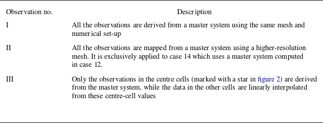
) in the surrounding cells accounts for scenarios where only the centre cells (marked with a star) provide exact observations, while the surrounding values are interpolated to enhance the DA performance. This situation commonly arises in practical applications, where experimental measurements typically capture flow information only at the centre cells, leaving data on the surrounding cells unavailable. Data assimilation that relies solely on velocity measurements from the centre cells would therefore require a relatively dense set of observations, as is demonstrated later. Whether the surrounding-cell velocities are obtained by directly copying the centre-cell values or by interpolating the centre-cell measurements, the resulting observations inevitably contain substantial errors. In this study, we introduce a parameter
 $\sigma \gt0$
to down-weight the observations on the surrounding cells, which significantly reduces the influence of these observational errors and improves the agreement between the assimilated and true flow fields. Notably, the length scales in the mask function are normalised by the local mesh scales
 $\Delta x,\ \Delta y$
and
 $\Delta z$
rather than the commonly defined turbulence scales, since LES inherently involves explicit mesh truncation. Physically, such mesh scales represent the smallest resolved turbulent structures present in LES turbulent systems. The results will demonstrate that synchronisation primarily depends on mesh-based observation density, with the turbulence-scale-based criterion becoming relevant only when the mesh resolution meets DNS requirements. This does not violate the fundamental principle that turbulence synchronisation relies on small-scale information in turbulent systems. In fact, previous studies have predominantly employed DNS, in which the characteristic small-scale structures in the system correspond to the Kolmogorov (Lalescu et al. Reference Lalescu, Meneveau and Eyink2013) or Taylor (Wang & Zaki Reference Wang and Zaki2022) scales. However, in LES, the smallest scales are truncated by the LES mesh filter. The synchronisation criterion naturally shifts to the mesh-based density of the observational data. The observation density
 $\mathcal{S}$
is defined as
 \begin{equation}\mathcal{S}=\sqrt[3]{\frac{N_{\mathit{obs}}}{N_{x}\times N_{y}\times N_{z}}},\end{equation}
where
 $N_{\mathit{obs}}$
is the number of star-marked centre cells and N
x
, N
y
and N
z
are the number of cells in x, y and z directions of the computational domain, respectively. In both the master and slave systems, a periodic boundary condition is applied to the front–back and inlet–outlet surfaces. A constant pressure gradient is imposed in the streamwise direction to achieve the target Reynolds numbers. Both DNS and LES employ the second-order central scheme for spatial discretisation and the second-order backward scheme for temporal discretisation. The time step is adjusted to maintain a maximum Courant number of approximately 0.5. The LES utilise the wall-adapting local eddy-viscosity model for subgrid stress modelling. All computations, including DNS, LES and DA, are performed on the OpenFOAM (www.openfoam.org) platform.
List of case configurations.

*For these cases, mesh resolutions are insufficient for DNS or LES.
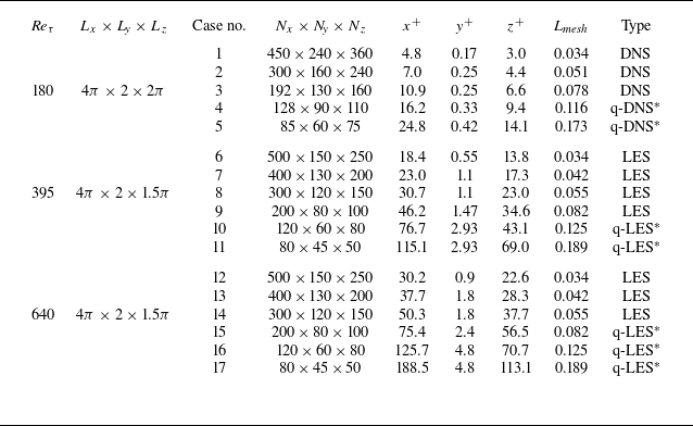
The cases investigated in the present study are summarised in table 1. Three Reynolds numbers are considered with only the case of
 $\textit{Re}_{\tau }= 180$
simulated using DNS. Observations are denoted in different ways as described in table 2. Unless otherwise emphasised, each slave DA system uses the observations from the master system with the same mesh and set-up (observation I). In other words, within a given case number, the only difference between the master and slave systems is the initial condition. However, observations mapped from higher-resolution case (observation II) or interpolated from the down-sampled centre-cell values (observation III) are employed to support the analysis. The computation of each slave system is conducted for different values of
 $\mathcal{S}$
and
 $\sigma$
. Notably, in full synchronisation study (Wang & Zaki Reference Wang and Zaki2022), DNS with identical computational mesh and discretisation scheme is required for both maser and slave to eliminate uncertainties arising from numerical methods. However, this study adopts a ‘weak-constraint’ approach to account for computational uncertainties such as subgrid model errors and discretisation errors, making it more applicable to realistic flow conditions. All master flows are validated against DNS data (Abe, Kawamura & Matsuo Reference Abe, Kawamura and Matsuo2001), while the DNS or LES cases marked with an asterisk fail to accurately capture the mean velocity and fluctuation profiles due to insufficient mesh resolution. These are specially marked with ‘q-’ in the table. Nonetheless, these cases serve as a valuable test case to examine the dependence of modal synchronisation on master flow validity and the impact of significant model and discretisation errors. The assimilation procedure is executed every 10 time steps to minimise storage and computational costs, a sufficient temporal density to avoid affecting the DA results as demonstrated by Wang et al. (Reference Wang and Zaki2022). For each case, 1000 instantaneous flow fields are saved, with modal synchronisation analysis conducted using the final 500 snapshots.
List of observation configurations.

3. Results and discussion
3.1. Synchronisation with sparse observations
In the slave systems, the fluid in unobserved regions – those without direct measurements – also undergoes correlated motion as synchronisation develops. The flow dynamics in these regions remain strongly correlated with the available observational data. Our primary objective is to identify and extract these embedded flow components from the chaotic turbulent system. The master flow is directly integrated into the slave system, maintaining identical mesh resolution and numerical discretisation for each DA case. Observations from both the central and surrounding cells (as shown in figure 2) are sourced directly from the master flow. In the first DA scenario with
 $\sigma =+\infty$
, a single-cell assimilation approach is applied, disregarding observations from surrounding cells. In all slave systems, the initial conditions are deliberately set to differ significantly from those of the master flow, as shown in the first row of figure 3 where case 3 as listed in table 1 is used for demonstration. At the onset of DA, spot defects appear on the velocity contours at the observation sites, reflecting the underdevelopment of global flow in the slave system. The motivation behind the SeVar approach is to achieve global synchronisation of the slave flow by leveraging inherent spatiotemporal correlations. This process unfolds over time, as evidenced in the second row of figure 3, where smooth velocity contours emerge at
 $t^{+}=1000$
. Full synchronisation is defined as the state where pointwise errors (normalised by bulk velocity) are reduced to less than 1 %. The results show that this criterion is satisfied for the entire slave flow at an observation density of
 $\mathcal{S}=0.33$
. However, at lower densities such as
 $\mathcal{S}=0.25$
, while the assimilated flow maintains strong overall similarity to the master flow, discernible pointwise errors persist near the wall region. Further reduction in observation density to
 $\mathcal{S}=0.12$
results in significantly degraded correlation between the assimilated and master flows, with substantial errors distributed across the channel.
Flow fields and error distributions in the slave systems with different densities at
 $\textit{Re}_{\tau }=180$
in case 3 with
 $\sigma =+\infty$
: (a)
 $\mathcal{S}=0.33$
, (b)
 $\mathcal{S}=0.25$
and (c)
 $\mathcal{S}=0.12$
. First row: the initial time step; second row: long time; third row: errors at long time. Contours in the first and second rows denote the vertical velocity of the assimilated slave flows, while the black curves represent the contours of
 $U_{y}/U_{0}=\pm 0.1$
in the DNS master flow.

Asymptotic behaviours of the vertical velocity at
 $y^{+}=15$
in case 3 with
 $\sigma =+\infty$
. (a) Temporal variation at a selected point. First row:
 $\mathcal{S}=0.33$
; second row:
 $\mathcal{S}=0.25$
; third row:
 $\mathcal{S}=0.12$
. (b) Normalised errors at various densities.

The asymptotic behaviours of the assimilated flows are shown in figure 4, where the temporal variation of vertical velocities in a free cell (without observation located) at
 $y^{+}=15$
and the normalised errors are presented. As no observations are available at the selected point, the assimilated slave flow initially exhibits significant deviation from the master DNS data as shown in figure 4(a). In the full-synchronisation case at
 $\mathcal{S}=0.33$
, the DA data rapidly converge to the DNS results, with the two curves overlapping for
 $t^{+}\gt 200$
. While full synchronisation also occurs for
 $\mathcal{S}\gt 0.33$
, such cases are not discussed in this study. For the non-synchronisation case at
 $\mathcal{S}=0.12$
, the two curves evolve rather independently without any correlation that can be discerned in the temporal domain. Focusing on an intermediate density
 $\mathcal{S}=0.25$
, the DA data display strong temporal correlation with the DNS results, though they do not fully coincide. Figure 4(b) further clarifies the asymptotic trends by depicting the normalised errors across different observation densities. At
 $\mathcal{S}=$
0.10 and 0.12, the errors remain consistently high throughout the assimilation period. However, a notable reduction in errors emerges at later times for densities in the range
 $\mathcal{S}=$
0.16–0.25, albeit with residuals still exceeding those of the
 $\mathcal{S}=$
0.33 case. These findings suggest that partial flow recovery occurs in the slave systems for intermediate densities
 $\mathcal{S}= 0.16$
–0.25, even though full synchronisation is unattainable due to insufficient observation density.
Bin-wise correlation of the flows with the master DNS at
 $\textit{Re}_{\tau }= 180$
in case 3: (a)
 $\mathcal{S}=$
0.25, (b)
 $\mathcal{S}=$
0.16 and (c)
 $\mathcal{S}=$
0.12.

The adoption of a
 $3\times 3\times 3$
assimilation cell configuration, weighted by coefficient
 $\sigma$
, is motivated by practical experimental conditions where observational data are typically limited to centre cells. The inclusion of surrounding cells with diminished weighting (reflecting lower confidence) serves to enhance DA, thereby improving flow reconstruction accuracy despite sparse direct measurements. While expanding the assimilation cube to larger dimensions (e.g.
 $5\times 5\times 5$
or beyond) might improve accuracy further, such benefits would be inherently constrained by a threshold determined by surrounding estimation errors. In the present study, the values in the surrounding cells are estimated through linear interpolation of the sparse observations (observation III). The confidence level of these interpolated values is reduced by increasing the coefficient
 $\sigma$
from zero during the DA process. Here, we consider DNS cases at
 $\textit{Re}_{\tau }= 180$
(case 3) with densities
 $\mathcal{S}=$
0.12, 0.16 and 0.25 below the full-synchronisation threshold. To evaluate the similarity between the assimilated flows and the reference DNS data within the assimilation cube, a bin-wise correlation metric is defined as
 \begin{equation}\mathcal{C}_{\mathit{bin}}(y)=\frac{\left\langle \boldsymbol{u},\boldsymbol{u}_{\mathit{DNS}}\right\rangle _{y}}{\left\| \boldsymbol{u}\right\| _{y}\boldsymbol{\cdot }\left\| \boldsymbol{u}_{\mathit{DNS}}\right\| _{y}}.\end{equation}
In this formulation,
 $\boldsymbol{u}_{\mathit{DNS}}$
represents the fluctuating component of the DNS data, with all vector components and cell values within the
 $3\times 3\times 3$
assimilation cube arranged as a single vector. The same vectorisation approach is applied to
 $\boldsymbol{u}$
, which may represent either DA results or interpolated observations. Temporal averaging is performed for each wall-normal position at identical wall distances. Figure 5 presents the wall-normal distribution of
 $\mathcal{C}_{\mathit{bin}}$
. The interpolation accuracy depends strongly on the characteristic length scales of vortical structures at a given observation density. Values of
 $\mathcal{C}_{\mathit{bin}}$
are higher in the channel centre region and decrease progressively towards the channel walls. A particularly rapid decline in
 $\mathcal{C}_{\mathit{bin}}$
is observed in the interpolated field (approximately equivalent to DA
 $\sigma =0$
) within the buffer layer (
 $y^{+}= 10$
–30) where intense small-scale vortical structures are generated. The case
 $\sigma =\infty$
corresponds to single-cell assimilation, where
 $M$
has non-zero values only in the centre cells. This configuration leads to significant improvement in
 $\mathcal{C}_{\mathit{bin}}$
within the viscous sublayer and buffer layer for DA at
 $\mathcal{S}=$
0.25, as demonstrated in figure 5(a). However, this single-cell assimilation approach shows deteriorating correlation performance with sparser observations as evidenced in figures 5(b) and 5(c). The assimilation using
 $\sigma =1$
significantly enhances correlation in both the sublayer and buffer layer across all considered densities. At
 $\mathcal{S}=$
0.12 and 0.16, this correlation substantially exceeds that observed with
 $\sigma =\infty$
, while at
 $\mathcal{S}=$
0.25, it becomes marginally lower in the region beneath the buffer layer (
 $y^{+}= 1$
–20). These findings demonstrate that the degree of synchronisation exhibits a positive correlation with
 $\mathcal{C}_{\mathit{bin}}$
. More importantly, DA employing interpolated observations with an appropriately selected
 $\sigma$
value proves highly effective in enhancing the synchronisation level, thereby improving the accuracy of global flow reconstruction from sparse observations. Conversely, figures 5(b) and 5(c) reveal that DA implementation in non-synchronised regimes results in even lower
 $\mathcal{C}_{\mathit{bin}}$
values than direct interpolation, particularly within the logarithmic layer. This indicates that the current DA framework fails to achieve global flow reconstruction when non-synchronisation dominates at the present observation density. While using a finite
 $\sigma$
value effectively increases the equivalent observation density
 $\mathcal{S}$
and may appear advantageous for flow reconstruction, it is crucial to recognise that an optimal
 $\sigma$
exists for each specific density. This is evidenced by the counterexample of
 $\sigma =0$
, where the slave flow in the assimilating cube converges towards the direct interpolation result. Furthermore, the
 $\mathcal{C}_{\mathit{bin}}$
values in the
 $y^{+}= 1$
–20 region shown in figure 5(a) suggest that smaller
 $\sigma$
values should be employed at higher observation densities.
Streamwise variations of the wall-normal velocity component at
 $y^{+}=40$
and
 $\textit{Re}_{\tau }= 180$
in case 3 for
 $ \sigma = 1$
: (a)
 $\mathcal{S}=$
0.12 and (b)
 $\mathcal{S}=$
0.16.

Figure 6 presents the streamwise variation of wall-normal velocities at a selected point, with
 $\mathcal{S}= 0.12$
and 0.16 selected for demonstration. For each density, two assimilated slave systems with uncorrelated initial conditions are compared. The two slave systems exhibit nearly identical streamwise velocity variations at
 $\mathcal{S}= 0.12$
, with only minor discrepancies apparent in figure 6(a). Notably, these assimilated velocity distributions capture the essential features of the real flow significantly better than the interpolation when compared with DNS data. When the density increases to
 $\mathcal{S}= 0.16$
, the two slave flows overlap completely, though noticeable differences from the master DNS data emerge as shown in figure 6(b). This state does not precisely reproduce the interpolated field, but rather generates a new state that more closely resembles the DNS results. This finding demonstrates that global flow-field reconstruction remains possible even when the interpolated observations capture substantially different flow details. The primary discrepancy between the assimilated slave flow and master DNS occurs at the velocity peak location. This feature is particularly susceptible to being filtered out by sparse observations and cannot be adequately recovered through interpolation. While this issue also occurs in perfect-observation DA systems, its impact diminishes when using higher observation densities or smaller
 $\sigma$
values.
The ESPOD modes in the master system at
 $\mathcal{S}=0.25$
with
 $\sigma =+\infty$
in case 3. Vertical component of the velocity normalised by the maximal value is shown (a–c) at different wall distances y
+
, (d–f) at different Strouhal numbers St and (e–i) at different POD orders i.

3.2. Modal synchronisation identification
The synchronised components of the flow, which exhibit strong correlations with the sparse observations, are identified using the ESPOD method, as detailed in § 2.2. For each case, 500 snapshots are analysed. The data are divided into segments of 50 consecutive instantaneous fields for DFT computation, with a 40-field overlap between adjacent segments, resulting in a total of 46 segments for POD analysis. As an illustration, figure 7 presents the ESPOD modes in case 3 in the master system at an observation density of
 $\mathcal{S}=$
0.25. These modes were obtained by extending the SPOD modes of the observational data layer by layer to different wall-parallel planes. Notably, in other slave systems under the same case label and DA parameters, correlated flows are extracted by projecting onto these ESPOD modes as indicated by (2.18). Consequently, the spatial distributions of the correlated modes across different slave systems are fully consistent with those shown in figure 7. According to the ESPOD definition, the modes in figure 7 share identical temporal coefficients with the corresponding SPOD modes of the observational data as shown in (2.16). This implies that the global flow excited by the sparse observations in this study is extracted through temporal correlation, with no direct spatial-scale relationship. As seen in figure 7(a–c), the same observations excite distinctly different global flow structures at different wall distances, with the spatial scale decreasing as the wall distance decreases. This is consistent with the distribution characteristics of turbulent scales in channel flows. At the same wall distance, the spatial scale of the modes decreases significantly with increasing frequency, as shown in figure 7(d–f). A key insight from these results is that although sparse observations contain only large-scale flow information, they can excite a variety of small-scale vortical structures during the DA process, with both sharing similar temporal evolution patterns. This phenomenon does not arise from direct spatial correlation between the observations and the global flow. Rather, it is initially excited by temporal correlation, which induces the formation of small-scale structures downstream of the observation locations, and subsequently propagates through synchronisation mechanisms to excite small-scale global modes. High-frequency sampling of observations is a crucial prerequisite, as also demonstrated by Wang et al. (Reference Wang and Zaki2022). The role of POD in this context is mainly to filter the Fourier modes, helping to determine whether the excited flows in the master and slave systems exhibit temporal correlation. As shown in figure 7(g–i), different POD orders show minimal differences in the spatial scales of the modes but differ primarily in the level of noise. Therefore, using low-order POD modes is more appropriate for evaluating flow synchronisation characteristics across different frequencies.
Energy evolution of the ith-order ESPOD modes
 $\hat{\boldsymbol{\psi }}$
evaluated at
 $y^{+}=2$
with
 $\mathcal{S}$
= 0.25 and
 $\sigma =+\infty$
in case 3: (a) St = 0.17 and i = 5; (b) St = 0.87 and i = 5; (c) St = 1.74 and i = 20; (d) St = 0.17 and i = 30.

The dynamic characteristics of synchronised modes can be illustrated through their kinetic energy evolution, as depicted in figure 8. The kinetic energy is normalised by the total kinetic energy at the corresponding wall distance in the master system. We examine two slave systems that differ solely in their initial conditions during the assimilation process. As demonstrated in figure 8, the energy evolution of slave-system modes closely matches that of the corresponding ESPOD modes in the master system, regardless of the Strouhal number and mode order. Notably, the slave modes exhibit remarkable insensitivity to initial conditions, as evidenced by the near-perfect overlap between the two slave-system curves, even at St = 1.74 and for higher-order modes (up to i = 20) as shown in figure 8(a–c). However, a gradual decline in curve similarity emerges with further increases in mode order, even at low Strouhal numbers. The observed similarity in modal energy evolution confirms successful modal synchronisation in the slave system, achieved via sparse-data-driven assimilation. This synchronisation typically develops alongside the slave system's dynamic evolution, which loses dependence on its initial state. Nevertheless, compared with the master-system reference, each synchronised mode exhibits reduced energy and becomes more pronounced at higher Strouhal numbers. This suggests that high-frequency, small-scale structures are more challenging to recover within the modal synchronisation framework.
The similarity in mode energy evolution can be quantified using the cross-correlation coefficient
 $\mathcal{C}$
of the ESPOD mode coefficients for each frequency and mode order, as defined in (2.20). This approach is justified because synchronisation involves the same modes in both the slave and master systems. Figure 9 presents the calculated values of
 $\mathcal{C}$
at various wall distances for
 $\mathcal{S}$
= 0.25. Regions with high
 $\mathcal{C}$
values indicate strong similarity in mode energy evolution, and a threshold of
 $\mathcal{C}\gt 0.9$
is adopted to define modal synchronisation. The results reveal that modal synchronisation is more readily achieved in the channel centre than near the wall. Notably, while the Strouhal number influences mode energy, it does not play a decisive role in modal synchronisation. However, modal synchronisation breaks down at higher mode orders (
 $i\gt 40$
), as these modes predominantly represent random noise and contain substantially less energy than the synchronised modes. Additionally, modal synchronisation tends to fail at moderate and high mode orders near St = 0, where the modes correspond to large-scale flow variations that extend across multiple data segments as captured by ESPOD using a finite-length DFT window. The data in figure 8 correspond to the (St, i) parameters marked by the yellow circles in figure 9(d), all of which satisfy the
 $\mathcal{C}\gt 0.9$
synchronisation criterion.
Cross-correlation of the mode coefficients in the slave and master systems with
 $\mathcal{S}$
= 0.25 and
 $\sigma =+\infty$
in case 3: (a)
 $y^{+}$
= 150, (b)
 $y^{+}$
= 60, (c)
 $y^{+}$
= 15 and (d)
 $y^{+}$
= 2. Modal synchronisation is defined when
 $\mathcal{C}\gt 0.9$
. The yellow circles A, B, C and D represent the (St, i) parameters extracted from Figures 8(a)–8(d), respectively.

For the same DA case with
 $\mathcal{S}$
= 0.16, the energy evolution and cross-correlation of mode coefficients are analysed, with focus restricted to the channel centre. Consistent with the earlier findings, modal synchronisation is achieved primarily near the channel centre (
 $y^{+}$
= 150). Although minor discrepancies in mode energy evolution are evident between the two slave systems as observed in figures 10(a) and 10(b), a substantial region with
 $\mathcal{C}\gt 0.9$
persists as shown in figure 10(c). The results indicate that the transition between modal-synchronisation and non-synchronisation states occurs gradually rather than abruptly. Notably, as demonstrated in figure 10(d), certain individual modes at
 $y^{+}$
= 60 still exhibit modal synchronisation characteristics. However, this study primarily focuses on clearly established cases of modal synchronisation, particularly those where the leading-order ESPOD modes satisfy the 0.9 correlation criterion across most Strouhal numbers.
Modal synchronisation at
 $\mathcal{S}$
= 0.16 and
 $\sigma =+\infty$
in case 3. Energy evolution of the ith-order ESPOD modes
 $\hat{\boldsymbol{\psi }}$
evaluated at
 $y^{+}$
= 150: (a) St = 0.08 and i = 2; (b) St = 0.6 and i = 2. Cross-correlation of the mode coefficients between the slave and master systems at (c)
 $y^{+}$
= 150 and (d)
 $y^{+}$
= 60.

The failure of modal synchronisation in ESPOD modes under low observation density stems from incomplete information transfer between observations and the slave flow within the DA framework. This phenomenon primarily manifests as a velocity slip between observation points and surrounding fluid parcels. Under sparse observation conditions, the acquired information predominantly captures large-scale vortical structures, which must then be propagated to adjacent fluid through the existing nudging-like assimilation strategy. While the global Fourier mode injection method employed by Nikolaidis & Ioannou (Reference Nikolaidis and Ioannou2022) demonstrates theoretical advantages in this regard, the present study focuses on more realistic observation, mirroring practical experimental scenarios where data acquisition is limited to spatially sparse locations. A straightforward strategy for enhancing modal synchronisation involves minimising velocity slip by incorporating information from neighbouring regions of the master flow. This is achieved through finite values of the coefficient
 $\sigma$
, which define
 $3\times 3\times 3$
assimilation cells with spatially decaying weights from the centre cell. It is noteworthy that although observations in both centre and surrounding cells are directly obtained from the master system, effectively increasing the observation density, this approach retains practical relevance for experimental applications. In such cases, surrounding values can be reasonably approximated through interpolation or duplication techniques.
Examining case 14 shown in table 1, figure 11 presents the cross-correlation maps of the mode coefficients with the observation density
 $\mathcal{S}$
= 0.14. A LES model is employed for both the master and slave systems at
 $\textit{Re}_{\tau }=640$
to assess the influence of model imperfections on modal synchronisation. Unlike previous studies, which typically required the master and slave systems to employ identical meshes and computational settings in order to achieve turbulence synchronisation, the present work further investigates the effects of numerical discrepancies. Specifically, we use the mapped fields from a higher-resolution LES case (case 12) as the master flow, as shown in the second and fourth columns of figure 11. Initial results demonstrate that with this observation density and
 $\sigma = \infty$
, the system fails to achieve modal synchronisation due to the insufficient observation density. From these results, it is also clearly evident that using finite values of
 $\sigma$
can significantly enhance the degree of modal synchronisation. Reducing the
 $\sigma$
value effectively increases the density of available observational data. However, it should be noted that this method of increasing data density does not directly reduce the scale of turbulent structures captured by the observations. Instead, it efficiently increases the assimilated volume fraction of the computational domain. As noted by Clark Di Leoni et al. (Reference Di Leoni, Mazzino and Biferale2020), the nudged volume fraction in physical space is an important parameter for turbulent synchronisation. Here, we interpret the influence of this parameter as the velocity slip between observation points and the surrounding fluid parcels. Another notable feature is the consistently lower correlation when using the mapped master flows from the higher-resolution mesh at all wall distances. Although the master flow mapped from the higher-resolution mesh occupies each mesh element in the slave system, minor interpolation errors are introduced during the mapping process. These errors reduce the energy proportion of synchronised modes during the ESPOD decomposition, leading to a decrease in
 $\mathcal{C}$
value shown here. However, as demonstrated later, this reduction in correlation does not fundamentally affect the flow synchronisation characteristics. In other words, the turbulent synchronisation behaviour remains unchanged while only the strictly correlated flow components are diminished within the current ESPOD framework.
Cross-correlation of the mode coefficients in the slave and master systems with
 $\mathcal{S}$
= 0.14 at
 $\textit{Re}_{\tau }=640$
in case 14: (a–d)
 $\sigma =0$
, (e–h)
 $\sigma =1.5$
and (i–l)
 $\sigma =2.5$
. First and third columns: using master data computed from higher-resolution mesh of case 12; second and fourth columns: using master data computed from the same mesh.

Synchronisation map constructed based on the cases 3, 8, 12 and 14. The filled symbols represent the full-synchronisation state, the open symbols denote the modal-synchronisation state, while the symbols with cross denote the non-synchronisation state. The black dashed lines indicate the approximate boundary between the three different regimes.

Through comprehensive analysis of DA cases across varying Reynolds numbers, observation densities and
 $\sigma$
values, a synchronisation map is constructed, as presented in figure 12. In this framework, full synchronisation is achieved only when the flow satisfies the synchronisation criterion on all wall-parallel planes. In contrast, modal synchronisation is identified when the criterion is met on at least one wall-parallel plane, reflecting partial yet coherent alignment of dominant flow structures. The
 $\mathcal{S}{-}\sigma$
parameter space can be categorised into three distinct regimes representing full synchronisation, modal synchronisation and non-synchronisation states. A key finding is that the threshold boundaries between these regimes are independent of the predictive model, Reynolds number and mesh resolution. This contrasts with prior studies, which demonstrated that full synchronisation primarily depends on the length scale of the observations and the Kolmogorov scale in the flow system. While the full-synchronisation criterion should be also applicable in the present study for DNS cases, its practical evaluation is complicated by the challenge of determining the observational length scales in these strongly anisotropic wall-bounded flows. Figure 12 reveals that observation density serves as the fundamental metric for assessing synchronisation within the current DA framework, given that the parameter
 $\sigma$
also represents an equivalent density measure. This interpretation is intuitive because only a portion of the turbulence spectrum prevails in the master LES system. Consequently, the observation density governs the degrees of freedom in the slave flows that can be adjusted during the DA process, provided the smallest turbulence scale in the flow is finer than that which the mesh resolution can resolve. In other words, the Kolmogorov-scale or Taylor-scale criterion for full synchronisation, previously established for homogeneous or channel flows, represents the limiting case of the present density-based criterion when mesh resolution is progressively refined and the predictive model transitions to DNS. This assertion is supported by the results in figure 13, which compares the equivalent length scales resolved by sparse observations with twice the Taylor microscale, i.e. a relevant metric for assessing synchronisation in turbulent channel flows proposed by Wang & Zaki (Reference Wang and Zaki2022). The Taylor microscale is computed using DNS data from Abe et al. (Reference Abe, Kawamura and Matsuo2001) and the anisotropic turbulence formulation by Pope (Reference Pope2000), while the equivalent observational scale is estimated as
 \begin{equation}\varLambda _{\mathit{obs}}\approx \frac{u_{\tau }}{\mathcal{S}\nu }\sqrt{\left(\frac{L_{x}}{N_{x}}\right)^{2}+\left(\frac{L_{y}}{N_{y}}\right)^{2}+\left(\frac{L_{z}}{N_{z}}\right)^{2}}=\frac{u_{\tau }}{\mathcal{S}\nu }L_{\textit{mesh}},\end{equation}
where
 $u_{\tau }$
represents the wall friction velocity and
 $L_{\textit{mesh}}$
defines the mesh scale. A full-synchronisation density of
 $\mathcal{S}=0.33$
is selected, yielding equivalent length scales
 $\varLambda _{\mathit{obs}}=$
41.2, 63.8 and 103.4 for
 $\textit{Re}_{\tau }=$
180 (case 3), 395 (case 8) and 640 (case 14), respectively. Case 3 approximately satisfies the Taylor-scale criterion proposed by Wang & Zaki (Reference Wang and Zaki2022), while sparse observations are sufficient to synchronise all scales in the inertial sublayer. In contrast, the LES cases 8 and 14 resolve only a subset of the scales in the inertial sublayer and do not meet the Taylor-scale criterion. However, they still fall within the full-synchronisation regime in the present study. Notably, full-scale alignment in the full-synchronisation regime cannot be achieved with observation cases II and III, because the interpolation errors in the observations cannot be fully compensated by any momentum forcing within the current DA framework. A key reason for this limitation is that the slave flow inherently satisfies the continuity condition, whereas the mapped observations do not. Nevertheless, the final converged state of the slave system under this regime is independent of the initial conditions; that is, slave systems initialised differently ultimately align with each other across all scales, as also reported by Li, Tian & Li (Reference Li, Tian and Li2022). Another notable phenomenon is that when observation configuration III is employed, the flows tend to achieve full synchronisation more readily at smaller values of
 $\sigma$
. This may be attributed to the fact that such down-sampling in physical space constrains the slave system into a state devoid of fine-scale vortex structures. As a result, the flow field possesses fewer degrees of freedom, making it more susceptible to full synchronisation. However, this tendency gradually weakens as
 $\sigma$
increases.
Taylor scales of the turbulence at different Reynolds numbers and wall distances. The horizontal lines represent the equivalent length scales captured at
 $\mathcal{S}=0.33$
in cases 3, 8 and 14 for each Reynolds number.

To further examine the dependence of flow synchronisation on turbulent scales and mesh resolution, we analysed the synchronisation characteristics under different mesh scales for each Reynolds number, i.e. for all cases listed in table 1. To ensure consistent comparisons, all cases were configured with
 $\sigma = 0$
and with observation configuration I. The relative mesh scale,
 $L_{\textit{mesh}},$
is defined in (3.2), and the corresponding computational cases with varying grid scales are provided in table 1. First, considering the DNS cases at
 $\textit{Re}_{\tau }= 180$
, the mesh employed in case 3 meets the Taylor-scale criterion established by Wang & Zaki (Reference Wang and Zaki2022), meaning it approaches the resolution threshold to resolve all energy-containing flow structures and thereby enables the full-synchronisation regime. The corresponding mesh scale is
 $L_{\textit{mesh}}= 0.078$
. However, when the mesh resolution is further increased, the same observation density is able to capture smaller turbulent scales (i.e.
 $\varLambda _{\mathit{obs}}$
), even though no smaller energy-containing turbulent structures are present in the flow. This implies that at higher mesh resolutions, a lower observation density is sufficient to attain the full-synchronisation regime. From figures 13 and 14, it can be estimated that
 $L_{\textit{mesh}}$
= 0.078 and
 $\mathcal{S}=$
0.14 are approximately sufficient to achieve full synchronisation. If the flow is to remain fully synchronised at increased mesh resolutions,
 $\varLambda _{\mathit{obs}}$
should remain constant. Therefore, according to (3.2), it follows that
Synchronisation map using different meth resolutions with
 $\sigma =0.$
The filled symbols represent the full-synchronisation state, the open symbols denote the modal-synchronisation state, while the symbols with cross denote the non-synchronisation state. The black dashed lines indicate the approximate boundary between the three different regimes. The blue solid line represents the slope of (3.3). The DNS/LES and q-DNS/q-LES are separated by
 $L_{\textit{mesh}}\approx 0.082$
.

 \begin{equation}\frac{\mathcal{S}}{L_{\textit{mesh}}}\approx \frac{u_{\tau }}{\nu \boldsymbol{\cdot }\varLambda _{\mathit{obs} (\mathcal{S}=0.14)}}.\end{equation}
This relationship indicates that a straight line with this slope separates the regimes of full synchronisation and modal synchronisation. The results for
 $\textit{Re}_{\tau }=180$
in figure 14 corroborate this observation: in cases 1 and 2, the minimum observation density required for the flow to achieve full synchronisation lies just above this sloped line, whereas below it, the system transitions into the modal synchronisation regime. It is noteworthy that, according to the analysis in § 3.2, achieving full synchronisation requires reaching a certain assimilated volume fraction. Consequently, at higher grid resolutions, the reduced observation density leads to a lower assimilated volume fraction, which shifts the threshold for full synchronisation away from the reference line. A similar trend is observed in figure 14. In this case, when the mesh resolution is coarse in the range
 $L_{\textit{mesh}}\lt 0.09$
, the threshold observation density for the three regimes remains relatively constant. This occurs because, for low-resolution grids, the DNS effectively behaves as an implicit LES, with the computational grid acting as an implicit filter. In such a scenario, the smallest energy-containing vortices in the turbulent system are no longer characterised by the Taylor scale, but rather by the mesh filter scale. At a fixed observation density, the ratio of the observational length scale to the scale of the smallest energy-containing vortices remains constant. It is this scale ratio that governs the synchronisation behaviour of the flow. This interpretation is further supported by the cases at
 $\textit{Re}_{\tau }=$
395 and 640, where the threshold observation density similarly remains nearly constant for
 $L_{\textit{mesh}}\lt 0.09$
. However, when mesh resolution is increased beyond
 $L_{\textit{mesh}} \lt 0.05$
, the slope change observed in the DNS case does not appear. This is because the LES framework inherently includes smaller-scale turbulent structures; increasing mesh resolution must therefore be accompanied by a corresponding reduction in the turbulence scale resolved by the mesh, so as to preserve the constancy of the ratio between the observational length scale and the smallest energy-containing turbulence scale in the system. According to the statistical data presented in figure 14, the boundaries of the three synchronisation regimes across different Reynolds numbers consistently lie near S = 0.14 and 0.06. However, when the mesh resolution becomes very coarse (i.e.
 $L_{\textit{mesh}}\gt 0.09$
), these boundaries begin to deviate from the constant values, indicating that a higher observational density is required to achieve either full or modal synchronisation. At such mesh resolutions, turbulent statistics obtained via DNS or LES also exhibit significant deviations from the accurate values.
These findings indicate that, beyond the previously established regime of full turbulence synchronisation, a state of modal synchronisation also exists in data-assimilated turbulent systems under sparse observations. In both DNS and LES frameworks, the criterion for achieving full synchronisation depends on the ratio between the observational scale and the smallest energy-containing scale in the slave system. When the computational mesh satisfies DNS requirements, the slave system in physical space achieves full synchronisation with the criterion for the observation data coinciding with the Taylor-scale criterion proposed by Wang & Zaki (Reference Wang and Zaki2022). In contrast, when mesh resolution only meets LES standards, the smallest turbulent scale in the slave system becomes the mesh filter scale, and the synchronisation criterion shifts to observation density, i.e. effectively the ratio of the mesh filter scale to the observational scale. The emergence of modal synchronisation across all systems is predominantly governed by this observation density. Moreover, when mesh resolution falls below LES requirements, the synchronisation behaviour of the flow field deviates from the above criteria.
3.3. Delay-coordinate assimilation
Based on the preceding analysis, incorporating historical information from limited observations emerges as one of the most effective strategies for mitigating discrepancies between slave and master flows under low observation densities. While positioning observations at velocity peak locations would maximise assimilation accuracy, this approach is inherently impractical due to the absence of a priori knowledge of the instantaneous flow field. In practical applications such as LPT measurements, observation sites are typically randomly distributed across the flow domain. In such scenarios, leveraging the historical variation of velocity offers a viable alternative: through flow convection, it implicitly integrates information from adjacent regions and past velocity peaks that may not be captured at the current time step. This approach thereby enhances assimilation performance by spatially and temporally extending the influence of sparse measurements. The present study employs a delay-coordinate strategy, which incurs negligible additional computational cost compared with conventional DA methods. Unlike nudging techniques that directly introduce feedback terms into the momentum equations, the proposed SeVar framework requires modifications to the adjoint momentum equations (see Appendix A for details). Here, observations are considered at the current time step (
 $\kappa$
) as well as the two preceding steps (
 $\kappa -1$
,
 $\kappa -2$
):
 \begin{align}\frac{\boldsymbol{V}}{{\delta} t}+\boldsymbol{\nabla }\boldsymbol{U}\boldsymbol{\cdot }\boldsymbol{V}&-\left(\boldsymbol{U}\boldsymbol{\cdot }\boldsymbol{\nabla }\right)\boldsymbol{V}-\boldsymbol{\nabla }\boldsymbol{\cdot }\big[\nu _{\textit{eff}}\big(\boldsymbol{\nabla }\boldsymbol{V}+\left(\boldsymbol{\nabla }\boldsymbol{V}\right)^{T}\big)\big]+\frac{1}{\rho }\boldsymbol{\nabla }q \nonumber \\&\quad +\frac{2\xi M}{U_{0}^{2}}\left[\left(\boldsymbol{U}''-\boldsymbol{U}_{\mathit{obs}}''\right)+\left(\boldsymbol{U}'-\boldsymbol{U}_{\mathit{obs}}'\right)+\left(\boldsymbol{U}-\boldsymbol{U}_{\mathit{obs}}\right)\right]=0,\end{align}
where
 $\boldsymbol{U}'$
and
 $\boldsymbol{U}_{\mathit{obs}}'$
denote the assimilated flow and the observations, respectively, at the previous observational time
 $t_{\mathit{obs}}^{(\kappa -1)}$
, while
 $\boldsymbol{U}''$
and
 $\boldsymbol{U}_{\mathit{obs}}''$
correspond to those at
 $t_{\mathit{obs}}^{(\kappa -2)}$
. Notably, the delay-coordinate assimilation approach does not necessitate additional data or supplementary observation sites; instead, it leverages the same observational resources employed in conventional DA strategies. Furthermore, given the minimal objective residuals, the delay-coordinate strategy is only meaningful when
 $0\lt \sigma \lt \infty$
in the surrounding cells of the assimilating cube. This approach integrates historical data into the current assimilation time, rather than considering a long evolution trajectory as done in 4DVar. Following the optimisation proposed by Pazo, Carrassi & Lopez (Reference Pazo, Carrassi and Lopez2016), only three time instants are incorporated, as excessive historical data have been shown to diminish the improvement in DA results.
Streamwise variations of the wall-normal velocity component at
 $y^{+}=40$
in case 14 using observation III and
 $\mathcal{S}=$
0.14. The DA is performed with (a)
 $\sigma = 0.5$
, (b)
 $\sigma =1.5$
and (c)
 $\sigma = 2.5$
. The dark yellow circles denote the direct interpolation, duplicated in each subfigure for comparison.

All the following analysis is performed with case 14 using observation configuration III (table 2) at
 $\textit{Re}_{\tau }= 640$
. This case serves as a representative example of weak-constraint DA, where the master flow cannot be fully reproduced by any predictive model, being significantly different from those examined in previous studies (Lalescu et al. Reference Lalescu, Meneveau and Eyink2013; Wang & Zaki Reference Wang and Zaki2022; Li et al. Reference Li, Zhang, Zhou, He and Liu2024). The configuration also serves as a benchmark test, simulating real-world applications where measurement data are employed as observations. Figure 15 presents the streamwise variation of wall-normal velocities at a selected point for DA cases with and without the delay-coordinate strategy. The observation density is fixed at
 $\mathcal{S}=$
0.14, which lies within the modal-synchronisation regime for
 $\sigma = 0.5$
, 1.5 and 2.5. Since the direct interpolation from the down-sampled observations fails to capture fundamental flow characteristics, we focus on DA approaches that demonstrate improved global feature recovery capabilities. Each subfigure compares DA results using perfect observations (configuration I) with interpolated observations (configuration III) at corresponding
 $\sigma$
values. When
 $\sigma$
approaches infinity, both perfect and interpolated observations produce identical DA results, as the assimilation converges to a single-cell scenario where the observations become equivalent. However, the agreement between these two cases does not monotonically improve as
 $\sigma$
increases from 0.5 to 2.5. Notable deviations between the DA results with interpolated observations (blue curve) and those with perfect observations (open circles) are observed at
 $\sigma$
= 0.5 (figure 15a
) and
 $\sigma$
= 2.5 (figure 15c
), while optimal agreement occurs at
 $\sigma$
= 1.5 (figure 15b
). This behaviour suggests the existence of an optimal
 $\sigma$
that minimises DA errors induced by observation interpolation. Although the delay-coordinate strategy significantly enhances velocity peak recovery, it also generates more spurious peaks as
 $\sigma$
decreases.
Velocity snapshots and temporal correlations of the interpolated and assimilated slave flows in case 14 using observation III. Parameter values are indicated above each subfigure for clarity.

To more comprehensively evaluate the enhanced performance of the proposed DA framework incorporating interpolated assimilation and delay-coordinate strategies, figure 16 presents both instantaneous snapshots and temporal correlations of the assimilated fields under varying observation densities and
 $\sigma$
values. The temporal correlation is calculated as the cross-correlation between the target flow field and the LES reference data using a sliding-window approach with a window size of 50 instantaneous fields and 50 % overlap. Figure 16(a) displays the LES reference snapshot for comparison. At each observation density, sparse observations are interpolated onto the global mesh to generate the master interpolated flows, as shown in figure 16(b–d). The interpolation process primarily captures large-scale flow patterns (evident in the upper halves of each subfigure), with temporal correlations remaining near unity at observation sites but decreasing sharply elsewhere. The DA substantially improves the flow fields by reconstructing vortical structures and enhancing temporal correlations. Notably, high correlation values are observed in slender regions downstream of observation sites. As demonstrated in figure 16(e–g), DA with
 $\sigma = 0$
yields the highest temporal correlation across all densities, though with noticeable noise (to be discussed later). Increasing
 $\sigma$
to 1.5 adversely affects DA performance as shown in figure 16(h–j), but this effect diminishes rapidly with increasing observation density. Particular attention should be given to the delay-coordinate assimilation cases in figure 16(k–m), which show marked improvement at
 $\mathcal{S}= 0.1$
but only marginal noise reduction at
 $\mathcal{S}= 0.14$
and 0.2. Importantly, while
 $\mathcal{S}\geq 0.14$
with
 $\sigma = 1.5$
lies within the modal-synchronisation regime (figure 12),
 $\mathcal{S}= 0.1$
with
 $\sigma = 1.5$
approaches non-synchronised conditions. This suggests a preliminary conclusion that when the slave system falls in the modal-synchronisation regime, the delay-coordinate interpolated assimilation strategy with
 $\sigma \gt 0$
can effectively reconstruct global flow dynamics from sparse observations. However,
 $\sigma =0$
performs inferiorly to
 $\sigma =\infty$
at high observation densities due to introduced interpolation errors.
Synchronisation maps at various densities and wall distances in case 14 using observation III: (a)
 $\mathcal{S}= 0.1$
, (b)
 $\mathcal{S}= 0.14$
and (c)
 $\mathcal{S}= 0.2$
. Half-filled circles indicate full or modal synchronisation; circles with cross indicate non-synchronisation. Red circles highlight the parameter sets used for the energy comparison.

To further substantiate the preceding argument, synchronisation maps derived from interpolated assimilation data are re-evaluated on each wall-parallel plane as illustrated in figure 17. This figure does not differentiate between full synchronisation and modal synchronisation across all planes, since even in the full-synchronisation regime the slave flow cannot perfectly match the master flow. Rather, it illustrates the second scenario of full synchronisation, where multiple slave systems converge to mutually identical states. This possibility warrants further investigation through additional computational examples. The comparison of its overall synchronisation map with other cases has been shown in case 14 and observation III in figure 12. It can be observed that the synchronisation characteristics under this observation configuration are generally consistent with other cases. Figure 18 presents the streamwise wave spectra computed from the streamwise velocity component at
 $y^{+}= 50$
and 600. Since the master LES data are interpolated from a finer mesh, the spectra display an upward trend at high wavenumbers due to interpolation artefacts. In contrast, interpolation from sparse observations leads to severe spectral degradation, attributable to the filtering of numerous vortical structures. This manifests as a reduction in power spectral density across most wavenumbers, except at the high-wavenumber range where interpolation errors dominate. Notably, all spectral curves of the assimilated flow exhibit anomalous growth at high wavenumbers, consistent with the nudging results reported by Clark Di Leoni et al. (Reference Di Leoni, Mazzino and Biferale2020). Our analysis focuses on the spectral range below
 $k_{x}\lt 8$
, where the current DA framework operates effectively. As the
 $\sigma$
value increases, each spectral curve demonstrates attenuated power spectral density at relatively high wavenumbers, with this attenuation being weakened progressively at lower wavenumbers. This behaviour clearly indicates that relaxed weighting for surrounding cells primarily influences small-scale structures. This is reasonable since large-scale vortices are already captured by the sparse observations. The key conclusion drawn from figure 18 is that the optimal
 $\sigma$
for spectral reproduction within the present interpolated delay-coordinate DA framework lies near the modal synchronisation/non-synchronisation threshold, as demarcated by the oblique lines in figure 17. However, the precise positioning of
 $\sigma$
within this transitional regime should not be overinterpreted, as the shift from modal synchronisation to non-synchronisation constitutes a gradual rather than abrupt transition. The above argument can be explained through the trade-off between error suppression effects and modal synchronisation strength. Given that modal synchronisation depends solely on equivalent density, it follows that neither delay-coordinate nor weighting-relaxation strategies prove effective for flow systems firmly within the non-synchronisation regime, as these approaches do not increase the number of observation sites involved in the DA process.
(a–f) Streamwise wave spectra computed from the streamwise velocity component in case 14 using observation III. Arrows indicate the optimal
 $\sigma$
value in each subfigure. Parameter values are listed above each subfigure. PSD, power spectral density.

The underlying mechanism for these flow reconstruction improvements can be elucidated through examining energy modifications in the synchronised modes. As representative cases, we analyse the densities and wall-parallel planes, as indicated by filled and open red circles in figure 17, respectively. Figure 19 displays the corresponding energy ratios
 $\mathscr{r}$
relative to the reference LES data as defined in (2.21). Only the leading modes for each frequency are shown, as the remaining synchronised modes exhibit similar trends. The cases with
 $\sigma = 0$
are selected as the benchmark for comparison since they exhibit the highest temporal correlation (figure 16), despite introducing undesirable interpolation errors across all observation densities. Notably, the delay-coordinate approach demonstrates limited effectiveness when
 $\sigma = 0$
, as the contribution of historical data to the adjoint source in (3.4) becomes negligible, being distinct from the nudging mechanism (Pazo et al. Reference Pazo, Carrassi and Lopez2016). The assimilation results show rapid decay with increasing frequency, indicating that the current DA framework cannot adequately reproduce the energy levels of small-scale structures, even when modal synchronisation is achieved. Importantly, the observed high-frequency decay in correlation coefficient
 $\mathscr{r}$
does not correspond to a similar power spectral density reduction in the slave flows (figure 18), as interpolation errors introduce substantial flow components that remain uncorrelated with synchronised modes. For clarity, datasets showing faster attenuation with increasing
 $\sigma$
without delay coordinate are omitted from figure 19 to avoid excessive curve clustering. The analysis focuses primarily on the delay-coordinate DA results, which demonstrate significantly improved correlation coefficients
 $\mathscr{r}$
in the Strouhal number range
 $St= 1.5$
–3.5 across different
 $\sigma$
values compared with the
 $\sigma = 0$
baseline. Remarkably, the optimal
 $\sigma$
values (indicated by arrows) show excellent agreement with those identified in figure 18 at y
+ = 600, and consistently align near the modal synchronisation/non-synchronisation threshold at all wall distances. This finding strongly supports our earlier argument regarding flow reconstruction improvement within the modal-synchronisation regime. Based on the Taylor's frozen hypothesis, we estimate that flow structures with
 $St\approx 3$
correspond to a streamwise wavenumber
 $k_{x}\approx 3$
in the current flow configuration. Given that delay-coordinate assimilations show minimal discrepancies in the
 $k_{x}= 1$
–3 range in figure 18, the observed
 $\mathscr{r}$
increase suggests kinetic energy transfer from uncorrelated components to synchronised modes, while maintaining nearly constant total energy in this frequency band. Although the weighting relaxation strategy accelerates
 $\mathscr{r}$
decay at
 $St\gt 3.5$
, particularly at y
+ = 600, the DA process paradoxically benefits from this uncorrelated component attenuation. This effect ultimately yields optimal wave spectra in the slave flows when using the same
 $\sigma$
values.
Energy ratios of the synchronised modes at different wall distances in case 14 using observation III, as indicated by red in figure 17: (a)
 $\mathcal{S}= 0.1$
, (b)
 $\mathcal{S}= 0.14$
and (c)
 $\mathcal{S}= 0.2$
. Arrows indicate the optimal
 $\sigma$
value in each subfigure.

4. Conclusions
This study employs the SeVar technique to reconstruct global velocity fields in turbulent channel flow using sparse, randomly distributed observations within the fluid domain. Unlike 4DVar, which optimises over a long temporal window, SeVar operates within a localised temporal subdomain, focusing on individual time steps where observations are available. This sequential approach eliminates the need for backward integration of the adjoint system, significantly reducing computational costs while preserving the advantages of weighted relaxation. In contrast to prior studies on full synchronisation in homogeneous turbulence relying on perfect predictive models, this work investigates partial synchronisation in wall-bounded turbulence under conditions of significantly sparser observations. The analysis addresses inherent uncertainties and identifies the specific flow components directly synchronised by the observations. The DA framework consists of a master system that provides sparse velocity observations from specified mesh locations, and a slave system whose global flow evolution strictly maintains velocity consistency with the master system at all observation sites.
In the first phase of this study, a comprehensive statistical analysis of turbulence synchronisation across various Reynolds numbers, mesh resolutions and observation sparsity parameters is presented. Regardless of whether the observations are derived from the same numerical case or obtained via mesh mapping or down-sampling interpolation, this study successfully identifies three distinct synchronisation regimes in turbulent flows: full synchronisation, modal synchronisation and non-synchronisation. The results indicate that the criterion for achieving full synchronisation depends on the ratio between the observational scale and the smallest energy-containing scale in the slave system. When the computational mesh satisfies DNS requirements, the slave system in physical space achieves full synchronisation with the criterion for the observation data coinciding with the Taylor-scale criterion. In contrast, when mesh resolution only meets LES standards, the smallest turbulent scale in the slave system becomes the mesh filter scale, and the synchronisation criterion shifts to observation density, i.e. effectively the ratio of the mesh filter scale to the observational scale. The emergence of modal synchronisation across all systems is predominantly governed by this observation density. Moreover, when mesh resolution falls below LES requirements, the synchronisation behaviour of the flow field deviates from the above criteria.
The second part of this study concentrates on master flows interpolated from sparse observations to simulate real experimental conditions. A delay-coordinate approach is implemented to incorporate historical observation data into the current time step, thereby refining synchronisation performance. Notably, the optimal weighting relaxation coefficient
 $\sigma$
for each sparsity level is identified near the critical threshold between synchronised and non-synchronised states, ensuring synchronisation while permitting error correction through the predictive model. This finding further demonstrates that the previously observed phenomenon of modal synchronisation serves as a critical prerequisite for leveraging historical information in DA to improve the accuracy of turbulence reconstruction. In the non-synchronisation regime, however, the contribution of historical data to enhancing the reconstruction accuracy of instantaneous fields becomes almost negligible. The delay-coordinate DA framework not only enhances the statistical dynamics of vortical structures in slave flows, but also facilitates kinetic energy transfer from uncorrelated flow components to synchronised modes.
This study advances a theoretical foundation for instantaneous turbulence reconstruction, with direct applicability to tomo-PIV and 3D-LPT measurements. By extending established full-synchronisation theory, it offers novel insights into flow reconstruction under sparse observational constraints. Additionally, the findings, particularly those concerning historical data integration, deliver actionable principles for optimising 4DVar DA frameworks in future implementations.
Funding
This work was supported by the National Natural Science Foundation of China (Grant Nos. 12272231 and 12227803).
Declaration of interests
The authors report no conflict of interest.
Appendix A. Derivation of the SeVar system
The objective of the present DA is to determine the spatiotemporal variation of the forcing
 $\boldsymbol{F}$
in (2.1) to minimise the cost function
 $\mathcal{J}$
subject to the governing equations:
 \begin{equation}\text{minimise }\mathcal{J}=\xi \int _{t_{0}}^{T}\int _{\varOmega }M\left(\frac{\boldsymbol{U}-\boldsymbol{U}_{\mathit{obs}}}{U_{0}}\right)^{2}\mathrm{d}\varOmega\mathrm{d}t,\quad \text{subject to }\mathcal{R}\left(\boldsymbol{U}, p, \boldsymbol{F}\right)=0,\end{equation}
in which [
 $t_{0}, T$
] is the temporal window where the optimisation is performed and
 $\mathcal{R}=[\mathcal{R}_{\mathit{Mom}}, \mathcal{R}_{\mathit{C}}]$
denotes the momentum and continuity equations as shown in (2.1) and (2.2). This constrained optimisation problem can be converted to the unconstrained problem by introducing the Lagrange function
 $\mathcal{L}$
to be minimised instead of (A1):
 \begin{equation}\mathcal{L}=\mathcal{J}+\int _{t_{0}}^{T}\int _{\varOmega }\left(\boldsymbol{V}, q\right)\mathcal{R}\,\mathrm{d}\varOmega\mathrm{d}t,\end{equation}
where
 $\boldsymbol{V}$
and
 $q$
are introduced as the adjoint velocity and adjoint pressure, respectively. The total variation of
 $\mathcal{L}$
with respect to the state variables is calculated as
 \begin{equation}{\delta} \mathcal{L}={\delta} _{\boldsymbol{U}}\mathcal{L}+{\delta} _{p}\mathcal{L}+{\delta} _{\boldsymbol{F}}\mathcal{L}.\end{equation}
This can be simplified by choosing the appropriate
 $\boldsymbol{V}$
and
 $q$
to deplete the variation with respect to the state variables:
 \begin{equation}{\delta} _{\boldsymbol{U}}\mathcal{L}+{\delta} _{p}\mathcal{L}=0.\end{equation}
Substituting equations (A1) and (A2) into (A4) yields
 \begin{equation}{\delta} _{\boldsymbol{U}}\mathcal{J}+{\delta} _{p}\mathcal{J}+\int _{t_{0}}^{T}\int _{\varOmega }\left(\boldsymbol{V}, q\right){\delta} _{\boldsymbol{U}}\mathcal{R}\mathrm{d}\varOmega\mathrm{d}t+\int _{t_{0}}^{T}\int _{\varOmega }\left(\boldsymbol{V}, q\right){\delta} _{p}\mathcal{R}\,\mathrm{d}\varOmega\mathrm{d}t=0,\end{equation}
with
 \begin{equation}{\delta} _{\boldsymbol{U}}\mathcal{J}=2\xi \int _{t_{0}}^{T}\int _{\varOmega }M\frac{\boldsymbol{U}-\boldsymbol{U}_{\mathit{obs}}}{U_{0}^{2}}{\delta} \boldsymbol{U}\,\mathrm{d}\varOmega\mathrm{d}t,\end{equation}
 \begin{equation}{\delta} _{p}\mathcal{J}=0,\end{equation}
 \begin{equation}{\delta} _{\boldsymbol{U}}\mathcal{R}_{\mathit{Mom}}=\frac{\partial {\delta} \boldsymbol{U}}{\partial t}+\left({\delta} \boldsymbol{U}\boldsymbol{\cdot }\boldsymbol{\nabla }\right)\boldsymbol{U}+\left(\boldsymbol{U}\boldsymbol{\cdot }\boldsymbol{\nabla }\right){\delta} \boldsymbol{U}-\boldsymbol{\nabla }\boldsymbol{\cdot }\big[\nu _{\textit{eff}}\big(\boldsymbol{\nabla }{\delta} \boldsymbol{U}+\left(\boldsymbol{\nabla }{\delta} \boldsymbol{U}\right)^{T}\big)\big],\end{equation}
 \begin{equation}{\delta} _{\boldsymbol{U}}\mathcal{R}_{\mathit{C}}=-\boldsymbol{\nabla }\boldsymbol{\cdot }{\delta} \boldsymbol{U},\end{equation}
 \begin{equation}{\delta} _{p}\mathcal{R}_{\mathit{Mom}}=\frac{1}{\rho }\boldsymbol{\nabla }{\delta} p,\end{equation}
 \begin{equation}{\delta} _{p}\mathcal{R}_{\mathit{C}}=0.\end{equation}
Equation (A5) must hold for any value of
 ${\delta} \boldsymbol{U}$
and
 ${\delta} p$
, from which the adjoint equations and the boundary and terminal conditions can be derived. The adjoint equations reads
 \begin{align}-\frac{\partial \boldsymbol{V}}{\partial t}+\boldsymbol{\nabla }\boldsymbol{U}\boldsymbol{\cdot }\boldsymbol{V}&-\left(\boldsymbol{U}\boldsymbol{\cdot }\boldsymbol{\nabla }\right)\boldsymbol{V}-\boldsymbol{\nabla }\boldsymbol{\cdot }\big[\nu _{\textit{eff}}\big(\boldsymbol{\nabla }\boldsymbol{V}+\left(\boldsymbol{\nabla }\boldsymbol{V}\right)^{T}\big)\big]+\frac{1}{\rho }\boldsymbol{\nabla }q+2\xi M\frac{\boldsymbol{U}-\boldsymbol{U}_{\mathit{obs}}}{U_{0}^{2}} \nonumber \\&=0,\end{align}
 \begin{equation}\boldsymbol{\nabla }\boldsymbol{\cdot }\boldsymbol{V}=0,\end{equation}
with the boundary conditions
 $\boldsymbol{V}=0$
and
 $\boldsymbol{n}\boldsymbol{\cdot }\boldsymbol{\nabla }q=0$
on the wall where
 $\boldsymbol{n}$
is the unit normal vector, while a periodic condition is imposed for the other surfaces. In deriving the adjoint equations, the variation of the turbulent eddy viscosity with respect to the velocity is neglected. In practice, as long as the iterative coupling of the primal and adjoint equations converges, this simplification does not affect the final outcome. The terminal condition reads
 \begin{equation}\boldsymbol{V}\left(T\right)=0.\end{equation}
Due to the terminal condition specified above, the adjoint equation must be integrated backward in time. As a result, the conventional 4DVar algorithm requires storing all primary and adjoint variables at every time step, leading to substantial data storage requirements and time-intensive read/write operations. The proposed SeVar reduces the temporal window to only one time step
 ${\delta} t$
in which the optimisation is conduced from the instant when the observation exits, i.e. [
 $t_{\mathit{obs}}, t_{\mathit{obs}}+{\delta} t$
]. This yields a sequential DA scheme where the optimisation occurs exclusively at the observation instants, while maintaining conventional computation with
 $\boldsymbol{F}=0$
while the observation is not available. By employing the terminal condition
 $\boldsymbol{V}( t_{\mathit{obs}}+{\delta} t)=0$
and the first-order Euler approach for the time derivative, the adjoint equation is reduced as
 \begin{equation}\frac{\boldsymbol{V}}{{\delta} t}+\boldsymbol{\nabla }\boldsymbol{U}\boldsymbol{\cdot }\boldsymbol{V}-\left(\boldsymbol{U}\boldsymbol{\cdot }\boldsymbol{\nabla }\right)\boldsymbol{V}-\boldsymbol{\nabla }\boldsymbol{\cdot }\big[\nu _{\textit{eff}}\big(\boldsymbol{\nabla }\boldsymbol{V}+\left(\boldsymbol{\nabla }\boldsymbol{V}\right)^{T}\big)\big]+\frac{1}{\rho }\boldsymbol{\nabla }q+2\xi M\frac{\boldsymbol{U}-\boldsymbol{U}_{\mathit{obs}}}{U_{0}^{2}}=0,\end{equation}
 \begin{equation}\boldsymbol{\nabla }\boldsymbol{\cdot }\boldsymbol{V}=0.\end{equation}
The sensitivities can thus be obtained using the variation of
 $\mathcal{L}$
with respect to
 $\boldsymbol{F}$
:
 \begin{equation}{\delta} \mathcal{L}={\delta} _{\boldsymbol{F}}\mathcal{J}+\int _{t_{\mathit{obs}}}^{t_{\mathit{obs}}+{\delta} t}\int _{\varOmega }\left(\boldsymbol{V}, q\right){\delta} _{\boldsymbol{F}}\mathcal{R}\,\mathrm{d}\varOmega\mathrm{d}t=-\int _{t_{\mathit{obs}}}^{t_{\mathit{obs}}+{\delta} t}\int _{\varOmega }\boldsymbol{V}\,\mathrm{d}\varOmega\mathrm{d}t.\end{equation}
This yields the updating of
 $\boldsymbol{F}$
using the deepest descending algorithm shown in (2.7).
The delay-coordinate assimilation strategy formulated in (3.4) builds upon the methodological framework originally proposed by Pazo et al. (Reference Pazo, Carrassi and Lopez2016). This approach not only incorporates current prediction–observation discrepancies but also integrates a finite historical sequence of past observations. In contrast to conventional nudging techniques that directly incorporate discrepancy terms into the governing equations, the present SeVar system embeds these discrepancies within the adjoint equations to compute optimal forcing terms. Mathematically, the discrepancy term in (3.4) can be interpreted as equivalent to the definition of a cost function:
 \begin{equation}\mathcal{J}=\frac{\xi }{U_{0}^{2}}\int _{t_{\mathit{obs}}}^{t_{\mathit{obs}}+{\delta} t}\int _{\varOmega }M\big[\alpha \left(\boldsymbol{U}-\boldsymbol{U}_{\mathit{obs}}\right)+\left(\boldsymbol{U}-\boldsymbol{U}_{\mathit{obs}}\right)^{\boldsymbol{2}}\big]\mathrm{d}\varOmega\mathrm{d}t,\end{equation}
where the slope
 \begin{equation}\alpha =2\left(\boldsymbol{U}''-\boldsymbol{U}_{\mathit{obs}}''+\boldsymbol{U}'-\boldsymbol{U}_{\mathit{obs}}'\right)\end{equation}
accounts for the contribution of the historical information of the flow and observations. As shown in figure 20, the state variable
 $\boldsymbol{U}$
converges to the local observation
 $\boldsymbol{U}_{\mathit{obs}}$
when the historical information is excluded from the assimilation. When employing the delay-coordinate technique with
 $\alpha \lt 0$
(indicating that prior estimates are lower than observations), the DA system adjusts the state variable
U
to a value marginally higher than the local observation. This adjustment creates a negative feedback mechanism that effectively counterbalances discrepancies introduced through the historical data pathway. However, it is worth noting within the SeVar algorithm that the delay-coordinate technique demonstrates effectiveness only when
 $\sigma \gt 0$
in the surrounding cells of the assimilation cube, as the historical discrepancy approaches zero in centre cells or when
 $\sigma =0$
. Consequently, the current implementation of the delay-coordinate technique preserves accurate flow reconstruction in cells containing high-precision observations. It is worth noting that the delay-coordinate mechanism does not strictly guarantee that the reconstructed flow matches the observations, as it introduces past errors into current computations. In the historical data pathway, minor discrepancies between the reconstruction and observations do not vanish, which also means the feedback mechanism remains active at all times. However, from the perspective of DA using erroneous or noisy observations, this mechanism is statistically effective. Indeed, the approach that incorporates historical information via delay coordinates is less rigorous than the 4DVar method, yet it requires significantly less computational effort. While both mechanisms share certain functional similarities, in this study the delay-coordinate approach is employed to elucidate the relationship between historical information and the modal synchronisation, thereby providing valuable insights for subsequent 4DVar research.
Schematic demonstration of the cost function: I, the discrepancy term containing the historical information; II, the cost function without the delay-coordinate technique; III, the cost function with the delay-coordinate technique.

Appendix B. Statistics of the master and slave flows
The flow fields in the master systems of cases 1–4 are validated against DNS data from Abe et al. (Reference Abe, Kawamura and Matsuo2001). Figure 21 demonstrates that all mean velocity profiles show reasonable agreement with the data of Abe et al., except for case 14 which exhibits discrepancies due to its relatively low mesh resolution. In case 14, fluctuations are also overpredicted in the buffer layer. Mesh refinement is required to improve predictions using the current LES model, as clearly demonstrated by the improved results in case 12. Nevertheless, the present study extensively investigates the DA scenario using this low-resolution mesh. This case is designed to simulate an experimental situation where sparse measurements are accurate, while direct LES fails to capture the correct flow dynamics. The results demonstrate the potential of DA to reconstruct partial turbulence details even with reduced mesh resolutions, provided that precise sparse observations are available.
Validation of the (a) mean flows and (b) fluctuations in the master systems for cases 3, 8, 12 and 14.

In the SeVar systems, the optimised body force
F
serves as a compensation for model errors, exhibiting behaviour analogous to that of the feedback term in the nudging technique (Zauner et al. Reference Zauner, Mons, Marquet and Leclaire2022). Specifically, both the body force and the feedback term diminish in a synchronised system when a perfect model, i.e. a DNS with identical numerical configurations, is employed for both the master and slave systems. Previous studies on laminar cylinder wakes have demonstrated that
 $\boldsymbol{F}$
becomes negligible at large times once the system achieves synchronisation with the master. However, in practice, model imperfections and numerical errors prevent
 $\boldsymbol{F}$
from vanishing entirely, a behaviour fundamentally consistent with the feedback mechanism in nudging. Figure 22 illustrates the normalised
 $F_{x}$
for varying observation densities for case 14 using observation configuration II. The core principle of synchronisation lies in using the imposed body force at observation points to induce targeted local fluid adjustments, while exploiting the spatiotemporal correlations inherent to the flow to propagate these changes and achieve coherent motion in the surrounding fluid field.
Streamwise component of the body force in SeVar with single-cell DA (
 $\sigma =\infty$
). Demonstration is selected from case 14 using observation II: (a)
 $\mathcal{S}= 0.14$
, (b)
 $\mathcal{S}= 0.2$
and (c)
 $\mathcal{S}= 0.4$
.

The introduction of
 $\boldsymbol{F}$
modifies the flow dynamics relative to unforced conditions. In fully synchronised slave systems using observation configuration I, the flow characteristics precisely match those of the master case, including complete replication of both mean and fluctuating velocity components. However, for slave cases with sparser observations,
 $\boldsymbol{F}$
only partially contributes to model synchronisation while simultaneously influencing the remaining flow dynamics. This secondary influence results in minor deviations from the logarithmic law in the boundary layer. Although velocity fluctuations show substantial improvement in the slave systems (figure 23), precise reconstruction of the mean velocity profile remains challenging even with relatively dense observations. This finding suggests that preserving the statistical properties of turbulent boundary layers will represent a crucial research focus for future studies on modal synchronisation.
Validation of the assimilated (a) mean flows and (b) fluctuations in case 14 using the observation configuration III.

Correlation of the assimilated flow with that in the master system on various wall-parallel planes in case 12 using the observation configuration I. The upper four curves denote the results at
 $\mathcal{S}= 0.2$
and the lower two curves denote the results at
 $\mathcal{S}= 0.1$
.

Appendix C. Comparison of different observation distributions
The effects of different observation distributions on the DA results are compared in terms of correlation of the assimilated flow with that in the master system on various wall-parallel planes. These include random distribution in the entire computational domain with all the observation sites remaining fixed with time (temporal-fixed random), random distribution with all the observation sites reinitialised at each instant (temporal-varying random), Lagrangian distribution with all the observation sites following the trajectories of the fluid parcels and Cartesian distribution with all the observations located on a uniform
 $\mathcal{S}N_{x}\times \mathcal{S}N_{y}\times \mathcal{S}N_{z}$
Cartesian grid. As evident from figure 24, the Cartesian distribution exhibits pronounced correlation peaks at observation locations, yet maintains significantly lower overall correlation compared with other distributions. The Lagrangian approach demonstrates particularly poor performance, consistent with the findings of Clark Di Leoni et al. (Reference Di Leoni, Mazzino and Biferale2020), who attributed this to insufficient time for flow synchronisation at each point due to probe movement. An alternative explanation may lie in the limited sampling of flow events, as observations track specific fluid parcels. This interpretation is supported by the enhanced correlation achieved with the temporal-varying random strategy, which incorporates more diverse flow events from various fluid parcels. However, the hypothesis of Clark Di Leoni et al. gains further validation from the superior performance of the temporal-fixed random distribution, which shows the highest correlation values. These results indicate that the temporal-fixed random distribution represents the optimal strategy for sparse observations, and, consequently, this approach was adopted throughout the present study.