1 Introduction
Measure rigidity is expressed by the following general idea: when analyzing some set of invariant measures for a family of dynamical systems, one gets uniqueness or a very restricted subset of measures by imposing some condition on the family. The most basic example is given by rotations of the circle: the restriction to irrational rotations makes the set of invariant measures turn into a singleton, for in the irrational case, the system is uniquely ergodic and all rotations preserve Lebesgue measure. Measure rigidity results are fundamental in many applications of dynamics, including problems in number theory, see for instance [Reference Einsiedler, Katok and LindenstraussEKL06] or the related survey [Reference VenkateshVen08] and the references therein.
In the past decades, measure rigidity results have been explored by several authors. In homogeneous dynamics, some impressive accomplishments have been obtained, such as Furstenberg’s proof of the unique ergodicity of the horocycle flow in constant negative curvature [Reference FurstenbergFur73], which was deeply generalized in the series of works by Marina Ratner in the 90s [Reference RatnerRat90b, Reference RatnerRat90a, Reference RatnerRat91a, Reference RatnerRat91b]. She proved measure classification results for measures invariant under unipotent flows (the action of a unipotent subgroup). After that, in another landmark series of works, Yves Benoist and Jean-François Quint [Reference Benoist and QuintBQ11, Reference Benoist and QuintBQ13a, Reference Benoist and QuintBQ13b]proved measure rigidity results for stationary measures of a Zariski dense random walk on homogeneous spaces.
These works were the inspirations in Teichmüller dynamics for the remarkable work of Alex Eskin and Maryam Mirzakhani [Reference Eskin and MirzakhaniEM18] about group actions on moduli spaces. In [Reference Eskin and MirzakhaniEM18], they developed the now called ‘factorization method’ to prove measure rigidity for ergodic measures that are invariant under the action of the upper triangular subgroup of
$\operatorname {SL}_2({\mathbb Z})$
 . This method was after used back in the homogeneous setting by Eskin and Elon Lindenstrauss [Reference Eskin and LindenstraussEL18], where they generalized the results of Benoist and Quint.
In smooth dynamics, Aaron Brown and Federico Rodriguez-Hertz [Reference Brown and Rodriguez HertzBRH17] used many ideas from [Reference Benoist and QuintBQ11, Reference Eskin and MirzakhaniEM18] to classify stationary measures for random iterations of
$C^2$
 surface diffeomorphisms. This result has been generalized to higher dimensions by Brown and Rodriguez-Hertz in collaboration with Simion Filip and Eskin in the recent preprint [Reference Brown, Eskin, Filip and Rodriguez HertzBEFRH25]. It is worth remarking that the concept of uniform expansion plays a prominent role in this generalization, see [Reference ChungChu20] where the author relates this concept with [Reference Brown and Rodriguez HertzBRH17].
In [Reference ObataOba23], Davi Obata translated the result and the ideas of [Reference Brown and Rodriguez HertzBRH17] to the setting of four-dimensional partially hyperbolic diffeomorphisms of skew-product type. In Obata’s work, classification of stationary measures is translated as classification of u-Gibbs measures. These are measures which are smooth along unstable manifolds. Recall that stationary measures can be regarded as ‘smooth’ along symbolic unstable manifolds. The result of [Reference ObataOba23] was used in [Reference Crovisier, Obata and PolettiCOP22] to obtain open sets of partially hyperbolic Anosov systems displaying uniqueness of u-Gibbs measures.
For
$C^{\infty }$
 partially hyperbolic systems with one-dimensional center, in [Reference KatzKat23], Asaf Katz developed the machinery of the factorization method of [Reference Eskin and MirzakhaniEM18] and proved a measure rigidity result for u-Gibbs measures satisfying a quantitative non-integrability (QNI) condition. Using Katz’s result, Artur Avila, Sylvain Crovisier, Alex Eskin, Rafael Potrie, Amie Wilkinson, and Zhiyan Zhang, in an ongoing project [Reference Avila, Crovisier, Eskin, Potrie, Wilkinson and ZhangACE
+
24], announced that, for
$C^{\infty }$
 partially hyperbolic Anosov diffeomorphisms with expanding center in dimension 3, either one has that the stable and the unstable bundle jointly integrate or the system displays a unique u-Gibbs measure.
A different approach was taken in the work [Reference Alvarez, Leguil, Obata and SantiagoALOS24] by Obata with Sébastien Alvarez, Martin Leguil, and Bruno Santiago. Assuming regularity of stable holonomies, they took ideas from [Reference Brown and Rodriguez HertzBRH17, Reference Eskin and LindenstraussEL18, Reference Eskin and MirzakhaniEM18] to show that for
$C^2$
 partially hyperbolic Anosov diffeomorphisms, with expanding center and close to volume preserving, in dimension three, either the stable and the unstable bundle jointly integrate or there exists a unique fully supported u-Gibbs measure. In particular, the result of [Reference Alvarez, Leguil, Obata and SantiagoALOS24] does not depend on the QNI condition of Katz.
In this paper, we aim to explore the connections between partially hyperbolic three-dimensional diffeomorphisms and two-dimensional partially hyperbolic endomorphisms to translate the ideas of [Reference Alvarez, Leguil, Obata and SantiagoALOS24] to the non-invertible setting. We obtain measure rigidity of fully supported u-Gibbs measures for non-special partially hyperbolic and strongly transitive two-dimensional endomorphisms. It is worth remarking that, in contrast to [Reference Alvarez, Leguil, Obata and SantiagoALOS24], we do not assume uniform expansion along the center and, thus, our result is also a generalization of [Reference Alvarez, Leguil, Obata and SantiagoALOS24]. Also, in [Reference KatzKat23], Katz does not assume uniform expansion on the center bundle, nonetheless, his arguments depend heavily on high regularity of the dynamics, while our paper only assumes
$C^2$
 . Moreover, we obtain that the measure is in fact absolutely continuous and physical, and thus our result dialogues with [Reference TsujiiTsu05]: instead of a generic transversality condition, we assume a mild qualitative transversality (being non-special) and positivity of center exponent to promote a u-Gibbs measure to be physical. Notice that the full support assumption is automatically satisfied once one knows that every unstable curve has a dense orbit. Thus, our main result reduces the measure rigidity problem to a topological problem. Also, by a result announced in [Reference Avila, Crovisier, Eskin, Potrie, Wilkinson and ZhangACE
+
24], in many situations, we known that this topological condition is satisfied. In particular, we obtain open sets of partially hyperbolic endomorphisms displaying a unique u-Gibbs measure.
1.1 Statement of the main result
We give here quick definitions of the objects appearing in our main result. For a comprehensive treatment, see §2. Denote by
$\operatorname {End}^r({\mathbb {T}^2})$
 the set of
$C^r$
 local diffeomorphisms
$f:{\mathbb {T}^2}\to {\mathbb {T}^2}$
 . We say that an element
$f\in \operatorname {End}^1({\mathbb {T}^2})$
 is partially hyperbolic if there exist
$\sigma>1$
 ,
$\ell \in {\mathbb N}$
 , and a continuous family
$x\in {\mathbb {T}^2}\mapsto {\mathcal C}^u_x$
 of unstable cones: for each
$x\in {\mathbb {T}^2}$
 ,
${\mathcal C}^u_x$
 is a closed cone in
$T_x{\mathbb {T}^2}$
 such that:
-
(i) $Df^{\ell }(x){\mathcal C}^u_x\subset \operatorname {Int}({\mathcal C}^u_{f^{\ell }(x)})\cup \{0\}$
 ;
-
(ii) $\|Df^{\ell }(x)v\|\geq \sigma \|v\|$
for every
$v\in {\mathcal C}^u_x$
.


An endomorphism can be seen as a kind of dynamical system for which the future is deterministic, but the past is random. In this way, for a given point
$x\in {\mathbb {T}^2}$
 , there exist uncountably many different sequences
$\tilde {x}=\{x_i\}_{i\in {\mathbb Z}}$
 satisfying
$x_0=x$
 and
$f(x_i)=x_{i+1}$
 for all
$i \in {\mathbb Z}$
 . When
$f\in \operatorname {End}^1({\mathbb {T}^2})$
 is partially hyperbolic, for each such orbit
$\tilde {x}=\{x_i\}_{i\in {\mathbb Z}}$
 , there exist two line bundles
$E^c(\tilde {x})\oplus E^u(\tilde {x})$
 , defined along the sequence and invariant under the differential
$Df$
 . The bundle
$E^u(\tilde {x})$
 is contained in the unstable cone
${\mathcal C}^u_x$
 , while the center bundle
$E^c(\tilde {x})$
 is transverse to it. In particular,
$E^u$
 is uniformly expanded and
$E^c$
 is dominated by
$E^u$
 : vectors in
$E^c$
 , whenever they are expanded, they do so (exponentially) slower than the vectors in fast unstable bundle
$E^u$
 .
An important fact is that the center bundle is entirely deterministic, for it does not depend on the past, that is,
$E^c(\tilde {x})=E^c(\tilde {a})$
 whenever
$a_0=x_0$
 . The unstable bundle, in contrast, in general, changes with the past orbit. If, for a given partially hyperbolic
${f\in \operatorname {End}^1({\mathbb {T}^2})}$
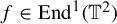 , the unstable bundle satisfies
$E^u(\tilde {x})=E^u(\tilde {a})$
 whenever
$a_0=x_0$
 , we say that f is a special endomorphism. We observe that being non-special is a
$C^1$
 open and
$C^r$
 dense condition (see [Reference Costa and MicenaCM22] for
$r=1$
 , and a local argument and [Reference HeHe17] for a general argument in the volume preserving case) among partially hyperbolic
$f\in \operatorname {End}^r({\mathbb {T}^2})$
 .
Given an ergodic f-invariant measure
$\mu $
 , we define its center exponent by

Notice that since the center bundle is deterministic, the above is well defined.
When f is non-special, the bundle
$E^u$
 does not integrate into an f-invariant foliation. Nevertheless, we can construct unstable manifolds using the natural extension (see §2.1): given an orbit
$\tilde {x}=\{x_i\}_{i\in {\mathbb Z}}$
 , one can apply the graph transform method along the sequence
$\{x_i\}_{i<0}$
 to construct an unstable manifold
${\mathcal W}^u(\tilde {x})$
 attached to the orbit
$\tilde {x}$
 (see [Reference Qian, Xie and ZhuQXZ09]). We say that an ergodic f-invariant probability measure
$\mu $
 is a u-Gibbs measure if the conditionals of
$\mu $
 along unstable manifolds are absolutely continuous with respect to the inner Lebesgue measure of the leaves (see §2.3).
Finally, we say that
$f\in \operatorname {End}^1({\mathbb {T}^2})$
 is strongly transitive if for every open set
$U\subset {\mathbb {T}^2}$
 , there exists an integer
$N>0$
 such that
$\bigcup _{n = 0}^{N}f^n(U)={\mathbb {T}^2}$
 . We can now state our main result.
Theorem 1.1. Let f be a
$C^2$
 partially hyperbolic strongly transitive endomorphism of
${\mathbb {T}^2}$
 . Let
$\mu $
 be an ergodic u-Gibbs measure of f with positive center exponent. Assume that f is not special and that
$\operatorname {supp}(\mu )={\mathbb {T}^2}$
 . Then,
$\mu $
 is the unique absolutely continuous invariant measure for f.
We do not know if a map f satisfying the assumptions of our main result is mostly expanding in the sense of [Reference Andersson and VásquezAV18], that is, if the existence of one fully supported u-Gibbs measure with positive center exponent would imply that every u-Gibbs measure have positive center exponent. We also do not know whether the results of [Reference Andersson and VásquezAV18] hold true in the non-invertible setting, although we believe that both answers are yes. Regardless, our result can be seen also as giving a new criteria for the existence and uniqueness of absolutely continuous invariant probability measures for partially hyperbolic endomorphisms in
${\mathbb {T}^2}$
 (see Corollary 1.2 below), going beyond the measure rigidity.
We also remark that one cannot drop the full support and transitivity assumptions simultaneously. Indeed, consider the product of
$f: \mathbb {S}^1 \to \mathbb {S}^1$
 a north pole–south pole diffeomorphism and
$g: \mathbb {S}^1 \to \mathbb {S}^1$
 a uniformly expanding map with stronger expansion than f. This system is partially hyperbolic, not transitive, and the Lebesgue measure on the circle
$\{N\} \times \mathbb {S}^1$
 given by
$\delta _N \times Leb_{\mathbb {S}^1}$
 has expanding center exponent and it is u-Gibbs. We can perturb this system to a non-special one which has the same features (as in §2.2.3), being also not transitive. This phenomenon cannot occur on the uniformly expanding case. Nonetheless, even a uniformly expanding (therefore strongly transitive) system can have u-Gibbs measures that do not have full support, as we explore in §1.2.
1.2 Some applications
The most important particular case of Theorem 1.1 concerns the case in which every unstable curve has a dense forward orbit. More precisely, we say that a partially hyperbolic element
$f\in \operatorname {End}^1({\mathbb {T}^2})$
 has dynamically minimal unstable leaves if, for every unstable manifold
$\gamma ={\mathcal W}^u(\tilde {x})$
 , one has
$\overline {\bigcup _{n\in {\mathbb N}}f^n(\gamma )}={\mathbb {T}^2}$
 . Given an ergodic, f-invariant u-Gibbs measure
$\mu $
 , for almost every (a.e.)
$x\in \operatorname {supp}(\mu )$
 , there exists at least one orbit
$\tilde {x}=\{x_i\}_{i\in {\mathbb Z}}$
 , with
$x_0=x$
 , so that the associated unstable manifold
${\mathcal W}^u(\tilde {x})$
 is contained in the support of
$\mu $
 . In particular, if f has dynamically minimal unstable leaves, then every u-Gibbs measure is fully supported. Therefore, we deduce from our main result the following corollary.
Corollary 1.2. Let
$f\in \operatorname {End}^2({\mathbb {T}^2})$
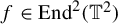 be partially hyperbolic, strongly transitive with dynamically minimal unstable leaves. Assume that f is non-special. Then, if there exists a u-Gibbs measure
$\mu $
 with positive center exponent, then
$\mu $
 is the unique absolutely continuous invariant measure of f.
This corollary reduces the measure rigidity problem of u-Gibbs measures with positive center exponent to the topological problem of proving dynamical minimality of unstable leaves.
1.2.1 Perturbations of an irreducible linear expanding map with simple spectrum
An interesting case in which Corollary 1.2 can be applied concerns perturbation of the induced map
$f_B:{\mathbb {T}^2}\to {\mathbb {T}^2}$
 , where
$B\in \operatorname {SL}_2({\mathbb Z})$
 has two irrational eigenvalues
$\sigma ^u>\sigma ^c>1$
 (see Example 2.13). This map is partially hyperbolic, strongly transitive, and special. In fact,
$f_B$
 is uniformly expanding in the sense that
$\min _{x\in {\mathbb {T}^2}}\|Df(x)|_{E^c}\|>1$
 . It is a well-known fact that this is an open condition which implies that every perturbation f of
$f_B$
 is topologically conjugate: there exists a continuous change of coordinates
$h\in \operatorname {Homeo}({\mathbb {T}^2})$
 under which f and
$f_B$
 are indistinguishable, that is,
$h\circ f=f_B\circ h$
 . A corollary of the work announced by [Reference Avila, Crovisier, Eskin, Potrie, Wilkinson and ZhangACE
+
24] is the following result.
Theorem 1.3. [Reference Avila, Crovisier, Eskin, Potrie, Wilkinson and ZhangACE + 24]
Consider
$f\in \operatorname {End}^2({\mathbb {T}^2})$
 a partially hyperbolic and uniformly expanding map which is topologically conjugate to
$f_B$
 . Then, f has dynamically minimal unstable leaves.
Remark 1.4. The above result can be proved using the s-transversality argument from [Reference Avila, Crovisier and WilkinsonACW25]. Indeed, a sketch of the proof goes as follows: if f is special, then by an argument from [Reference YuYu24], the conjugacy with
$f_B$
 preserves the unstable foliation and the minimality follows. If f is not special, then one shows that s-transversality always holds. This argument is called Rafael Potrie’s trick in a talk by Amie Wilkinson, available onlineFootnote
1
. Once s-transversality is established, [Reference Avila, Crovisier and WilkinsonACW25] shows that dynamical minimality must hold.
Combining this with Corollary 1.2, we obtain the following corollary.
Corollary 1.5. Let
$f\in \operatorname {End}^2({\mathbb {T}^2})$
 be a partially hyperbolic and uniformly expanding map which is topologically conjugate to
$f_B$
 . If f is not special, then f admits a unique u-Gibbs measure which is the unique absolutely continuous invariant measure.
In particular, this gives open sets of partially hyperbolic endomorphisms on
${\mathbb {T}^2}$
 displaying a unique u-Gibbs measure. Although this is a clean and direct application, we believe that the combination of the results and, most of all, the techniques developed in [Reference Avila, Crovisier, Eskin, Potrie, Wilkinson and ZhangACE
+
24] with Corollary 1.2 will have even more consequences, going beyond the uniformly expanding scenario. An evidence of this guess is that in the case of three-dimensional partially hyperbolic diffeomorphisms, some results giving uniqueness of u-Gibbs states will be given in [Reference Avila, Crovisier, Eskin, Potrie, Wilkinson and ZhangACE
+
24], notably in the smooth setting where [Reference KatzKat23] can be used.
1.2.2 The reducible case
Considering now a matrix
$A\in \operatorname {SL}_2({\mathbb Z})$
 with two distinct integer eigenvalues, both larger than
$1$
 , then the main obstruction to the application of our main result lies in the lack of knowledge about the behavior of unstable leaves. For in this case, a phenomenon not present in the invertible setting appears: the existence of compact unstable leaves. Indeed, we demonstrate in Example 2.15 that one can build a non-special perturbation of the induced map
$f_A$
 which presents compact unstable leaves with non-dense orbit. This example, despite being uniformly expanding, partially hyperbolic, strongly transitive, and not special, displays infinitely u-Gibbs measures. These claims are proved in §2.2.3.
More generally, we do not know what to expect as an answer to the following problem.
Problem 1.6. Let
$f\in \operatorname {End}^2({\mathbb {T}^2})$
 be a partially hyperbolic map isotopic to a linear expanding map
$f_A$
 , where the matrix A has integer eigenvalues
$\sigma ^u\geq \sigma ^c>1$
 . Do we have that every unstable curve is either compact or has a dense orbit?
Notice that the work of Martin Andersson and Wagner Ranter [Reference Andersson and RanterAR23] shows that, if we assume further than the assumptions of Problem 1.6 that

then f is locally eventually onto (for all
$U \subseteq M$
 non-empty open sets, there is
$N \in {\mathbb N}$
 such that
$f^N(U) = M$
 ) and, in particular, strongly transitive. Even under this stronger assumption, we do not know the answer to Problem 1.6.
1.3 An idea of the Eskin–Mirzakhani scheme
Let us give an overview of the argument we employ to prove Theorem 1.1. Consider a pair
$(f,\mu )$
 satisfying the assumptions of Theorem 1.1. First, one reduces the problem of demonstrating the absolute continuity of the measure to a very precise measure rigidity problem. In our setting, we do this by showing that the measure has the SRB property on the inverse limit space (see Definition 2.7). Since we are not in an homogeneous setting, we need to use normal form coordinates to linearize the dynamics along center unstable manifolds (see §3). This permits, among other things, to give a precise meaning to the statement that the u-Gibbs property is equivalent to ‘the measure is invariant by translations along unstable manifolds’. Thus, if we quotient the measure along unstable manifolds (see §3.3), we obtain a family of measures on the one-dimensional center manifolds, which by normal forms are mapped onto
${\mathbb R}$
 . Therefore, we obtain a family of measures
$\hat {\nu }^c_{\tilde {x}}$
 on the real line, attached to almost every point
$\tilde {x}$
 on the inverse limit, so that our u-Gibbs measure
$\mu $
 has the SRB property (and thus is absolutely continuous) if, and only if, the measures
$\hat {\nu }^c_{\tilde {x}}$
 are invariant by translations (Lemma 3.1). Moreover, this family inherits the starting invariance of our u-Gibbs measure
$\mu $
 : they (virtually) do not change when we move the base point
$\tilde {x}$
 to some
$\tilde {a} \in \widetilde {{\mathcal W}}^u(\tilde {x})$
 . Moreover, from x to
$f(x)$
 , the measure is multiplied by
$\|Df(x)|_{E^c}\|$
 (see Lemma 3.7 for a precise statement).
With proper adaptations, necessary in each context, this reduction of the measure rigidity problem to the problem of obtaining some kind of extra invariance along the direction of weak expansion is present in all previous works [Reference Alvarez, Leguil, Obata and SantiagoALOS24, Reference Benoist and QuintBQ11, Reference Brown and Rodriguez HertzBRH17, Reference Eskin and MirzakhaniEM18]. In this part of the proof, our contribution, comparing with [Reference Alvarez, Leguil, Obata and SantiagoALOS24, Reference KatzKat23], is to observe that it works also when one only assumes low regularity and non-uniform expansion along the center. Recall that the maps considered in [Reference Alvarez, Leguil, Obata and SantiagoALOS24] are Anosov and thus present uniform expansion along the center. Also, one can compare with [Reference KatzKat23] where the high smoothness is used from the start to obtain normal forms, in contrast to our work (and [Reference Alvarez, Leguil, Obata and SantiagoALOS24]) where we only need the map to be
$C^2$
 .
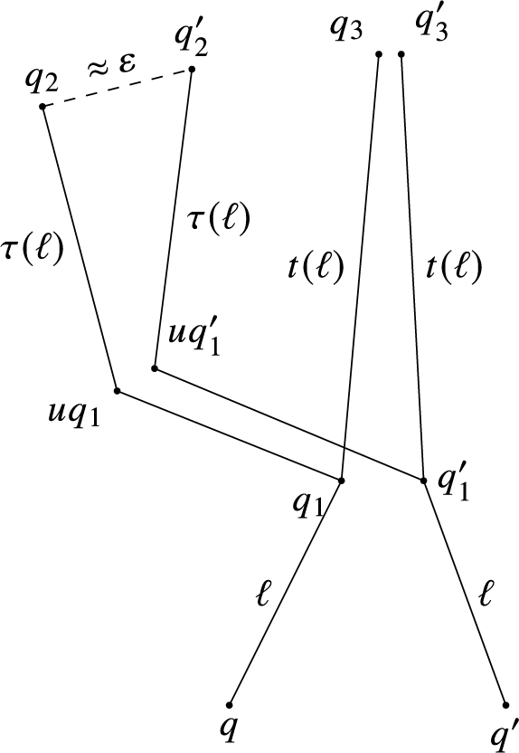
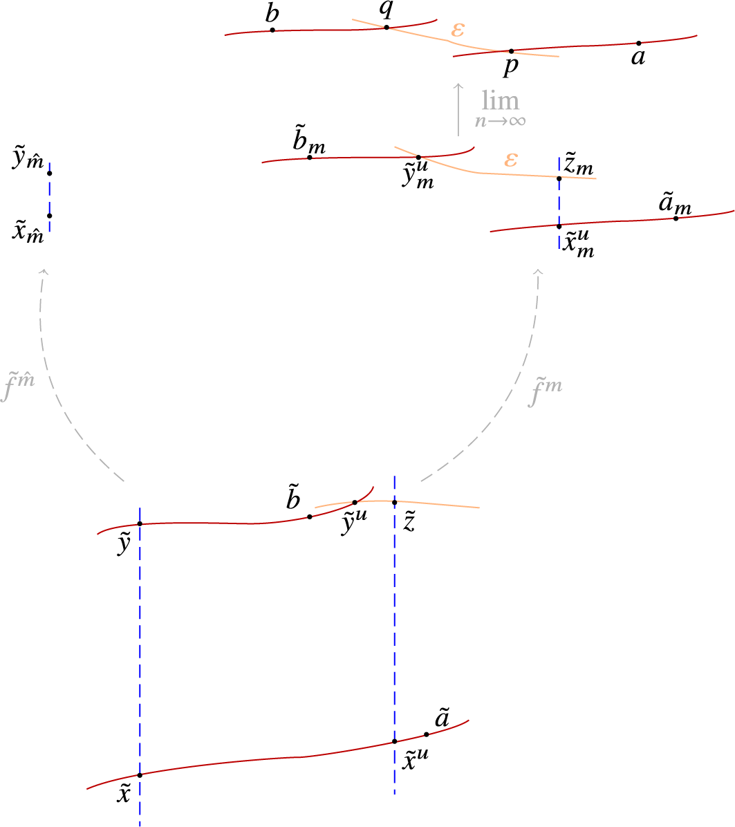
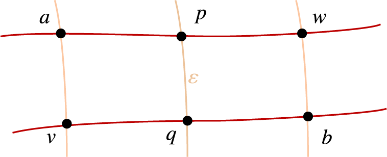
Once the reduction is completed, the factorization method of Eskin and Mirzakhani can roughly be described, following the scheme in Figure 1, as follows (see §7 where we implement the scheme in precise terms).
Illustration of Eskin–Mirzakhani scheme.

-
• On a ‘large set’, pick points q and $q'$
in the support of the measure such that q and
$q'$
are in the same stable leaf (which, in our case, means the fibers of the inverse limit space) with controlled distance. -
• The ‘randomness’ of the unstable direction along stable leaves ensures that $E^u(q)$
is uniformly transverse to
$E^u(q')$
. Thus, one has a uniform control on the center distance between q and
$q'$
. -
• Iterating forward by some time $\ell $
and moving to points
$uq_1\in \widetilde {{\mathcal W}}^u(q_1)$
and
${uq_1^{\prime }\in \widetilde {{\mathcal W}}^u(q^{\prime }_1)}$
(thus, ‘changing the future’), one gets an exponential estimate for the center distance between
$uq_1$
and
$uq_1^{\prime }$
of the form
$e^{-c\ell }$
for some
$c=c(q_1,q_1^{\prime },uq_1,uq_1^{\prime })>0$
. -
• Iterating forward by the new future for some time $\tau (\ell )$
, we find points
$q_2$
and
$q_2^{\prime }$
which are almost on the same center-unstable leaf and whose center distance is approximately
$\varepsilon $
. -
• Using the basic moves of quotient measures (see Lemma 3.7), one can find a time $t(\ell )$
so that the points
$q_3=f^{t(\ell )}(q_1)$
and
$q_3^{\prime }=f^{t(\ell )}(q_1^{\prime })$
satisfy $$ \begin{align*} \hat{\nu}^c_{q_2}\propto B_*\hat{\nu}^c_{q_3}\quad \text{and}\quad\hat{\nu}^c_{q_2^{\prime}}\propto \hat{B}_*\hat{\nu}^c_{q_3^{\prime}}, \end{align*} $$where B and $\hat {B}$
are linear maps of the real line with uniform slope (independent of
$\ell $
), and the notation
$\propto $
means that the measures are proportional (see §3.4). Indeed, notice that from
$uq_1$
to
$q_2$
, the measure changes by a linear factor of slope
$\|Df^{\tau (\ell )}(uq_1)|_{E^c}\|$
; thus, it suffices to find
$t=t(\ell )$
so that
$\|Df^t(q_1)|_{E^c}\|$
is almost of the same size than
$\|Df^{\tau (\ell )}(uq_1)|_{E^c}\|$
, and a similar procedure has to be done in the ‘
$q_1^{\prime }$
side’ of the picture.
-
• Since $q_3$
is exponentially close to
$q_3^{\prime }$
, if all points on the picture belong to a compact Lusin set where the family
$\hat {\nu }^c_{\tilde {x}}$
varies continuously, we deduce that $$ \begin{align*} \hat{\nu}^c_{q_2}\propto\widetilde{B}_*\hat{\nu}^c_{q_2^{\prime}}\quad\text{up to an error } \delta(\ell)\to_{\ell\to+\infty} 0, \end{align*} $$where $\widetilde {B}:{\mathbb R}\to {\mathbb R}$
is a linear map, with uniformly bounded slope.
-
• Thus, by taking limits, we find two points $q_{\infty }$
and
$q_{\infty }^{\prime }$
in the same center leaf, distant apart of approximately
$\varepsilon $
, so that their corresponding quotient measures change by a linear factor with uniformly bounded slope. This implies that
$\hat {\nu }^c_{q_{\infty }}$
has the necessary additional invariance (see Lemma 7.2).


In the last point of the argument, the fact that we have
$\dim E^c=1$
 plays a crucial role, since we need the affine structures given by normal forms. This is one of the key difficulties for generalizing our result to higher dimensions.
As in [Reference Alvarez, Leguil, Obata and SantiagoALOS24], we actually implement a modification of the above sketch where the points
$uq_1$
 and
$uq_1^{\prime }$
 are replaced by small unstable curves intersecting the good Lusin sets (see Lemma 6.4). Moreover, as we already pointed out, the main technical difference of our argument in comparison with [Reference Alvarez, Leguil, Obata and SantiagoALOS24] is that we work with non-uniform expansion along the center. This makes the matching argument (see [Reference Alvarez, Leguil, Obata and SantiagoALOS24, Proposition 11.8]) much more complicated, for we need to be extremely careful with several constants which are no longer uniform (depending only on f), but rather they are uniform on Lusin sets. For this reason, in Lemma 6.4, we work with two different Lusin sets. It is also worth remarking that our argument makes clearer the meaning of ‘factorization’ in our context: notice that the stopping times
$\tau (\ell )$
 and
$t(\ell )$
 depend on the exponential rate
$c=c(q_1,q_1^{\prime },uq_1,uq_1^{\prime })$
 . In our case, we can prove that, actually, c depends only on
$q_1$
 and thus, to have uniform estimations (like the synchronization of stopping times in Proposition 5.5), we only need that the points on the left side of the picture lie in a good Lusin set
${\mathcal L}_1$
 . This allows us to use
${\mathcal L}_1$
 to control the estimates and a larger set
${\mathcal L}_2\supset {\mathcal L}_1$
 to require continuity properties.
1.4 Structure of the paper
In §2, we introduce more comprehensively the dynamical systems with which we work: partially hyperbolic endomorphisms in dimension two. We also develop a number of important tools from Pesin theory, notably Lyapunov norms and distortion estimates. In §3, we discuss the generalization of the results from [Reference Alvarez, Leguil, Obata and SantiagoALOS24] on normal forms and the construction of quotient measures
$\hat {\nu }^c_{\tilde {x}}$
 to our setting. The proof of our main result starts at §4, where we give a different and simpler proof of the
$0-1$
 law of [Reference Alvarez, Leguil, Obata and SantiagoALOS24, Reference Brown and Rodriguez HertzBRH17], taking advantage of the symbolic structure of stable leaves. Sections 5 and 6 are devoted to the development of the concept of Y-configurations from [Reference Eskin and LindenstraussEL18, Reference Eskin and MirzakhaniEM18] (also used in [Reference Alvarez, Leguil, Obata and SantiagoALOS24, Reference KatzKat23]) in our setting. The main technical point of our argument (Lemma 6.4) is proved at the end of §6. Finally, in §7, we implement the Eskin–Mirzakhani scheme as in [Reference Alvarez, Leguil, Obata and SantiagoALOS24], using the conclusion of Lemma 6.4.
2 Partially hyperbolic endomorphisms on surfaces
In this section, we give complete definitions and state some properties of the kind of dynamical systems that we consider in this work. We present in detail the inverse limit space and how one can translate the theory of three-dimensional partially hyperbolic diffeomorphisms to the non-invertible setting. We present a number of examples and study their u-Gibbs measures. At the end, we develop the theory of Lyapunov norms in our setting, which is a convenient way of measuring the amount of expansion along the center direction. This tool plays a significant role in our argument.
2.1 Inverse limit
One of the key features of our work is to explore the connections between partially hyperbolic diffeomorphisms in dimension three, with a decomposition
$E^s\oplus E^c\oplus E^u$
 , and partially hyperbolic endomorphisms in dimension two. In this section, we describe the object which allows to properly formulate a dictionary between these classes of systems.
2.1.1 Abstract construction
Consider
$(X, d)$
 a compact metric space, and a map
${f: X \to X}$
 that is continuous and surjective. Then, f has an invertible extension
${\tilde {f}: X_f \to X_f}$
 , that is, there exists
$\pi : X_f \to X$
 continuous and surjective such that
$\pi \circ \tilde {f} = f \circ \pi $
 . This extension is called inverse limit or natural extension and it is defined as follows:
-
• $X_f = \{\tilde {x} = (x_k) \in X^{\mathbb {Z}}: x_{k+1} = f(x_k) { } \text { for all } k \in \mathbb {Z}\}$
; -
• $(\tilde {f}(\tilde {x}))_k = (x_{k+1}) \text { for all } k \in \mathbb {Z}$
and
$\text { for all } \tilde {x} \in \tilde {X}$
; -
• $\pi : X_f \to X$
is the projection on the zeroth coordinate.


Given
$\tilde {x},\tilde {y}\in X_f$
 , we define
$n(\tilde {x},\tilde {y}) \stackrel {\scriptscriptstyle \textrm { def.}}{=} \max \{n\in {\mathbb Z}\; : \; x_i=y_i\:\text {for all}\:|i|<n\}$
 . Then, by defining

we obtain a metric in
$X_f$
 which makes it a compact metric space.
Remark 2.1. The space
$(X_f,d)$
 is in fact an ultrametric space, in the sense that the improved triangle inequality holds:
$d(\tilde {x},\tilde {y})\leq \max \{d(\tilde {x},\tilde {z}),d(\tilde {z},\tilde {y})\}$
 for every
${\tilde {x},\tilde {y},\tilde {z}\in X_f}$
 .
Notice that the shift map
$\tilde {f}$
 and the projection
$\pi $
 are both continuous. If f is invertible, then
$\pi $
 is a homeomorphism between
$X_f$
 and X. We consider in this work only the case in which f is not invertible.
One can prove that the metric d generates the same topology as the open cylinders given by

where
$A_i \subseteq X$
 are open sets. The same cylinders generate the Borel
$\sigma $
 -algebra for
$(X_f, \tilde {d})$
 .
All measures considered in this work are over the Borel
$\sigma $
 -algebra for the given space and, given a space X, we denote by
${\mathcal M}(X)$
 the probability measures on X, endowed with the weak
$^*$
 topology. Given a discrete time dynamical system
$f:X\to X$
 , we denote by
${\mathcal M}_f(X)$
 the subset of f-invariant probability measures. Finally, we denote by
${\mathcal M}^{\operatorname {erg}}_f(X)$
 the ergodic elements in
${\mathcal M}_f(X)$
 .
It is easy to check that if
$\tilde {\mu }$
 is an
$\tilde {f}$
 -invariant measure on
$X_f$
 , then
$\pi _*\tilde {\mu }$
 is an f-invariant measure on X. Since
$\pi $
 is surjective, for all such
$\mu $
 , there is a
$\tilde {\mu }$
 that projects on it. Actually,
$\pi _*: \mathcal {M}_{\tilde {f}}(X_f) \to \mathcal {M}_f(X)$
 is a bijection, as proved for instance in [Reference Qian, Xie and ZhuQXZ09, Proposition I.3.1].
Proposition 2.2. Let
$(X,d)$
 be a compact metric space and
$f: X \to X$
 continuous. For any f-invariant probability measure
$\mu $
 on X, there is a unique
$\tilde {f}$
 -invariant probability measure
$\tilde {\mu }$
 on
$X_f$
 such that
$\pi _* \tilde {\mu } = \mu $
 .
The uniqueness on the above result is given by the fact that
$\tilde {\mu }$
 is defined by the values it attributes to cylinders.
The topological structure of
$(X_f, \tilde {d})$
 is quite interesting if f is not invertible. If X is connected and f is a self-covering map with positive degree, then, for each
$x \in X$
 ,
$\pi ^{-1}(x)$
 is compact, totally disconnected, and has no isolated points; thus, it is a Cantor set.
Remark 2.3. Additionally, if X is a manifold (it suffices that X is locally simply connected), then
$(X_f, X, \pi , \Sigma )$
 is a fiber bundle, where
$\Sigma $
 is a Cantor set [Reference Aoki and HiraideAH94, Theorem 6.5.1]. Therefore, even if X is a manifold and f is differentiable,
$X_f$
 does not have a manifold structure. Nevertheless, we can pullback the differential structure from X to
$X_f$
 and define
$D\tilde {f}_{\tilde {x}}: T_{\tilde {x}}X_f \to T_{\tilde {f}(\tilde {x})}X_f$
 as
$D\tilde {f}_{\tilde {x}} = Df_x$
 . This derivative is uniformly bounded as a function of
$\tilde {x}$
 . Using this tangent structure, we can see that each path connected component of
$X_f$
 is diffeomorphic to the universal covering of X, and that
$\tilde {f}$
 is invertible and as regular as f restricted to a given path connected component. Another topological feature of
$X_f$
 is given by the following result.
Notation 2.4. Herein, we use the notation

to refer to the fiber of
$\tilde {x}$
 on
$(X_f, X, \pi , \Sigma )$
 .
Proposition 2.5. For any f-invariant probability measure
$\mu $
 on X, we have
${\operatorname {supp}(\tilde {\mu })=X_f}$
 if and only if
$\operatorname {supp}(\mu )=X$
 .
Proof. If
$\operatorname {supp}(\tilde {\mu })=X_f$
 , then
$\operatorname {supp}(\mu )=X$
 is a direct consequence of
$\mu = \pi _* \tilde {\mu }$
 .
If
$\operatorname {supp}(\mu )=X$
 and we suppose that
$\operatorname {supp}(\tilde {\mu }) \neq X_f$
 , then there is an open set
$A \subseteq X_f$
 such that
$\tilde {\mu }(A) = 0$
 . Since
$\tilde {\mu }$
 is
$\tilde {f}$
 -invariant, this implies that
$\tilde {\mu }(\tilde {f}^k(A)) = 0$
 for all
$k \in \mathbb {Z}$
 . However, the topological structure of the inverse limit space implies that there is
$k < 0$
 such that
$\tilde {f}^k(A)$
 contains
$\pi ^{-1}(U)$
 for some open
$U \in X$
 , which is a contradiction.
2.1.2 Topological dynamics on
$X_f$

Recall that a continuous map
$f: X \to X$
 is said to be strongly transitive if for all
$U \subseteq X$
 non-empty open sets, there is
$N \in {\mathbb N}$
 such that
$\bigcup _{n=0}^N f^n(U) = X$
 . Every uniformly expanding map on a compact manifold is strongly transitive, and thus, it is transitive. The following simple result and its corollary are fundamental in allowing us to have ‘quantitative’ information about points which have ‘many’ different unstable directions (Lemma 4.3).
Lemma 2.6. Let
$f:X\to X$
 be a strongly transitive transformation. Then, for each
${x\in X}$
 , the set
$\{f^{-n}(x);n\in {\mathbb N}\}$
 is dense in X.
Proof. Let
$U\subset X$
 be any open set. Then, there exists
$N>0$
 such that
$\bigcup _{k=0}^N f^k(U)=X$
 . In particular, there exist some
$y\in U$
 and
$k \leq N$
 such that
$f^k(y)=x$
 , which means that
$f^{-k}(x)\cap U\neq \emptyset $
 .
Corollary 2.7. Let
$f:X\to X$
 be a strongly transitive transformation. Then, for each
$\tilde {x}\in X_f$
 , the set
$\{\tilde {f}^{-n}(\Sigma (\tilde {x}));n\in {\mathbb N}\}$
 is dense in
$X_f$
 .
2.2 Partial hyperbolicity on the inverse limit
Consider
$\operatorname {End}^r({\mathbb {T}^2})$
 the set of
$C^r$
 local diffeomorphisms on
${\mathbb {T}^2}$
 . Let
$f\in \operatorname {End}^1({\mathbb {T}^2})$
 be a partially hyperbolic endomorphism. We denote by
${\mathbb {T}_f^2}$
 the associated inverse limit space as constructed above. The cone field condition of partial hyperbolicity for f is equivalent to the following lemma [Reference Hirsch, Pugh and ShubHPS77, Reference Qian, Xie and ZhuQXZ09].
Lemma 2.8. There exists a continuous non-trivial splitting
$T_{\tilde {x}}{\mathbb {T}_f^2}=E^c(\tilde {x})\oplus E^u(\tilde {x})$
 on the inverse limit space for some choice of background Riemannian metric on
${\mathbb {T}^2}$
 , such that the continuous functions

satisfy the following inequalities:
-
(1) $\unicode{x3bb} ^c_{\tilde {x}}<\unicode{x3bb} ^u_{\tilde {x}}$
for every
$\tilde {x}\in {\mathbb {T}_f^2}$
; -
(2) $\unicode{x3bb} ^u_{\tilde {x}}>1$
for every
$\tilde {x}\in {\mathbb {T}_f^2}$
.


Notation 2.9. To simplify calculations involving derivatives along trajectories, we use the following notation:

and

for every
$n\in {\mathbb Z}$

Moreover, as a consequence of [Reference Costa and MicenaCM22], we have that the center bundle
$E^c$
 descends to an f-invariant bundle on
${\mathbb {T}^2}$
 .
Lemma 2.10. Let
$f\in \operatorname {End}^1({\mathbb {T}^2})$
 be partially hyperbolic. Then, for every
$\tilde {y}\in \Sigma (\tilde {x})$
 , one has
$E^c(\tilde {y})=E^c(\tilde {x})$
 .
Remark 2.11. In fact, if
$f: X \to X$
 is a local diffeomorphism with a
$Df$
 -invariant dominated splitting
$T_{\tilde {x}}X = E(\tilde {x}) \oplus F(\tilde {x})$
 , with
$E \prec F$
 , then
$E(x)$
 does not depend on
$\tilde {x} \in \pi ^{-1}(x)$
 . A proof of this fact for partially hyperbolic endomorphisms is given in [Reference Costa and MicenaCM22, Lemma 2.5].
The unstable bundle
$E^u$
 , however, in general, is not constant along fibers of the inverse limit space.
Definition 2.1. We say that a partially hyperbolic
$f\in \operatorname {End}^1({\mathbb {T}^2})$
 is special if for every
$\tilde {x}\in {\mathbb {T}_f^2}$
 and every
$\tilde {y}\in \Sigma (\tilde {x})$
 , one has
$E^u(\tilde {x})=E^u(\tilde {y})$
 .
2.2.1 Some examples
To get a more concrete view of the variety of behaviors one can encounter among partially hyperbolic elements
$f\in \operatorname {End}^1({\mathbb {T}^2})$
 , we discuss some simple examples.
Example 2.12. The simplest example is the reducible one given by the product of two expanding maps
$3x\ \pmod {1}$
 and
$2x\ \pmod {1}$
 in the circle
$\mathbb {S}^1 = {\mathbb R}/{\mathbb Z}$
 , the first expansion dominating the second one. Equivalently, consider
$f_A: \mathbb {T}^2 \to \mathbb {T}^2$
 as the transformation induced by the matrix
$A = (\begin {smallmatrix} 3 & 0\\ 0 & 2 \end {smallmatrix})$
 . This example is special, since it is linear, and each unstable/center leaf is a circle. It is worth remarking that it presents a behavior that is not present on invertible partially hyperbolic Anosov maps on the 3-torus, for in this case, the integer matrix A should have
$\vert \text {det}\ A \vert = 1$
 and the system is not reducible.
Example 2.13. Consider
$f_B: \mathbb {T}^2 \to \mathbb {T}^2$
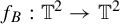 as the function induced by the matrix
$B = (\begin {smallmatrix} 3 & 1\\ 1 & 2 \end {smallmatrix})$
 , with eigenvalues
$({5+ \sqrt {5}}/{2})> ({5- \sqrt {5}}/{2}) > 1$
 . We have that
$f_B$
 is special and each unstable/center leaf is a dense line tangent to the corresponding eigenvector of B on the tangent space.
Both simple examples presented above are special. However, most partially hyperbolic endomorphisms are not special. More precisely, the set of non-special partially hyperbolic endomorphisms on a manifold X is
$C^1$
 open and dense [Reference Costa and MicenaCM22, Theorem B]. We remark that their result requires additional assumptions because they are considering systems with three non-trivial directions in the splitting and they are proving that both the center and the unstable directions are not unique for a given point. Nonetheless, the result holds, in particular, in dimension two as follows.
Theorem 2.14. [Reference Costa and MicenaCM22]
Consider
$PHE({\mathbb {T}^2})$
 as the set of all partially hyperbolic endomorphisms
$f: {\mathbb {T}^2} \to {\mathbb {T}^2}$
 with
$Df$
 -invariant splitting
$T_{\tilde {x}}M = E^c(x) \oplus E^u(\tilde {x})$
 . Then, there is a
$C^1$
 open and dense subset
$\mathcal {U} \subseteq PHE({\mathbb {T}^2})$
 such that every map in U is non-special.
The proof of denseness is achieved by, starting with a special partially hyperbolic endomorphism, perturbing it to generate new directions, as we do for completeness with the following example.
Example 2.15. Recall that
$f_A$
 from Example 2.12 is a special partially hyperbolic uniformly expanding endomorphism with the strong unstable direction
$E^u_A$
 being horizontal at every point, and the center direction
$E^c_A$
 being vertical at every point.
Consider
$p = (0, 0)$
 the unique fixed point of
$f_A$
 and
$q=(2/3,1/2) \in f_A^{-1}(\{p\})$
 . Since
$f_A$
 is a self-covering map, there is
$\tau> 0$
 such that, if
$f_A(y) = f_A(z)$
 and
$y \neq z$
 , then
$d(y,z)> \tau $
 . Take
$\delta \in (0, \tau /2)$
 and consider
$a \in \mathbb {R}$
 such that the square
${R = [-a,a]^2 \in \mathbb {R}^2}$
 , when projected under
$\exp _q: T_q{\mathbb {T}^2} \to {\mathbb {T}^2}$
 , is contained in
$B_{\delta }(q)$
 . Making an abuse of notation by identifying R and
$\exp _q(R)$
 , we define

where
$\varepsilon> 0$
 is as small as we want, and
$\psi _1: \mathbb {R} \to [-2,2]$
 and
$\psi _2: \mathbb {R} \to [0,1]$
 are
$C^\infty $
 functions satisfying:
-
• $\operatorname {supp} \psi _i \subseteq [-1,1]$
; -
• $\psi _1(1/2) = 1$
and
$\psi _1(-1/2) = -1$
; -
• $\psi _1(-1) = \psi _1(0) = \psi _1(1) = 0$
; -
• $\psi _1 |_{[-1/2,1/2]}$
is linear; -
• $\psi _2 |_{[-1/2,1/2]} \equiv 1$
.


We have that

in R, which is easily checked to be invertible for all
$(x,y)$
 , provided that
$\varepsilon $
 is sufficiently small.
Additionally,
$\varphi $
 is
$C^\infty $
 and satisfies
$\varphi (q) = q$
 ,
$\varphi |_{\overline {R^\complement }} = {\operatorname {Id}}$
 ,
$\varphi (R) = R$
 , and

meaning that
$\varphi $
 does not preserve the unstable directions of
$f_A$
 .
Let
$f\stackrel {\scriptscriptstyle \textrm {def.}}{=} f_A\circ \varphi $
 . Since f is
$C^1$
 close to
$f_A$
 , we have that f is a partially hyperbolic uniformly expanding endomorphism. Additionally, since
$(1,0)$
 is an eigenvector for
$D\varphi _{(x,y)}$
 , f has the same central manifolds as
$f_A$
 . The same argument as in [Reference Costa and MicenaCM22] gives us that f is non-special as follows.
By the definition of
$\delta $
 , we have that any point
$x\in {\mathbb {T}^2}$
 has a past orbit
$\tilde {x}\in \Sigma (x)$
 such that
$x_{-k}\notin R$
 for every
$k\in {\mathbb N}$
 . Thus, along this orbit, we have that
$f=f_A$
 , which implies that
$E^u(\tilde {x})=E^u_A$
 . In particular, there exists
$\tilde {q}\in \Sigma (q)$
 such that
$E^u(\tilde {q})$
 is horizontal. Now, by invariance, this implies that for
$\tilde {p}= \tilde {f}(\tilde {q}) = (\ldots q_{-1}q_0,p,p,p,\ldots )$
 , we have that

However, for
$\hat {p}=(\ldots p,p,p,\ldots )$
 , one has that
$f=f_A$
 all along this fixed orbit and thus
$E^u(\hat {p})=E^u_A$
 . This proves that p has more than one unstable direction and, thus, f is not u-special.
Similarly, we can do a perturbation of Example 2.13.
Example 2.16. We can repeat the construction from the previous example with
$q = ( \tfrac {2}{5}, \tfrac {4}{5} )$
 , and by using
$E^c_B(q)$
 and
$E^u_B(q)$
 as coordinates on
$T_q{\mathbb {T}^2}$
 to define
$\varphi $
 . Then, for all sufficiently small
$\varepsilon> 0$
 , there is a non-special partially hyperbolic uniformly expanding endomorphism g that is
$C^1$
 -close to
$f_B$
 from Example 2.13 and having the same center leaves.
2.2.2 Invariant foliations
Let
$f\in \operatorname {End}^r({\mathbb {T}^2})$
 be partially hyperbolic and let
${\tilde {f}:{\mathbb {T}_f^2}\to {\mathbb {T}_f^2}}$
 denote its lift to the inverse limit space. By viewing the direction of the fibers as a stable direction and the ‘manifold direction’ as a center-unstable direction, we can see the dynamics on the inverse limit space as partially hyperbolic as follows.
Definition 2.2. Given
$\tilde {x}\in {\mathbb {T}_f^2}$
 , we define its center-unstable manifold
$\widetilde {{\mathcal W}}^{cu}(\tilde {x})$
 as being the path-connected component of
${\mathbb {T}_f^2}$
 containing
$\tilde {x}$
 .
As we mentioned above, one can show that each center-unstable manifold
$\widetilde {{\mathcal W}}^{cu}(\tilde {x})$
 is homeomorphic to the universal cover
${\mathbb R}^2$
 of
${\mathbb {T}^2}$
 . Notice that
$\tilde {f}$
 acts permuting the components. Thus,
$\{\widetilde {{\mathcal W}}^{cu}(\tilde {x})\}_{\tilde {x}\in {\mathbb {T}_f^2}}$
 is an
$\tilde {f}$
 -invariant lamination of the space
${\mathbb {T}_f^2}$
 . This lamination is analogous to the center unstable foliation of a three-dimensional partially hyperbolic diffeomorphism. Indeed, notice that the fibers
$\Sigma (\tilde {x})$
 are contracted by the action of
$\tilde {f}$
 .
Remark 2.17. If
$\tilde {y}\in \Sigma (\tilde {x})$
 , then the definition of the metric in
${\mathbb {T}_f^2}$
 immediately implies
$d(\tilde {f}^n(\tilde {x}),\tilde {f}^n(\tilde {y}))\leq 2^{-n}$
 .
Thus, the fibers
$\Sigma $
 of the space
${\mathbb {T}_f^2}$
 play the same role as local stable manifolds in three-dimensional partially hyperbolic diffeomorphisms and they are ‘transverse’ to the center-unstable manifolds
$\widetilde {{\mathcal W}}^{cu}$
 . Clearly, there is a notorious difference, for here, the fibers are totally disconnected compact spaces and not embedded curves as in the case of diffeomorphisms.
Nonetheless, the graph transform method applies to the dynamics of
$\tilde {f}$
 on
${\mathbb {T}_f^2}$
 and one can show the following proposition (see [Reference Hirsch, Pugh and ShubHPS77, Reference Qian, Xie and ZhuQXZ09]).
Proposition 2.18. Given
$f\in \operatorname {End}^r({\mathbb {T}^2})$
 partially hyperbolic, there exists a one- dimensional unstable lamination
$\widetilde {{\mathcal W}}^u$
 of the space
${\mathbb {T}_f^2}$
 by
$\tilde {f}$
 -invariant immersed (on
$\widetilde {{\mathcal W}}^{cu}(\tilde {x})$
 )
$C^r$
 curves, varying continuously, which are everywhere tangent to
$E^u$
 .
The existence of a center foliation is a more delicate issue. In our setting, we have the following consequence of [Reference Hall and HammerlindlHH22, Theorem B].
Proposition 2.19. Let
$f\in \operatorname {End}^r({\mathbb {T}^2})$
 be a strongly transitive partially hyperbolic map. Then, there exists a one-dimensional (center) lamination
$\widetilde {{\mathcal W}}^c$
 of the space
${\mathbb {T}_f^2}$
 by
$C^r$
 immersed curves, varying continuously, which are everywhere tangent to
$E^c$
 . Moreover, this foliation descends to an f-invariant foliation of
${\mathbb {T}^2}$
 .
In this work, we use consistently the following notation:
$\widetilde {{\mathcal W}}^{*}(\tilde {x})$
 ,
$* \in \{u, c, cu \}$
 , is the leaf through the point
$\tilde {x}\in {\mathbb {T}_f^2}$
 , while
${\mathcal W}^{*}(\tilde {x})\stackrel {\scriptscriptstyle \textrm {def.}}{=}\pi (\widetilde {{\mathcal W}}^u(\tilde {x}))\subset {\mathbb {T}^2}$
 .
2.2.3 The unstable foliation of Example 2.15
The unstable foliation of Example 2.12 descends to a foliation by (horizontal) compact circles, while the center foliation is the foliation by vertical circles. In Example 2.15, as the map is not special, the unstable foliation on
${\mathbb {T}_f^2}$
 does not descend to a foliation of
${\mathbb {T}^2}$
 , while the center foliation remains the same as that of
$f_A$
 .
Moreover, we can choose the parameter
$a>0$
 small enough so that there exists some (meager) compact set
$K\subset \mathbb {S}^1$
 , which is forward invariant under
$x\mapsto 2x\mod 1$
 , and
$(\mathbb {S}^1\times K)\cap R=\emptyset $
 . Thus, after perturbation, the set
$\Gamma =\mathbb {S}^1\times K$
 remains invariant under the perturbed map f, as
$f=f_A$
 is restricted to
$\Gamma $
 . In particular, every horizontal unstable curve through a point
$x\in \Gamma $
 has non-dense forward orbit. Moreover, we have that there are points
$\tilde {x}\in {\mathbb {T}_f^2}$
 such that the set
$\bigcup _{i\in {\mathbb Z}}{\mathcal W}^u(x_i)$
 is not dense in
${\mathbb {T}^2}$
 . Indeed, for all
$x \in \Gamma $
 , there is
${\tilde {x}\in \Sigma (x)}$
 such that
$x_{-k}\in \Gamma $
 for every
$k\in {\mathbb N}$
 , which implies that
$E^u_f(\tilde {x}) = E^u_A$
 . Additionally, the uniform expansion of f allows us to make this choice of past orbit coherently along the compact curves in
$\Gamma $
 , in the sense that
${\mathcal W}^u(x_i) \subseteq \Gamma $
 for all
$i \leq 0$
 .
The behavior of the foliation in this example is still not well understood. We believe that every unstable curve which is not horizontal at some place should have a dense orbit, but this claim has not yet been confirmed.
2.3 u-Gibbs measures for endomorphisms
We are now able to define u-Gibbs measures on the non-invertible setting. Informally speaking, a u-Gibbs measure is a measure that is ‘well distributed’ with respect to an unstable foliation. Since, in general, there is no unstable foliation on the ambient manifold, the definition passes through the unstable leaves of the inverse limit.
To make this concept of a ‘well distributed’ measure with respect to a foliation precise, we first introduce how we decompose the measure with respect to a ‘nice partition’, with the following definition and theorem stated specifically for our context.
Let
$f\in \operatorname {End}^r({\mathbb {T}^2})$
 be a partially hyperbolic endomorphism.
Definition 2.3. A partition
$\mathcal {P}$
 of
${\mathbb {T}_f^2}$
 is a measurable (or countably generated) partition with respect to
$\tilde {\mu }$
 if there is
$M_0 \subseteq {\mathbb {T}_f^2}$
 with
$\tilde {\mu }(M_0) = 1$
 and a countable family
$\{A_i\}_{i \in {\mathbb N}}$
 of measurable sets such that, given
$P \in \mathcal {P}$
 , there is
$\{P_i\}_{i \in {\mathbb N}}$
 with
$P_i \in \{A_i, A_i^\complement \}$
 such that
$P = \bigcap \limits _{i \in {\mathbb N}} P_i$
 restricted to
$M_0$
 .
In other words, every element of the partition can be generated with the intersections of a countable family of measurable sets or their complements. For such partitions, the following result holds.
Theorem 2.20. (Rokhlin disintegration)
If
$\mathcal {P}$
 is a measurable partition for
${\mathbb {T}_f^2}$
 and
$\tilde {\mu }$
 , then
$\tilde {\mu }$
 has a disintegration on a family of conditional measures
$\{\tilde {\mu }_P\}_{P \in \mathcal {P}}$
 , that is, for all
$\phi : {\mathbb {T}_f^2} \to {\mathbb R}$
 continuous:
-
(1) $P \mapsto \int \phi \, d\tilde {\mu }_P$
is measurable; -
(2) $\tilde {\mu }_P(P) = 1$
for
$\hat {\mu }$
-a.e.
$P \in \mathcal {P}$
; -
(3) $\int \phi \, d\tilde {\mu } = \int _{\mathcal {P}} \int _P \phi \, d\tilde {\mu }_P\, d\hat {\mu } $
.


Here,
$\hat {\mu }$
 denotes the transverse measure given by
$\hat {\mu }(\mathcal {Q}) = (p_{\mathcal {P}})_*\mu (\mathcal {Q}) = \mu (p_{\mathcal {P}}^{-1}(\mathcal {Q}))$
 , where
$p_{\mathcal {P}}: {\mathbb {T}_f^2} \to \mathcal {P}$
 is the projection assigning for each point
$x \in {\mathbb {T}_f^2}$
 the element of
$\mathcal {P}$
 containing x.
Remark 2.21. The partition
$\{\Sigma (\tilde {x})\}_{\tilde {x}\in {\mathbb {T}_f^2}}$
 into fibers, being a decomposition of the space into a disjoint union of compact sets, is easily seen to be an example of a measurable partition. Given a probability measure
$\mu \in {\mathcal M}({\mathbb {T}^2})$
 , we denote by
$\{\mu _x\}_{x\in {\mathbb {T}^2}}$
 the conditional measures of its lift
$\tilde {\mu }$
 with respect to this partition.
A special case of measurable partition for which the above theorem applies is given by u-subordinate partitions.
Definition 2.4. A measurable partition
$\mathcal {P}$
 of
${\mathbb {T}_f^2}$
 is u-subordinate with respect to
$\mu $
 if, for
$\tilde {\mu }$
 -a.e.
$\tilde {x} \in {\mathbb {T}_f^2}$
 , the atom
$\mathcal {P}(\tilde {x})$
 satisfies:
-
(1) $\pi |_{\mathcal {P}(\tilde {x})}$
is a bijection onto its image; -
(2) there is a $C^1$
embedded submanifold
$U_{\tilde {x}} \subseteq {\mathbb {T}^2}$
with dimension equal to
$\dim E^u$
, such that
$U_{\tilde {x}} \subseteq {\mathcal W}^u(\tilde {x})$
,
$\pi (\mathcal {P}(\tilde {x})) \subseteq U_{\tilde {x}}$
, and
$\pi (\mathcal {P}(\tilde {x}))$
contains an open neighborhood of
$\pi (\tilde {x})$
in
$U_{\tilde {x}}$
.


The proof of the existence of u-subordinate partitions for non-invertible maps is given in [Reference Qian, Xie and ZhuQXZ09, §IX.2.2].
Definition 2.5. An f-invariant measure
$\mu $
 is said to be u-Gibbs if for every u-subordinate partition
$\mathcal {P}$
 for
$\mu $
 , we have

for
$\tilde {\mu }$
 -a.e.
$\tilde {x} \in {\mathbb {T}_f^2}$
 , where
$\{\tilde {\mu }^{\mathcal {P}}_{\tilde {x}}\}$
 is the disintegration of
$\tilde {\mu }$
 with respect to
$\mathcal {P}$
 and
$\text {Leb}^u_{\tilde {x}}$
 is the Lebesgue measure on
$U_{\tilde {x}}$
 .
Remark 2.22. Given
$\mu $
 a u-Gibbs measure, if
$\tilde {\mu }$
 is the unique lift to the inverse limit space, then it follows directly from the definition that
$\tilde {x} \in \operatorname {supp} \tilde {\mu }$
 implies
$\widetilde {{\mathcal W}}^u(\tilde {x}) \subseteq \operatorname {supp} \tilde {\mu }$
 . In other words, the support of
$\tilde {\mu }$
 is u-saturated.
2.3.1 u-Gibbs measures for the examples
Example 2.12 has many u-Gibbs measures: for any
$\nu $
 a (
$2x\ \pmod 1$
 )-invariant measure on
$\mathbb {S}^1$
 ,
$\operatorname {Leb}_{\mathbb {S}^1} \times \nu $
 is a u-Gibbs measure. Since the doubling map
$2x\ \pmod 1$
 is semi-conjugated to a full shift in two symbols, we know this system has infinitely many u-Gibbs measures. This is a particular case because the system is reducible.
In contrast, Example 2.13 has only
$\operatorname {Leb}_{\mathbb {T}^2}$
 as a u-Gibbs measure. A brief sketch of this argument goes as follows: up to a constant, the density of
$\tilde {\mu }$
 along some unstable leaf
$\widetilde {{\mathcal W}}^u(\tilde {x})$
 is given by

Since the map is linear, this shows that the density is constant and, thus, the conditional measure is invariant by translations along leaves. The invariance of conditional measures by translations along leaves implies invariance of the measure
$\mu $
 under the unity flow along leaves. However, the unity flow along leaves is a Diophantine flow, which is uniquely ergodic. One deduces that
$\mu =\text {Leb}_{{\mathbb {T}^2}}$
 .
Both Examples 2.12 and 2.13 are special, and one might wonder how the situation changes after perturbation. Example 2.15 gives us a non-special endomorphism, close to
$f_A$
 , which still has infinitely many u-Gibbs measures. Indeed, as we discussed above in §2.2.3, the example can be built with a forward invariant set
$\Gamma =\mathbb {S}^1\times K$
 which is made of horizontal compact unstable leaves. Moreover, K can be chosen so that it contains infinitely many
$x\mapsto 2x\mod 1$
 periodic orbits. Given
$x_1,\ldots ,x_k$
 such periodic orbits, the measure

is a u-Gibbs measure for f.
However, Example 2.16 is also non-special, but since we can apply Corollary 1.2, we deduce that the map has only one u-Gibbs measure which is the unique absolutely continuous invariant measure.
2.3.2 Uniform density estimate
For a Lebesgue measurable set
$A\subset \widetilde {{\mathcal W}}^u(\tilde {x})$
 , we denote, for simplicity,
$|A|\stackrel {\scriptscriptstyle \textrm {def.}}{=}\text {Leb}^u_{\tilde {x}}(A)$
 the Lebesgue measure of A. Given a u-Gibbs measure, the conditional measures are ‘comparable’ with respect to Lebesgue, but only up to a measurable function. To be precise, the density
$({\tilde {\mu }_{\tilde {x}}}/{\text {Leb}^u_{\tilde {x}}})$
 is a measurable function. By restricting to compact sets of large measure, we get a uniform comparison, as made clear by the next result.
Lemma 2.23. Let
$f\in \operatorname {End}^r({\mathbb {T}^2})$
 be partially hyperbolic and
$\mu $
 be an ergodic u-Gibbs measure for f. Consider
$\{\tilde {\mu }^u_{\tilde {x}}\}$
 a family of conditional measures with respect to a u-subordinate partition. Then, given
$\delta>0$
 , there exists a compact Lusin set
${\mathcal L}\subset {\mathbb {T}_f^2}$
 , with
$\tilde {\mu }({\mathcal L})>1-\delta $
 , for which there exists a constant
$C=C({\mathcal L})$
 such that for every subset
$A\subset \widetilde {{\mathcal W}}^u_1(\tilde {x})$
 , for
$\tilde {x}\in {\mathcal L}$
 , one has
$C^{-1}|A|\leq \tilde {\mu }^u_{\tilde {x}}(A)\leq C|A|$
 .
Proof. From the definition of u-Gibbs measure, it follows that for
$\tilde {\mu }$
 -a.e.
$\tilde {x}\in {\mathbb {T}_f^2}$
 , there exists a density function
$\rho ^u_{\tilde {x}}$
 such that

Moreover, up to a positive constant depending measurably on
$\tilde {x}$
 , we have that the density
$\rho ^u_{\tilde {x}}(t)$
 ,
$t=\pi (\tilde {y})$
 , is given by

By Lusin’s theorem, given
$\delta>0$
 , there exists a compact set
${\mathcal L}$
 with measure
$\tilde {\mu }({\mathcal L})>1-\delta $
 such that the assignment
$\tilde {x}\in {\mathcal L}\mapsto \rho ^u_{\tilde {x}}$
 is continuous. In particular, there exists a constant C such that
$ C\geq \rho ^u_{\tilde {x}}(t)\geq C^{-1}$
 for every
$\tilde {x}\in {\mathcal L}$
 and every
$t=\pi (\tilde {y})$
 , where
$\tilde {y}$
 belongs to the atom containing
$\tilde {x}$
 .
Notation 2.24. Since uniform estimates such as the one above are abundant in this paper, we use repeatedly the following notation: given
$a,b,C>0$
 , we say that
$a\asymp _Cb$
 provided that
$C^{-1}b\leq a\leq Cb$
 .
2.4 Pesin theory in the partially hyperbolic setting
In this section, we consider
${f:{\mathbb {T}^2}\to {\mathbb {T}^2}}$
 a partially hyperbolic endomorphism and
$\mu \in {\mathcal M}_f^{\operatorname {erg}}({\mathbb {T}^2})$
 an ergodic invariant probability measure.
2.4.1 Center Lyapunov exponent
The (pointwise) center Lyapunov exponent of f is defined for all points in the f-invariant regular set
$\Gamma $
 , where
$\Gamma $
 has full
$\mu $
 -measure for any f-invariant measure
$\mu $
 . It is given by

The integrated center Lyapunov exponent with respect to
$\mu $
 is given by

using the fact that
$E^c$
 is one-dimensional and Birkhoff ergodic theorem. Since
$L^c(x)$
 is f-invariant and since we work only with ergodic measures, then
$L^c(x) = L^c(\mu )$
 for
$\mu $
 -almost every point and non-uniform expansion is given by
$L^c(x)> 0$
 for
$\mu $
 -almost every point.
The differential structure of f pulled back to
${\mathbb {T}_f^2}$
 allows us to have an Oseledec’s theorem for the inverse limit space, and the Lyapunov exponents are the same as in the original manifold and they do not depend on the past orbit, that is, they are constant along
$\Sigma (\tilde {x})$
 , see [Reference Qian, Xie and ZhuQXZ09, Proposition I.3.5]. In §2.4, we explore Pesin theory further.
From now on, we consider a fixed ergodic f-invariant measure
$\mu $
 . We also assume that the center Lyapunov exponent of
$\mu $
 satisfies
$L^c(\mu )>0$
 . In this setting, we fix
$0<\unicode{x3bb} <L^c(\mu )<\hat {\unicode{x3bb} }$
 . Then, there exists a measurable function
$C:{\mathbb {T}_f^2}\to [1,+\infty )$
 such that

for every
$n>0$
 and

for every
$n<0$
 . Moreover, the function C has slow exponential growth:

where
$\varepsilon =(\hat {\unicode{x3bb} }-\unicode{x3bb} )/2$
 .
2.4.2 Pesin center manifolds
We now briefly recall the properties of the Pesin center manifolds in our setting. There exists a pair of measurable functions
$r:{\mathbb {T}_f^2}\to (0,1)$
 and
$\gamma :{\mathbb {T}_f^2}\to [1,+\infty )$
 such that whenever
$\tilde {y},\tilde {z}\in \widetilde {{\mathcal W}}^c_{r(\tilde {x})}(\tilde {x})$
 , then

Notation 2.25. We use the notation
$\widetilde {{\mathcal W}}^c$
 for the global center manifold given by the partially hyperbolic splitting and
$\widetilde W^c_{{\operatorname {loc}}}$
 for the Pesin manifolds where we observe expansion, which in this case are local manifolds contained on
$\widetilde {{\mathcal W}}^c$
 for almost every point, that is,
$\widetilde W^c_{\operatorname {loc}}(\tilde {x})=\widetilde {{\mathcal W}}^c_{r(\tilde {x})}(\tilde {x})$
 .
The global Pesin manifolds, which we denote by
$\widetilde W^c(\tilde {x})$
 , are defined by the classical formula

Thus,
$\widetilde W^c(\tilde {x})\subseteq \widetilde {{\mathcal W}}^c(\tilde {x})\subset \widetilde {{\mathcal W}}^{cu}(\tilde {x})$
 is an immersed line. As a priori, we assume no uniform expansion along
$E^c$
 , the inclusion
$\widetilde W^c(\tilde {x})\subseteq \widetilde {{\mathcal W}}^c(\tilde {x})$
 could be strict. We define the global Pesin center unstable manifolds by

As in [Reference Alvarez, Leguil, Obata and SantiagoALOS24, Lemma 2.4], we have the following lemma.
Lemma 2.26. For every
$\tilde {y}\in \widetilde W^c(\tilde {x})$
 , it holds that
$\widetilde W^c(\tilde {x})\cap \widetilde {{\mathcal W}}^u(\tilde {y})=\{\tilde {y}\}$
 .
2.4.3 The SRB property
Consider now a measurable partition
${\mathcal P}^{cu}$
 subordinate to the Pesin center unstable foliation
$\widetilde W^{cu}(\tilde {x})$
 . This means a measurable partition whose atoms are entirely contained in a Pesin center-unstable manifold and project bijectively onto measurable subsets of
${\mathbb {T}^2}$
 which contain a ball. More precisely, we give the following definition.
Definition 2.6. A measurable partition
$\mathcal {P}$
 of
${\mathbb {T}_f^2}$
 is cu-subordinate with respect to
$\mu $
 if, for
$\tilde {\mu }$
 -a.e.
$\tilde {x} \in {\mathbb {T}_f^2}$
 , the atom
$\mathcal {P}(\tilde {x})$
 satisfies:
-
(1) $\pi |_{\mathcal {P}(\tilde {x})}$
is a bijection onto its image; -
(2) there is an open set $U_{\tilde {x}} \subseteq {\mathbb {T}^2}$
such that
$\pi (\mathcal {P}(\tilde {x}))\supseteq U_{\tilde {x}}$
.


The construction of subordinate partitions in [Reference Ledrappier and StrelcynLS82] applies in our case.
Definition 2.7. We say that
$\mu $
 is an SRB measure if there exists a cu-subordinate partition
${\mathcal P}$
 such that for
$\tilde {\mu }$
 -a.e.
$\tilde {x}$
 , one has
$\pi _{*}\tilde {\mu }^{{\mathcal P}}_{\tilde {x}}<<\text {Leb}_{{\mathbb {T}^2}}$
 .
Lemma 2.27. Every SRB measure is absolutely continuous with respect to
$\text {Leb}_{{\mathbb {T}^2}}$
 .
Proof. Let us assume by contradiction that
$\mu $
 is not absolutely continuous with respect to
$\text {Leb}_{{\mathbb {T}^2}}$
 . Then, there exists a Borel measurable set
$A\subset {\mathbb {T}^2}$
 with
$\mu (A)>0$
 , but
${\text {Leb}_{{\mathbb {T}^2}}(A)=0}$
 . Then,
$\widetilde {A}\stackrel {\scriptscriptstyle \textrm { def.}}{=}\pi ^{-1}(A)$
 satisfies
$\tilde {\mu }(\widetilde {A})>0$
 . By the regularity of
$\mu $
 , we may assume that A is compact and contained in an open set
$U=B_r(x)$
 for some
$x\in A$
 , such that
$\pi |_{\pi ^{-1}(U)\cap \widetilde {{\mathcal W}}^{cu}(\tilde {y})}$
 is a bijection for every
$\tilde {y}\in \pi ^{-1}(x)$
 . We may also choose the point x so that for
$\mu _x$
 -a.e.
$\tilde {y}\in \pi ^{-1}(x)$
 , the measure
$\pi _*\tilde {\mu }^{{\mathcal P}}_{\tilde {y}}$
 is absolutely continuous with respect to
$\text {Leb}_{{\mathbb {T}^2}}$
 . In particular, we have that

for
$\mu _x$
 -a.e.
$\tilde {y}\in \pi ^{-1}(x)$
 . However, this implies that

which gives a contradiction.
2.4.4 Distortion estimates
Given
$\delta>0$
 , we can choose a compact set
${\mathcal L}\subset {\mathbb {T}_f^2}$
 with
$\tilde {\mu }({\mathcal L})>1-\delta $
 and such that the functions
$C,r,\gamma $
 are continuous when restricted to
${\mathcal L}$
 . For this section, we fix
$\delta>0$
 and
${\mathcal L}$
 .
The following result is a classical consequence of uniform expansion along unstable manifolds or center Pesin manifolds.
Lemma 2.28. Let
$\varphi : {\mathbb {T}_f^2} \to {\mathbb R}$
 be a Hölder continuous function. There exists constants
$C_0>0$
 and
$C=C({\mathcal L})>0$
 such that:
-
(1) if $\tilde {y} \in \widetilde {{\mathcal W}}^u_1(\tilde {x})$
, then for every
$n>0$
, $$ \begin{align*} \bigg\vert\! \sum_{l=0}^{n-1} \varphi(\tilde{f}^{-l}(\tilde{x})) - \varphi(\tilde{f}^{-l}(\tilde{y})) \bigg\vert \leq C_0; \end{align*} $$
-
(2) if $\tilde {f}^{l}(\tilde {y}) \in \widetilde {{\mathcal W}}^u_{1}(\tilde {f}^{l}(\tilde {x}))$
for
$l \in \{0, \ldots , n-1 \}$
, then $$ \begin{align*} \bigg\vert\! \sum_{l=0}^{n-1} \varphi(\tilde{f}^l(\tilde{x})) - \varphi(\tilde{f}^l(\tilde{y})) \bigg\vert \leq C_0; \end{align*} $$
-
(3) if $\tilde {y} \in \widetilde W^c_{r(\tilde {x})}(\tilde {x})$
and
$\tilde {x} \in {\mathcal L}$
, then for every
$n> 0$
, $$ \begin{align*} \bigg\vert\! \sum_{l=0}^{n-1} \varphi(\tilde{f}^{-l}(\tilde{x})) - \varphi(\tilde{f}^{-l}(\tilde{y})) \bigg\vert \leq C; \end{align*} $$
-
(4) if $\tilde {f}^{l}(\tilde {y}) \in \widetilde W^c_{r(\tilde {f}^{l}(\tilde {x}))}(\tilde {f}^{l}(\tilde {x}))$
for
$l \in \{0, \ldots , n-1 \}$
and
$\tilde {f}^{n}(\tilde {x}) \in {\mathcal L}$
, then $$ \begin{align*} \bigg\vert\! \sum_{l=0}^{n-1} \varphi(\tilde{f}^l(\tilde{x})) - \varphi(\tilde{f}^l(\tilde{y})) \bigg\vert \leq C. \end{align*} $$





Proof. We write the proof for condition (2) and the center leaf, the others being analogous. If
$\tilde {x} \in {\mathcal L}$
 and
$\tilde {y} \in \widetilde W^c_{r(\tilde {x})}(\tilde {x})$
 , then

for all
$n \in \mathbb {N}$
 , where
$\gamma _0=\max \gamma |_{{\mathcal L}}$
 .
We have that

where
$\varphi $
 is
$\alpha $
 -Hölder with constant K. This is less or equal to

We immediately have the following result.
Lemma 2.29. There exists a constant
$C=C(f)>1$
 such that if
$\tilde {f}^n(\tilde {y})\in {\mathcal W}^u_{1}(\tilde {f}^n(\tilde {x}))$
 , then for every
$\ell \leq n$
 ,

Also, as a direct consequence of our choice of
$\mathcal {L}$
 , we have similar estimates for the center direction.
Lemma 2.30. Given a Lusin set
${\mathcal L}$
 , there exists a constant
$C=C({\mathcal L})>1$
 such that if
$\tilde {f}^n(\tilde {x})\in {\mathcal L}$
 and
$\tilde {f}^n(\tilde {y})\in \widetilde W^c_{r(\tilde {f}^n(\tilde {x}))}(\tilde {f}^n(\tilde {x}))$
 , then for every
$\ell \leq n$
 ,

2.5 The Lyapunov norm
Given
$v\in E^c(\tilde {x})\setminus \{0\}$
 and
$0< \unicode{x3bb} < L^c(\mu )$
 , we define

which is called the Lyapunov norm of v. Observe that all terms in the series are non-negative, but, in principle, the series could diverge. The following lemma guarantees that this is not the case by providing a measurable upper bound with respect to the background Riemannian norm.
Lemma 2.31. There exists a measurable function
$\xi :{\mathbb {T}_f^2}\to [1,+\infty )$
 such that for
$\tilde {\mu }$
 -a.e.
$\tilde {x}\in {\mathbb {T}_f^2}$
 and every
$v\in E^c(\tilde {x})$
 , it holds that
$\|v\|\leq \|v\|_{L,\tilde {x}}\leq \xi (\tilde {x})\|v\|$
 .
Proof. Denote, for simplicity,
$\chi \stackrel {\scriptscriptstyle \textrm {def.}}{=} L^c(\mu )$
 . Choose
$0<\varepsilon <\chi -\unicode{x3bb} $
 . Then, there exists a measurable function
$\hat {C}:{\mathbb {T}_f^2}\to [1,+\infty )$
 such that

This implies that

Thus, defining
$\xi (\tilde {x})\stackrel {\scriptscriptstyle \textrm {def.}}{=} (\hat {C}(\tilde {x})^{-2}\sum _{k\leq 0}e^{2k(\chi -\varepsilon -\unicode{x3bb} )})^{1/2}$
 , we obtain

2.5.1 Growth estimate for norm
$\|.\|_{L,\tilde {x}}$

When we measure the length of a vector
${v\in E^c(\tilde {x})}$
 using the norm
$\|.\|_{L,\tilde {x}}$
 , we see expansion in a uniform fashion. The drawback is that the assignment
$x\mapsto \|.\|_{L,\tilde {x}}$
 is only measurable. In the following, we use the notation
$\tilde {x}_n=\tilde {f}^n(\tilde {x})$
 .
Lemma 2.32. There exists a constant
$\sigma =\sigma (f)>1$
 such that for
$\tilde {\mu }$
 -a.e.
$\tilde {x}\in {\mathbb {T}_f^2}$
 and every
$v\in E^c(\tilde {x})$
 , it holds that

Proof. Take
$v\in E^c(\tilde {x})\setminus \{0\}$
 and
$n>0$
 . Then,

By making the change
$\ell \rightarrow k+n$
 in the sum, we obtain

Term I is equal to

As term II is non-negative, this gives immediately the lower bound. For the upper bound, take
$\xi>\max \{\log \|D\tilde {f}(\tilde {x})\|;\tilde {x}\in {\mathbb {T}_f^2}\}>1$
 . Notice that
$n<e^{n\xi }$
 for every
$n>0$
 . By definition, for every
$\ell =1,\ldots ,n$
 , we have

This allows us to estimate term II above by

Thus,

This establishes the upper bound and completes the proof.
2.5.2
u-saturation of the well-behaved set for
$\|.\|_{L,\tilde {x}}$

Lemma 2.33. If
$\tilde {x}$
 is
$\tilde {\mu }$
 -regular and if
$\tilde {x}^u\in \tilde {{\mathcal W}}^u(\tilde {x})$
 , then
$0<\|v\|_{L,\tilde {x}^u}<+\infty $
 for every
$v\in E^c(\tilde {x}^u)$
 . The same holds for every
$\tilde {y}\in \widetilde W^c_{r(\tilde {x})}(\tilde {x})$
 .
Proof. As
$\tilde {x}\mapsto \log \|D\tilde {f}(\tilde {x})|_{E^c}\|$
 is Hölder continuous, it follows from Lemma 2.28 that

for some constant
$C>1$
 (which depends only on f and
$d(\tilde {x},\tilde {x}^u)$
 ). Since
$E^c$
 is one-dimensional, we can therefore write

which implies the result. The proof for
$\tilde {y}\in \widetilde {{\mathcal W}}^c_{r(\tilde {x})}(\tilde {x})$
 is identical. Indeed, the argument for the distortion Lemma 2.28 shows that

for every
$n>0$
 , where
$C=C(\tilde {x})>1$
 . It follows as before that
$\|v\|^2_{L,\tilde {y}}\asymp _{C^2}\|v\|_{L,\tilde {x}}^2$
 .
2.5.3 Distortion estimates
We consider now a Lusin set
${\mathcal L}\subset {\mathbb {T}_f^2}$
 of measure
$\tilde {\mu }({\mathcal L})>1-\delta $
 .
Notation 2.34. Given
$\tilde {x}\in {\mathbb {T}_f^2}$
 and
$n\in {\mathbb N}$
 , we define
$\hat {\unicode{x3bb} }^c_{\tilde {x}}(n) \stackrel {\scriptscriptstyle \textrm {def.}}{=} ({\|D\tilde {f}^n(\tilde {x})v\|_{L,\tilde {x}_n}})/({\|v\|_{L,\tilde {x}}})$
 for
$v\in E^c(\tilde {x})\setminus \{0\}$
 . It is easy to check that

Remark 2.35. Observe from Lemma 2.32, the following estimate:

for every
$n\in {\mathbb Z}$
 and for a constant
$0<\unicode{x3bb} <L^c(\mu )$
 , which is fixed, and for
$\sigma =\sigma (f)$
 , the constant given in Lemma 2.32. This estimation only reflects the fact that when measuring growth with the Lyapunov norm, we see immediate expansion along
$E^c$
 . This will be of crucial importance later when we establish our quasi-isometric and synchronization estimates for stopping times.
We begin with a distortion result along Pesin center manifolds.
Lemma 2.36. There exists a constant
$C=C({\mathcal L})>1$
 such that, given
$n>0$
 , if
$\tilde {x}_n\in {\mathcal L}$
 and
$\tilde {y}_n\in \widetilde W^c_{r(\tilde {x})}(\tilde {x}_n)$
 , then

Proof. Notice that we are under the same assumptions of Lemma 2.30. Let
$C=C({\mathcal L})$
 be the constant given by that lemma. Then, given any non-zero vector
$v\in E^c(\tilde {x})$
 , we have that

The proof of Lemma 2.33 shows that
$\|v\|_{L,\tilde {y}}/\|v\|_{L,\tilde {x}}\asymp _{C} 1$
 . We deduce that

which gives the desired result.
We turn now to the case of two points on the same fiber of
${\mathbb {T}_f^2}$
 . In this case, we need to assume that both points belong to the Lusin set. Indeed, for the next lemma, we demand another property of the Lusin set.
Lemma 2.37. Given a Lusin set
${\mathcal L}\subset {\mathbb {T}_f^2}$
 there exists a constant
$C=C({\mathcal L})>1$
 such that whenever
$\tilde {x},\tilde {y}\in {\mathcal L}$
 with
$\tilde {y}\in \Sigma (\tilde {x})$
 , we have that

Proof. The function
$\xi $
 of Lemma 2.31 is uniformly bounded in
${\mathcal L}$
 . Also, given any tangent vector
$v\in E^c(\tilde {x})$
 , there exists a unique (up to orientation) vector
$\hat {v}\in E^c(\tilde {y})$
 such that
$\|v\|=\|\hat {v}\|$
 .
Now, write as in the proof of Lemma 2.32 that

for all
$v\in E^c(\tilde {x})$
 and for all
$n>0$
 . Obviously, the same formula holds with
$\tilde {x}$
 and v replaced by
$\tilde {y}$
 and
$\hat {v}$
 . Since
$\tilde {x},\tilde {y}\in {\mathcal L}$
 , we have that

The basic distortion lemma gives that
$\|D\tilde {f}^j(\tilde {x})v\|\asymp _C\|D\tilde {f}^j(\tilde {y})\hat {v}\|$
 . Up to enlarging the constant C, we get
$\|D\tilde {f}^n(\tilde {x})v\|_{L,\tilde {x}}\asymp _C\|D\tilde {f}^n(\tilde {y})\hat {v}\|_{L,\tilde {y}}$
 . Therefore, up to enlarging C once more, we have

The following distortion result concerns points in the same unstable dynamical ball. The proof follows from the same calculations we have done in this section, so we refrain from repeating the details.
Lemma 2.38. There exists a constant
$C=C(f)>1$
 depending only on f such that for every
$\tilde {\mu }$
 generic point
$\tilde {x}\in {\mathbb {T}_f^2}$
 and every
$\tilde {a}\in \widetilde {{\mathcal W}}^u_1(\tilde {x})$
 , if
$\tilde {a}_n\in \widetilde {{\mathcal W}}^u_1(\tilde {x}_n)$
 for some
$n\in {\mathbb N}$
 , then

3 Normal forms and leaf-wise quotient measures
This section collects a number of tools we use in our argument. To motivate these tools, recall that our goal is to prove that, under the hypotheses of Theorem 1.1, a given u-Gibbs measure is absolutely continuous with respect to
$\operatorname {Leb}_{{\mathbb {T}^2}}$
 . Since, by definition, a u-Gibbs measure is (in some sense) homogeneous along unstable leaves, we claim that it is enough to show that the measure is also homogeneous along center leaves. This claim is made precise by the following result, which we prove in §3.3.
Lemma 3.1. There is a family of locally finite Radon measures
$\{\hat {\nu }^c_{\tilde {x}}\}_{\tilde {x} \in \mathbb {T}^2_f}$
 on
$\mathbb {R}$
 such that, if
$\hat {\nu }^c_{\tilde {x}}$
 is equivalent to Lebesgue for
$\tilde {\mu }$
 -a.e.
$\tilde {x}$
 , then
$\mu $
 is absolutely continuous with respect to Lebesgue.
This essentially translates our main problem into a one-dimensional question and it is the main goal of this section. To prove this lemma, we introduce a crucial tool: normal forms.
All the arguments in this section follow closely [Reference Alvarez, Leguil, Obata and SantiagoALOS24, §§6–7], so we only give a brief account for the sake of completeness.
3.1 One-dimensional normal forms
The result below, which comes from [Reference Kalinin and KatokKK07], provides us with invariant affine structures along Pesin center manifolds and unstable manifolds.
Proposition 3.2. For
$\tilde {\mu }$
 -almost every point
$\tilde {x}\in \mathbb {T}^2_f$
 , there are diffeomorphisms
$\mathcal {R}^u_{\tilde {x}}: \widetilde {{\mathcal W}}^u(\tilde {x}) \to {\mathbb R}$
 and
${\mathcal R}^c_{\tilde {x}}:\widetilde W^c(\tilde {x})\to {\mathbb R}$
 , which are both as regular as f, such that we have the following.
-
(1) Given $\tilde {x}$
and
$v\in E^*(\tilde {x})$
a unity vector, one has
$R^*_{\tilde {x}}(\tilde {x})=0$
and
$DR^*_{\tilde {x}}(\tilde {x})v=1$
. -
(2) Let $\Lambda ^{*}_{\tilde {x}}:{\mathbb R}\to {\mathbb R}$
denote the linear map
$\Lambda ^{*}_{\tilde {x}}(t)=\unicode{x3bb} ^{*}_{\tilde {x}}t$
. Considering
$\Phi ^{*}_{\tilde {x}}=(\mathcal {R}^{*}_{\tilde {x}})^{-1}$
, we have $$ \begin{align*} \mathcal{R}^{*}_{\tilde{f}(\tilde{x})}\circ\tilde{f}\circ\Phi^{*}_{\tilde{x}}=\Lambda^{*}_{\tilde{x}}. \end{align*} $$
-
(3) The function $\mathcal {R}^u_{\tilde {x}}$
depends continuously on
$\tilde {x}$
, and
$\mathcal {R}^c_{\tilde {x}}$
depends continuously on
$\tilde {x}$
on a Pesin set or along the fiber
$\Sigma (\tilde {x})$
. -
(4) For $\tilde {y} \in \widetilde {{\mathcal W}}^u(\tilde {x})$
or
$\tilde {y}\in \widetilde W^c(\tilde {x})$
, we have that $$ \begin{align*}\mathcal{R}^{*}_{\tilde{x}, \tilde{y}} \stackrel{\scriptscriptstyle\textrm {def.}}{=} \mathcal{R}^{*}_{\tilde{y}} \circ (\mathcal{R}^{*}_{\tilde{x}})^ {-1}\end{align*} $$is affine and satisfies $\mathcal {R}^{*}_{\tilde {x}, \tilde {y}}(t) = \rho ^{*}_{\tilde {y}}(\tilde {x})t + \mathcal {R}^{*}_{\tilde {y}}(\tilde {x})$
, where
$\rho ^{*}_{\tilde {y}}$
is a continuous function.


Proof. We follow the arguments of [Reference Kalinin and KatokKK07] using the differential structure of f pulled back to the inverse limit. The proof is for
${*} = c$
 , with the case of the unstable direction being simpler. We define
$\rho ^c_{\tilde {x}}: \widetilde W^c(\tilde {x}) \to (0, \infty )$
 as

where
$\unicode{x3bb} ^c_{\tilde {x}} = \Vert Df(x)|_{E^c_{\tilde {x}}} \Vert $
 is our notation for the norm of the derivative restricted to the center direction. As in [Reference Kalinin and KatokKK07],
$\rho ^c_{\tilde {x}}(\cdot )$
 is well defined and
$\alpha $
 -Hölder continuous on each Pesin manifold
$\widetilde W^c(\tilde {x})$
 if f is
$C^{1+\alpha }$
 , or
$C^{k-1}$
 if f is
$C^k$
 ,
$k \geq 2$
 . Additionally, for
${\tilde {y}, \tilde {z} \in \widetilde W^c(\tilde {x})}$
 ,

Consider
$\mathcal {R}^c_{\tilde {x}}: \widetilde W^c(\tilde {x}) \to \mathbb {R}$
 defined as

All its properties follow as in [Reference Kalinin and KatokKK07]. To extend this function to the one-dimensional center leaf
$\widetilde {{\mathcal W}}^c(\tilde {x})$
 , given
$\tilde {y} \in \widetilde {{\mathcal W}}^c(\tilde {x})$
 , we take
$n \in \mathbb {N}$
 such that
$\tilde {f}^{-n}(\tilde {y}) \in \widetilde W^c(\tilde {f}^{-n}(\tilde {x}))$
 . Then, we define

Here,
$\mathcal {R}^c_{\tilde {x}}(\cdot )$
 is as regular as f. Its restriction to a fixed-size ball in the Pesin center leaf
$\widetilde W^c(\tilde {x})$
 depends continuously on
$\tilde {x}$
 on a Pesin set. Additionally, if
$\tilde {y} \in \Sigma (\tilde {x})$
 , we have that
$x_{-i} = y_{-i}$
 for all
$i \leq k$
 , with
$k \in \mathbb {N}$
 , and
$k \to \infty $
 as
$\tilde {d}(\tilde {x}, \tilde {y}) \to 0$
 . This implies that
$\tilde {x} \mapsto \mathcal {R}^c_{\tilde {x}}(\cdot )$
 is continuous on each fiber
$\Sigma $
 .
Remark 3.3. The function
$\mathcal {R}^u_{\tilde {x}}$
 defines in
$\widetilde {{\mathcal W}}^u(\tilde {x})$
 a distance
$d^u_{\mathcal {R}}(\tilde {x}, \tilde {y}) = \mathcal {R}^u_{\tilde {x}} (\tilde {y})$
 (
$\tilde {y} \in \widetilde {{\mathcal W}}^u(\tilde {x})$
 ) such that, for all
$C> 0$
 , there is
$N> 0$
 such that
$d^u(\tilde {x}, \tilde {y}) < C$
 implies

where
$d^u$
 is the Riemannian distance along the leaf. In a similar way,
${\mathcal R}^c_{\tilde {x}}$
 defines a measurably varying distance along the Pesin global manifold
$\widetilde W^c(\tilde {x})$
 , which is uniformly comparable to the Riemannian length for
$\tilde {x}$
 in a Lusin set
${\mathcal L}$
 .
3.2 Two-dimensional normal forms on Pesin center-unstable manifolds
Now, we define a new two-dimensional structure for the center unstable Pesin manifold
$\widetilde W^{cu}(\tilde {x})$
 . This structure is not affine in general, but it is affine for points in the same center leaf, as we made precise in Theorem 3.4. This result follows [Reference Alvarez, Leguil, Obata and SantiagoALOS24], and use Proposition 3.2 and the fact that
$E^u(\tilde {y})$
 is
$C^1$
 inside
$\widetilde {{\mathcal W}}^{cu}(\tilde {x})$
 .
Consider
$\tilde {x} \in \mathbb {T}^2_f$
 ,
$\tilde {y} = \Phi ^c_{\tilde {x}}(s) \in W^{c}(\tilde {x})$
 , and

Theorem 3.4. For
$\tilde {\mu }$
 -almost every point
$\tilde {x}\in \mathbb {T}^2_f$
 , the function
$\Phi _{\tilde {x}}: {\mathbb R}^2 \to \widetilde W^{cu}_{\tilde {x}}$
 , defined as

where
$\tilde {y} = \Phi ^c_{\tilde {x}}(s)$
 , is a
$C^1$
 diffeomorphism. Moreover, for all
$t,s \in {\mathbb R}$
 :
-
(1) $\tilde {f} \circ \Phi _{\tilde {x}}(t,s) = \Phi _{\tilde {f}(\tilde {x})}(\unicode{x3bb} ^u_{\tilde {x}}t,\unicode{x3bb} ^c_{\tilde {x}}s)$
; -
(2) $\Phi _{\tilde {x}}({\mathbb R} \times \{s\}) = \widetilde {{\mathcal W}}^u(\tilde {y})$
; -
(3) $\Phi _{\tilde {x}}(\{0\} \times {\mathbb R}) = \widetilde W^c(\tilde {x})$
.


Additionally, by defining
$\mathcal {R}_{\tilde {x}} \stackrel {\scriptscriptstyle \textrm {def.}}{=} (\Phi _{\tilde {x}})^{-1}$
 , we have that the map

has the following properties:
-
(4) it can be written as $\mathcal {R}_{\tilde {x},\tilde {y}}(t,s) = (h^1_{\tilde {x},\tilde {y}}(t,s), h^2_{\tilde {x},\tilde {y}}(s))$
(the second coordinate does not depend on t); -
(5) if $\tilde {y} \in \widetilde W^c(\tilde {x})$
, then the first coordinate does not depend on s and we have that $$ \begin{align*} h^1_{\tilde{x},\tilde{y}}(t) &= \rho^u_{\tilde{y}}(\tilde{x})t,\\ h^2_{\tilde{x},\tilde{y}}(s) &= \rho^c_{\tilde{y}}(\tilde{x})s + \mathcal{R}^c_{\tilde{y}}(\tilde{x}); \end{align*} $$
-
(6) if $\tilde {x}' \in \widetilde {{\mathcal W}}^u(\tilde {x})$
, then $$ \begin{align*} h^1_{\tilde{x},\tilde{x}'}(t,s) &= \rho^u_{\tilde{x}}(\tilde{x}')t + a(\tilde{x}, \tilde{x}', s),\\ h^2_{\tilde{x},\tilde{x}'}(s) &= \rho^c_{\tilde{x}}(\tilde{x}')s, \end{align*} $$where $s\mapsto a(\tilde {x}, \tilde {x}', s)$
is a
$C^1$
function.


Proof. We follow closely the argument in [Reference Alvarez, Leguil, Obata and SantiagoALOS24], pointing out only the main steps. The core argument is to show that
$\Phi _{\tilde {x}}$
 is a
$C^1$
 diffeomorphism satisfying item (1). This has two main parts. The first (see [Reference Alvarez, Leguil, Obata and SantiagoALOS24, Lemma 6.7]) is to show that
$\beta _{\tilde {x}}$
 is a
$C^1$
 function satisfying the reparameterization rule

For this, the backwards exponential contraction under the action of
$\tilde {f}$
 comes into play. The only difference from [Reference Alvarez, Leguil, Obata and SantiagoALOS24] is that as this contraction has uniform constants only inside a Lusin set, we obtain that the assignment
$\tilde {x}\mapsto \beta _{\tilde {x}}$
 is only continuous on a Lusin set.
The second step (see [Reference Alvarez, Leguil, Obata and SantiagoALOS24, Lemma 6.6]) is the proof that
$(t,s)\mapsto \Phi ^u_{\Phi ^c_{\tilde {x}}(s)}(t)$
 is a
$C^1$
 diffeomorphism onto
$\widetilde W^{cu}(\tilde {x})$
 . Again, the only difference from [Reference Alvarez, Leguil, Obata and SantiagoALOS24] is that the backward contraction has uniform constants only inside a Lusin set. The proof of all other announced properties, although long, is identical.
3.3 Leaf-wise quotient measures
Following previous works [Reference Alvarez, Leguil, Obata and SantiagoALOS24, Reference Benoist and QuintBQ11, Reference Brown and Rodriguez HertzBRH17, Reference KatzKat23], we construct a family of locally finite Borel measures
$\hat {\nu }^c_{\tilde {x}}$
 on the real line which is one of the main objects of our paper. This construction starts with the center-unstable manifolds of the lifted map
$\tilde {f}$
 .
Consider
$\mathcal {P}^{cu}_0$
 a measurable partition of
$\mathbb {T}^2_f$
 subordinated to
$\widetilde W^{cu}$
 ,
$\mathcal {P}^{cu}_n \stackrel {\scriptscriptstyle \textrm {def.}}{=} \tilde {f}^n(\mathcal {P}^{cu}_0)$
 and
$\mathcal {Q}^{cu}_n({\tilde {x}}) \stackrel {\scriptscriptstyle \textrm {def.}}{=} \mathcal {R}_{\tilde {x}}(\mathcal {P}^{cu}_n({\tilde {x}})) \subseteq {\mathbb R}^2$
 . We have, by Rokhlin disintegration theorem, that there are conditional probability measures
$\{ \tilde {\mu }^{cu}_{n, \tilde {x}} \}_{\tilde {x} \in \mathbb {T}^2_f}$
 supported at the atoms of
$\mathcal {P}^{cu}_n$
 . We also have that

is a measure supported at
$\mathcal {Q}^{cu}_n(\tilde {x})$
 .
Note that, since the ergodic system
$(\tilde {f},\tilde {\mu })$
 is non-uniformly expanding for a
$\tilde {\mu }$
 typical point
$\tilde {x}$
 ,
$\mathcal {P}^{cu}_n(\tilde {x}) \subseteq \mathcal {P}^{cu}_m(\tilde {x})$
 if
$m> n$
 . Additionally, for any Borel set
$A \subseteq \mathbb {T}^2_f$
 ,

Consider now, for every
$\tilde {y} \in \mathcal {P}^{cu}_n(\tilde {x})$
 ,

which gives a measurable partition subordinated to
$\widetilde {{\mathcal W}}^u$
 satisfying
$\mathcal {P}^{u}_n = \tilde {f}^n(\mathcal {P}^{u}_0)$
 . Again, by Rokhlin disintegration theorem, we can decompose any measure
$\tilde {\mu }^{cu}_{n, \tilde {x}}$
 supported in
$\mathcal {P}^{cu}_n(\tilde {x})$
 in a system of conditional measures
$\{ \tilde {\mu }^{u}_{n, \tilde {y}} \}$
 supported at the atoms
$\mathcal {P}^{u}_n(\tilde {y})$
 . We also have a quotient measure
$\tilde {\mu }^{c}_{n, \tilde {x}}$
 on the partition whose atoms are given by
${\mathcal P}^c_n(\tilde {x})\stackrel {\scriptscriptstyle \textrm {def.}}{=} \widetilde W^c(\tilde {x})\cap {\mathcal P}^{cu}_n(\tilde {x})$
 , which is defined by the equation

for all
$A \subseteq \mathcal {P}^{c}_n.$

For any Borelian
$B \subseteq \mathcal {P}^{cu}_n(\tilde {x})$
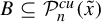 , we have

As we did for the two-dimensional conditional measure
$\tilde {\mu }^{cu}_{n, \tilde {x}}$
 , we also push
$\tilde {\mu }^{u}_{n, \tilde {x}}$
 forward to
${\mathbb R}^2$
 as

a measure supported at
$({\mathbb R} \times \{s\}) \cap \mathcal {Q}^{cu}_n(\tilde {x})$
 , where
$\tilde {y} = \Phi ^c_{\tilde {x}}(s) = \Phi _{\tilde {x}}(0, s)$
 .
Since
$\mathcal {R}_{\tilde {x}}$
 takes conditional measures on
$\widetilde W^{cu}(\tilde {y})$
 to conditional measures with respect to the corresponding partition on
${\mathbb R}^2$
 , we have that

where
$d\nu ^{c}_{n, \tilde {x}}(s) \stackrel {\scriptscriptstyle \textrm {def.}}{=} d(\mathcal {R}_{\tilde {x}})_*\tilde {\mu }^{c}_{n, \tilde {x}}(0,s)$
 and
$B \subset \mathcal {Q}^{cu}_n(\tilde {x})$
 is a Borelian.
As in [Reference Alvarez, Leguil, Obata and SantiagoALOS24, Lemma 7.6], we have the following lemma.
Lemma 3.5. For
$\tilde {\mu }$
 -a.e.
$\tilde {x} \in {\mathbb {T}_f^2}$
 ,
$n \in {\mathbb N}$
 , and
$\nu ^{cu}_{n, \tilde {x}}$
 -a.e.
$(t,s) \in \mathcal {Q}^{cu}_n({\tilde {x}})$
 , we have that

where the density
$\gamma ^u_n(s)$
 does not depend on t.
Consider
$I_1 = [-1, 1] \subseteq {\mathbb R}$
 and
$I = [a,b]$
 with
$a < 0 < b$
 . For
$\tilde {\mu }$
 -a.e.
$\tilde {x} \in {\mathbb {T}_f^2}$
 and
${B \subseteq {\mathbb R}}$
 a Borel subset, there is
$n_0 = n_0(x, I, I_1, B) \in {\mathbb N}$
 such that
$n \geq n_0$
 implies
$I \times (B \cup I_1) \subseteq \mathcal {Q}^{cu}_n(\tilde {x})$
 .
Lemma 3.6. For
$\tilde {\mu }$
 -a.e.
$\tilde {x} \in {\mathbb {T}_f^2}$
 and
$B \subseteq {\mathbb R}$
 a Borel bounded subset, there is
$n_0 \in {\mathbb N}$
 such that
$m> n \geq n_0$
 implies

3.3.1 Proof of Lemma 3.1
Lemma 3.6 allows us to define the leaf-wise quotient measures, by considering
$n \in {\mathbb N}$
 sufficiently large,

which gives us indeed a measure on
${\mathbb R}$
 . Notice that
$\hat {\nu }^c_{\tilde {x}}$
 coincides with
$\nu ^c_{n,x}$
 on
$Q^c_{n}(\tilde {x})$
 (up to normalization). Thus, if
$\hat {\nu }^c_{\tilde {x}}$
 is absolutely continuous, so is
$\nu ^c_{n,\tilde {x}}$
 . By Lemma 3.5, this implies that
$\nu ^{cu}_{n,\tilde {x}}$
 is absolutely continuous with respect to the Lebesgue measure of
${\mathbb R}^2$
 . Since
$\Phi _{\tilde {x}}$
 is
$C^1$
 , this proves that
$\tilde {\mu }^{cu}_{n,\tilde {x}}$
 is absolutely continuous with respect to the Lebesgue measure of the Pesin center manifold
$W^{cu}(\tilde {x})$
 . Thus, Lemma 3.1 follows from Lemma 2.27.
3.4 Basic moves of leaf-wise measures
The following lemma describes how leaf-wise quotient measures change when we move the base point in three different ways. These properties play a crucial role in the argument. The proof is a direct consequence of the definition of leaf-wise quotient measures, the properties of the normal forms given in Proposition 3.2 and Theorem 3.4, and Lemma 3.5. It follows exactly as in [Reference Alvarez, Leguil, Obata and SantiagoALOS24], so we omit it here. We say that two locally finite Radon measures on
${\mathbb R}$
 are proportional and we denote it by
$\mu \propto \nu $
 if
$\mu =c\nu $
 for some
$c>0$
 .
Lemma 3.7. For
$\tilde {\mu }$
 -a.e.
$\tilde {x} \in {\mathbb {T}_f^2}$
 , the following holds:
-
(1) $\hat {\nu }^c_{\tilde {f}(\tilde {x})} \propto (\Lambda ^c_{\tilde {x}})_*\hat {\nu }^c_{\tilde {x}}$
, where
$\Lambda ^c_{\tilde {x}}: {\mathbb R} \to {\mathbb R}$
is given by
$\Lambda ^c_{\tilde {x}}(s) = \unicode{x3bb} ^c_{\tilde {x}}s$
; -
(2) if $\tilde {y} \in \widetilde W^c(\tilde {x})$
, then $$ \begin{align*} \hat{\nu}^c_{\tilde{y}} \propto (h^2_{\tilde{x}, \tilde{y}})_*\hat{\nu}^c_{\tilde{x}}; \end{align*} $$
-
(3) if $\tilde {x}^u\in \widetilde {{\mathcal W}}^u(\tilde {x})$
, then $$ \begin{align*} \hat{\nu}^c_{\tilde{x}^u} \propto (h^2_{\tilde{x}, \tilde{x}^u})_*\hat{\nu}^c_{\tilde{x}}. \end{align*} $$


4 Uniform transversality along fibers
From now on, we start the proof of Theorem 1.1. In this section, our setting is slightly more flexible: we consider
$f:{\mathbb {T}^2}\to {\mathbb {T}^2}$
 a partially hyperbolic, strongly transitive endomorphism and
$\mu $
 an ergodic invariant probability measure (not necessarily a u-Gibbs measure). We consider
$\tilde {f}:{\mathbb {T}_f^2}\to {\mathbb {T}_f^2}$
 and
$\tilde {\mu }$
 the lifts of f and
$\mu $
 to the inverse limit space. Let
$\{\tilde {\mu }_x\}_{x\in {\mathbb {T}^2}}$
 denote the conditional measures of
$\tilde {\mu }$
 with respect to the fibers of
${\mathbb {T}_f^2}$
 .
4.1 The angle function
We can measure angles between vectors in
$T_{\tilde {x}}{\mathbb {T}_f^2}$
 and
$T_{\tilde {y}}{\mathbb {T}_f^2}$
 using the canonical projection
$\pi :{\mathbb {T}_f^2}\to {\mathbb {T}^2}$
 . In particular, this allows us to measure angles between different unstable directions along the fiber
$\Sigma (\tilde {x})$
 .
For
$\tilde {x}\in {\mathbb {T}_f^2}$
 and any given
$\tilde {y}\in \Sigma (\tilde {x})$
 , we denote

Notice that the angle function is continuous in the following sense: if
$\tilde {x}_n\to \tilde {x}$
 and
$\tilde {y}_n\to \tilde {y}$
 , with
$\tilde {y}_n\in \Sigma (\tilde {x}_n)$
 for every
$n\in {\mathbb N}$
 , then
$\lim \alpha (\tilde {x}_n,\tilde {y}_n)=\alpha (\tilde {x},\tilde {y})$
 .
We consider the compact set
${\mathcal P}(\tilde {x})=\{\tilde {y}\in \Sigma (\tilde {x});\alpha (\tilde {x},\tilde {y})=0\}$
 and its complement
${\mathcal N}(\tilde {x})=\Sigma (\tilde {x})\setminus {\mathcal P}(\tilde {x})$
 . The invariance of the unstable bundle implies that

for every
$m\in {\mathbb Z}$
 .
Remark 4.1. Notice that f is special if, and only if,
${\mathcal N}(\tilde {x})=\emptyset $
 for every
$\tilde {x}\in {\mathbb {T}_f^2}$
 .
Our assumptions that f is a strongly transitive transformation of
${\mathbb {T}^2}$
 implies the following lemma.
Lemma 4.2. Assume that f is not special. Then, for every fiber
$\Sigma (\tilde {x})$
 , the set
${\mathcal N}(\tilde {x})$
 is not empty.
Proof. Assume that for some
$\tilde {x}\in {\mathbb {T}_f^2}$
 , the set
${\mathcal N}(\tilde {x})$
 is empty. Take any fiber
$\Sigma (\tilde {a})\subset {\mathbb {T}_f^2}$
 and any point
$\tilde {b}\in \Sigma (\tilde {a})$
 . Then, by Corollary 2.7, there exist sequences of points such that
$\tilde {a}_k\to \tilde {a}$
 and
$\tilde {b}_k\to \tilde {b}$
 , with
$\tilde {b}_k\in \Sigma (\tilde {a}_k)$
 , and, for each k, both points
$\tilde {a}_k$
 and
$\tilde {b}_k$
 belong to
$\tilde {f}^{-k}(\Sigma (\tilde {x}))$
 . By our assumption, this implies that

Since the derivative of f is a linear isomorphism, this implies that

By continuity of the assignment
$(\tilde {x},\tilde {y})\mapsto \alpha (\tilde {x},\tilde {y})$
 , we deduce that

This proves that
${\mathcal N}(\tilde {a})=\emptyset $
 , which implies that f must be special and completes the proof.
By pushing a bit further the above argument, we can obtain an even stronger conclusion.
Lemma 4.3. Assume that f is not special. Then, the set
${\mathcal N}(\tilde {x})$
 is open and dense in the fiber
$\Sigma (\tilde {x})$
 for every
$\tilde {x}\in \Sigma (\tilde {x}).$

Proof. Openness is direct from the definition and the continuity of the function
$(\tilde {x},\tilde {y})\mapsto \alpha (\tilde {x},\tilde {y})$
 . Assume the lemma is false. Then, for some
$\tilde {x}\in {\mathbb {T}_f^2}$
 , the set
${\mathcal P}(\tilde {x})$
 has non-empty interior. In particular, there exists a small cylinder
$I\subset {\mathcal P}(\tilde {x})$
 . By backward expansion along fibers, there must exist an integer
$n>0$
 such that

By (4.1), we deduce that
${\mathcal P}(\tilde {f}^{-n}(\tilde {x}))=\Sigma (\tilde {f}^{-n}(\tilde {x}))$
 , which contradicts Lemma 4.2.
The above result implies the dichotomies presented in [Reference Costa and MicenaCM22, Reference Micena and TahzibiMT16], but for the strongly transitive case.
4.2 The non-transversality set
When f is not special, the strongly transitive assumption implies that in every fiber, there are infinitely many different unstable directions. In our case, this is made explicit by Lemma 4.3. We are now going to consider how the measure
$\tilde {\mu }$
 ‘sees’ these different unstable directions. The natural strategy then is to consider the ‘bad’ set of points for which the measure does not ‘see’ any transversality at all.
Definition 4.1. The non-transversality set is the set
$\tilde {\mathbf {B}}=\{\tilde {x}\in {\mathbb {T}_f^2} : \tilde {\mu }_x({\mathcal N}(\tilde {x}))=0\}$
 .
We have that
$\tilde {\mathbf {B}}$
 is
$\tilde {f}$
 -invariant. Therefore, by ergodicity,
$\tilde {\mu }(\tilde {\mathbf {B}})\in \{0,1\}$
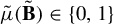 . Notice that
$\tilde {\mathbf {B}}$
 depends on the measure, although, for simplicity, our notation does not reflect that.
Lemma 4.4. Assume that f is not special and that
$\tilde {\mu }(\tilde {\mathbf {B}})=1$
 . Then,
$\operatorname {supp}(\tilde {\mu })$
 has empty interior.
Proof. By Lemma 4.3, it suffices to show that for every
$\tilde {x}\in {\mathbb {T}_f^2}$
 , no point
$\tilde {y}\in {\mathcal N}(\tilde {x})$
 lies in
$\operatorname {supp}(\tilde {\mu })$
 . Take
$\tilde {y}\in {\mathcal N}(\tilde {x})$
 . By continuity, there exists a neighborhood U of
$x=\pi (\tilde {x})$
 such that for every
$\tilde {z}\in \pi ^{-1}(U)\cap \tilde {{\mathcal W}}^{cu}(\tilde {x})$
 , there exists a cylinder
$I(\tilde {z})\subset {\mathcal N}(\tilde {z})$
 . In particular,
$\bigcup _{\tilde {z}\in \pi ^{-1}(U)\cap \tilde {{\mathcal W}}^{cu}(\tilde {x})}I(\tilde {z})$
 is a neighborhood of
$\tilde {y}$
 . Since we assumed
$\tilde {\mu }(\tilde {\mathbf {B}})=1$
 , we have that for almost every
$\tilde {z}$
 , it holds that
$\tilde {\mu }_{\tilde {z}}(I(\tilde {z}))=0$
 . By Rokhlin’s theorem, we deduce that

which implies that
$\tilde {y}\notin \operatorname {supp}(\tilde {\mu })$
 .
4.3 A 0 or 1 law
Let us assume now that
$\mu \in {\mathcal M}^{\operatorname {erg}}_f({\mathbb {T}^2})$
 is a fully supported ergodic invariant measure. We deduce from Lemma 4.4 that for
$\mu $
 -a.e.
$x\in {\mathbb {T}^2}$
 , it holds that
$\tilde {\mu }_x({\mathcal N}(\tilde {x}))>0$
 . That is, under the full support assumption, the measure ‘sees’ some transversality at each fiber. However, in our setting, this is a 0 or 1 law: once some transversality is seen at almost every fiber, we immediately have that the measure actually sees transversality almost everywhere in almost every fiber. More precisely, the goal of this section is to prove the following.
Lemma 4.5. For
$\mu $
 -a.e.
$x\in {\mathbb {T}^2}$
 , it holds that
$\tilde {\mu }_x({\mathcal N}(\tilde {x}))=1$
 .
In our case, we can take advantage of the fractal structure of the fibers and give a point-density proof of the 0 or 1 law that is much simpler then the proof in [Reference Alvarez, Leguil, Obata and SantiagoALOS24], which is based on a martingale convergence argument.
Lemma 4.6. [Reference MillerMil08, Proposition 2.10]
Suppose that
$(X,d)$
 is a compact ultrametric space,
$\mu $
 is a probability measure on X, and B is a Borel set. Then,

for
$\mu $
 -a.e.
$x\in B$
 .
Recall that, by Remark 2.1, each fiber
$\Sigma (\tilde {x})$
 is a compact ultrametric space. In particular, the above lemma applies to the measure
$\tilde {\mu }_x$
 .
4.3.1 Proof of Lemma 4.5
Assume by contradiction the existence of a
$\tilde {\mu }$
 positive measure set
$\tilde {A}$
 such that
$\tilde {\mu }_x({\mathcal P}(\tilde {x}))>0$
 for every
$\tilde {x}\in \tilde {A}$
 . Consider the measurable function

which is positive almost everywhere since
$\tilde {\mu }(B)=0$
 . By Lusin’s theorem, for every
$\delta>0$
 , there exists
$c>0$
 such that
$\tilde {\mu }_x({\mathcal N}(\tilde {x}))\geq c$
 if
$\tilde {x}\in \tilde {K}$
 for some compact set
$\tilde {K}$
 with
$\tilde {\mu }_x(\tilde {K})>1-\delta $
 . Take
$\delta $
 small enough such that
$\tilde {\mu }(\tilde {K}\cap \tilde {A})>0$
 and take
$\tilde {x}\in \tilde {K}\cap \tilde {A}.$
 By Rokhlin’s theorem and ergodicity, we can assume the existence of a point
$\tilde {y}\in {\mathcal P}(\tilde {x})$
 so that
$\tilde {f}^{-n}(\tilde {y})\in \tilde {K}$
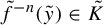 for infinitely many values of n. By Lemma 4.6, we can further assume that
$\tilde {y}$
 is a density point of
${\mathcal P}(\tilde {x})$
 with respect to
$\tilde {\mu }_x$
 .
Observe that, in the metric given in Lemma 4.6, balls are cylinders. Therefore, there exists some cylinder
$\tilde {y}\in I(\tilde {y})\subset \Sigma (\tilde {x})$
 such that

By (4.1), we can take n large enough such that the following properties hold:
-
• $\tilde {f}^{-n}(I(\tilde {y}))\supseteq \Sigma (\tilde {y}_{-n})$
; -
• ${\mathcal P}(\tilde {f}^{-n}(\tilde {y}))=\tilde {f}^{-n}({\mathcal P}(\tilde {y}) \cap I(\tilde {y}))\cap \Sigma (\tilde {y}_{-n})$
; -
• $\tilde {y}_{-n}\stackrel {\scriptscriptstyle \textrm {def.}}{=}\tilde {f}^{-n}(\tilde {y})\in \tilde {K}$
.


The first two properties above imply that

which, in turn, implies that
$\tilde {\mu }_{\tilde {f}^{-n}(\tilde {y})}({\mathcal N}(\tilde {f}^{-n}(\tilde {y})))<c$
 . By the definition of
$\tilde {K}$
 , this contradicts the third property above and completes the proof.
4.4 An Egorov-type estimate of transversality
We can now state our uniform transversality estimate along fibers. The proof is the same as the argument of [Reference Alvarez, Leguil, Obata and SantiagoALOS24, Lemma 11.2], so we refrain from repeating the details.
Proposition 4.7. Given a constant
$\gamma>0$
 and
$K\subset {\mathbb {T}^2}$
 a compact set with
${\mu (K)>1-\gamma} $
 , there exist a constant
$\beta =\beta (\gamma )$
 and a measurable set
$K'\subset K$
 , with
$\tilde {\mu }(K')>1-2\sqrt {\gamma }$
 , such that for every
$\tilde {x}\in K'$
 , there exists a point
$\tilde {y}$
 inside the fiber
$\Sigma (\tilde {x})$
 so that
$\alpha (\tilde {x},\tilde {y})>\beta $
 .
The above lemma is used in §6 in the proof of Lemma 6.4, where we prove that we have ‘abundance’ of the configurations we need to run our argument.
5 Y-configurations: coupling and synchronization
5.1 Stopping times
Remember that the notation
$\hat {\unicode{x3bb} }^c_{\tilde {x}}(n)$
 stands for the Lyapunov norm of the nth derivative restricted to the direction
$E^c$
 , that is,

Consider
$\tilde {x} \in {\mathbb {T}_f^2}$
 and
$\tilde {x}^u \in \widetilde {{\mathcal W}}^u(\tilde {x})$
 . Given a small number
$\varepsilon>0$
 , we define the first stopping time as the function
$\tau :{\mathbb Z}\to {\mathbb Z}$
 defined by

Given the value of
$\tau (n)=\tau (\tilde {x},\tilde {x}^u,n,\varepsilon )$
 , we define

The function
$t:{\mathbb Z}\to {\mathbb Z}$
 is called the second stopping time. We refer to the pair
$(,\tau ,t)$
 as the stopping times. These functions can be computed for
$\tilde {\mu }$
 -a.e.
$\tilde {x}$
 and for all
$\tilde {x}^u \in \widetilde {{\mathcal W}}^u(\tilde {x})$
 by Lemma 2.33.
Remark 5.1. It follows from Remark 2.35 that
$\tau =\tau (\tilde {x},\tilde {x}^u,n,\varepsilon )$
 and
$t=t(\tilde {x},\tilde {x}^u,\ell ,\varepsilon )$
 , so it holds that

and also

for a constant
$C=C(f,\mu )$
 depending only on the map f and the measure
$\mu $
 .
These functions satisfy the following quasi-isometric estimate.
Lemma 5.2. There are constants
$A>0$
 ,
$\Theta> 1$
 (depending only on
$(f,\mu )$
 ) such that for
$\tilde {\mu }$
 -a.e.
$\tilde {x} \in {\mathbb {T}_f^2}$
 and for all
$\tilde {x}^u \in \widetilde {{\mathcal W}}^u(\tilde {x})$
 , and
$m,n \in {\mathbb N}$
 , we have:
-
• $\Theta ^{-1}|m - n|-A\leq |\tau (m)-\tau (n)|\leq \Theta |m - n|+A$
; -
• $\Theta ^{-1}|m - n|-A\leq |t(m)-t(n)|\leq \Theta |m - n|+A$
.


Proof. For a
$\tilde {\mu }$
 -regular point
$\tilde {x} \in {\mathbb {T}_f^2}$
 ,
$\tilde {x}^u \in \widetilde {{\mathcal W}}^u(\tilde {x})$
 , and
$\varepsilon> 0$
 , consider
$\tau (n) = \tau (\tilde {x}, \tilde {x}^u, n, \varepsilon )$
 and
$t(n) = t(\tilde {x}, \tilde {x}^u, n, \varepsilon )$
 . From (5.1), we have

Using (2.2) and Lemma 2.32, the above inequalities imply that

for all
$n \in \mathbb {N}$
 .
By compactness and Lemma 2.8, one easily deduces that there are
$\chi _1^d < \chi _2^d < 0$
 such that

By (5.3), we have, given
$m \in \mathbb {N}$
 ,
$m \geq n$
 , that

Thus,

is given by using Lemma 2.32 and the fact that

The left-hand inequality on (5.3) and the right-hand side of (5.4) imply that

and, by using the remaining inequalities on said equations, we have also

We may assume without loss of generality that
$\varepsilon $
 is small enough so that
$e^{\sigma }\varepsilon <1$
 . Then, by taking the logarithm on the last two inequalities, we have

which gives us the bound for
$\tau $
 .
A similar argument gives us the bound for t. Indeed, the definition of
$t(n)$
 implies that

for all
$n \in \mathbb {N}$
 .
Lemma 2.32 gives us that

which in turn implies

The inequalities from both the above equation and (5.5) imply that

and then, by taking the logarithm, we have

which, using the bound for
$\tau $
 , gives us the bound for t.
Lemma 5.2 is a key point where our argument deviates from [Reference Alvarez, Leguil, Obata and SantiagoALOS24]. Here, we need to work with Lyapunov norms, so that the quasi-isometric estimates for stopping times do not depend on a Lusin set. This is a crucial ingredient that we use in the Fubini-like argument of Eskin and Lindenstrauss (Lemma 6.2).
The five points in the Y configuration and the dynamical relation between them (colour online).

5.2 Y-configurations
We now introduce a dynamical configuration that will be a central tool in our argument.
Definition 5.1. (Y-configurations)
Given points
$\tilde {x}\in {\mathbb {T}_f^2}$
 ,
$\tilde {x}^u\in \widetilde {{\mathcal W}}^u_1(\tilde {x})$
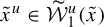 , and numerical parameters
$\ell \in {\mathbb N}$
 ,
$\varepsilon>0$
 , and
$T>1$
 , a
$(\ell ,T) Y$
 -configuration is the data of five points
$(\tilde {x}_{-\ell },\tilde {x},\tilde {x}^u,\tilde {x}^u_m,\tilde {x}_{\hat {m}})$
 (see Figure 2), with the condition that the integers
$m,\hat {m}$
 satisfy

The integers
$m,\hat {m}$
 are to be thought as the two upper (time) lengths of the configuration, while
$\ell $
 is the lower (time) length. Ideally, one would like to have
$m=\tau (\tilde {x},\tilde {x}^u,\ell ,\varepsilon )$
 and
$\hat {m}=t(\tilde {x},\tilde {x}^u,\ell ,\varepsilon )$
 . However, to fully accomplish Eskin and Mirzakhani’s strategy in our context, we need the matching argument, because given two configurations, the stopping times need not be equal. To overcome this difficulty, we use the synchronization idea of Eskin and Lindenstrauss: up to a time length bounded by
$T>0$
 , we can find
$m,\hat {m}$
 such that both configurations are in good matching (see Lemma 6.4).
To emphasize the most relevant data in the definition, we denote a Y-configuration by
$Y(\tilde {x},\tilde {x}^u,\ell ,\varepsilon )$
 .
Definition 5.2. (Quadrilaterals)
Given
$\beta>1$
 and
$\ell \in {\mathbb N}$
 , we say that four points
$\tilde {x},\tilde {x}^u,\tilde {y},\tilde {y}^u$
 generate a
$(\beta ,\ell )$
 -quadrilateral if
$\tilde {x}_{-\ell }\in \Sigma (\tilde {y}_{-\ell })$
 ,
$\tilde {x}^u\in \widetilde {{\mathcal W}}^u(\tilde {x})$
 , and, moreover:
-
(1) $\alpha (\tilde {x}_{-\ell },\tilde {y}_{-\ell })>\beta ^{-1}$
; -
(2) $\beta ^{-1}<d^u(\tilde {x},\tilde {x}^u)<1$
; -
(3) $\tilde {y}^u=H^{cs}_{\tilde {x},\tilde {y}}(\tilde {x}^u)$
.


5.2.1 Center deviation along coupled configurations
When the points
$\tilde {x},\tilde {x}^u,\tilde {y},\tilde {y}^u$
 generate a quadrilateral, we say that the associated configurations
$Y(\tilde {x},\tilde {x}^u,\ell ,\varepsilon )$
 and
$Y(\tilde {y},\tilde {y}^u,\ell ,\varepsilon )$
 are coupled. This notion is devised so that one has a very precise control (up to uniform constants) on the displacement along central leaves after iteration by the stopping times.
The result below follows a similar strategy as [Reference Alvarez, Leguil, Obata and SantiagoALOS24, Lemma 9.2], but we need to be much more careful in our argument due to the lack of uniform expansion on the center. Notice that we also need to require more assumptions regarding which points belong to
${\mathcal L}$
 . In particular, a subtle point is that we discuss a property of configurations whose upper time lengths m,
$\hat {m}$
 are the first and second stopping times, respectively.
Lemma 5.3. Given
${\mathcal L}\subset {\mathbb {T}_f^2}$
 a compact Lusin set,
$\beta>1$
 (see Figures 3 and 4), there exist
$\hat {\beta }=\hat {\beta }(\beta ,{\mathcal L})>1$
 and
$\ell _0=\ell _0({\mathcal L},\beta ,f)$
 such that, if
$\ell \geq \ell _0({\mathcal L})$
 and
$\varepsilon>0$
 are such that there exists some length
$\ell Y$
 -configuration
$Y(\tilde {x},\tilde {x}^u,\ell ,\varepsilon )$
 which is coupled with another Y-configuration
$Y(\tilde {y},\tilde {y}^u,\ell ,\varepsilon )$
 so that
$\tilde {x},\tilde {x}^u,\tilde {y},\tilde {y}^u$
 generate a
$(\beta ,\ell )$
 quadrilateral and such that
$\tilde {x}^u,\tilde {x}^u_\tau \in {\mathcal L}$
 , where
$\tau =\tau (\tilde {x},\tilde {x}^u,\ell ,\varepsilon )$
 is the first stopping time, then

Coupled configurations on
${\mathbb {T}^2}$
 (colour online).

Coupled configurations on the inverse limit space
${\mathbb {T}_f^2}$
 (colour online).

Proof. From the definition of a quadrilateral, we know that
$d^u(\tilde {x},\tilde {x}^u)<1$
 . By the distortion estimate (Lemma 2.38), if we denote by J the segment contained in
$\widetilde {{\mathcal W}}^u(\tilde {x})$
 with end points
$\tilde {x}$
 and
$\tilde {x}^u$
 , we have, for every
$\tilde {z}\in J$
 , that

for every
$j=1,\ldots ,\ell $
 , where
$C=C(f)>1$
 is a constant depending only on f. One deduces that
$d^u(\tilde {x}_{-\ell },\tilde {x}^u_{-\ell })\asymp _C(\unicode{x3bb} ^u_{\tilde {x}_{-\ell }}(\ell ))^{-1}$
 . Thus, the unstable segment
$f^{-\ell }(J)$
 has length
$\asymp _C(\unicode{x3bb} ^u_{\tilde {x}_{-\ell }}(\ell ))^{-1}$
 . Since
$\alpha (\tilde {x}_{-\ell },\tilde {y}_{-\ell })>\beta ^{-1}$
 , a simple geometrical argument, using the continuity of the unstable bundle
$E^u$
 on the space
${\mathbb {T}_f^2}$
 yields
$d^c(\tilde {x}^u_{-\ell },\tilde {y}^u_{-\ell })\asymp _C(\unicode{x3bb} ^u_{\tilde {x}_{-\ell }}(\ell ))^{-1}$
 for every
$\ell \geq \ell _0(\beta )$
 , where the new constant
$C=C(f,\beta )$
 now depends on
$\beta $
 .
We claim that

for some constant
$C=C({\mathcal L},f,\beta )$
 . To prove this claim, first notice that the segment of center manifold joining the points
$\tilde {x}^u$
 and
$\tilde {y}^u$
 is contained inside the local Pesin manifold
$\widetilde W^c_{{\operatorname {loc}}}(\tilde {x}^u)$
 . Indeed, from the distortion Lemma 2.28, we deduce that

for some constant
$C=C({\mathcal L},\tilde {f},\beta )$
 , depending also on
${\mathcal L}$
 . Since
$d^c(\tilde {x}^u_{-\ell },\tilde {y}^u_{-\ell })\asymp _C(\unicode{x3bb} ^u_{\tilde {x}_{-\ell }}(\ell ))^{-1}$
 , the domination of the partial hyperbolic splitting implies that
$d^c(\tilde {x}^u_{-\ell },\tilde {y}^u_{-\ell })$
 is exponentially smaller than the length of
$\tilde {f}^{-\ell }(\widetilde W^c_{{\operatorname {loc}}}(\tilde {x}^u))$
 . Therefore, for
$\ell $
 sufficiently large (depending on the constant
$C({\mathcal L},\beta ,f))$
 , we have that the entire center segment with endpoints
$\tilde {x}^u$
 and
$\tilde {y}^u$
 is contained in the local Pesin manifold
$\widetilde W^c_{{\operatorname {loc}}}(\tilde {x}^u)$
 . The distortion Lemma 2.28 then yields

Now, the claim follows, for on the Lusin set
${\mathcal L}$
 , the quantity
${\mathcal R}^c_{\tilde {x}^u}(\tilde {y}^u)$
 is uniformly comparable to
$d^c(\tilde {x}^u,\tilde {y}^u)$
 .
Since the dynamics acts as a linear expansion on normal forms, this gives us that

Since
$\tilde {x}^u_\tau \in {\mathcal L}$
 , we have that
$\unicode{x3bb} ^c_{\tilde {x}^u}(\tau )$
 and
$\hat {\unicode{x3bb} }^c_{\tilde {x}^u}(\tau )$
 are comparable by a constant depending on
${\mathcal L}$
 . The lemma now follows from Remark 5.1.
Our argument above also yields the following distortion estimate.
Lemma 5.4. Under the same assumptions as in Lemma 5.3, there exists a constant
${C=C({\mathcal L},\beta ,f)>1}$
 such that, for every
$\varepsilon>0$
 sufficiently small:
-
(1) $({\hat {\unicode{x3bb} }^c_{\tilde {x}^u}(\tau )}/{\hat {\unicode{x3bb} }^c_{\tilde {y}^u}(\tau )})\asymp _C 1$
and -
(2) $({\unicode{x3bb} ^c_{\tilde {x}^u}(\tau (\ell ))}/{\unicode{x3bb} ^c_{\tilde {y}^u}(\tau (\ell ))})\asymp _C 1$
.


Proof. The first estimate follows since
$\hat {\beta }\varepsilon <\inf \{r(\tilde {x});\tilde {x}\in {\mathcal L}\}$
 if
$\varepsilon $
 is small enough, and one can apply Lemma 2.36. For the second estimate, we can change from the Lyapunov norm at time m to the background norm, since they are comparable by a constant which depends on
${\mathcal L}$
 and the conclusion follows.
In the next subsection, we are going to prove a fundamental property about coupled configurations: their stopping times cannot differ too much.
5.3 Synchronization of stopping times
The following result plays a substantial role in our application of the factorization method for it allows us to use the same stopping time for both Y-configurations once they are coupled. Before stating the result, we need a definition.
Definition 5.3. Given
$Y(\tilde {x},\tilde {x}^u,\varepsilon ,\ell )$
 a Y-configuration, the unstable dynamical ball associated with the configuration is the set

where
$\tau =\tau (\tilde {x},\tilde {x}^u,\varepsilon ,\ell )$
 is the stopping time.
Proposition 5.5. (Synchronization)
Given
${\mathcal L}\subset {\mathbb {T}_f^2}$
 a compact Lusin set and
$\beta>1$
 , there exists
$T=T({\mathcal L},\beta ,f,\mu )>1$
 such that if
$(\tilde {x},\tilde {x}^u,\tilde {y},\tilde {y}^u)$
 is a
$(\beta ,\ell )$
 -quadrilateral such that
$\tilde {x},\tilde {x}^u,\tilde {x}^u_{\tau (\ell )},\tilde {y}\in {\mathcal L}$
 , where
$\tau (\ell )=\tau (\tilde {x},\tilde {x}^u,\ell ,\varepsilon )$
 , then for every
$\tilde {a}\in J(\tilde {x}^u)$
 and every
$\tilde {b}\in J(\tilde {y}^u)$
 , we have that

Although the proof has some technicalities, the idea is rather simple: on one hand, by Lemma 5.4, we have a bounded distortion estimate for the center derivative at the first stopping time
$\tau (\tilde {x},\tilde {x}^u,\ell ,\varepsilon )$
 ; on the other hand, the exponentially small quantities
$d^{\ell }_{\tilde {x}}$
 and
$d^{\ell }_{\tilde {y}}$
 are comparable since they come from a Hölder cocycle, and
$\tilde {x}$
 and
$\tilde {y}$
 lie on the same fiber (hence become exponentially close in the future), by Lemma 2.28. Since the first stopping time is the time required to increase from
$d^{\ell }_{\tilde {x}}$
 to
$\varepsilon $
 and since the second stopping time is the time required to increase from
$\hat {\unicode{x3bb} }^c_{\tilde {x}}$
 to
$\hat {\unicode{x3bb} }^c_{\tilde {x}}(\tau )$
 , Proposition 5.5 must hold.
5.3.1 Proof of Proposition 5.5
We begin by comparing the stopping times at
$\tilde {x}^u$
 and
$\tilde {y}^u$
 . This is the key point in our implementation of the factorization method: we need only to assume good properties (continuity inside the Lusin set) for the Y-configuration on
$\tilde {x}$
 . In our case, the idea is that we are able to ‘transfer’ some of these properties to the Y-configuration on
$\tilde {y}$
 .
Lemma 5.6. Given
${\mathcal L}\subset {\mathbb {T}_f^2}$
 a compact Lusin set and
$\beta>1$
 , there exists
${T_0=T_0({\mathcal L},\beta ,f,\mu )>1}$
 such that, if
$(\tilde {x},\tilde {x}^u,\tilde {y},\tilde {y}^u)$
 is a
$(\beta ,\ell )$
 -quadrilateral satisfying that
$\tilde {x},\tilde {x}^u,\tilde {x}^u_{\tau (\ell )}\in {\mathcal L}$
 , where
$\tau (\ell )=\tau (\tilde {x},\tilde {x}^u,\ell ,\varepsilon )$
 , then we have that

Proof. Let us denote
$\tau =\tau (\tilde {x},\tilde {x}^u,\varepsilon ,\ell )$
 and
$\hat {\tau }=\tau (\tilde {y},\tilde {y}^u,\varepsilon ,\ell )$
 . Assume first that
$\tau>\hat {\tau }$
 . Then, from the definition, we get

However, we can write

for some constant
$C=C({\mathcal L},\beta ,f)$
 . Indeed, for the first factor on the right-hand side of the equality, we can apply the distortion lemma for the Hölder cocycle
$\tilde {a}\mapsto d^{\ell }_{\tilde {a}}$
 and points on the same fiber, and lower bound it by a constant depending only on f. The second factor is bounded by a constant depending on
${\mathcal L}$
 and
$\beta $
 due to Lemma 5.4. The third factor is lower bounded by the exponential due to Lemma 2.32.
Combining these two estimates, we deduce that, whenever k is large enough so that
$Ce^{k\unicode{x3bb} }\geq 1$
 , we are forced to have
${d^\ell _{\tilde {x}}\hat {\unicode{x3bb} }^c_{\tilde {x}^u}(\hat {\tau }+k)}\geq \varepsilon $
 , which proves that
$\tau $
 cannot be larger than
$\hat {\tau }+k$
 .
Observe that, in the above argument, the roles of
$\tilde {x}$
 ,
$\tilde {y}$
 and
$\tilde {x}^u$
 ,
$\tilde {y}^u$
 are reversible. In fact, as we assumed that
$\tilde {y}\in {\mathcal L}$
 , we have that
$\tilde {y}$
 is, in particular, a
$\mu $
 -generic point and so is every
$\tilde {y}^u\in \widetilde {{\mathcal W}}^u(\tilde {y})$
 . Thus, Lemma 2.32 applies to
$\tilde {y}^u$
 as well. As a consequence, we can perform the same argument if we assume
$\hat {\tau }>\tau $
 and, thus,
$|\tau -\hat {\tau }|$
 is bounded by a constant depending on
${\mathcal L},\beta ,f$
 .
We now treat the function t. We define t and
$\hat {t}$
 in a similar fashion. Assume
$t>\hat {t}$
 . We have, from the definition, that

However, we can bound

for some constant
$C=C({\mathcal L},\beta ,f)$
 . Indeed, the first two factors are bounded by the distortion estimates for the Lyapunov norm, while for the third factor, we consider the lower bound in Lemma 2.31 and the fact that
$|\hat {\tau }-\tau |$
 is bounded by a constant depending on
${\mathcal L},\beta ,f$
 . The case
$\hat {t}>t$
 is treated in the same way as before.
We now consider the oscillations of the first stopping time function inside dynamical balls. More precisely, we have the following lemma.
Lemma 5.7. There exists a constant
$C=C(f,\mu )$
 depending only on the map f and the measure
$\mu $
 such that for
$\tilde {\mu }$
 -a.e.
$\tilde {x}\in {\mathbb {T}_f^2}$
 , for every
$\tilde {x}^u\in \widetilde {{\mathcal W}}^u_2(\tilde {x})$
 , given
$\tilde {a}\in J(\tilde {x}^u)$
 , it holds that

Proof. We first describe the choice of the constant
$C=C(f,\mu )$
 . Consider the constant
$0<\unicode{x3bb} <L^c(\mu )$
 , used in Lemma 2.32 and in Remark 2.35. Given this choice (which is already fixed), we consider
$C_1(f,\mu )$
 the constant given in Remark 2.35. Now, let
${C_2=C_2(f,\mu )}$
 be large enough so that if
$k>C_2(f,\mu )$
 , then

We shall prove that the lemma holds with
$C=C_2$
 . Indeed, let us denote
$\tau \stackrel {\scriptscriptstyle \textrm {def.}}{=}\tau (\tilde {x},\tilde {x}^u,\varepsilon ,\ell )$
 and
$\tau _a\stackrel {\scriptscriptstyle \textrm {def.}}{=}\tau (\tilde {x},\tilde {a},\varepsilon ,\ell )$
 .
Assume that
$\tau _a>\tau $
 . Then, by Remarks 2.35 and 5.1, if
$k>C_2(f\mu )$
 , then

This proves that
$\tau _a-\tau \leq C_2(f,\mu )$
 . If
$\tau>\tau _a$
 , one reverses the roles of
$\tilde {x}^u$
 and
$\tilde {a}$
 in the above argument to conclude that
$\tau -\tau _a\leq C_2(f,\mu )$
 . This establishes our claim and completes the proof.
Proof of Proposition 5.5
First, notice that it suffices to give the proof for the first stopping time for the estimate on the second stopping times follows using Remark 5.1. Now, we apply Lemmas 5.7 and 5.6 obtaining

which concludes the proof.
5.4 The geometry of unstable dynamical balls
We now combine several applications of the fundamental distortion Lemma 2.28.
Lemma 5.8. Given
${\mathcal L}\subset {\mathbb {T}_f^2}$
 a compact Lusin set and
$\beta>1$
 , there exists a constant
$L=L({\mathcal L},\beta ,T)>1$
 such that for every
$\varepsilon>0$
 small enough, whenever
$\ell \in {\mathbb N}$
 is large enough and
$\varepsilon $
 is small enough, if
$(\tilde {x},\tilde {x}^u,\tilde {y},\tilde {y}^u)$
 is a
$(\beta ,\ell )$
 quadrilateral such that
$\tilde {x},\tilde {x}^u,\tilde {x}^u_{\tau (\ell )}\in {\mathcal L}$
 , we have for every
$a\in J(\tilde {x}^u)$
 and
$b\in J(\tilde {y}^u)$
 that

for every
$0\leq j\leq \max \{\tau (\tilde {x},\tilde {x}^u,\varepsilon ,\ell ),\tau (\tilde {y},\tilde {y}^u,\varepsilon ,\ell )\}$
 and
$* \in \{c,u\}$
 .
Proof. Consider the point
$\tilde {z}^u\in \Sigma (\tilde {x}^u)$
 such that
$\tilde {y}^u$
 and
$\tilde {z}^u$
 belong to the same center manifold on
${\mathbb {T}_f^2}$
 . From Lemma 5.4, it follows that for
$\varepsilon>0$
 small enough (depending on the Lusin set
${\mathcal L}$
 ), we have that
$y^u\in W^c_{{\operatorname {loc}}}(x^u)$
 . Therefore, in the equality

we can bound the second term by a constant
$C({\mathcal L})$
 , due to Lemma 2.28, while the third term is bounded by a constant
$C(f)$
 , also by Lemma 2.28. By definition of the stopping time, by Lemmas 2.29, 2.30, and 5.7, the first and the fourth term are bounded by a constant
$C({\mathcal L})$
 .
Lemma 5.8, together with the distortion estimates given on Lemma 2.29, implies the following result. The proof follows as in [Reference Alvarez, Leguil, Obata and SantiagoALOS24, Corollary 10.6].
Corollary 5.9. Given
${\mathcal L}\subset {\mathbb {T}_f^2}$
 a compact Lusin set and
$\beta>1$
 , there exists a constant
$L=L({\mathcal L},\beta ,T)>1$
 such that whenever
$\ell \in {\mathbb N}$
 is large enough and
$(\tilde {x},\tilde {x}^u,\tilde {y},\tilde {y}^u)$
 is a
$(\beta ,\ell )$
 quadrilateral such that
$\tilde {x},\tilde {x}^u,\tilde {x}^u_{\tau (\ell )}\in {\mathcal L}$
 , we have that

for every
$0\leq j\leq \max \{\tau (\tilde {x},\tilde {x}^u,\varepsilon ,\ell ),\tau (\tilde {y},\tilde {y}^u,\varepsilon ,\ell )\}+T$
 .
6 Y-configurations: the matching argument
In this section, we are going to prove the main technical result needed to establish Theorem 1.1. The goal is to find pairs of coupled Y configurations
$Y(\tilde {x},\tilde {x}^u,\ell ,\varepsilon )$
 and
$Y(\tilde {y},\tilde {y}^u,\ell ,\varepsilon )$
 such that both dynamical balls
$J(\tilde {x}^u)$
 and
$J(\tilde {y}^u)$
 intersect some Lusin set.
The main idea of this section (which comes from [Reference Eskin and MirzakhaniEM18]) is to transfer information from the the first Y-configuration
$Y(\tilde {x},\tilde {x}^u,\varepsilon ,\ell )$
 to the second one,
$Y(\tilde {y},\tilde {y}^u,\varepsilon ,\ell )$
 , so that we have more flexibility to find ‘good points’ in
$J(\tilde {y}^u)$
 .
6.1 The Fubini argument of Eskin and Lindenstrauss
Consider
$\delta>0$
 and
$K\subset {\mathbb {T}_f^2}$
 a compact subset of measure
$\mu (K)>1-\delta $
 . The result below is a simple consequence of Birkhoff’s ergodic theorem and Egorov’s theorem of measure theory. See [Reference Alvarez, Leguil, Obata and SantiagoALOS24, Lemma 11.4] for a proof.
Lemma 6.1. There exists a compact set
$K^\circ \subset K$
 still of measure
$\mu (K^\circ )>1-\delta $
 and an integer
$T=T(\delta )>1$
 such that, whenever
$n\geq T$
 , one has

for every
$\tilde {x}\in K^\circ $
 .
We let
$\xi ^u$
 be a measurable partition of
${\mathbb {T}_f^2}$
 subordinate to the lamination
$\widetilde {{\mathcal W}}^u$
 . Given a pair
$(\tilde {x},\tilde {x}^u)$
 such that
$\tilde {x}^u\in \xi ^u(\tilde {x})$
 , we define the subset of integers

Given
$\tilde {x}\in {\mathbb {T}_f^2}$
 and an integer
$\ell \in {\mathbb N}$
 , let us consider the set

Considering a continuous function
$\eta :[0,1]\to [0,\infty )$
 with
$\eta (0)=0$
 and an integer
$\ell \in {\mathbb N}$
 , we define the set

This is the set of points
$\tilde {x}\in {\mathbb {T}_f^2}$
 for which one has ‘a large set to choose
$\tilde {x}^u\in \xi ^u(\tilde {x})$
 from’ so that the length-
$\ell Y$
 -configuration
$Y(\tilde {x},\tilde {x}^u,\ell ,\varepsilon )$
 has all its four upper points being ‘highly recurrent’ to the compact set K. This high recurrence is used in the end of Lemma 6.4 to obtain simultaneous returns to K.
The following result has the same proof as [Reference Alvarez, Leguil, Obata and SantiagoALOS24, Lemma 11.4], so we refrain from repeating the details.
Lemma 6.2. There exists a continuous function
$\eta :[0,1]\to [0,\infty )$
 , with
$\eta (0)=0$
 , (which depends only on f) so that the set
$D(\delta ,K)\stackrel {\scriptscriptstyle \textrm {def.}}{=}\{\ell \in {\mathbb N};\tilde {\mu }(K(\ell ))>1-\eta (\delta )\}$
 satisfies

for every
$n>T(\delta )$
 .
6.2 The Eskin–Mirzakhnani combinatorial lemma
The (combinatorial) result below is largely inspired by [Reference Eskin and MirzakhaniEM18] and, though elementary, it is one of the key ideas of our matching argument.
Lemma 6.3. Let
$\Delta>1$
 ,
$m\in {\mathbb N}$
 and
$\eta _1,\eta _2\in (0,1)$
 be numerical constants satisfying the following assumptions:
-
• $1-\eta _1>0.5$
; and -
• $\Delta m\eta _2<0.5$
.


Assume that
$(X,\nu ,{\mathcal B})$
 and
$(Y,\hat {\nu },\hat {{\mathcal B}})$
 are probability spaces, each endowed with a finite collection
$\{J_1,\ldots ,J_k\}\subset {\mathcal B} $
 and
$\{\hat {J}_1,\ldots ,\hat {J}_k\}\subset \hat {{\mathcal B}}$
 of measurable sets so that the following three properties are satisfied:
-
(1) $X=J_1 \cup \cdots \cup J_k$
and
$Y=\hat {J}_1\cup \cdots \cup \hat {J}_k$
; -
(2) if $y\in Y$
, then
$\operatorname {card}\{i\in [1,k];y\in \hat {J}_i\}\leq m$
; -
(3) $\nu (J_i)\asymp _{\Delta }\hat {\nu }(\hat {J}_k)$
.


Suppose that there exist measurable sets
$Q \subset X$
 and
$\hat {Q} \subset Y$
 so that

Then, there exists
$i\in [1,k]$
 so that
$J_i\cap Q\neq \emptyset $
 and
$\hat {J}_i\cap \hat {Q}\neq \emptyset $
 .
Proof. Let
$I(X)\stackrel {\scriptscriptstyle \textrm {def.}}{=}\{i\in [1,k]; J_i\cap Q\neq \emptyset \}$
 and
$I(Y)\stackrel {\scriptscriptstyle \textrm {def.}}{=}\{i\in [1,k]; \hat {J}_i\cap \hat {Q}\neq \emptyset \}$
 . Assume that
$I(X)\cap I(Y)=\emptyset $
 . Then,

which is a contradiction.
6.3 Good matching of Y-configurations
We consider, given
$\delta>0$
 , a compact Lusin set
${\mathcal L}\subset {\mathbb {T}_f^2}$
 with
$\tilde {\mu }({\mathcal L})>1-\delta $
 . Given numbers
$\beta>1$
 ,
$T>1$
 , and a compact subset K of measure
$\tilde {\mu }(K)>1-\delta $
 , we say that a pair
$Y(\tilde {x},\tilde {x}^u,\varepsilon ,\ell )$
 and
$Y(\tilde {y},\tilde {y}^u,\varepsilon ,\ell )$
 of
$(\ell ,T)$
 -Y-configurations are in good matching relatively to
$(K,{\mathcal L},T,\beta )$
 if:
-
(1) $(\tilde {x},\tilde {x}^u,\tilde {y},\tilde {y}^u)$
is a
$(\beta ,\ell )$
quadrilateral; -
(2) $\tilde {x},\tilde {y}\in K\cap {\mathcal L}$
; -
(3) there exist $\tilde {a}\in J(\tilde {x}^u)\cap K\cap {\mathcal L}$
,
$\tilde {b}\in J(\tilde {y}^u)\cap K\cap {\mathcal L}$
, and
$m\in (\tau (\ell )-T,\tau (\ell )-T)$
such that
$\tilde {a}_m,\tilde {b}_m\in K\cap {\mathcal L}$
; and -
(4) there exists $\widehat {m}\in (t(\ell )-T,t(\ell )+T)$
such that
$\tilde {x}_{\widehat {m}},\tilde {y}_{\widehat {m}}\in K\cap {\mathcal L}$
.


The main result of this section which is also our main ingredient to prove Theorem 1.1 is the following. For the statement, we recall the following definition: we say that a subset
$D\subset {\mathbb N}$
 of integers has positive density if

In particular, notice that every positive density subset
$D\subset {\mathbb N}$
 is an infinity set.
Lemma 6.4. There exist constants
$\delta>0$
 ,
$\beta>1$
 ,
$T>1$
 , and a Lusin set
${\mathcal L}$
 with measure
$\tilde {\mu }({\mathcal L})>1-\delta $
 such that: for every compact set K with
$\tilde {\mu }(K)>1-2\delta $
 , there exists a subset
$D\subset {\mathbb N}$
 with positive density such that for every
$\ell \in D$
 large enough and every
$\varepsilon>0$
 small enough, one can find a pair
$Y(\tilde {x},\tilde {x}^u,\varepsilon ,\ell )$
 and
$Y(\tilde {y},\tilde {y}^u,\varepsilon ,\ell )$
 of
$(\ell ,T)$
 -Y-configurations which are in good matching relatively to
$(K,{\mathcal L},T,\beta )$
 .
The proof of Lemma 6.4 is rather involved. For the sake of clarity, we shall present it in several steps. This result is parallel to [Reference Alvarez, Leguil, Obata and SantiagoALOS24, Proposition 11.8]. The main difference in our case is that we consider non-uniform expansion along the center direction and thus we need to be much more careful with the choice of constants.
Let us give now a brief sketch of the argument: we choose
${\mathcal L}_1\subset {\mathcal L}_2$
 , two Lusin sets along with constants
$\delta _2<<\delta _1$
 so that
$\tilde {\mu }({\mathcal L}_i)>1-\delta _i$
 ,
$i=1,2$
 . With the set
${\mathcal L}_1$
 , we apply Proposition 4.7 and obtain a constant
$\beta _1>1$
 . With this constant, we apply the synchronization of stopping times (Proposition 5.5) and find a constant
$T_1>1$
 . Once these parameters are fixed, we can produce many coupled
$(\ell ,T_1)-Y-$
 configurations. However, the definition of good matching requires the six points
$\tilde {x},\tilde {y},\tilde {a},\tilde {b},\tilde {a}_m,\tilde {b}_m,\tilde {x}_{\hat {m}}$
 , and
$\tilde {y}_{\hat {m}}$
 to lie inside the Lusin set. So, our strategy is to use the Lusin set
${\mathcal L}_1$
 to give uniform estimations allowing us to search for a configuration in good matching relatively to the larger Lusin set
${\mathcal L}_2$
 .
The rest of this section is devoted to the formal proof of Lemma 6.4.
6.3.1 First step: choice of
$\delta _1$

As we announced before, we choose
${\mathcal L}_1$
 , a Lusin set along with a constant
$\delta _1$
 so that
$\tilde {\mu }({\mathcal L}_1)>1-\delta _1$
 . We shall first choose and fix
$\delta _1$
 .
Consider the function
$\eta :[0,1]\to [0,\infty )$
 given in Lemma 6.2 and let us denote
$\eta _1\stackrel {\scriptscriptstyle \textrm {def.}}{=}\eta (\delta _1)$
 . We consider
$\gamma =\delta _1$
 in Proposition 4.7 and let
$\beta _1=\beta (\delta _1)$
 be the constant given by that proposition. We consider the constants
$T_1\stackrel {\scriptscriptstyle \textrm {def.}}{=} T({\mathcal L}_1,\beta _1)$
 to be the constant given in the synchronization Proposition 5.5. We take
$\delta _1$
 sufficiently small so that
$1-\eta _1>0.6$
 and

With this choice of
$\delta _1$
 , we fix a Lusin set
${\mathcal L}_1$
 with measure
$\tilde {\mu }({\mathcal L}_1)>1-\delta _1$
 .
6.3.2 Second step: choice of
$\delta _2$

We shall now choose
$\delta _2<<\delta _1$
 . For this, we will need a series of lemmas giving numbers depending on the value of
$\delta _1$
 , previously fixed.
Lemma 6.5. (Overlap control of unstable dynamical balls)
There exists a constant
${m=m({\mathcal L}_1)}$
 with the following property. Assume that
$(\tilde {x},\tilde {x}^u,\tilde {y},\tilde {y}^u)$
 is a
$(\beta _1,\ell )$
 -quadrilateral with
$\tilde {x},\tilde {y}\in {\mathcal L}_1$
 . Given a compact set
$Q\subset \widetilde {{\mathcal W}}^u_1(\tilde {x})\cap {\mathcal L}_1$
 with
$\tilde {\mu }(Q)>1-\eta _1$
 , given any finite cover
$X=\bigcup _{i=1}^kJ_i$
 of

by unstable dynamical balls
$J_i=J^u(\tilde {x}^u_i)$
 such that for every
$\tilde {z}\in \widetilde {{\mathcal W}}^u_1(\tilde {x})$
 ,

defining
$\tilde {y}^u_i=H^{cs}_{\tilde {x},\tilde {y}}(\tilde {x}^u_i)$
 and
$\hat {J}_i\stackrel {\scriptscriptstyle \textrm {def.}}{=} J^u(\tilde {y}^u_i)$
 , then for every
$\tilde {b}\in \widetilde {{\mathcal W}}^u_1(\tilde {y})$
 ,

Proof. Take a point
$\tilde {b}\in \widetilde {{\mathcal W}}^u(\tilde {y})$
 and denote by

all the intervals within the collection
$\{\hat {J}_1,\ldots ,\hat {J}_k\}$
 that contains the point
$\tilde {b}$
 . Consider
$J\stackrel {\scriptscriptstyle \textrm {def.}}{=}\bigcup _{j=1}^mJ_{i_j}$
 and
$\hat {J}\stackrel {\scriptscriptstyle \textrm {def.}}{=}\bigcup _{j=1}^m\hat {J}_{i_j}$
 . We shall bound from above the length of
$\hat {J}$
 and from below the length of J. The estimate on m will then follow from the Hölder continuity of center holonomies.
For simplicity, we also denote

Let
$\mathcal {T}\stackrel {\scriptscriptstyle \textrm {def.}}{=}\{\tau _{i_1},\ldots ,\tau _{i_m},\hat {\tau }_{i_1},\ldots ,\hat {\tau }_{i_m}\}$
 and define
$\tau ^*\stackrel {\scriptscriptstyle \textrm {def.}}{=}\min \mathcal {T}$
 . For the bound on
$\hat {J}$
 , one observes that
$\tilde {f}^{\tau ^*}(\tilde {b})\in \tilde {f}^{\tau ^*}(\hat {J}_{i_j})$
 for every
$j=1,\ldots ,m$
 . Since
$|\tilde {f}^{\tau ^*}(\hat {J}_{i_j})|\leq 2$
 , it follows that
$|\hat {J}|\leq 4$
 .
For the bound on J, since no more than two intervals
$J_{i_j}$
 overlap at a time, we can estimate

However, one has, by definition of a dynamical ball, that
$|\tilde {f}^{\tau _{i_j}}(J_{i_j})|=2$
 . Also, by Proposition 5.5, we have that
$|\tau _{i_j}-\tau (\tilde {y},\tilde {b},\varepsilon ,\ell )|<T({\mathcal L}_1,\beta _1)$
 and also
$|\hat {\tau }_{i_j}-\tau (\tilde {y},\tilde {b},\varepsilon ,\ell )|< T({\mathcal L}_1,\beta _1)$
 for every
$j=1,\ldots ,m$
 . Thus, by the triangle inequality, we have that for every
$\tau \in \mathcal {T}$
 , it holds that

These two facts together imply that

where
$\xi (f)=\max \{\|Df(x)v\|/\|v\|;x\in {\mathbb {T}^2},v\in T_x{\mathbb {T}^2}\}$
 and
$T_1=T_1({\mathcal L}_1,\beta _1)$
 is a constant that depends on the Lusin set
${\mathcal L}_1$
 . Thus,

Since J is a segment of unstable manifold, there must exist a pair of points
$\tilde {a},\tilde {a}^{\prime }$
 on J such that
$d^u(\tilde {a},\tilde {a}^{\prime })>me^{-\xi (f)T_1}$
 . Since every point of J is at a distance of at most 1 from some
$\tilde {x}^u_{i_j}$
 , we conclude that there must exist a pair of points
$x^u_{i_j}$
 and
$x^u_{i_r}$
 on
${\mathcal W}^u(\tilde {x}_{\tau ^*})$
 such that

By the Hölder continuity of the center bundle, we have that

We deduce that

with
$T_1=T_1({\mathcal L}_1,\beta _1)$
 . This ends the proof.
Remark 6.6. In our argument, the constant
$m({\mathcal L}_1)$
 appearing in the lemma above depends on our first choice of Lusin set
${\mathcal L}_1$
 , which we use to have uniform estimates allowing us to put all eight points of the main picture in Figure 1 in a larger Lusin set
${\mathcal L}_2$
 , while in [Reference Alvarez, Leguil, Obata and SantiagoALOS24], the constant is uniform (depending only on the dynamical system).
In the same setting as above, we need to determine another constant which compares the lengths of the unstable dynamical balls
$J_i,\hat {J}_i$
 .
Lemma 6.7. There exists a constant
$\Delta =\Delta ({\mathcal L}_1)$
 with the following property. Assume that
$(\tilde {x},\tilde {x}^u,\tilde {y},\tilde {y}^u)$
 is a
$(\beta _1,\ell )$
 -quadrilateral, with
$\tilde {x},\tilde {y}\in {\mathcal L}_1$
 . Given a compact set
${Q\subset \widetilde {{\mathcal W}}^u_1(\tilde {x})\cap {\mathcal L}_1}$
 with
$\tilde {\mu }(Q)>1-\eta _1$
 , given any finite cover
$X=\bigcup _{i=1}^kJ_i$
 of

by unstable dynamical balls
$J_i=J^u(\tilde {x}^u_i)$
 such that for every
$\tilde {z}\in \widetilde {{\mathcal W}}^u_1(\tilde {x})$
 ,

defining
$\tilde {y}^u_i=H^{cs}_{\tilde {x},\tilde {y}}(\tilde {x}^u_i)$
 and
$\hat {J}_i\stackrel {\scriptscriptstyle \textrm {def.}}{=} J^u(\tilde {y}^u_i)$
 , if
$X=\bigcup _{i=1}^kJ_i$
 and
$Y=\bigcup _{i=1}^k\hat {J}_i$
 are the normalized probabilities

satisfy

for every
$i=1,\ldots ,k$
 .
Proof. On one hand, it follows from Corollary 5.9 that
$|J_i|\asymp _C|\hat {J}_i|$
 for some constant
$C=C({\mathcal L}_1,\beta )$
 . From Lemma 2.23, we may enlarge this constant (but still depending only on
${\mathcal L}_1$
 ) so that
$\tilde {\mu }^u_{\tilde {x}}(J_i)\asymp _{C}\tilde {\mu }^u_{\tilde {y}}(\hat {J}_i)$
 . Lemma 6.5 allows us to estimate

and a similar reasoning gives an upper bound which shows that
$|X|$
 and
$|Y|$
 are comparable up to some constant
$\hat {C}=\hat {C}({\mathcal L}_1,\beta )$
 . Using Lemma 2.23, we may enlarge
$\hat {C}$
 (but still depending only on
${\mathcal L}_1$
 ) if necessary to have that
$\tilde {\mu }^u_{\tilde {x}}(X)\asymp _{\hat {C}}\tilde {\mu }^u_{\tilde {y}}(Y)$
 . Putting all these estimates together, one deduces that the probabilities
$\nu =\tilde {\mu }^u_{\tilde {x}}|_X/\tilde {\mu }^u_{\tilde {x}}(X)$
 and
$\hat {\nu }=\tilde {\mu }^u_{\tilde {y}}|_Y/\tilde {\mu }^u_{\tilde {y}}(Y)$
 satisfy

for every
$i=1,\ldots ,k$
 and for some constant
$\Delta =\Delta ({\mathcal L}_1)$
 , as claimed.
Remark 6.8. The argument above also gives, as a by product, that
$\tilde {\mu }^u_{\tilde {y}}(Y)\geq \zeta>0$
 for some uniform constant
$\zeta =\zeta ({\mathcal L}_1)$
 .
We are now in a position to give our choice of the constant
$\delta _2$
 . Let
$\zeta ({\mathcal L}_1)$
 be the constant given in Remark 6.8. Since
$\eta _2=\eta (\delta _2)\to 0$
 as
$\delta _2\to 0$
 , we may choose
$\delta _2$
 small enough so that

Once
$\delta _2$
 is fixed by (6.4), we choose a larger Lusin set
${\mathcal L}_2\supset {\mathcal L}_1$
 with measure
${\tilde {\mu }({\mathcal L}_2)>1-\delta _2}$
 .
6.3.3 Third step: final choice of constants and sets
We take
$\delta =\delta _2/10$
 and
${\mathcal L}\supset {\mathcal L}_2$
 a Lusin set with
$\tilde {\mu }({\mathcal L})>1-\delta $
 . Let
$\beta =\beta _1$
 . To complete the constants and sets announced in Lemma 6.4, it only remains to define
$T>1$
 . Let
$T=T(\delta _1)$
 be chosen large enough, so that, given any compact set K with measure
$\tilde {\mu }(K)>1-\delta _1$
 , the set of points
$\tilde {x}\in {\mathbb {T}_f^2}$
 for which (6.1) holds has measure larger than
$1-\delta _1$
 . Notice that the existence of T depending only on
$\delta _1$
 is ensured by Lemma 6.1. Enlarging this choice, if necessary, we may further assume that
$T\geq T({\mathcal L}_1,\beta _1)$
 , where
$T({\mathcal L}_1,\beta _1)$
 is the constant given by the synchronization Proposition 5.5.
We claim that Lemma 6.4 holds with these choices.
6.3.4 Fourth step: finding the configurations
Let
$K\subset {\mathbb {T}_f^2}$
 be a compact set with measure
$\tilde {\mu }(K)>1-2\delta $
 .
Let
$K_i=(K\cap {\mathcal L}_i)^{\circ }$
 be the set of points which are
$(\delta _1,T)$
 -recurrent to
$K\cap {\mathcal L}_i$
 , in the sense that (6.1) holds with
$\delta =\delta _1$
 ,
$K=K\cap {\mathcal L}_i$
 and T. By Lemma 6.1, we know that
$\tilde {\mu }(K_i)>1-3\delta _i$
 . We also let
$Q^u_i(\tilde {x},\ell )$
 denote the corresponding set, as defined in (6.2), with
$K=K_i$
 . Notice that
$Q^u_1(\tilde {x},\ell )\subset Q^u_2(\tilde {x},\ell )$
 .
Then, Lemma 6.2 gives
$D_1, D_2\subset {\mathbb N}$
 sets of positive integer such that

and for every
$L>T$
 , one has

Since
$1-\eta _1>0.6$
 , we have that
$D\stackrel {\scriptscriptstyle \textrm {def.}}{=} D_1\cap D_2$
 has positive density. In particular,
$\operatorname {card}(D)=\infty $
 . Let
$\ell \in D$
 and consider
$K(\ell )=K_1(\ell )\cap K_2(\ell )$
 .
Fix
$A=\tilde {f}^{-\ell }(K(\ell ))\cap {\mathcal L}_1$
 . Notice that

since
$\eta _2<\eta _1$
 .
By applying Proposition 4.7, we find
$A'\subset A$
 such that
$\tilde {\mu }(A')>1-2\sqrt {3\eta _1}$
 . Take a point
$\tilde {x}_{-\ell }\in A'$
 . Then, there exists
$\tilde {y}_{-\ell }\in A\cap \Sigma (\tilde {x}_{-\ell })$
 such that
$\alpha (\tilde {x}_{-\ell },\tilde {y}_{-\ell })>\beta $
 . Thus, we have
$\tilde {x},\tilde {y}\in K(\ell )$
 and

We now claim that there exists
$\tilde {x}^u\in Q^u_1(\tilde {x},\ell )\setminus \widetilde {{\mathcal W}}^u_{\beta ^{-1}}(\tilde {x})$
 such that, defining
${\tilde {y}^u=H^{cs}_{\tilde {x},\tilde {y}}(\tilde {x}^u)}$
 , one has that

To prove this claim, first take a compact set
$Q\subset Q^u(\tilde {x},\ell )$
 with
$\mu ^u_{\tilde {x}}(Q)>1-\eta _1$
 . We now take a finite cover of the compact set
$Q\cap (\overline {\widetilde {{\mathcal W}}^u_1(\tilde {x})\setminus \widetilde {{\mathcal W}}^u_{\beta ^{-1}}(\tilde {y})})$
 by unstable dynamical balls
$\{J_i=J(\tilde {x}^u_i)\}_{i=1}^k$
 , with
$\tilde {x}^u_i\in Q$
 for every
$i=1,\ldots ,k$
 . We may assume, up to taking a subcover, that no more than two intervals
$J_i$
 overlap at the same point. We define
${X=\bigcup _{i=1}^kJ_i}$
 . Observe that

due to (6.3).
For each i, consider
$\tilde {y}^u_i=H^{cs}_{\tilde {x},\tilde {y}}(\tilde {x}^u_i)$
 and
$\hat {J}_i\stackrel {\scriptscriptstyle \textrm {def.}}{=} J(\tilde {y}^u_i)$
 . We define
$Y=\bigcup _{i=1}^k\hat {J}_i$
 . From Lemma 6.7, if we define probabilities
$\nu =\tilde {\mu }^u_{\tilde {x}}|_X/\tilde {\mu }^u_{\tilde {x}}(X)$
 and
$\hat {\nu }=\tilde {\mu }^u_{\tilde {y}}|_Y/\tilde {\mu }^u_{\tilde {y}}(Y)$
 , we have that

for every
$i=1,\ldots ,k$
 and for some constant
$\Delta =\Delta ({\mathcal L}_1)$
 . By our choice of
$\delta _2$
 , we have that

where
$\zeta ({\mathcal L}_1)$
 is given in Remark 6.8. Thus, by (6.4), our claim now follows directly from Lemma 6.3.
6.3.5 Ending the proof
We define
$\tilde {a}=\tilde {x}^u$
 and
$\tilde {b}\in J(\tilde {y}^u)\cap Q^u_2(\tilde {y},\ell )$
 given by the claim. Thus, we have that

where
$\tau _a,\tau _b,t_{\tilde {x}},t_{\tilde {y}}$
 are the stopping times corresponding to the Y configurations
$Y(\tilde {x},\tilde {a},\varepsilon ,\ell )$
 and
$Y(\tilde {y},\tilde {b},\varepsilon ,\ell )$
 . In particular, these four points are
$(\delta _1,T_1)$
 -recurrent to K. By the synchronization of stopping times given in Proposition 5.5, we have that
$|\tau _{\tilde {a}}-\tau _{\tilde {b}}|<T_1$
 and
$|t_{\tilde {x}}-t_{\tilde {y}}|<T_1$
 . Let
$\tau \stackrel {\scriptscriptstyle \textrm {def.}}{=}\min \{\tau _{\tilde {a}},\tau _{\tilde {b}}\}$
 . Since
$\delta _1<0.3$
 , for
$\star =\tilde {a},\tilde {b}$
 , the set

has density larger than
$0.7$
 in the interval
$[\tau ,\tau +5T_1]$
 . Thus, there exists
$m\in [\tau ,\tau +5T_1]$
 such that

With a similar reasoning, one deduces the existence of an integer
$\hat {m}$
 such that
$\tilde {f}^{\hat {m}}(\tilde {x}),\tilde {f}^{\hat {m}}(\tilde {y})\in K$
 . This completes the proof of Lemma 6.4.
7 Invariance of leaf-wise quotient measures by affine maps
We are going to complete the proof of Theorem 1.1 in this section by demonstrating that there exists a positive measure set of points in
${\mathbb {T}_f^2}$
 for which the associated leaf-wise quotient measure is invariant by sufficiently many small affine maps. Once we show this, we apply a result of Kalinin and Katok to conclude.
7.1 Small affine maps
We say that a collection
${\mathcal A}\subset \operatorname {Aff}({\mathbb R})$
 of affine maps of the real line is a collection of M-small affine maps if there exists a constant
$M>1$
 such that for every
$n\in {\mathbb N}$
 , there exist
$0<\varepsilon <1/n$
 and
$\psi \in {\mathcal A}$
 such that:
-
(1) $M^{-1} < \vert \psi '(0) \vert < M$
; -
(2) $\varepsilon M^{-1} < \vert \psi (0) \vert < \varepsilon M$
.


The proof of the result below can be found in [Reference Alvarez, Leguil, Obata and SantiagoALOS24, §8]. See also [Reference Brown and Rodriguez HertzBRH17, §7] or the original reference [Reference Kalinin and KatokKK07].
Lemma 7.1. (Kalinin and Katok)
Assume that there exist
$M>1$
 and
$\delta>0$
 , and a set
$G\subset {\mathbb {T}_f^2}$
 with
$\tilde {\mu }(G)\geq \delta $
 such that for every
$\tilde {x}\in G$
 , there exists a collection
${\mathcal A}(\tilde {x})\subset \operatorname {Aff}({\mathbb R})$
 of M-small affine maps satisfying

Then,
$\mu $
 is an SRB measure.
By Lemma 2.27, we know that every SRB measure is absolutely continuous with respect to
$\operatorname {Leb}_{{\mathbb {T}^2}}$
 .
Thus, to prove Theorem 1.1, we need to show that the assumptions of Lemma 7.1 are satisfied. Consider
$\delta>0,\beta >1$
 and
$T>1$
 the constants given in Lemma 6.4. Let also
${\mathcal L}$
 be the Lusin set with measure
$\tilde {\mu }({\mathcal L})>1-\delta $
 , also given by Lemma 6.4.
Lemma 7.2. There exists
$M=M(\delta ,\beta ,T)>1$
 such that, for every
$\varepsilon>0$
 sufficiently small, there exists a measurable set
$G(\varepsilon ,M)\subset {\mathcal L}$
 , with
$\tilde {\mu }(G(\varepsilon ,M))\geq \delta $
 such that, for every
$\tilde {x}\in G(\varepsilon ,M)$
 , there exists:
-
• $\tilde {y}\in W_{{\operatorname {loc}}}^c(\tilde {x})$
, with
${\mathcal R}^c_{\tilde {x}}(\tilde {y}))\asymp _M\varepsilon $
; and -
• a linear map $B:{\mathbb R}\to {\mathbb R}$
, with slope
$B'(0)\asymp _M1$
,


such that
$\hat {\nu }^c_{\tilde {y}}\propto B_*\hat {\nu }^c_{\tilde {x}}$
 .
7.1.1 Proof of Theorem 1.1
We claim that Lemma 7.2 implies Theorem 1.1. Indeed, define

Notice that
$\tilde {\mu }(G)\geq \delta $
 . We need to show that for every
$\tilde {x}\in G$
 , there exists a collection of small affine maps which preserves, up to a factor, the measure
$\hat {\nu }^c_{\tilde {x}}$
 . To see this, fix some
$\varepsilon $
 and suppose
$\tilde {x}\in G(\varepsilon ,M)$
 . Using Lemma 3.7, we obtain an affine map
$h^2_{\tilde {x},\tilde {y}}:{\mathbb R}\to {\mathbb R}$
 such that
$\hat {\nu }^c_{\tilde {y}}\propto (h^2_{\tilde {x},\tilde {y}})_*\hat {\nu }^c_{\tilde {x}}$
 and
$h^2_{\tilde {x},\tilde {y}}(s)=\rho _{\tilde {x}}(\tilde {y})s+{\mathcal R}^c_{\tilde {x}}(\tilde {y})$
 . Since
$G(\varepsilon ,M)\subset {\mathcal L}$
 , by Lemma 7.2, we may assume that

Thus, by defining
$\psi =B\circ (h^2_{\tilde {x},\tilde {y}})^{-1}$
 , we have that
$\psi $
 satisfies items (1) and (2) of the definition of small affine maps for some constant
$\hat {M}=\hat {M}(M)$
 . This shows that for every
$\tilde {x}\in G$
 , there exists a collection of
$\hat {M}$
 -small affine maps preserving
$\hat {\nu }^c_{\tilde {x}}$
 , up to a factor. Theorem 1.1 now follows from Lemma 7.1.
7.2 The drift argument: proof of Lemma 7.2
We now proceed to show how to deduce Lemma 7.2 from Lemma 6.4. The first step is to determine the constant
${M=M(\delta ,T,\beta )>1}$
 . We first consider the movement of quotient measures along a ‘
${\mathcal L}$
 -good’ Y-configuration, with particular attention to the factor relating the measures.
Lemma 7.3. There exists
$M=M({\mathcal L},T)>1$
 such that, given
$\varepsilon>0$
 and
$\ell \in {\mathbb N}$
 , if there exists
$(\ell ,T) Y$
 -configuration
$Y(\tilde {x},\tilde {a},\varepsilon ,\ell )$
 satisfying

then there exist
$C>1$
 , with
$C\asymp _M1$
 , and linear map
$B:{\mathbb R}\to {\mathbb R}$
 , with slope
$B'(0)\asymp _M1$
 , such that

Proof. It follows from the basic moves of leaf-wise quotient measures in Lemma 3.7 that
$\hat {\nu }^c_{\tilde {a}_m}=CB_*\hat {\nu }^c_{\tilde {x}_{\hat {m}}}$
 , where B is the linear map with slope

and the constant C is given by

We claim that these quantities are uniformly bounded. Indeed, by the definition of the stopping times and from Lemma 2.32, we have that

is uniformly bounded. Since the Lyapunov norm and the background norm are uniformly comparable inside the Lusin set, this implies that
$B'(0)/\rho ^c_{\tilde {x}}(\tilde {a})$
 is bounded by a constant depending on
${\mathcal L}$
 and T. Since
$\tilde {a},\tilde {x}\in {\mathcal L}$
 , we also have that
$\rho ^c_{\tilde {x}}(\tilde {a})$
 is uniformly bounded (with constant depending on
${\mathcal L}$
 ). A similar reasoning applies to C.
We can now fix M. We assume that the constant given by Lemma 7.3 is large enough so that it satisfies also the following: if
$\tilde {x}\in {\mathcal L}$
 , then for every
$\tilde {a}\in \widetilde {{\mathcal W}}^u_{\sigma ^T}(\tilde {x})$
 , one has
${\rho ^c_{\tilde {x}}(\tilde {a})\asymp _M1}$
 , where
$\sigma =\max \{\unicode{x3bb} ^u_{\tilde {x}};\tilde {x}\in {\mathbb {T}_f^2}\}$
 . With this choice, we continue to have
${M=M({\mathcal L},T)}$
 . We are now in a position to complete our proof.
7.2.1 Proof of Lemma 7.2
Let M be the constant determined above and consider
$G(\varepsilon )\stackrel {\scriptscriptstyle \textrm {def.}}{=} G(\varepsilon ,M^{3})$
 the (measurable) set of points
$\tilde {x}\in {\mathcal L}$
 such that for every
$\tilde {x}\in G(\varepsilon )$
 , one can find
$\tilde {y}\in \widetilde W^c_{{\operatorname {loc}}}(\tilde {x})$
 and a linear map
$B:{\mathbb R}\to {\mathbb R}$
 with slope
$B'(0)\asymp _{M^3}1$
 such that
${\mathcal R}^c_{\tilde {x}}(\tilde {y})\asymp _{M^3}\varepsilon $
 and
$\hat {\nu }^c_{\tilde {y}}\propto B_*\hat {\nu }^c_{\tilde {x}}$
 . Assume, by contradiction, that
$\tilde {\mu }(G(\varepsilon ))<\delta $
 . Then, by the regularity of the measure, there must exist a compact set

with measure
$\tilde {\mu }(K)>1-2\delta .$
 We find a contradiction by proving that
$K\cap G(\varepsilon )\neq \emptyset $
 .
For that, we fix some large
$\ell \in D$
 , and consider a pair
$Y(\tilde {x},\tilde {x}^u,\varepsilon ,\ell )$
 and
$Y(\tilde {y},\tilde {y}^u,\varepsilon ,\ell )$
 of
$(\ell ,T)$
 -Y-configurations, which are in good matching relatively to
$(K,{\mathcal L},T,\beta )$
 , as given by Lemma 6.4. See Figure 5.
We control the movements of quotient measures along the approximating configurations in good matching so that the limit point b belongs to
$K\cap G(\varepsilon )$
 (colour online).

Figure 5 Long description
A line diagram showing three levels of mathematical configurations connected by dashed arrows.
At the bottom, two red horizontal curves are connected by vertical blue dashed lines. The top curve contains points y tilde, b tilde, y tilde super u, and z tilde. The bottom curve contains points x tilde, x tilde super u, and a tilde.
Two large, grey dashed arrows labeled f tilde super m point upward from the bottom configuration to an intermediate level. On the left side of this level, a small vertical blue dashed line connects y tilde sub m hat to x tilde sub m hat. On the right side, two red curves are shown. The top curve has points b tilde sub m, y tilde sub m super u, and z tilde sub m. The bottom curve has points x tilde sub m super u and a tilde sub m. A light orange curve labeled epsilon intersects the top red curve at y tilde sub m super u.
A grey vertical arrow labeled limit as n approaches infinity points from the intermediate level to the top level. The top level consists of two red curves. The left curve contains points b and q. The right curve contains points p and a. A light orange curve labeled epsilon connects point q on the left curve to point p on the right curve.
Take a to be a limit point of the sequence
$\tilde {a}_{m}=\tilde {f}^m(\tilde {a})$
 , as
$\ell \to \infty $
 . Observe that, to simplify the notation, we dropped the dependence of the points in
$\ell $
 , but the reader should keep in mind that for each
$\ell $
 , we have a picture like Figure 5, so that
$\tilde {x},\tilde {a},\tilde {a}_{m}\in {\mathcal L}\cap K$
 as well as
$\tilde {y},\tilde {b},\tilde {b}_{m}\in {\mathcal L}\cap K$
 and
$\tilde {x}_{\hat {m}},\tilde {y}_{\hat {m}}\in {\mathcal L}\cap K$
 . We may extract subsequences so that all these sequences converge to points in
${\mathcal L}\cap K$
 . In particular, let also b be a limit point of
$\tilde {b}_{m}$
 as
$\ell \to \infty $
 . Notice also that
$d(\tilde {x}_{\hat {m}},\tilde {y}_{\hat {m}})\to 0$
 , so we can assume that both sequences converge to a point x.
By applying Lemma 7.3, we obtain that
$\hat {\nu }^c_{\tilde {a}_m}=CB_*\hat {\nu }^c_{\tilde {x}_{\hat {m}}}$
 , where the constant C and the slope of the linear map B are bounded independently of
$\ell $
 and
$\varepsilon $
 . Similarly, we obtain that
$\hat {\nu }^c_{\tilde {b}_m}=\hat {C}\hat {B}_*\hat {\nu }^c_{\tilde {y}_{\hat {m}}}$
 , where
$\hat {C}$
 and the slope of the linear map
$\hat {B}$
 are uniformly bounded. Up to further extraction of subsequences, we may assume that
$C,\hat {C},B,\hat {B}$
 converge as
$\ell \to \infty $
 .
However, continuity inside the Lusin set implies that
$\hat {\nu }^c_{\tilde {x}},\hat {\nu }^c_{\tilde {y}}\to \hat {\nu }^c_x$
 . Then, we have that

for some constant
$\alpha \asymp _{M^2}1$
 and a linear map
$\gamma $
 with slope
$\asymp _{M^2}1$
 . See Figure 6.
The points
$a, b, p$
 , and q to
${\mathbb {T}^2}$
 are obtained as the limit of Y-configurations in good matching. The points v and w are respectively the images of p and q under the unstable holonomy (colour online).

Consider the point
$w\in \widetilde W^c(b)$
 , which is the image of a under the unstable holonomy. Since unstable holonomies are uniformly
$C^1$
 in restriction to center unstable manifolds, we have that
$d^c(w,b)\asymp _M\varepsilon $
 . Since
$b\in {\mathcal L}$
 , we have that
${\mathcal R}^c_{b}(w)\asymp _Md^c(w,b)$
 . Finally, observe that
$w\in \widetilde {{\mathcal W}}^u_{\sigma ^T}(a)$
 and thus, by the basic move and the definition of M, we have that

where L is a linear map with slope
$\asymp _M 1$
 . Combining these facts together, we see that
$\hat {\nu }^c_w\propto \hat {L}_*\hat {\nu }^c_b$
 for some linear map
$\hat {L}$
 with slope
$\asymp _{M^3} 1$
 and
${\mathcal R}^c_{b}(w)\asymp _{M^3}\varepsilon $
 , which shows that
$b\in K\cap G(\varepsilon )$
 , which is a contradiction.
Acknowledgements
B.S. thanks Rafael Potrie who suggested the problem in October 2022 at IMPA and also thanks Sylvain Crovisier for important remarks. We both thank Sébastien Alvarez for useful discussions. M.C. thanks Cristina Lizana for useful conversations at an earlier stage of this work. B.S. was supported by Conselho Nacional de Densenvolvimento Cinetífico e Tecnológico (CNPQ) via the grants Bolsa PQ 313363/2021-8 and Bolsa PDE 401318/2022-2, and by Fundação de Amparao a Pesquisa do Estado do Rio de Janeiro (FAPERJ) via the grants JCNE E-26/201.411/2021 and JPF E-26/210.344/2022. B.S. was partially supported by Coordenação de Aperfeiçoamento de Pessoal de Nível Superior (CAPES) - Finance code 001. M.C. was supported by Fundação de Amparao a Pesquisa do Estado do Rio de Janeiro (FAPERJ) via the grant JPF E-26/210.344/2022 and the Australian Research Council (ARC).