1. Introduction
The logarithmic dependence in the mean-velocity profile has been recognised as a landmark in research on wall-bounded turbulence. In the logarithmic region, the only relevant length scale is the distance from the wall ‘
 $y$
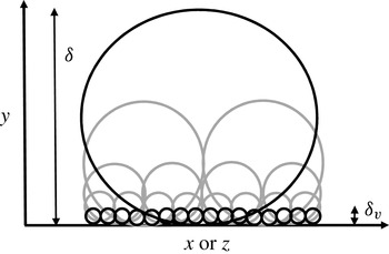
’ (the wall-normal direction) which allows one to asymptotically match between the law of the wall and the velocity defect law at high Reynolds numbers (Millikan Reference Millikan1938). Townsend (Reference Townsend1961, Reference Townsend1976) deduced that it would be difficult to explain this feature unless the size of the energy-containing motions (i.e. coherent structures) in the logarithmic region is proportional to distance of their centres from the wall. The energy-containing motions in the logarithmic region would therefore extend to the wall, and, in this sense, they are ‘attached’ to the wall. Furthermore, since the size of each of the energy-containing motions is determined by its wall-normal location, this implies that energy-containing motions in wall-bounded turbulence would be structured in a hierarchical form as described in Perry & Chong (Reference Perry and Chong1982) (see also the conceptual sketch in figure 1).
This insightful observation led Townsend (Reference Townsend1976) to develop a theory which predicts turbulence intensities in the logarithmic region. By assuming that each individual energy-containing motion (i.e. single attached eddy) is self-similar with respect to its centre location
 $y=y_{a}$
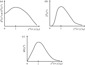
, he postulated that the statistical structure of an individual attached eddy would be as given in figure 2. Here, the key feature of the attached eddy is that its streamwise and spanwise components are non-negligibly large in the region close to the wall (figure 2
a) whereas the wall-normal component and Reynolds stress are very small (figure 2
b,c). It should be emphasised that this feature must be generic in wall-bounded flows, as it is a consequence of the presence of the ‘wall’ (i.e. impermeability condition): for example, in the original theory which neglects the viscous inner region, the wall-parallel components were assumed to satisfy the ‘slip’ boundary condition at the wall (figure 2
a), while the wall-normal component was set to ‘zero’, resulting in ‘zero’ Reynolds stress as well (figure 2
b,c). Superposing many of the self-similar attached eddies with a probability density function yielding constant Reynolds stress in the logarithmic region then leads to the following turbulence intensities:
 $$\begin{eqnarray}\displaystyle & \displaystyle \frac{\overline{u^{2}}}{u_{{\it\tau}}^{2}}=A_{1}-B_{1}\log \left(\frac{y}{L_{0}}\right), & \displaystyle\end{eqnarray}$$
 $$\begin{eqnarray}\displaystyle & \displaystyle \frac{\overline{w^{2}}}{u_{{\it\tau}}^{2}}=A_{2}-B_{2}\log \left(\frac{y}{L_{0}}\right), & \displaystyle\end{eqnarray}$$
 $$\begin{eqnarray}\displaystyle \frac{\overline{v^{2}}}{u_{{\it\tau}}^{2}}=A_{3},\quad \frac{\overline{uv}}{u_{{\it\tau}}^{2}}=A_{4},\end{eqnarray}$$
 $u$
,
 $v$
and
 $w$
are the streamwise, wall-normal and spanwise velocity fluctuations, respectively,
 $A_{i}~(i=1,2,3,4)$
and
 $B_{j}~(j=1,2)$
are constants,
 $u_{{\it\tau}}$
is the friction velocity, and
 $L_{0}$
is the upper limit of the wall-normal location that the attached eddies populate. Here, it should be mentioned that the logarithmic terms in (1.1a
,
b
) are an important result of the theory, which mathematically originate from the non-negligibly large contribution made by the streamwise and spanwise components of individual attached eddies close to the wall (figure 2
a). In contrast, the wall-normal intensity and the Reynolds stress do not show such logarithmic terms as their contributions to the region close to the wall are negligibly small (figure 2
b,c).
A schematic illustration of the attached-eddy hypothesis (Townsend Reference Townsend1976; Perry & Chong Reference Perry and Chong1982). Each of the circles indicates an individual attached eddy. The smallest eddy should scale in the inner length scale
 ${\it\delta}_{{\it\nu}}={\it\nu}/u_{{\it\tau}}$
(
 ${\it\nu}$
is kinematic viscosity and
 $u_{{\it\tau}}$
the friction velocity) whereas the largest one scales in the outer length scale
 ${\it\delta}$
. The size of the eddies in the logarithmic region (shown in grey) is proportional to the distance of their centres from the wall (i.e.
 $y$
), filling in the length scale separation between
 ${\it\delta}_{{\it\nu}}$
and
 ${\it\delta}$
. Note that this is merely a conceptual sketch, thus the population distribution of the attached eddies at each of the wall-normal locations is not intended to accurately represent that given in e.g. Perry & Chong (Reference Perry and Chong1982).

Second-order statistical moments of a single attached eddy (Townsend Reference Townsend1976): (a) streamwise and spanwise components; (b) wall-normal component; (c) Reynolds stress. Here,
 $y_{a}$
is the location where the attached eddy shows the maximum intensity. Sketch only.

The original theory of Townsend (Reference Townsend1976) has been significantly extended by Perry and coworkers, who further predicted and also verified the emergence of
 $k_{x}^{-1}$
spectra (
 $k_{x}$
is the streamwise wavenumber) through a series of refining works (Perry & Chong Reference Perry and Chong1982; Perry, Henbest & Chong Reference Perry, Henbest and Chong1986; Perry & Marusic Reference Perry and Marusic1995; Nickels et al.
Reference Nickels, Marusic, Hafez and Chong2005). Furthermore, during the last decade, a growing body of evidence which supports the attached-eddy hypothesis has emerged with rapidly growing computational power and experimental facilities with more advanced measurement techniques. The logarithmic growth of the near-wall streamwise turbulence intensity with the Reynolds number (De Graaff & Eaton Reference De Graaff and Eaton2000; Metzger & Klewicki Reference Metzger and Klewicki2001) has been understood as an example of this, as extending (1.1a
) to the near-wall region would give
 $\overline{u^{2}}\sim u_{{\it\tau}}^{2}\log Re_{{\it\tau}}$
(
 $\mathit{Re}_{{\it\tau}}$
is the friction Reynolds number) (Marusic & Kunkel Reference Marusic and Kunkel2003). More importantly, recent measurements from numerical and laboratory experiments have confirmed that (1.1) indeed appears when the Reynolds number is sufficiently high (Jiménez & Hoyas Reference Jiménez and Hoyas2008; Marusic et al.
Reference Marusic, Monty, Hultmark and Smits2013). Given such emerging statistical evidence, it is now likely that the energy-containing motions in wall-bounded turbulent flows exist in the form of attached eddies. Nevertheless, the essential question, namely what the single attached eddy really is, which constitutes the core of the original theory, has not been answered, remaining an issue of current debate. In the early studies, the form of an individual attached eddy was modelled in a statistical manner with the measurement data available: for example, Townsend (Reference Townsend1976) himself proposed a double-cone vortex as a model of single attached eddy by taking the experimental observations on the near-wall streaks (Kline et al.
Reference Kline, Reynolds, Schraub and Runstadler1967), whereas Perry & Chong (Reference Perry and Chong1982) and Perry et al. (Reference Perry, Henbest and Chong1986) modelled it as a ‘
 ${\it\Lambda}$
’-vortex from the observations by Head & Bandyopadhay (Reference Head and Bandyopadhay1981) who visualised the appearance of such vortices in a turbulent boundary layer.
Given the multi-scale nature of the eddies in wall-bounded flows, identifying the individual attached eddies and understanding their dynamical behaviour are very difficult to tackle even with modern measurement techniques and data from direct numerical simulations (DNS), placing these issues in the middle of current debate; the reader may also refer to two recent reviews by Adrian (Reference Adrian2007) and Jiménez (Reference Jiménez2013a ) which respectively reveal different viewpoints on the energy-containing motions in wall-bounded turbulent flows. Despite this debate, in recent years it has been suggested that the nature of the outer process is independent of the near-wall process. This feature has been reported by several recent studies, which showed that disturbing the near-wall region by wall roughness does not yield any significant change in the dynamics and statistics of the outer region (Flores & Jiménez Reference Flores and Jiménez2006; Flores, Jiménez & del Álamo Reference Flores, Jiménez and del Álamo2007; Hutchins & Marusic Reference Hutchins and Marusic2007; Lee, Sung & Krogstad Reference Lee, Sung and Krogstad2011). It is worth mentioning that this finding is seemingly contradictory to the early view in which the energy-containing motions in the outer region (e.g. the large-scale motions (LSMs)) were thought be an outcome of a bottom-up process e.g. via merger and growth of the near-wall hairpin vortices (Perry et al. Reference Perry, Henbest and Chong1986; Tomkins & Adrian Reference Tomkins and Adrian2003; Adrian Reference Adrian2007).
An alternative to this has been proposed by del Álamo et al. (Reference del Álamo, Jiménez, Zandonade and Moser2006), who argued that the process of energy-containing motions in the logarithmic and the wake outer regions is similar to that in the near-wall region. The near-wall process has been firmly understood in terms of the so-called ‘self-sustaining process’, which describes the interaction between the two predominant coherent structures, streaks and quasi-streamwise vortices (Hamilton, Kim & Waleffe Reference Hamilton, Kim and Waleffe1995; Waleffe Reference Waleffe1997; Jiménez & Pinelli Reference Jiménez and Pinelli1999; Schoppa & Hussain Reference Schoppa and Hussain2002). Streaks are significantly amplified by quasi-streamwise vortices via the ‘lift-up’ effect, the process transferring energy of mean shear to streamwise turbulent fluctuation (Landahl Reference Landahl1990; Butler & Farrell Reference Butler and Farrell1993). The amplified streaks then experience rapid oscillation caused by secondary instability or transient growth, which, in turn, generates new quasi-streamwise vortices via nonlinear mechanisms (Hamilton et al. Reference Hamilton, Kim and Waleffe1995; Schoppa & Hussain Reference Schoppa and Hussain2002). The near-wall process involving this cyclic dynamics has also been referred to as ‘bursting’ by coining the term from the early observations (Kline et al. Reference Kline, Reynolds, Schraub and Runstadler1967; Jiménez & Moin Reference Jiménez and Moin1991). del Álamo et al. (Reference del Álamo, Jiménez, Zandonade and Moser2006) suggested that such a process would also be possible in the logarithmic and the wake outer regions through similar interaction between the long streaky motions and the vortex packets observed in those regions. Indeed, Flores & Jiménez (Reference Flores and Jiménez2010) reported that the energy-containing motions in the logarithmic region exhibit an eddy turnover involving intense Reynolds stress generation, reminiscent of the bursting in the near-wall region.
The presence of self-sustaining processes above the near-wall region has also been supported by a number of recent theoretical studies, which examined the evolution of the organised part of a small perturbation driven by a flow field (del Álamo & Jiménez Reference del Álamo and Jiménez2006; Cossu, Pujals & Depardon Reference Cossu, Pujals and Depardon2009; Hwang & Cossu Reference Hwang and Cossu2010a
,Reference Hwang and Cossu
b
; Pujals et al.
Reference Pujals, García-Villalba, Cossu and Depardon2010; Willis, Hwang & Cossu Reference Willis, Hwang and Cossu2010). These studies showed that long streaky motions can be significantly amplified by the lift-up effect at all the length scales: i.e. the inner (
 ${\it\delta}_{{\it\nu}}\equiv {\it\nu}/u_{{\it\tau}}$
where
 ${\it\nu}$
is kinematic viscosity), logarithmic (
 $y$
) and outer (
 ${\it\delta}$
) scales. The amplification of the streaky motion scaling in the inner units appears at
 ${\it\lambda}_{z}^{+}\simeq 100$
, the spanwise spacing of the near-wall streaks (Kline et al.
Reference Kline, Reynolds, Schraub and Runstadler1967; Smith & Metzler Reference Smith and Metzler1983), while the one scaling in the outer units emerges at
 ${\it\lambda}_{z}\simeq O({\it\delta})$
, the spanwise spacing similar to that of very-large-scale motions (VLSMs), the long streaky structures in the outer region (Kim & Adrian Reference Kim and Adrian1999; del Álamo & Jiménez Reference del Álamo and Jiménez2003; Hutchins & Marusic Reference Hutchins and Marusic2007). It should be stressed that the streak amplification also appears at
 $100{\it\delta}_{{\it\nu}}<{\it\lambda}_{z}<O({\it\delta})$
and it mainly contributes to the logarithmic region (Hwang & Cossu Reference Hwang and Cossu2010b
). The amplified streaks in this case were found to be self-similar with respect to their spanwise size, reminiscent of Townsend’s attached eddies.
Very recently, more direct evidence on the presence of the self-sustaining process of the energy-containing motions in the logarithmic and the wake outer regions has been provided through a few numerical experiments (Hwang & Cossu Reference Hwang and Cossu2010c
, Reference Hwang and Cossu2011). It has been shown that the energy-containing motions at the outer scale (large-scale and very-large-scale motions) are able to be sustained even if the motions in the near-wall and the logarithmic regions are artificially removed (Hwang & Cossu Reference Hwang and Cossu2010c
). The same feature has also been found for the energy-carrying motions in the logarithmic region: i.e. the energy-carrying motions, the length scale of which is proportional to the distance from the wall, are able to be sustained in the absence of the motions at other length scales (Hwang & Cossu Reference Hwang and Cossu2011). It is very important to recall that the energy-containing motions at the length scale of the logarithm region (i.e.
 $y$
) are literally the attached eddies according to the definition by Townsend (Reference Townsend1976). Therefore, their self-sustaining nature implies that one would technically be able to isolate the ‘hypothetical’ attached eddies at a given length scale by artificially removing the motions at other scales, enabling one to directly access the entire statistical structure of the attached eddies at a given length scale.
Motivated by this observation, the goal of the present study is to compute the statistical structure of the self-sustaining attached eddies at a given length scale by performing a numerical experiment, in which the energy-containing motions only at the length scale are isolated by removing the motions at other scales. To achieve this goal, the numerical experiment is designed by combining two techniques introduced in our previous studies, one of which damps out the motions smaller than the given length scale through an over-damped large-eddy simulation (LES) (Hwang & Cossu Reference Hwang and Cossu2010c ) and the other removes the motions larger than that using an explicit filtering (Hwang Reference Hwang2013). We will see that the numerical experiment successfully isolates the attached eddies at a given length scale and results in a statistical structure for them consistent with that given by the original theory (Townsend Reference Townsend1976; Perry & Chong Reference Perry and Chong1982) (see also § 4), providing direct evidence on the existence of Townsend’s attached eddies.
This paper is organised as follows. We start by introducing the detailed methods of the present numerical experiment in § 2. The energy-containing motions at the outer scale are first studied in § 3 by extending the previous work performed at
 $\mathit{Re}_{{\it\tau}}=550$
(Hwang & Cossu Reference Hwang and Cossu2010c
) to
 $\mathit{Re}_{{\it\tau}}=955$
with the aim of providing a more complete form of the statistical structure of the self-sustaining outer motions. We then present the statistical structure of the isolated energy-containing motions at a given length scale in the logarithmic region (i.e. attached eddies) in § 4, where we also show that the statistical structure is self-similar with respect to the length scale. In § 5, a comprehensive discussion is presented by comparing the present results with the original theory and a number of previous findings. Here, special effort has been made to build a consistent description of the eddy structure of wall turbulence by integrating all the known coherent structures within the framework of the attached-eddy theory. This paper concludes in § 6 with a few remarks.
2. Numerical experiment
2.1. Large-eddy simulation
The numerical experiment in the present study is performed in a turbulent channel. We denote as
 $x$
,
 $y$
and
 $z$
the streamwise, wall-normal and spanwise directions, respectively. The height of the channel is chosen to be
 $2h$
, and its upper and lower walls are set to be located at
 $y=0$
and
 $y=2h$
, respectively. The numerical experiment in the present study is carried out using the Navier–Stokes solver which has also been verified through our previous studies (Hwang & Cossu Reference Hwang and Cossu2010c
, Reference Hwang and Cossu2011; Hwang Reference Hwang2013). In this solver, the streamwise and spanwise directions are discretised using the Fourier–Galerkin method with the
 $2/3$
rule for dealiasing, and the wall-normal direction is discretised using second-order central difference. The time integration is conducted semi-implicitly based on the fractional-step method (Kim & Moin Reference Kim and Moin1985). All the terms with wall-normal derivatives are implicitly advanced using the second-order Crank–Nicolson method, while the rest of the terms are explicitly integrated using a third-order low-storage Runge–Kutta method. All the computations in the present study are performed by imposing a constant mass flux across the channel.
As mentioned, the numerical experiment is designed based upon an over-damped LES, which plays a key role in removing the motions smaller than the given length scale. For this purpose, it is highly desirable to prevent any possible energy transfer from the modelled residual stress during the simulation. Therefore, as in Hwang & Cossu (Reference Hwang and Cossu2010c
, Reference Hwang and Cossu2011), we consider the static Smagorinsky model in which the residual stress tensor
 $\tilde{{\it\tau}}_{ij}~(i,j,k=1,2,3)$
is given as
 $$\begin{eqnarray}\tilde{{\it\tau}}_{ij}-\frac{{\it\delta}_{ij}}{3}\tilde{{\it\tau}}_{kk}=-2{\it\nu}_{t}\tilde{\unicode[STIX]{x1D61A}}_{ij},\end{eqnarray}$$
where
 $$\begin{eqnarray}{\it\nu}_{t}=(C_{s}\tilde{{\it\Delta}})^{2}\tilde{\mathscr{S}}\mathscr{D}.\end{eqnarray}$$
Here,
 $\tilde{\cdot }$
denotes the filtered quantity,
 $\unicode[STIX]{x1D61A}_{ij}$
the strain rate tensor,
 $C_{s}$
the Smagorinsky constant,
 $\tilde{{\it\Delta}}=(\tilde{{\it\Delta}}_{1}\tilde{{\it\Delta}}_{2}\tilde{{\it\Delta}}_{3})^{1/3}$
the nominal filter width,
 $\tilde{\mathscr{S}}=(2\tilde{\unicode[STIX]{x1D61A}}_{ij}\tilde{\unicode[STIX]{x1D61A}}_{ij})^{1/2}$
the
 $y^{+}/A^{+}$
norm of the strain rate tensor, and
 $\mathscr{D}=1-\exp [-(y^{+}/A^{+})^{3}]$
is the van Driest damping function introduced to enforce proper behaviour in the near-wall region (Härtel & Kleiser Reference Härtel and Kleiser1998). For the filter of the present LES, we apply the grid filter (the filter inherently given by the spatial discretisation): i.e. the cut-off filter in the streamwise and spanwise directions and the box filter in the wall-normal direction.
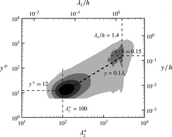
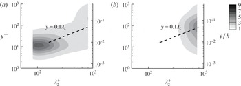
Premultiplied one-dimensional spanwise spectra of the streamwise velocity in turbulent channel flow at
 $\mathit{Re}_{{\it\tau}}=2003$
(from Hoyas & Jiménez Reference Hoyas and Jiménez2006). Here, the contour labels indicate 0.2, 0.4, 0.6 and 0.8 of the maximum, respectively.

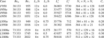
Simulation parameters in the present study. Here, the filtering (2.2) is applied to
 $L950a$
,
 $L950b$
,
 $L1800a$
,
 $L1800b$
and
 $L1800c$
, with the aim of simulating the isolated attached eddies at a given spanwise length scale
 ${\it\lambda}_{z,0}=L_{z}$
. In the names of the simulations,
 $F$
indicates ‘full’,
 $I$
‘intermediate’,
 $O$
‘outer’ and
 $L$
‘logarithmic’.

2.2. Computing attached eddies at a given length scale
Now, we design the numerical experiment which isolates the energy-containing motions at a given length scale. We first restrict the use of the definition of the attached eddy to the original one in Townsend (Reference Townsend1976) and Perry & Chong (Reference Perry and Chong1982): i.e. an attached eddy in the present study strictly refers to an energy-containing motion, the size of which is proportional to the distance from the wall. Throughout the present study, any other use of the term ‘attached’ is intentionally avoided so as not to generate any confusion. Given this definition, the design of the present numerical experiment should start by asking what statistically measurable quantity would characterise the length scale (or size) of the attached eddies. The key in answering this question can be found from previous findings where the spanwise length scale of energy-containing motions in the logarithmic region is shown to be linearly proportional to the distance from the wall (Tomkins & Adrian Reference Tomkins and Adrian2003; del Álamo et al.
Reference del Álamo, Jiménez, Zandonade and Moser2004; Ganapathisubramani et al.
Reference Ganapathisubramani, Hutchins, Hambleton, Longmire and Marusic2005; Hutchins, Hambleton & Marusic Reference Hutchins, Hambleton and Marusic2005). We note that recent investigations have shown that the local mixing length scale defined by
 $l(y)=u_{{\it\tau}}(\text{d}U/\text{d}y)^{-1}$
provides a better length scale for the logarithmic region (Mizuno & Jiménez Reference Mizuno and Jiménez2011; Pirozzoli Reference Pirozzoli2012), but this mixing length scale also gives the linear growth of the spanwise length scale at least at the leading-order, especially if the logarithmic behaviour becomes evident as for the flows at sufficiently high Reynolds numbers.
In figure 3, we show one-dimensional spanwise spectra of the streamwise velocity from DNS by Hoyas & Jiménez (Reference Hoyas and Jiménez2006). The spanwise spectra are aligned along a linear ridge
 $y\simeq 0.1{\it\lambda}_{z}$
throughout the logarithmic region, indicating the linear growth of the spanwise correlation length scale with the distance from the wall. At the bottom end of this ridge (
 $y^{+}=12$
and
 ${\it\lambda}_{z}^{+}=100$
), a local maximum, which characterises well the spanwise spacing of the well-known near-wall streaks and quasi-streamwise vortices, appears. On the other hand, at the top end (
 $y=0.15h$
and
 ${\it\lambda}_{z}=1.5h$
), another local maximum scaling in the outer units is present. As we shall see in § 3.2, the spanwise wavelength of this local maximum gives the spanwise length scale of both large-scale (Kovasznay, Kibens & Blackwelder Reference Kovasznay, Kibens and Blackwelder1970) and very-large-scale motions (Kim & Adrian Reference Kim and Adrian1999; del Álamo & Jiménez Reference del Álamo and Jiménez2003; Hutchins & Marusic Reference Hutchins and Marusic2007). The presence of the ridge
 $y=0.1{\it\lambda}_{z}$
connecting the two local maxima is a strong indication of the existence of the attached eddies, and also suggests that the size of each of the attached eddies would be characterised by its spanwise length scale.
The present numerical experiment has been built upon this observation, such that the energy-containing motions at a given spanwise length scale
 ${\it\lambda}_{z,0}$
in the range of the ridge
 $y=0.1{\it\lambda}_{z}$
are isolated by removing those at other scales. We first introduce how we remove the energy-containing motions, the spanwise size of which is larger than the given one (
 ${\it\lambda}_{z}>{\it\lambda}_{z,0}$
). Here, we adopt the approach given by our previous DNS-based work, in which the energy-containing motions at
 ${\it\lambda}_{z}^{+}\gtrsim 100$
are explicitly filtered out (Hwang Reference Hwang2013). From the given goal of the numerical experiment, it is unnecessary to resolve the motions at
 ${\it\lambda}_{z}>{\it\lambda}_{z,0}$
. Therefore, we first set the spanwise computational domain as
 $L_{z}={\it\lambda}_{z,0}$
while considering long streamwise domains
 $L_{x}=8{\rm\pi}\sim 12{\rm\pi}h$
(see also table 1). However, even with this kind of computational domain, the motions at
 ${\it\lambda}_{z}>{\it\lambda}_{z,0}$
would not be completely removed (Hwang Reference Hwang2013), as those uniform along the spanwise direction would still be resolved. Hwang (Reference Hwang2013) showed that such eddies can be removed by applying the following explicit filtering which acts on the right-hand side of the discretised momentum equation at each Runge–Kutta substep:
 $$\begin{eqnarray}\left.\begin{array}{@{}rcl@{}}\widehat{\text{RHS}}_{x}(y,k_{x}\neq 0,\,k_{z}=0)\, & =\, & 0,\\ \widehat{\text{RHS}}_{y}(y,k_{x}\neq 0,\,k_{z}=0)\, & =\, & 0,\end{array}\!\right\}\end{eqnarray}$$
where
 $\widehat{\cdot }$
denotes the Fourier-transformed state in the
 $x$
and
 $z$
directions,
 $\text{RHS}_{i}$
is the right-hand side of the
 $i$
-component of the discretized momentum equation, and
 $k_{x}$
and
 $k_{z}$
are the streamwise and spanwise wavenumbers, respectively. We note that no action is applied to
 $\widehat{\text{RHS}}_{z}$
, as the filtering (2.2) is intended to remove only the two-dimensional motions populating the
 $x-y$
plane. For further details on this filtering, the reader may refer to Hwang (Reference Hwang2013) where its use was verified for the near-wall motions at
 ${\it\lambda}_{z}^{+}\leqslant 100$
.
Once the motions at
 ${\it\lambda}_{z}>{\it\lambda}_{z,0}$
are filtered out, the motions at
 ${\it\lambda}_{z}<{\it\lambda}_{z,0}$
are removed. This has been conducted by following the approach in Hwang & Cossu (Reference Hwang and Cossu2010c
) and Hwang & Cossu (Reference Hwang and Cossu2011) where the motions smaller than the given spanwise length scale are damped out by increasing the Smagorinsky constant
 $C_{s}$
, which has also been known to act in the same way as increasing the filter width of LES (Mason & Cullen Reference Mason and Cullen1986). Here, we should note that this approach does not strongly depend on the choice of the eddy viscosity model (Hwang & Cossu Reference Hwang and Cossu2010c
, Reference Hwang and Cossu2011): the use of a different type of eddy viscosity has also been examined in our previous studies, and it does not yield any qualitative difference from the use of (2.1b
).
2.3. Preliminary test
The designed numerical experiment has been carefully examined with a preliminary test. The DNS part of the present numerical solver has been verified at
 $\mathit{Re}_{{\it\tau}}\simeq 180$
in Hwang (Reference Hwang2013) where the data from the present numerical solver show very good agreement with those from del Álamo et al. (Reference del Álamo, Jiménez, Zandonade and Moser2004) (for further details, the reader may refer to Hwang Reference Hwang2013). A reference simulation is first performed to verify the present LES (see also
 $F950$
in table 1). A large computational box (
 $L_{x}=12{\rm\pi}$
and
 $L_{z}=6h$
) is considered with
 $C_{s}=0.05$
, the value known to provide the best statistical fit to the DNS result (i.e. the best result from an a posteriori test; see also Härtel & Kleiser Reference Härtel and Kleiser1998). To properly resolve the near-wall motions, the streamwise and spanwise grid spacings are chosen as
 ${\it\Delta}_{x}^{+}=45$
and
 ${\it\Delta}_{z}^{+}=94$
, respectively (after dealiasing), with the smallest wall-normal grid spacing
 ${\it\Delta}_{y,min}^{+}=1.8$
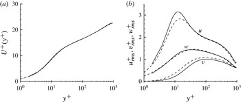
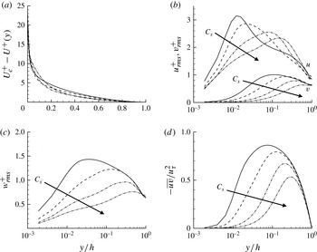
in the near-wall region (Zang Reference Zang1991). The computed mean-velocity profile and turbulent intensities are shown in figure 4. The mean-velocity profile is almost identical to that from DNS by del Álamo et al. (Reference del Álamo, Jiménez, Zandonade and Moser2004) (figure 4
a). The turbulent velocity fluctuations also agree reasonably well with those from the DNS except the streamwise one at
 $y^{+}\simeq 10{-}20$
; the streamwise velocity fluctuation at this location is a little larger than that of DNS (figure 4
b). It is worth mentioning that such a feature seems to be a general artifact which exists inherently in any LES of this kind, especially with a Smagorinsky-type model: for instance, the same feature has also been observed in a number of previous LES with Smagorinsky-type models (e.g. Germano et al.
Reference Germano, Piomelli, Moin and Cabot1991; Park et al.
Reference Park, Lee, Lee and Choi2006).
(a) Mean-velocity profile and (b) turbulent velocity fluctuations of the reference simulation: ——, present (
 $F950$
); - - - -, DNS at
 $\mathit{Re}_{{\it\tau}}=934$
(del Álamo et al.
Reference del Álamo, Jiménez, Zandonade and Moser2004).

Simulating the energy-containing motions only at a given spanwise length scale is then tested, and is illustrated with an example for
 ${\it\lambda}_{z,0}~(=L_{z})=0.5h~({\it\lambda}_{z,0}^{+}\simeq 900)$
. Figure 5(a) shows one-dimensional spanwise spectra of the streamwise velocity (
 $L1800b$
in table 1) after application of the narrow and long computational box with the filtering (2.2). It appears that the designed approach does indeed satisfactorily remove the motions wider than the given spanwise length, without significantly distorting the spectra aligned along the ridge
 $y=0.1{\it\lambda}_{z}$
. We then increase
 $C_{s}$
for removal of the motions at
 ${\it\lambda}_{z}<{\it\lambda}_{z,0}$
until the spectra exhibit a single well-defined peak at
 ${\it\lambda}_{z}\simeq {\it\lambda}_{z,0}$
. Here, it should be mentioned that the increase of
 $C_{s}$
does not significantly change
 $\mathit{Re}_{{\it\tau}}$
as in our previous studies (Hwang & Cossu Reference Hwang and Cossu2010c
, Reference Hwang and Cossu2011): for example,
 $\mathit{Re}_{{\it\tau}}=1644$
for
 $C_{s}=0.05$
and
 $\mathit{Re}_{{\it\tau}}=1745$
for
 $C_{s}=0.30$
in this case. One-dimensional spanwise spectra computed with the increased
 $C_{s}~(=0.30)$
are shown in figure 5(b). It now appears that the spectra of the streamwise velocity are concentrated only near
 ${\it\lambda}_{z}=L_{z}$
while maintaining the wall-normal peak location roughly on the ridge
 $y\simeq 0.1{\it\lambda}_{z}$
, indicating that only the energy-containing motions at
 ${\it\lambda}_{z}={\it\lambda}_{z,0}$
are left in the computational domain.
Here, it should also be mentioned that the spectral energy of the streamwise component of the isolated motions at the given spanwise length scale is found to be larger than that of the original one (compare figure 5
a with 5
b). Throughout the present study, this behaviour appears only in the streamwise velocity component (see also figure 8). A possible origin might be the nature of the Smagorinksy model itself which tends to over-predict the streamwise velocity fluctuation at its peak location compared to that of DNS (figure 4
b). However, the eddies isolated by this numerical experiment would not exhibit realistic interactions with the removed eddies. It is also difficult to neglect this effect, leaving the origin of this behaviour inconclusive. Lastly, it should also be mentioned that the wall-normal location of the peak at
 ${\it\lambda}_{z}=L_{z}$
for
 $C_{s}=0.3$
(figure 5
b) is also a little different from that for
 $C_{s}=0.05$
(figure 5
a), indicating that the removal of the motions smaller than
 ${\it\lambda}_{z}=L_{z}$
by increasing
 $C_{s}$
also slightly affects the motions that are to be isolated (see also figure 7).
Premultiplied one-dimensional spanwise spectra of streamwise velocity (
 $L1800b$
): (a)
 $C_{s}=0.05$
; (b)
 $C_{s}=0.30$
.

The designed numerical experiment has been performed by considering several different spanwise lengths and two different Reynolds numbers (
 $\mathit{Re}_{{\it\tau}}\simeq 950$
and
 $\mathit{Re}_{{\it\tau}}\simeq 1800$
). To save the computational cost in seeking appropriate
 $C_{s}$
values that will satisfactorily remove motions smaller than the given spanwise length scale, we first tested the
 $C_{s}$
values found in Hwang & Cossu (Reference Hwang and Cossu2011) with confined computational boxes of aspect ratio
 $L_{x}/L_{z}\simeq 0.5$
. In that study, the procedure to find the appropriate
 $C_{s}$
value was: (i) to set a computational box size; (ii) to increase the Smagorinsky constant from
 $C_{s}=0.05$
with an increment
 ${\rm\Delta}C_{s}=0.05$
; (iii) to select the largest
 $C_{s}$
which yields sustaining fluctuation in the flow field. It has been found that the use of the
 $C_{s}$
values in Hwang & Cossu (Reference Hwang and Cossu2011) also provides fairly good removal of the motions of spanwise size smaller than the given spanwise length scale, even in the present long computational boxes. The detailed parameters and the
 $C_{s}$
value for each of the present simulations are summarised in table 1. Here, we note that the chosen
 $C_{s}$
value tends to increase with the spanwise domain size
 $L_{z}$
. Given the definition of the Smagorinsky constant as in (2.1b
), the
 $C_{s}$
value would be viewed as a sort of filter width in the LES (see also Mason & Cullen Reference Mason and Cullen1986). Therefore, this behaviour simply indicates that bigger filter width (
 $C_{s}$
in this case) has to be used to remove larger motions.
3. Self-sustaining motions at the outer scale
For the purpose of completeness, we first study self-sustaining motions at the outer scale,
 ${\it\lambda}_{z}\simeq 1.5h$
, by extending the previous numerical experiment at
 $\mathit{Re}_{{\it\tau}}\simeq 550$
(Hwang & Cossu Reference Hwang and Cossu2010c
) to a higher Reynolds number
 $\mathit{Re}_{{\it\tau}}\simeq 950$
. In this case, one just needs to consider a sufficiently large computational box (i.e.
 $F950$
) and to simply increase
 $C_{s}$
until only the outer motions are left (Hwang & Cossu Reference Hwang and Cossu2010c
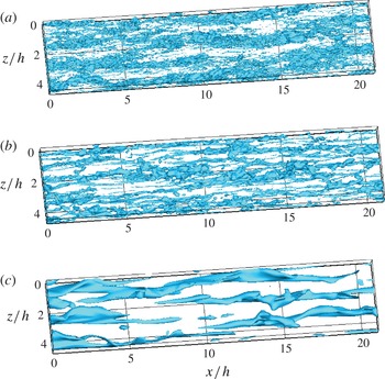
). Figure 6 shows instantaneous streamwise velocity fields on increasing
 $C_{s}~(=0.05,0.1,0.3)$
. The long streaky structures at the outer scale, referred to as VLSMs, are clearly visible in the reference simulation
 $F950~(C_{s}=0.05)$
with surrounding small-scale motions (figure 6
a). On increasing
 $C_{s}$
, the small-scale structures are gradually damped out (figure 6
b), and, at
 $C_{s}=0.3~(O950)$
, only the long streaky structures remain in the flow field (figure 6
c).
Isosurface of streamwise velocity fluctuation (
 $u^{+}=-2$
) on increasing
 $C_{s}$
: (a)
 $C_{s}=0.05~(F950)$
; (b)
 $C_{s}=0.10~(I950a)$
; (c)
 $C_{s}=0.30~(O950)$
.

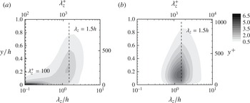
Premultiplied one-dimensional spanwise spectra of streamwise velocity: (a)
 $C_{s}=0.05~(F950)$
; (b)
 $C_{s}=0.30~(O950)$
. Here, the
 $y$
-axis is drawn with algebraic scale to better visualise spectra of the outer motions.

One-dimensional spanwise spectra shown in figure 7 also confirm the removal of the small-scale structures, especially the energy-containing ones in the near-wall and the logarithmic regions. For
 $C_{s}=0.05$
, the energy-containing motions are present at all the length scales (figure 7
a) as in DNS (figure 3). On the other hand, for
 $C_{s}=0.3$
, only the motions at
 ${\it\lambda}_{z}=1.5h$
are present (figure 7
b). It is also interesting to note that the shape of the spectra for
 $C_{s}=0.3$
in the
 ${\it\lambda}_{z}{-}y$
plane is not very different from that for
 $C_{s}=0.05$
, although the spectra for
 $C_{s}=0.3$
are more energetic than those for
 $C_{s}=0.05$
as discussed.
3.1. Mean velocity and turbulence intensities
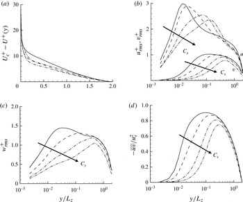
Figure 8 shows mean-velocity profile (the velocity defect law) and turbulent velocity fluctuations on increasing
 $C_{s}$
. As
 $C_{s}$
is increased, the mean-velocity profile experiences a non-trivial change over the entire wall-normal region except very outer region
 $y>0.6h$
(figure 8
a). Given the intensification of the streamwise velocity with the increase of
 $C_{s}$
discussed in § 2.3 (figure 5
b, see also figure 7
b), such a non-trivial change might have been expected. Here, it is worth mentioning the recent work by Tuerke & Jiménez (Reference Tuerke and Jiménez2013) who performed a numerical simulation with prescribed mean-velocity profiles. It might be possible to improve the present numerical experiment by taking such an approach to fix the distortion of the mean-velocity profile on increasing
 $C_{s}$
. However, one should also note that the non-trivial change of the mean-velocity profile on increasing
 $C_{s}$
also indicates the importance of the removed coherent structures in the generation of the mean-velocity profile. In this respect, it is also worth noting that the distortion of the mean-velocity profile does not appear to significantly affect the energy-containing motions that are to be isolated, as we shall see in § 3.2 that the length scales of the isolated outer motions in
 $O950$
are not very different from those of the outer motions in
 $F950$
.
Statistics with the increase of
 $C_{s}$
: (a) mean-velocity profile (
 $U_{c}^{+}$
is the centreline velocity); (b) streamwise and spanwise turbulent intensities; (c) wall-normal turbulent intensity; (d) Reynolds stress. Here, ——,
 $C_{s}=0.05~(F950)$
; - - - -,
 $C_{s}=0.10~(I950a)$
; – - – - –,
 $C_{s}=0.20~(I950b)$
; –
 $\cdot \cdot$
–
 $\cdot \cdot$
–;
 $C_{s}=0.30~(O950)$
.

In the case of the streamwise velocity fluctuation, the increase of
 $C_{s}$
does not yield a significant change for
 $y>0.6h$
as in the mean-velocity profile (figure 8
b). However, it significantly reduces the streamwise velocity fluctuation both in the near-wall (
 $y\lesssim 0.02h~(\simeq 20{\it\delta}_{v})$
in this case) and the logarithmic (
 $0.02h\lesssim y\lesssim 0.2h$
) regions (figure 8
b) although the peak value for a higher
 $C_{s}$
is larger than the value at the same wall-normal location for
 $C_{s}=0.05$
due to the feature explained in § 2.3. On the other hand, the wall-normal and spanwise velocity fluctuations exhibit simpler behaviour on increasing
 $C_{s}$
: they are damped out gradually from the near-wall region with the increase of
 $C_{s}$
, while maintaining good agreement in the regions sufficiently far from the wall (figure 8
b,c). The same feature has been found in the Reynolds stress on increasing
 $C_{s}$
: it is also gradually damped out from the near-wall region as
 $C_{s}$
is increased (figure 8
d). Given the fact that the Reynolds stress is correlation between the streamwise and wall-normal velocity fluctuations, this seems to indicate that the Reynolds stress is affected a little more by the wall-normal velocity fluctuation than by the streamwise one.
3.2. One-dimensional spectra
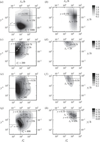
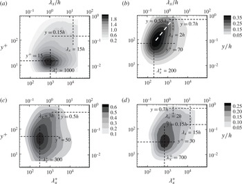
One-dimensional streamwise spectra of
 $O950~(C_{s}=0.30)$
are compared with those of the reference simulation
 $F950~(C_{s}=0.05)$
in figure 9. Here, we have chosen the spectra of
 $F950$
instead of those of DNS at
 $\mathit{Re}_{{\it\tau}}=934$
(del Álamo et al.
Reference del Álamo, Jiménez, Zandonade and Moser2004) for the comparison because the longer streamwise domain of
 $F950~(L_{x}\simeq 12{\rm\pi})$
appears to better visualise the spectra for
 ${\it\lambda}_{x}>5\sim 10h$
. The spectra of
 $F950$
also show reasonable agreement with those of the DNS:
 $F950$
fairly well predicts the peak locations in the spectra as well as the general shape in the outer region (see appendix A for further details).
Premultiplied one-dimensional streamwise spectra of (a,b) streamwise, (c,d) wall-normal, (e,f) spanwise velocities and (g,h) Reynolds stress: (a,c,e,g)
 $F950$
; (b,d,f,h)
 $O950$
.

The spectra of
 $F950$
depict well the coherent structures in the near-wall region. The near-wall peak in the streamwise velocity spectra at
 ${\it\lambda}_{x}^{+}\simeq 1000$
and
 $y^{+}\simeq 15$
(figure 9
a) indicates the near-wall streaks (e.g. Kline et al.
Reference Kline, Reynolds, Schraub and Runstadler1967) while the peaks in the wall-normal and the spanwise spectra around
 ${\it\lambda}_{x}^{+}\simeq 200$
and
 $y^{+}\simeq 50\sim 70$
(figure 9
c,e) characterise well the near-wall quasi-streamwise vortices (Kim, Moin & Moser Reference Kim, Moin and Moser1987; Jeong et al.
Reference Jeong, Benney, Schoppa and Kim1997; Hwang Reference Hwang2013), confirming the bimodal behaviour of the near-wall turbulent fluctuations (Jiménez, del Álamo & Flores Reference Jiménez, del Álamo and Flores2004; Hwang Reference Hwang2013): i.e. the long near-wall streaks, and the short and relatively isotropic vortical structures. Such a bimodal behaviour leads the near-wall Reynolds-stress spectra to exhibit their peak at
 ${\it\lambda}_{x}^{+}\simeq 700$
and
 $y^{+}\simeq 30$
, the location roughly between the regions of the two peaks respectively in the streamwise and the wall-normal velocity spectra (figure 9
g).
In the outer region (
 $y>0.15h$
), the spectra also appear to suggest the presence of two coherent structures, the LSMs and the VLSMs. As discussed in Monty et al. (Reference Monty, Hutchins, NG, Marusic and Chong2009), the LSMs would be depicted by the protruded part of the streamwise velocity spectra roughly at
 ${\it\lambda}_{x}\simeq 2\sim 3h$
and
 $y>0.4h$
(figure 9
a) where the wall-normal and spanwise velocity spectra also show significant amounts of energy (figure 9
c,e). On the other hand, the VLSMs are seen to be characterised by the intense energy at
 ${\it\lambda}_{x}^{+}\simeq 15h$
and
 $y\simeq 0.15h$
in the streamwise velocity spectra (figure 9
a). We note that the wall-normal and spanwise velocity spectra at this location exhibit lower energy than the streamwise ones (figure 9
c,e). Especially, the amount of energy in the wall-normal velocity spectra is very small (figure 9
c) even compared to that in the spanwise velocity spectra which contain at least some energy. The Reynolds stress is largest in the region between the locations of the two peaks respectively related to LSMs (
 ${\it\lambda}_{x}\simeq 2\sim 3h$
and
 $y\simeq 0.5\sim 0.7h$
) and VLSMs (
 ${\it\lambda}_{x}^{+}\simeq 15h$
and
 $y=0.15h$
) (figure 9
g). Finally, it should be pointed out that, unlike the spanwise spectra which rather clearly reveal a ridge indicating the linear growth of the correlation length scale with
 $y$
(e.g. figure 3), such a ridge is not evident in the streamwise spectra, except those for wall-normal velocity such a ridge is relatively easily seen along
 $y\simeq 0.35{\it\lambda}_{x}$
(figures 9
c and 14
b below for the spectra of DNS). This issue will be discussed further in § 5.2.
Now, we compare the spectra of
 $F950$
with those of
 $O950$
obtained only with the motions at
 ${\it\lambda}_{z}\simeq 1.5h$
(figure 7). Given the crudeness of the artificial eddy viscosity with a high
 $C_{s}$
for removal of the small-scale motions, the spectra of
 $O950$
seem to fairly well represent the outer part of
 $F950$
although the spectra of
 $O950$
are more intense and a little longer than those of
 $F950$
in the outer region. In particular, the locations of the outer peaks appear to be almost identical to those in the outer spectra of
 $F950$
(compare figures 9
a,c,e,g respectively with 9
b,d,f,h). The spectra of
 $O950$
now more clearly reveal the bimodal behaviour of the outer motions: the intense energy at
 ${\it\lambda}_{x}\simeq 2\sim 3h$
and
 $y=0.5\sim 0.7h$
in the spectra of all the velocity components (figure 9
b,d,f,h) represent the LSMs, whereas the peak in the streamwise velocity spectra at
 ${\it\lambda}_{x}\simeq 15h$
and
 $y\simeq 0.15h$
indicates the VLSMs (figure 9
b).
The spectra of
 $O950$
also indicate that the VLSMs tend to penetrate deep into the near-wall region: the streamwise energy of
 $O950$
at
 ${\it\lambda}_{x}\simeq 15h$
prevails over the entire logarithmic region, reaching even
 $y^{+}=10$
(figure 9
b). We note that such a feature also appears in the streamwise velocity spectra of
 $F950$
(figure 9
a): for
 ${\it\lambda}_{x}\simeq 15h$
, the energy in the streamwise velocity spectra of
 $F950$
is also fairly strong at
 $y^{+}=10$
. This is consistent with a number of recent findings which reported the influence of the outer structures in the logarithmic and the near-wall regions (Tomkins & Adrian Reference Tomkins and Adrian2005; Hoyas & Jiménez Reference Hoyas and Jiménez2006; Hutchins & Marusic Reference Hutchins and Marusic2007; Mathis, Hutchins & Marusic Reference Mathis, Hutchins and Marusic2009; Talluru et al.
Reference Talluru, Baidya, Hutchins and Marusic2014). Since the wall-normal velocity fluctuation is very small in the region close to the wall (figure 9
d), the penetration of the streamwise velocity fluctuation at long wavelength would require some spanwise velocity fluctuation due to continuity, and this is indeed seen in the spectra of spanwise velocity (i.e.
 $y^{+}\leqslant 100$
in figure 9
f; see also figure 8
c where
 $w_{rms}^{+}$
of
 $O950$
at
 $y=0.5h~(y^{+}\simeq 53)$
is still approximately one third of that of
 $F950$
). Finally, the very small wall-normal velocity fluctuation below
 $y\simeq 0.1h$
does not allow the Reynolds stress spectra of
 $O950$
to reach below
 $y\simeq 0.05h$
, indicating that the VLSMs in this region carry very little Reynolds stress (see also § 5.3 for further discussion).
3.3. Instantaneous flow field
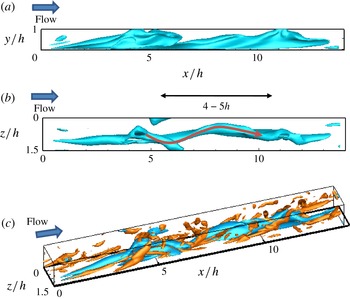
As shown in figure 6, the streamwise velocity field of
 $O950$
is characterised by long streaky structures. A detailed flow field around a single streaky structure is visualised in figure 10. The side view shows that the streaky structure is connected through the region relatively close to the wall (
 $y\lesssim 0.2h$
) (figure 10
a), and its length roughly extends to
 ${\it\lambda}_{x}\simeq 10\simeq 15h$
, corresponding to the peak in the streamwise spectra at
 ${\it\lambda}_{x}\simeq 15h$
and
 $y\simeq 0.15h$
(figure 9
b). Above
 $y\simeq 0.2h\sim 0.3h$
, the streaky structure tends to be inclined to the wall, as also found in recent experiments (e.g. Dennis & Nikels Reference Dennis and Nikels2011a
,Reference Dennis and Nikels
b
). The top view suggests that this behaviour seems to be linked to the meandering nature of each of the streaky structures reported by Hutchins & Marusic (Reference Hutchins and Marusic2007) (figure 10
b). The dominant vortical structures appear in the form of quasi-streamwise vortices, and they are found to be aligned along the streaky structure (figure 10
c). Vortices at the crest of the streaky structure (
 $(x,y)\simeq (5h,1h)$
and
 $(x,y)\simeq (11h,1h)$
in figure 10
c) are found to be rather disorganised, and it is difficult to view them as arc-like vortices, at least with instantaneous flow fields. The inclination of the streaky structure and the quasi-streamwise vortices aligned to that appear with the streamwise spacing
 ${\it\lambda}_{x}\simeq 3\sim 5h$
, suggesting that they are an LSM in the
 $O950$
simulation, yielding the intense energy at
 ${\it\lambda}_{x}\simeq 2\sim 4h$
and
 $y>0.4h$
in the streamwise spectra of all the velocity components of
 $O950$
(figure 9
b,d,f,h).
Instantaneous velocity field around a single streaky structure (VLSM) from
 $O950$
: (a) side view; (b) top view; (c) perspective view. Here, the blue isosurfaces indicate
 $u^{+}=-2.45$
, and, in (c), the orange isosurfaces represent the second invariant of the velocity gradient tensor with
 $Q=0.5\times 10^{-4}u_{{\it\tau}}^{4}/{\it\nu}^{2}$
.

4. Self-sustaining attached eddies in the logarithmic region
Now, we consider energy-containing motions, the spanwise length scale of which is proportional to the distance from the wall: i.e.
 ${\it\lambda}_{z}\sim y$
. As discussed in detail in § 2, we isolate the energy-containing motions at a given spanwise length scale
 ${\it\lambda}_{z,0}=L_{z}$
by removing the motions at other length scales. The behaviour of the wall-normal profiles of the first- and second-order statistics on increasing
 $C_{s}$
in this case is reported in appendix B.
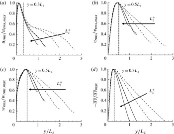
Normalised second-order statistics of the motions rescaled with the given spanwise length
 $L_{z}$
: (a) streamwise velocity; (b) wall-normal velocity; (c) spanwise velocity; (d) Reynolds stress. Here, ——,
 $\mathit{Re}_{{\it\tau}}\simeq 950$
(
 $L950a$
,
 $L950b$
); - - - -,
 $\mathit{Re}_{{\it\tau}}\simeq 1800$
(
 $L1800a$
,
 $L1800b$
,
 $L1800c$
).

4.1. Turbulence intensities
Figure 11 shows velocity fluctuations of the isolated motions at a given spanwise length scale. Here, each of the velocity fluctuations is normalised with its peak value, and the wall-normal coordinate is rescaled with the spanwise length scale,
 ${\it\lambda}_{z,0}(=L_{z})$
(table 1). All of the velocity fluctuations are found to be self-similar with the spanwise length scale
 $L_{z}$
below certain wall-normal locations: the streamwise velocity fluctuation and the Reynolds stress are self-similar for
 $y\leqslant 0.3L_{z}$
(figure 11
a,d), and the wall-normal and spanwise velocity fluctuations show the same behaviour for
 $y\leqslant 0.5L_{z}$
(figure 11
b,c). Above these wall-normal locations, they do not bear such self-similarity. However, as we shall see in the one-dimensional spectra (§ 4.2), the non-self-similar part is the fluctuation induced by the self-similar part, at the wall-normal locations supposed to be ‘empty’ due to the absence of the motions at
 ${\it\lambda}_{z}>L_{z}$
: i.e. the non-self-similar part does not originate from a physical process at different length scale. In this respect, it is worth noting that the peak location in the one-dimensional spectra of the non-self-similar part is found to be the same as that of the self-similar part located closer to the wall. It is also worth mentioning that the same behaviour has been found in our previous numerical experiment (Hwang Reference Hwang2013) where the motions at
 ${\it\lambda}_{z}^{+}>100$
are removed with the same filtering technique.
Given the observation that the spanwise spectra are aligned along the ridge
 ${\it\lambda}_{z}\sim y$
(e.g. figures 3 and 5), the emergence of the self-similarity with respect to the spanwise length scale
 $L_{z}$
in figure 11 indicates that the size of the isolated energy-containing motions at each of the spanwise length scales is proportional to the distance from the wall. More importantly, the self-similar part of the velocity fluctuations is remarkably similar to the second-order statistical moments generated by a single attached eddy in the original hypothesis (compare figure 11 with 2): the streamwise and the spanwise velocity fluctuations clearly show non-negligible amounts of energy close to the wall (
 $y<0.05L_{z}$
in figure 11
a,c), whereas the wall-normal velocity fluctuation and the Reynolds stress are considerably smaller in that region (figure 11
b,d). Given the fact that this feature is also only physically reasonable and kinematically admissible behaviour due to the presence of the wall, this should not be surprising, although it is an essential ingredient to reach the prediction given in (1.1). The only important difference from the sketch in figure 2 is that the peak location of the computed streamwise velocity fluctuation in the present study (
 $y\simeq 0.1L_{z}$
; figure 11
a) is not the same as that of the wall-normal and the spanwise velocity fluctuations (
 $y\simeq 0.4\sim 0.5L_{z}$
; figure 11
b,c) unlike the original hypothesis (figure 2). Apart from this, the computed second-order statistical moments suggest that each of the energy-containing motions at a given spanwise length scale exactly fits the definition of the attached eddy given by Townsend (Reference Townsend1976) and Perry & Chong (Reference Perry and Chong1982), suggesting that they are the attached eddies (see also a further discussion in § 5).
4.2. One-dimensional spectra
One-dimensional spectra of the isolated energy-containing motions at a given spanwise length scale are shown in figure 12 for several
 $L_{z}$
. It might be difficult to see that the entire structure of the spectra is self-similar with the spanwise length scale
 $L_{z}$
, but, at least, the peak locations in the spectra appear to be self-similar with
 $L_{z}$
. The spectra of the streamwise velocity show the maximum at
 ${\it\lambda}_{x}\simeq 10L_{z}$
and
 $y\simeq 0.1L_{z}$
, explaining why the peak of the streamwise velocity fluctuation appears at
 $y\simeq 0.1L_{z}$
unlike the other components (figure 11
a). We note that the emergence of this peak in the streamwise spectra (figure 11
a) can also be justified as the spanwise spectra of the full simulation are aligned along the ridge
 $y\simeq 0.1{\it\lambda}_{z}$
(figure 2). The spectra of wall-normal and spanwise velocities exhibit their maximum roughly at the same location,
 ${\it\lambda}_{x}\simeq 3L_{z}$
and
 $y\simeq 0.5L_{z}$
(figure 11
b,c), where the streamwise velocity spectra also show a non-negligible amount of energy (figure 11
a).
Premultiplied one-dimensional streamwise spectra of (a) streamwise, (b) wall-normal, (c) spanwise velocities and (d) Reynolds stress. Here, the solid, dashed and shaded contours indicate
 $L1800a$
,
 $L1800b$
and
 $L1800c$
, respectively. The contour levels are chosen as 0.25, 0.5 and 0.75 times each of the maximum for comparison.

The velocity spectra suggest that the energy-containing motions at a given spanwise length scale would also be characterised by two types of structure: one is a long streaky structure carrying intense streamwise turbulent kinetic energy (
 ${\it\lambda}_{x}\simeq 10L_{z}$
and
 $y\simeq 0.1L_{z}$
), and the other is a short and tall vortex packet which contains all the velocity components (
 ${\it\lambda}_{x}\simeq 3L_{z}$
and
 $y\simeq 0.5L_{z}$
). This bimodal behaviour also leads the energetic region in the Reynolds stress spectra to be placed in the region between the locations of the two peaks respectively associated with the two structures (figure 11
d). The spectra also indicate that the long mode reaches deep into the region close to the wall (figure 12
a): the spectra of streamwise velocity at
 ${\it\lambda}_{x}\simeq 10L_{z}$
are very energetic for
 $y<0.1L_{z}$
. In contrast, the spectra of wall-normal velocity exhibit little energy below
 $y\simeq 0.1L_{z}$
(figure 12
b), explaining the very small amount of Reynolds stress for
 $y<0.1L_{z}$
(figure 12
d; see also a further discussion in § 5.3). This feature also appears to yield a considerable amount of the spanwise velocity fluctuation below
 $y\simeq 0.1L_{z}$
due to continuity.
4.3. Instantaneous flow field
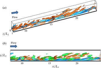
The instantaneous flow field of the isolated energy-containing motions at a given spanwise length scale is also visualised in figure 13. As expected from the discussion on the spectra (figure 12), the flow field exhibits long streaky structures (blue isosurfaces in figure 13) and relatively short vortical structures (orange isosurfaces in figure 13). In particular, the vortical structures are seen to be aligned along the streaky structures that extend to roughly
 ${\it\lambda}_{x}\simeq 10L_{z}$
. However, as in the outer motions (figure 10), it is difficult to find well-defined arc-like vortices, at least in instantaneous flow fields. It appears that the vortical structures are also highly correlated with the wall-normal velocity fluctuations (green isosurfaces in figure 13
b), suggesting that the vortical structure would be represented well by the wall-normal velocity fluctuations, the streamwise length scale of which is
 ${\it\lambda}_{x}\simeq 2\sim 4L_{z}$
(figure 12
b). The wall-normal location of the peak of the wall-normal velocity fluctuations implies that the vortical structures would be viewed as ‘tall’, especially compared to the wall-normal location of the streaky structure represented by the streamwise velocity fluctuations (see also figure 12
a,b).
Instantaneous velocity field around a single streaky structure (
 $L1800b$
): (a) perspective and (b) side views. Here, the blue isosurfaces indicate
 $u^{+}=-2.5$
, the green ones
 $v^{+}=-0.095$
, and the orange ones the second invariant of the velocity gradient tensor
 $Q=1.1\times 10^{-4}u_{{\it\tau}}^{4}/{\it\nu}^{2}$
.

5. Discussion
Thus far, we have performed a set of numerical experiments by which only the energy-containing motions at a given spanwise length scale are isolated. The spanwise length scales considered in the present study are
 ${\it\lambda}_{z}^{+}>100$
, thus the present study basically extends our recent work, in which the near-wall energy-containing motions at
 ${\it\lambda}_{z}^{+}\leqslant 100$
are isolated (Hwang Reference Hwang2013), to the logarithmic and the wake outer regions. The successful isolation of energy-containing motions at a give spanwise length scale suggests that they have their own self-sustaining mechanism essentially independent of the motions at other scales, confirming the previous conclusion in Hwang & Cossu (Reference Hwang and Cossu2010c
) and Hwang & Cossu (Reference Hwang and Cossu2011) as well as the findings in recent studies where the outer turbulence is found to be independent of disruption of the near-wall process by roughness on the wall (Flores & Jiménez Reference Flores and Jiménez2006; Flores et al.
Reference Flores, Jiménez and del Álamo2007; Hutchins & Marusic Reference Hutchins and Marusic2007; Lee et al.
Reference Lee, Sung and Krogstad2011; Chung, Monty & Ooi Reference Chung, Monty and Ooi2014).
Probably the most important finding in the present study is that the computed statistical structure of the isolated energy-containing motions at each of the spanwise length scales is self-similar with the spanwise length (figures 11 and 12). Since the spanwise length scale is proportional to distance from the wall (figure 3), this indicates that the size of these motions is proportional to the distance from the wall. Furthermore, the second-order statistical moments computed in the present study (figure 11) are found to resemble the statistical properties of the attached eddies at a given length scale in the original hypothesis (figure 2): the streamwise and spanwise components have non-negligible contributions to the region close to the wall (figure 11
a,c), whereas the wall-normal component and the Reynolds stress are considerably smaller in that region (figure 11
b,d). These findings suggest that the isolated energy-containing motions at a given spanwise length scale are the ‘attached eddies’ which Townsend (Reference Townsend1976) and Perry & Chong (Reference Perry and Chong1982) have foreseen. The existence of the attached eddies therefore directly supports all of the previous contributions along this line: i.e. the emergence of
 $k_{x}^{-1}$
spectra (see also § 5.2; Perry & Chong Reference Perry and Chong1982; Perry et al.
Reference Perry, Henbest and Chong1986; Perry & Marusic Reference Perry and Marusic1995; Nickels et al.
Reference Nickels, Marusic, Hafez and Chong2005), the logarithmic growth of the near-wall turbulence intensity with the Reynolds number (Marusic & Kunkel Reference Marusic and Kunkel2003), and the logarithmic wall-normal dependence on the second- and higher-order statistical moments of the wall-parallel velocity components (Perry & Chong Reference Perry and Chong1982; Jiménez & Hoyas Reference Jiménez and Hoyas2008; Marusic et al.
Reference Marusic, Monty, Hultmark and Smits2013; Meneveau & Marusic Reference Meneveau and Marusic2013).
Finally, it is worth mentioning that the self-similarity found in the present study is the outcome of the ‘self-sustaining nature’ of the motions at a given spanwise length scale. Given the nature of the present numerical experiment which constrains the spanwise length scale of the resolved motions, the self-similarity may also be able to be obtained with a DNS (e.g. spectra, conditional structure, etc.). However, in that case, it does not necessarily imply that the motions at a given spanwise length scale would be able to be sustained by themselves, unlike the conclusion reached in the present study. In this respect, it is now important to carefully examine if the self-similar motions found in the present study would indeed be observed in the previous statistical data from laboratory experiments or DNS. We shall proceed with our discussion from this point, as will be detailed in §§ 5.1 and 5.2.
5.1. The attached eddies
The one-dimensional spectra in figure 12 suggest that the energy-containing motions at a given spanwise length scale are composed of two distinct components: one is a long streaky structure mainly carrying streamwise turbulent kinetic energy and the other is a short and tall vortex packet carrying turbulent kinetic energy at all the velocity components. The size and the geometry of the former are roughly represented by (figure 12 a)
 $$\begin{eqnarray}y\simeq 0.1{\it\lambda}_{z}\quad \text{and}\quad {\it\lambda}_{x}\simeq 10{\it\lambda}_{z},\end{eqnarray}$$
whereas those of the latter are given by (figure 12 a–c)
 $$\begin{eqnarray}y\simeq 0.5\sim 0.7{\it\lambda}_{z}\quad \text{and}\quad {\it\lambda}_{x}\simeq 2\sim 3{\it\lambda}_{z}.\end{eqnarray}$$
Here, it should be emphasised that the two of them always appear together: i.e. there is no occasion when only one of them exists throughout the present numerical experiment. This suggests that it would be appropriate to interpret them as two dynamically interconnected elements of a single attached eddy, which generates the statistical structure given in § 4, rather than two different classes of attached eddies.
The former streaky structure appears be the low-momentum zone of the streamwise velocity observed in several previous studies (Ganapathisubramani, Longmire & Marusic Reference Ganapathisubramani, Longmire and Marusic2003; Tomkins & Adrian Reference Tomkins and Adrian2003; Hutchins et al.
Reference Hutchins, Hambleton and Marusic2005; del Álamo et al.
Reference del Álamo, Jiménez, Zandonade and Moser2006). However, the considerably long streamwise length (i.e.
 ${\it\lambda}_{x}\simeq 10{\it\lambda}_{z}$
) has not been much discussed, except by del Álamo et al. (Reference del Álamo, Jiménez, Zandonade and Moser2006) who showed the presence of such long streaky structures using a self-similar conditional average. In this respect, it is also worth mentioning the work by Kim & Adrian (Reference Kim and Adrian1999) who proposed that the vortical structures involving the low-momentum zone appear to be aligned in a coherent manner, resulting in a much longer structure. The presence of the long self-similar streaky structure given by (5.1a,b
) is therefore consistent with these previous findings.
The latter short and tall vortex packet has been better studied (Ganapathisubramani et al.
Reference Ganapathisubramani, Longmire and Marusic2003; Tomkins & Adrian Reference Tomkins and Adrian2003; Hutchins et al.
Reference Hutchins, Hambleton and Marusic2005; del Álamo et al.
Reference del Álamo, Jiménez, Zandonade and Moser2006). The aspect ratio (i.e.
 ${\it\lambda}_{x}\simeq 2\sim 3{\it\lambda}_{z}$
) and the nature in carrying all the velocity components suggest that it would be the vortical structure often referred to as either a ‘hairpin vortex packet’ (e.g. Ganapathisubramani et al.
Reference Ganapathisubramani, Longmire and Marusic2003; Tomkins & Adrian Reference Tomkins and Adrian2003; Hutchins et al.
Reference Hutchins, Hambleton and Marusic2005) or a ‘tall attached vortex cluster’ (e.g. del Álamo et al.
Reference del Álamo, Jiménez, Zandonade and Moser2006). It has been shown that the conditional structure of such vortical structures contains counter-rotating streamwise vortices (Hutchins et al.
Reference Hutchins, Hambleton and Marusic2005; del Álamo et al.
Reference del Álamo, Jiménez, Zandonade and Moser2006), and this is consistent with the instantaneous velocity field in the present study where the quasi-streamwise vortices are found (figure 13).
More physical insight is also gained by examining (5.1a,b
) and (5.1c,d
) further. The smallest spanwise length scale possible should be
 ${\it\lambda}_{z}^{+}\simeq 100$
which represents the spanwise length of the near-wall motions (figure 3). At this spanwise length, (5.1a,b
) and (5.1c,d
) respectively give
 $$\begin{eqnarray}y^{+}\simeq 10\quad \text{and}\quad {\it\lambda}_{x}^{+}\simeq 1000,\end{eqnarray}$$
 $$\begin{eqnarray}y^{+}\simeq 50\sim 70\quad \text{and}\quad {\it\lambda}_{x}^{+}\simeq 200\sim 300.\end{eqnarray}$$
It now becomes apparent that (5.2a,b
) indicate the well-known near-wall streaks (Kline et al.
Reference Kline, Reynolds, Schraub and Runstadler1967) while (5.2c,d
) are the quasi-streamwise vortices (Jeong et al.
Reference Jeong, Benney, Schoppa and Kim1997), consistent with Hwang (Reference Hwang2013) where only the motions at
 ${\it\lambda}_{x}^{+}\simeq 100$
are isolated. On the other hand, at the largest spanwise length scale,
 ${\it\lambda}_{z}\simeq 1.5h$
(figure 3), (5.1a,b
) and (5.1c,d
) respectively lead to
 $$\begin{eqnarray}y\simeq 0.15h\quad \text{and}\quad {\it\lambda}_{x}\simeq 15h,\end{eqnarray}$$
 $$\begin{eqnarray}y\simeq 0.75\sim 1h\quad \text{and}\quad {\it\lambda}_{x}\simeq 3\sim 4h.\end{eqnarray}$$
The scaling (5.3a,b ) represents the VLSMs, while (5.3c,d ) corresponds to the LSMs, also consistent with the results in § 3.
This examination suggests that the smallest attached eddy would be a near-wall coherent motion in the form of a streaky motion with quasi-streamwise vortices aligned (figure 7 in Hwang Reference Hwang2013). On the other hand, the largest attached eddy would be an outer coherent motion in the form of a VLSM with LSMs aligned (figure 10 c). At high Reynolds numbers, the energy-containing motions, which essentially belong to the logarithmic region in the sense that their length scale is proportional to the distance from the wall, continuously fill the space caused by the separation between the inner and outer length scales, in a self-similar manner through (5.1a,b ) and (5.1c,d ). Each of these motions is in the form of a streaky motion with quasi-streamwise vortices aligned (figure 13). This scenario, which, to the best of my knowledge, incorporates all the coherent structures known, provides an integrated description of all the energy-carrying motions within the framework of the attached-eddy theory. It should be emphasised that this should not be surprising as the attached eddies are basically defined to be energy-containing motions (i.e. coherent structures).
This structure of the single attached eddy discussed here could also be compared to the early models: i.e. double-cone vortex in Townsend (Reference Townsend1976) and hairpin vortex in Perry & Chong (Reference Perry and Chong1982). Here, we should note that the early models were not to depict an instantaneous flow field and that they were to represent a statistical statistical structure. In this respect, the double-cone vortex model by Townsend (Reference Townsend1976) is consistent with the present finding: the quasi-streamwise vortices in figures 10 and 13 would give one of the conical vortices as also shown by del Álamo et al. (Reference del Álamo, Jiménez, Zandonade and Moser2006). The hairpin model by Perry & Chong (Reference Perry and Chong1982) is not very far from the present finding either. Although the emergence of the arc-like vortices is not as evident as that of the streamwise vortices in instantaneous flow fields of the present study (e.g. figures 10 and 13), the presence of streaky structures would create relatively strong spanwise vorticity on their top. This would therefore yield a strong arc-like vorticity in the conditional structure at this location, as indeed shown by e.g. Dennis & Nikels (Reference Dennis and Nikels2011a ).
5.2. Spectra of wall-bounded turbulence
5.2.1. One-dimensional streamwise spectra
The bimodal structure given by (5.1a,b
) and (5.1c,d
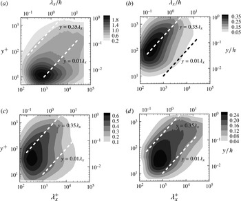
) appears to provide a better explanation of a number of features of the spectra of full simulations. Figure 14 shows one-dimensional streamwise spectra at
 $\mathit{Re}_{{\it\tau}}=2003$
(Hoyas & Jiménez Reference Hoyas and Jiménez2006) where the two curves
 $y=0.01{\it\lambda}_{x}$
and
 $y=0.35{\it\lambda}_{x}$
, given by eliminating
 ${\it\lambda}_{z}$
respectively from (5.1a,b
) and (5.1c,d
), are plotted together. The streamwise velocity spectra are very energetic along
 $y=0.01{\it\lambda}_{x}$
(figure 14
a) as the motions at (5.1a,b
) mainly carry the streamwise turbulent kinetic energy (figure 12
a). However, a considerable amount of energy along
 $y=0.35{\it\lambda}_{x}$
is also seen, as the motions at (5.1c,d
) also generate a non-negligible amount of streamwise turbulent kinetic energy (note that the spectral intensity of the streamwise velocity along
 $y=0.35{\it\lambda}_{x}$
is comparable with that of the wall-normal velocity in figure 12
b). On the other hand, the wall-normal velocity spectra are only energetic along
 $y=0.35{\it\lambda}_{x}$
(figure 14
b) as the streaky motions at (5.1a,b
) carry little wall-normal velocity (figure 12
b). Similar behaviour is seen in the spanwise velocity spectra, which are very energetic along
 $y\simeq 0.35{\it\lambda}_{x}$
. However, unlike the wall-normal velocity, they also contain a considerable amount of energy along
 $y=0.01{\it\lambda}_{x}$
(figure 14
c) because the motions at (5.1a,b
) also produce the spanwise velocity fluctuations to some extent (figure 12
c). The spectra of the Reynolds stress appear to be energetic in the region of
 $0.01{\it\lambda}_{x}\leqslant y\leqslant 0.35{\it\lambda}_{x}$
, as one might have expected from figure 12(d).
Premultiplied one-dimensional streamwise spectra of (a) streamwise, (b) wall-normal, (c) spanwise velocities and (d) Reynolds stress at
 $\mathit{Re}_{{\it\tau}}=2003$
(from Hoyas & Jiménez Reference Hoyas and Jiménez2006).

5.2.2.
 $k_{x}^{-1}$
spectra

The bimodal structure also appears to be associated with
 $k_{x}^{-1}$
behaviour in the one-dimensional streamwise spectra of streamwise velocity (Perry & Chong Reference Perry and Chong1982; Perry et al.
Reference Perry, Henbest and Chong1986; Perry & Marusic Reference Perry and Marusic1995; Nickels et al.
Reference Nickels, Marusic, Hafez and Chong2005). The
 $k_{x}^{-1}$
spectra are supposed to appear in the spectral region where scaling with the log-region length
 $y$
and the outer length
 $h$
is simultaneously valid (Perry et al.
Reference Perry, Henbest and Chong1986). According to Nickels et al. (Reference Nickels, Marusic, Hafez and Chong2005) and Hutchins & Marusic (Reference Hutchins and Marusic2007), this region emerges at considerably high Reynolds numbers (
 $\mathit{Re}_{{\it\tau}}>5000$
) and is bounded by
 $$\begin{eqnarray}y^{+}>100,\quad {\it\lambda}_{x}>15.7y\quad \text{and}\quad {\it\lambda}_{x}<0.3h,\end{eqnarray}$$
for turbulent boundary layers.
The bimodal structure given by (5.1a,b
) and (5.1c,d
) can be used to predict this region. The scaling (5.1c,d
) suggests that the spectral region scaling with the log-region length
 $y$
in the spectra would appear only along
 $y=0.35{\it\lambda}_{x}$
as there are no energetic motions contaminating the spectra at
 $y>0.35{\it\lambda}_{x}$
. Since the smallest spanwise length scale of the motions along (5.1c,d
) is
 ${\it\lambda}_{z}^{+}\simeq 100$
, the part of the spectra scaling in
 $y$
would appear at least for
 $y^{+}>70$
, resulting in the first condition. Second, figure 12(a) suggests that the streamwise velocity spectra given by (5.1c,d
) would be considerably weak for
 ${\it\lambda}_{x}>6{\it\lambda}_{z}$
at
 $y\simeq 0.5{\it\lambda}_{z}$
. Therefore, the region scaling with
 $y$
would roughly be bounded by
 $y<0.08{\it\lambda}_{x}~({\it\lambda}_{x}>12y)$
, yielding the second condition. Finally, the numerical experiment in § 3 suggests that the contribution made by the outer-scaling motions would be considerably weak for
 ${\it\lambda}_{x}<2h$
(figure 9
b), leading to the last condition. Taking these together, the spectral region, where the relevant length scale is not well defined between
 $y$
and
 $h$
, would be bounded by
 $$\begin{eqnarray}y^{+}>70,\quad {\it\lambda}_{x}>12y\quad \text{and}\quad {\it\lambda}_{x}<2h,\end{eqnarray}$$
and the only possible scaling in this region would be by being simultaneously valid with
 $y$
and
 $h$
, resulting in the
 $k_{x}^{-1}$
spectra. We note that the boundaries given by (5.5) are not very different from those in (5.4), except the last inequality in (5.5). However, the difference in the last inequality in (5.5) from that in (5.4) is also seen to be caused at least partially by the difference of the outer motions in a turbulent channel from those in a turbulent boundary layer, given the fact that the outer motions in boundary layers tend to be shorter and narrower than those in channels (Monty et al.
Reference Monty, Hutchins, NG, Marusic and Chong2009). Furthermore, the influence of the self-similar motions at (5.1a,b
) on this region would also be possible to some extent, indicating that the region of
 $k_{x}^{-1}$
spectra may be smaller than the one estimated by (5.5).
The argument based on (5.1a,b
) and (5.1c,d
) also suggests that
 $k_{x}^{-1}$
spectra would not appear in the wall-normal velocity spectra as they do not exhibit such a bimodal behaviour (figure 14
b) and the wall-normal component of the outer motions does not penetrate into the near-wall region (figure 9
d). However, the spanwise velocity spectra would have such a
 $k_{x}^{-1}$
dependence, given their bimodal behaviour (figure 14
c) and non-negligible contribution to the near-wall region (figure 9
f). The region of
 $k_{x}^{-1}$
dependence can be estimated through the same procedure: the spanwise velocity spectra associated with (5.1c,d
) are not energetic for
 ${\it\lambda}_{x}>10{\it\lambda}_{z}$
at
 $y\simeq 0.5{\it\lambda}_{z}$
(figure 12
c), and the spanwise velocity spectra of the outer motions are quite weak for
 ${\it\lambda}_{x}<h$
(figure 9
f). The boundaries of the
 $k_{x}^{-1}$
region in the spanwise velocity spectra would be estimated as
 $$\begin{eqnarray}y^{+}>70,\quad {\it\lambda}_{x}>20y\quad \text{and}\quad {\it\lambda}_{x}<h.\end{eqnarray}$$
Here, the boundaries given by (5.6) now yield a smaller region than those given by (5.5), indicating that the
 $k_{x}^{-1}$
behaviour in the spanwise velocity spectra may emerge at even higher Reynolds numbers than that in the streamwise ones. Finally, the Reynolds stress spectra would not be expected to have
 $k_{x}^{-1}$
spectra. We note that the last inequality in (5.5) and (5.6) implicitly contains the observation that the streamwise and spanwise components of the outer-scaling motion penetrate deep into the near-wall region (figure 9
b,d). However, such a behaviour would not be evident in the Reynolds stress spectra of the outer motions due to their very small wall-normal component in the near-wall region (figure 9
b,d). Therefore, it would be difficult to confidently build such an inequality for the Reynolds stress spectra. In this respect, it should be mentioned that the expectation of the emergence of the
 $k_{x}^{-1}$
behaviour only in the streamwise and spanwise velocity spectra has also been pointed out by previous studies (Kunkel & Marusic Reference Kunkel and Marusic2006; Nickels et al.
Reference Nickels, Marusic, Hafez, Hutchins and Chong2007), and the present discussion is consistent with these studies.
5.2.3. Two-dimensional spectra
The bimodal structure also provides some ideas on two-dimensional spectra in the logarithmic region. We multiply the left-hand terms in (5.1a,b ) and (5.1c,d ) respectively by the right-hand ones. Then, both (5.1a,b ) and (5.1c,d ) yield
 $$\begin{eqnarray}{\it\lambda}_{z}^{2}\simeq 1\sim 2{\it\lambda}_{x}y,\end{eqnarray}$$
the curve along which two-dimensional spectra of streamwise velocity have been found to be aligned (del Álamo et al.
Reference del Álamo, Jiménez, Zandonade and Moser2004). Given the nature of the streamwise velocity fluctuation affected by both (5.1a,b
) and (5.1c,d
), and the collective contribution of many self-similar energy-containing motions to a certain wall-normal location in the logarithmic region, it appears that the bimodal behaviour is associated with the alignment of the spectra along (5.7). We note that this feature has not been found in the spectra of wall-normal and spanwise velocities (del Álamo et al.
Reference del Álamo, Jiménez, Zandonade and Moser2004), which exhibit a single peak only along
 ${\it\lambda}_{x}\simeq {\it\lambda}_{z}$
close to the scaling in (5.1c,d
). While this behaviour in the spectra of wall-normal velocity is somehow expected given the single mode behaviour with (5.1c,d
), it is a little surprising to see this in the spanwise spectra. However, the amount of spanwise velocity fluctuation given by (5.1a,b
) is considerably smaller than that by (5.1c,d
) (figure 12
c), and this presumably explains why the two-dimensional spectra of spanwise velocity are rather similar to those of wall-normal velocity.
5.3. Inactive motions
The present numerical experiment has shown that the isolated energy-containing motions at each of the spanwise length scales carry a significant amount of Reynolds stress (figure 11). In particular, the amounts of turbulent kinetic energy and Reynolds stress solely by the outer motions (large-scale and very-large-scale motions) are only a little smaller even than those in the full simulation (figure 8), consistent with recent findings (Guala, Hommema & Adrian Reference Guala, Hommema and Adrian2006; Balakumar & Adrian Reference Balakumar and Adrian2007). It has often been mentioned that this energetic feature of the outer motions is contradictory to the attached-eddy theory, since Townsend (Reference Townsend1976) has often been believed to mention that large scales are ‘inactive’ in the sense that they do not carry Reynolds stress. However, this appears to be a misunderstanding stemming from an incorrect interpretation of his original discussion (p. 154 in Townsend Reference Townsend1976). In this section, we carefully follow the original discussion especially to understand what would be the ‘inactive’ motion in the attached-eddy theory.
We start by presenting the second paragraph on p. 154 in his book where the term ‘inactive’ is defined (Townsend Reference Townsend1976). The following are the first and second sentences of the paragraph:
‘It now appears that simple similarity of the motions is not possible with attached eddies, and, in particular, the stress–intensity ratio,
 $-\overline{uw}/\overline{q^{2}}$
, depends on some extent on position in the layer. The variation of the ratio does not invalidate the previous similarity analysis because the ‘non-similar’ logarithmic terms in the expression for
 $\overline{u^{2}}$
and
 $\overline{v^{2}}$
represent motions which are large-scale swirling in plane parallel to the wall and do not extract energy from the mean flow or affect the rate of energy transfer to smaller eddies for viscous dissipation.’
Here, in this original text,
 $q^{2}$
is turbulent kinetic energy, and
 $v$
and
 $w$
are the spanwise and wall-normal velocities, respectively. Given the logarithmic terms in (1.1a
) and (1.1b
), it is evident that the stress–intensity ratio is not constant along the wall-normal direction in the logarithmic region. However, since the attached-eddy theory is built upon the assumption of self-similarity of individual attached eddies, here he comments on the concern about the non-constant ratio. He justifies that the non-constant stress–intensity ratio would not be inconsistent with the self-similarity assumption, as the motions generating the logarithmic terms in (1.1a
) and (1.1b
) are not involved in extracting energy from the mean flow (see § 5.4 for further discussion). Although he explicitly mentioned that these motions are ‘large-scale’ swirling in plane parallel to the wall, it is not clear whether the ‘large-scale’ would mean the one often used to refer to ‘outer scale’. In the context, it rather appears to indicate the motions associated with the logarithmic terms, which, in fact, mathematically originate from the non-negligibly large streamwise and spanwise components of a single attached eddy in the region close to the wall (figure 2; see also the derivation given by Perry & Chong Reference Perry and Chong1982). Therefore, it would be more appropriate to view the ‘large-scale swirling’ as a motion generating the streamwise and spanwise components of a single attached eddy in the region close to the wall.
If the ‘large-scale swirling’ is interpreted in this way, the next sentence becomes more clear:
‘Swirling motions contribute little to the Reynolds stress, and their effect on that part of the layer between the point of observation and the wall is one of slow random variation of ‘mean velocity’ which cause corresponding variation of wall stress.’
Since the impermeability condition does not allow the wall-normal component of single attached eddy to reach the region close to the wall, there is no way for the swirling motions to generate the Reynolds stress. What is very interesting here is that he was also pointing out that the swirling motions would affect wall-shear stress, the feature confirmed only recently by our previous numerical experiment where the motions at the log-layer length scale were shown to involve generation of turbulent skin friction (Hwang Reference Hwang2013). However, it is not clear whether he meant that the swirling motions would also contribute to the ‘mean’ of turbulent skin friction, given the term, ‘random’.
In the following sentences, the term ‘inactive’ is defined:
‘It is possible and useful to regard the ‘swirl’ component of the local motion as an ‘inactive’ component which may be ignored in any discussion of the local flow, for example when using similarly assumptions to interpret the turbulent equation as an equation for the Reynolds stress. On the other hand, the inactive flow at one level is an essential part of active flow at other higher levels and ….’
Here, he more precisely mentions that the swirling motions, which do not carry Reynolds stress, would be a ‘component’ of some local motion rather than a body of the entire motion, which may be interpreted as the entire attached eddy at the given location. However, he points out that the inactive component could also be an essential part of the entire attached eddy which carries the Reynolds stress at a different location (i.e. active flow at other higher levels). Given this interpretation, it would be reasonable to view the ‘inactive’ component as the part of individual attached eddy which contributes to the region close to the wall through its streamwise and spanwise components without generating the Reynolds stress.
Adopting this interpretation, it appears that the ‘inactive component’ of the attached eddies would be associated with each of the long streaky motions at (5.1a,b
). As discussed, the streaky motions tend to penetrate deep into the region close to the wall, yielding a non-negligible amount of streamwise and spanwise velocity fluctuations in this region (figure 12
a,c). Each of the streaky motions below
 $y\simeq 0.05L_{z}$
shows very little Reynolds stress (figure 12
d), indicating that it would be regarded as the ‘inactive component’ of a single attached eddy. We note that the streaky motion itself is an essential part of the given single attached eddy (see also § 5.4), but it generates the Reynolds stress at
 $y\geqslant 0.1L_{z}$
(figure 12
d). In view of these observations, the computed attached eddies are consistent with those given in the original theory of Townsend (Reference Townsend1976).
5.4. Linear theories and the beyond
A number of recent theoretical studies, using a linearised Navier–Stokes equation with an eddy viscosity, have shown that long streaky motions can be significantly amplified at all length scales varying from the inner to outer units (del Álamo & Jiménez Reference del Álamo and Jiménez2006; Cossu et al. Reference Cossu, Pujals and Depardon2009; Hwang & Cossu Reference Hwang and Cossu2010a ,Reference Hwang and Cossu b ; Pujals et al. Reference Pujals, García-Villalba, Cossu and Depardon2010; Willis et al. Reference Willis, Hwang and Cossu2010). In particular, the computed streaks contributing to the logarithmic region in these studies have been found to be self-similar with the spanwise length (Hwang & Cossu Reference Hwang and Cossu2010b ). This theoretical finding is consistent with the present numerical experiment where such self-similar streaky motions with the spanwise length emerge through (5.1a,b ). Therefore, the present numerical experiment also suggests that the streaky motions are likely to be a consequence of the lift-up effect, i.e. tilting of streamwise vortices by mean shear:
 $$\begin{eqnarray}\frac{\text{D}{\it\omega}_{y}}{\text{D}t}\sim \frac{\text{d}U}{\text{d}y}{\it\omega}_{x},\end{eqnarray}$$
where
 $\text{D}/\text{D}t$
is the material time derivative, and
 ${\it\omega}_{x}$
and
 ${\it\omega}_{y}$
are the streamwise and wall-normal vorticity, respectively. We note that (5.8) also exactly represents the off-diagonal term in the Orr–Sommerfeld–Squire operator (linearised Navier–Stokes operator), and is the main contributor to the strong non-normality of the operator (e.g. Schmid & Henningson Reference Schmid and Henningson2001). Also, (5.8) indicates that the streaky motions are a ‘consequence’ of energy transfer from the mean shear by streamwise vortices: i.e. the streaky motions themselves do not take energy from the mean shear. This is consistent with Townsend (Reference Townsend1976) who mentioned that the inactive component does not take energy from the mean shear (see § 5.3).
Nevertheless, one should also note that the streaky motions in the present numerical experiment are not fully consistent with the most amplified ones in the previous linear theories. First, the self-sustaining attached eddies in the present study contain considerably strong vortical structures scaling with (5.1c,d ), while the most amplified flow structures in the linear theories contain very weak vortical structures. Second, although the streaky motions in the present study are generally long, their streamwise length is certainly finite as in (5.1a,b ). However, the most amplified streaky motions in the linear theories are infinitely long (Hwang & Cossu Reference Hwang and Cossu2010b ; Pujals et al. Reference Pujals, García-Villalba, Cossu and Depardon2010). Finally, the streaky motions in the present study are certainly advected downstream whereas the most amplified ones in the linear theories are stationary (del Álamo & Jiménez Reference del Álamo and Jiménez2006; Cossu et al. Reference Cossu, Pujals and Depardon2009; Hwang & Cossu Reference Hwang and Cossu2010a ; Pujals et al. Reference Pujals, García-Villalba, Cossu and Depardon2010).
It appears that all of these inconsistent features would be because the linearised Navier–Stokes operator does not contain well-defined physical mechanisms for generation of the short and tall vortical structures scaling with (5.1c,d
). In general, the Orr–Sommerfeld–Squire system operator does not have any mathematical structure to drive such vortical structures which contain an intense wall-normal velocity fluctuation except through the Orr–Sommerfeld equation itself (see also below): i.e. the Squire equation, which describes the evolution of the streaks, is passive to the Orr–Sommerfeld equation. Indeed, in the near-wall region, such vortical structures (i.e. quasi-streamwise vortices) have been found to be a consequence of instability and/or transient growth of the amplified streaks and the following nonlinear processes (Hamilton et al.
Reference Hamilton, Kim and Waleffe1995; Schoppa & Hussain Reference Schoppa and Hussain2002). Here, it should be pointed out that the streak instability (or transient growth) mechanism characterises the streamwise length scale of the near-wall motions. The streamwise wavelength of the most unstable mode for the amplified near-wall streaks is
 ${\it\lambda}_{x}^{+}\simeq 300$
, close to the streamwise size of the quasi-streamwise vortices (Schoppa & Hussain Reference Schoppa and Hussain2002). The streamwise wavelength of the instability is bounded to
 ${\it\lambda}_{x}^{+}\simeq O(1000)$
, indicating that streaky motions longer than this would not appear, as also confirmed by Jiménez et al. (Reference Jiménez, del Álamo and Flores2004). It appears that this mechanism is also applicable to the outer motions. Indeed, Park, Hwang & Cossu (Reference Park, Hwang and Cossu2011) have recently shown that the most unstable mode of the streak (i.e. VLSM) instability in the outer region appears at
 ${\it\lambda}_{x}\simeq 3h\sim 5h$
, comparable with the streamwise length of the outer vortical structures (LSMs). The streak instability wavelength is bounded by
 ${\it\lambda}_{x}\simeq 10h\sim 20h$
, consistent with the streamwise length scale of the VLSMs (Park et al.
Reference Park, Hwang and Cossu2011). Finally, it should be pointed out that the streak instability also appears to give the ‘speed’ of the streaky motions: the most unstable wave contains non-zero phase speed, which is often given by the critical layer of the corresponding ‘two-dimensional streaky’ base flow (Andersson et al.
Reference Andersson, Brandt, Bottaro and Henningson2001; Schoppa & Hussain Reference Schoppa and Hussain2002; Park et al.
Reference Park, Hwang and Cossu2011). This implies that the vortical structures feeding the streaky motions through (5.8) would have a certain speed, eventually resulting in the speed of the streaky motions as in the present study.
The process beyond the streak instability, which would play a significant role in amplifying the streamwise vortices, has been much less studied due to their strong nonlinear nature. For the near-wall motions in turbulent channel flow, Schoppa & Hussain (Reference Schoppa and Hussain2002) have proposed that the nonlinear process is associated with vortex stretching caused by the streamwise wavy mean shear due to the streaky instability and/or transient growth. On the other hand, for the motions in the logarithmic and the outer regions, Jiménez (Reference Jiménez2013b ) has proposed that the Orr mechanism plays a certain role at this nonlinear stage in conjunction with the streaky instability, although it is also inherent in the linearised Navier–Stokes operator (i.e. Orr–Sommerfeld operator). Apart from this cyclic-dynamics framework, it is finally worth mentioning the recent work by Sharma & Mckeon (Reference Sharma and Mckeon2013), who proposed the emergence of a ‘packet-like’ vortical structure by building a triadic interaction among the leading resolvent modes of the linearised Navier–Stokes operator. Despite such recent progress, our understanding beyond the linear theories is still very limited, and this remains an important subject of future study.
6. Concluding remarks
The main findings are summarised as follows:
-
(a) A numerical experiment, which isolates energy-containing motions at a given spanwise length scale
${\it\lambda}_{z}={\it\lambda}_{z,0}$
in
$100{\it\delta}_{{\it\nu}}<{\it\lambda}_{z,0}\leqslant 1.5h$
, has been performed. The motions at
${\it\lambda}_{z}<{\it\lambda}_{z,0}$
are removed by applying the explicit filtering in Hwang (Reference Hwang2013), while those at
${\it\lambda}_{z}>{\it\lambda}_{z,0}$
are damped out using the over-damped LES in Hwang & Cossu (Reference Hwang and Cossu2010c
). The numerical technique successfully builds a simulation which simulates only the energy-containing motions at the prescribed spanwise length scale, confirming the self-sustaining nature of the motions in the logarithmic and the wake outer regions (Hwang & Cossu Reference Hwang and Cossu2010c
, Reference Hwang and Cossu2011). -
(b) The numerical experiment has revealed that the statistical structure of each of the self-sustaining energy-containing motions is self-similar with the spanwise length scale proportional to the distance of the wall. The self-similar statistical structure has also been found to be consistent with that of the attached eddies at a given length scale in Townsend (Reference Townsend1976) and Perry & Chong (Reference Perry and Chong1982), suggesting that the self-sustaining energy-containing motions at a given spanwise length scale are the attached eddies.
-
(c) The numerical experiment has suggested that the there exist two distinct motions which could be interpreted as two dynamically interconnected elements of a single attached eddy: one is a long streaky motion carrying intense streamwise turbulent kinetic energy and some spanwise energy, and the other is a short and tall vortical structure containing all the velocity components. The former is self-similar through the scaling (5.1a,b ) while the latter is self-similar through the scaling (5.1c,d ). The self-similarity established with (5.1a,b ) and (5.1c,d ) suggests that a near-wall coherent motion, composed of a streak and quasi-streamwise vortices aligned to that, would be the smallest attached eddy, whereas an outer coherent motion, in the form of a VLSM and LSMs aligned to that, would be the largest attached eddy.
-
(d) A further discussion has revealed that the bimodal behaviour of the single attached eddy given by (5.1a,b ) and (5.1c,d ) provides a plausible explanation for a number of important features in full spectra including
$k_{x}^{-1}$
behaviour, and is also consistent with several recent theoretical findings.




Predicting turbulent statistics without performing laboratory experiment or DNS has been a long-standing interest for engineering applications. In particular, in a series of works refined by Perry and coworkers over a number of years (Perry & Chong Reference Perry and Chong1982; Perry et al.
Reference Perry, Henbest and Chong1986; Perry, Lim & Chong Reference Perry, Lim and Chong1990; Perry, Li & Marusic Reference Perry, Li and Marusic1991a
; Perry, Marusic & Li Reference Perry, Marusic and Li1991b
; Marusic & Perry Reference Marusic and Perry1995; Perry & Marusic Reference Perry and Marusic1995), the attached-eddy hypothesis was the backbone for the construction of turbulent statistics by enabling them to prescribe the eddy population density and the relevant velocity scale in a self-consistent manner. In these works, the statistical structure of the attached eddies at a given scale was required to complete the entire analysis (Perry et al.
Reference Perry, Marusic and Li1991b
; Perry & Marusic Reference Perry and Marusic1995), but this part had to be modelled with a simplified eddy (e.g.
 ${\it\Lambda}$
or hairpin vortices) due to the lack of data. While the present study directly supports the early theoretical works, it could also be used to improve them. In particular, the statistical structure of the attached eddies at a given length scale would become a new input for the analysis instead of the specific eddy structure modelled, and this remains important work to be done in the future.
Finally, it should be emphasised that the self-similar nature of the self-sustaining energy-containing motions, each of which is composed of streaks and vortices, also has a very important implication for a number of previous findings on the ‘exact coherent structures’: i.e. the exact solutions of the Navier–Stokes equation given in the form of unstable equilibria, travelling waves, and periodic orbits (e.g. Nagata Reference Nagata1990; Waleffe Reference Waleffe1998, Reference Waleffe2001, Reference Waleffe2003; Faisst & Eckhardt Reference Faisst and Eckhardt2003; Wedin & Kerswell Reference Wedin and Kerswell2004; Jiménez et al. Reference Jiménez, Kawahara, Simens, Nagata and Shiba2005; Gibson, Halcrow & Cvitanovic Reference Gibson, Halcrow and Cvitanovic2008; Hall & Sherwin Reference Hall and Sherwin2010). At low Reynolds number where the inner and outer length scales are almost identical, these solutions have been understood to guide the near-wall self-sustaining process by forming a skeleton of the turbulent solution trajectory in phase space (e.g. Gibson et al. Reference Gibson, Halcrow and Cvitanovic2008), significantly advancing our understanding on bypass transition and low-Reynolds-number turbulence.
Nevertheless, extending such approaches to high-Reynolds-number turbulence has often been thought a daunting task because a huge number of exact solutions emerge with the increase of the Reynolds number, yielding a difficulty in identifying which solution would be the best representation of a given coherent structure. Performing a numerical experiment, such as the one in the present study, is important in this regard, as it provides a way to reduce the dimension of the high-Reynolds-number turbulence without significantly distorting important physical features of the given coherent structure. More importantly, the present numerical experiment has shown that the individual attached eddies would be given almost in the same form as the near-wall coherent motions: i.e. self-similar streaky motions and vortical structures. This suggests that the attached eddies may also be a physical-space reflection of these mathematical entities, the number of which also significantly increases with the Reynolds number. In this respect, it is important to emphasise that the attached-eddy hypothesis would act as a theoretical bridge between the ‘real’ and ‘exact’ coherent structures, as it would show the physical implications of the exact solutions at high Reynolds numbers. Constructing such a bridge would significantly advance the theoretical description of wall-bounded flows in a wide range of Reynolds numbers, and this is a subject of our current investigation.
Appendix A. Comparison of the reference LES with DNS
Here, the spectra of
 $F950$
(figure 9
a,c,e,g) are compared with those of DNS (del Álamo et al.
Reference del Álamo, Jiménez, Zandonade and Moser2004) shown in figure 15. Overall, the peak locations in the spectra of
 $F950$
appear in good agreement with those of DNS, indicating that the energy-containing motions in
 $F950$
are reasonably well resolved. In particular, due to the long streamwise domain (
 $L_{x}=12{\rm\pi}$
), the streamwise velocity spectra of
 $F950$
exhibit a tendency to be closed at
 ${\it\lambda}_{x}>20h$
. On the contrary, the spectra of the DNS are not completely closed, indicating that the streamwise domain of DNS (
 $L_{x}=8{\rm\pi}$
) might have influenced the spectra for
 ${\it\lambda}_{x}>10h$
. However, since
 $F950$
is an LES, its small-scale motions appear to be clearly not well resolved especially for
 ${\it\lambda}_{x}^{+}<477~({\it\lambda}_{x}<0.5h)$
and
 $y^{+}>100~(y>0.1h)$
. In this region, all the spectra of
 $F950$
show more energy than those of DNS, indicating that
 $F950$
probably contains some numerical error at the small scales associated with the energy cascade in the logarithmic and the wake outer regions.
Premultiplied one-dimensional streamwise spectra of (a) streamwise, (b) wall-normal, (c) spanwise velocities and (d) Reynolds stress at
 $\mathit{Re}_{{\it\tau}}=934$
(del Álamo et al.
Reference del Álamo, Jiménez, Zandonade and Moser2004).

Appendix B. Statistics on increasing
$C_{s}$
with a restricted spanwise computational domain

Here, we present the change of the wall-normal profiles of the first- and second-order statistics in a narrow spanwise domain with the filtering (2.2) on increasing
 $C_{s}$
, and this is reported in figure 16. As in figure 8, the mean-velocity profile exhibits a non-trivial change on increasing
 $C_{s}$
(figure 16
a). Given the fact that the simulations for
 $C_{s}>0.05$
do not contain a significant number of energy-containing motions, this would not be very surprising. As
 $C_{s}$
is increased, the turbulence intensities also exhibit a similar behaviour to the case with the very large domain (i.e. figure 8): the intensities of all the velocity components are gradually quenched from the near wall on increasing
 $C_{s}$
, except the streamwise velocity fluctuation which reveals intensification of the peak as in the case with the full domain (figure 16
b–d). However, in this case, the intensities for
 $y>0.5L_{z}$
are also seen to be affected a little by the increase of
 $C_{s}$
(
 $C_{s}\gtrsim 0.2$
in this case). We note that this part of the velocity fluctuations is not self-similar (figure 11) and that they appear to be induced by the self-similar part for
 $y\lesssim 0.5L_{z}$
, given their streamwise length scale shown in the streamwise spectra (figure 12). This nature of the fluctuations at
 $y>0.5L_{z}$
is different from the outer part of the fluctuations in the full simulation which has an independent generation mechanism (see § 3), and this probably explains why the intensities for
 $y>0.5L_{z}$
with narrow spanwise domain are a little affected by the increase of
 $C_{s}$
.
Statistics with the increase of
 $C_{s}$
for
 $L1800b$
simulation: (a) mean-velocity profile (
 $U_{c}^{+}$
the centreline velocity); (b) streamwise and spanwise turbulent intensities; (c) wall-normal turbulent intensity; (d) Reynolds stress. Here, ——,
 $C_{s}=0.05$
; - - - -,
 $C_{s}=0.10$
; – - – - –,
 $C_{s}=0.20$
; –
 $\cdot \cdot$
–
 $\cdot \cdot$
–,
 $C_{s}=0.30~(L1800b)$
.