1. Introduction
When a disturbed interface separating two fluids with different densities is accelerated by a shock wave, the Richtmyer–Meshkov (RM) instability occurs (Richtmyer Reference Richtmyer1960; Meshkov Reference Meshkov1969). The initial perturbations generally develop linearly at early times, and then the amplitude growth reaches a nonlinear state with characteristic bubbles and spikes, and eventually a turbulent mixing zone between the two fluids appears. The RM instability can be found in both natural and engineering applications, such as the formation of structures of supernova remnants (Kane, Drake & Remington Reference Kane, Drake and Remington1999), supersonic combustion ramjets (Yang, Kubota & Zukoski Reference Yang, Kubota and Zukoski1993), inertial confinement fusion (Lindl et al. Reference Lindl, Landen, Edwards, Moses and Team2014) and some others. In these applications, the interface would experience multiple shocks and reshocks because of boundary walls or special geometries, which have motivated the study of RM instability upon reshock for understanding the underlying mechanisms of different phenomena (Zhou Reference Zhou2017a,Reference Zhoub).
In early experiments of RM instability under reshock, initial interfaces with small-scale arbitrary perturbations were considered. Discontinuous interfaces were formed by a nitrocellulose membrane (Brouillette & Sturtevant Reference Brouillette and Sturtevant1989, Reference Brouillette and Sturtevant1993) and continuous interfaces were generated by pulling off a sliding plate between two gases (Brouillette & Sturtevant Reference Brouillette and Sturtevant1994). The results indicated that the width growths after reshock were dramatically increased compared with those before reshock. Leinov et al. (Reference Leinov, Malamud, Elbaz, Levin, Ben-Dor, Shvarts and Sadot2009) used the nitrocellulose membrane to create three-dimensional (3-D) multi-mode perturbations, and found that the perturbation growths after reshock were independent of the interface shapes at the time of reshock arrival. To eliminate the potential influence of the fragment pieces on the evolution, the membraneless technique was adopted, and two distinct interfaces with 3-D random perturbations were generated by vertically oscillating the gas column within a vertical shock tube (Jacobs, Krivets & Tsiklashvili Reference Jacobs, Krivets and Tsiklashvili2013). The experiments showed a smaller mixing width growth rate after reshock with a similar insensitivity of growths to the interface shape at the time of reshock arrival in comparison with the findings in Leinov et al. (Reference Leinov, Malamud, Elbaz, Levin, Ben-Dor, Shvarts and Sadot2009). In these studies, due to the initial arbitrary multi-mode perturbations, the mixing layers were fully developed before reshock; thus, a weak dependence of perturbation growths on the initial interface shapes was found.
Later, some single-scale interfaces such as gas curtains (Balakumar et al. Reference Balakumar, Orlicz, Tomkins and Prestridge2008, Reference Balakumar, Orlicz, Ristorcelli, Balasubramanian, Prestridge and Tomkins2012) and inclined interfaces (McFarland et al. Reference McFarland, Reilly, Creel, McDonald, Finn and Ranjan2014; Reilly et al. Reference Reilly, McFarland, Mohaghar and Ranjan2015) were formed through the membraneless technique. The arrival time of the reshock impacting the distorted interface was controlled in the nonlinear stage where the interface was heavily diffused, making the mixing layer chaotic rapidly. The turbulence statistics results were found to be sensitive to initial conditions (Balasubramanian et al. Reference Balasubramanian, Orlicz, Prestridge and Balakumar2012). However, the perturbation growth was independent of the distorted interface shapes at the time of reshock arrival (Mohaghar et al. Reference Mohaghar, Carter, Musci, Reilly, McFarland and Ranjan2017, Reference Mohaghar, Carter, Pathikonda and Ranjan2019), similar to the findings of Leinov et al. (Reference Leinov, Malamud, Elbaz, Levin, Ben-Dor, Shvarts and Sadot2009) and Jacobs et al. (Reference Jacobs, Krivets and Tsiklashvili2013). It can be seen that these experiments mainly focus on the turbulent mixing stage of RM instability, possibly due to the limitation of initial interface generation methods. However, if the distorted interface at the time of reshock arrival is still approximately single-scale (e.g. the interface still develops in the weakly nonlinear stage), ordered flow fields would be maintained during the early development of RM instability upon reshock, different from the evolution of chaotic mixing layers. Therefore, performing related studies would be helpful for understanding the initial condition dependence of perturbation growths in shock-accelerated flows upon reshock.
The single-mode shape is the basis of complex geometry, one of the most commonly used subjects in previous studies of RM instability (Zhou Reference Zhou2017a,Reference Zhoub). Recently, two-dimensional (2-D) well-defined single-mode and quasi-single-mode interfaces have been successfully generated by a soap-film technique (Liu et al. Reference Liu, Liang, Ding, Liu and Luo2018; Liang et al. Reference Liang, Zhai, Ding and Luo2019; Guo et al. Reference Guo, Zhai, Ding, Si and Luo2020). From the spectrum analysis, the quasi-single-mode interfaces have a fundamental mode and a number of high-order modes, in which the fundamental mode has the largest absolute value of coefficients that is smaller or larger than unity (Liang et al. Reference Liang, Zhai, Ding and Luo2019). In experiments, clear interface morphologies that are hardly influenced by either fragment pieces or the presence of a diffuse interface layer were captured. In these singly shocked experiments, the fundamental mode of quasi-single-mode interfaces was found to dominate the perturbation growth with similar evolutions of the single-mode interface. In reshock experiments with initial single-mode (Collins & Jacobs Reference Collins and Jacobs2002; Weber et al. Reference Weber, Haehn, Oakley, Anderson and Bonazza2012) or quasi-single-mode (Hahn et al. Reference Hahn, Drikakis, Youngs and Williams2011; Mohaghar et al. Reference Mohaghar, Carter, Musci, Reilly, McFarland and Ranjan2017, Reference Mohaghar, Carter, Pathikonda and Ranjan2019) interfaces, light/heavy configurations (the incident shock propagates from the light fluid to the heavy fluid) are often considered, while studies with heavy/light configurations (the incident shock propagates from the heavy fluid to the light fluid) seem to be rare (Hahn et al. Reference Hahn, Drikakis, Youngs and Williams2011). More importantly, most classical theories proposed for singly shocked cases (Richtmyer Reference Richtmyer1960; Sadot et al. Reference Sadot, Erez, Alon, Oron, Levin, Erez, Ben-Dor and Shvarts1998; Dimonte & Ramaprabhu Reference Dimonte and Ramaprabhu2010; Zhang & Guo Reference Zhang and Guo2016) or reshock cases (Mikaelian Reference Mikaelian1989, Reference Mikaelian2011, Reference Mikaelian2015; Charakhch'yan Reference Charakhch'yan2000) have been frequently tested in the experiments with an initial light/heavy interface (Vetter & Sturtevant Reference Vetter and Sturtevant1995; Leinov et al. Reference Leinov, Malamud, Elbaz, Levin, Ben-Dor, Shvarts and Sadot2009; Morgan et al. Reference Morgan, Aure, Stockero, Greenough, Cabot, Likhachev and Jacobs2012; Weber et al. Reference Weber, Haehn, Oakley, Rothamer and Bonazza2014; Mansoor et al. Reference Mansoor, Dalton, Martinez, Desjardins, Charonko and Prestridge2020). However, the RM instability with or without reshock of an initial heavy/light interface (Brouillette & Sturtevant Reference Brouillette and Sturtevant1989, Reference Brouillette and Sturtevant1993) is far different from that of the light/heavy one. Therefore, it is necessary to further study the RM instability for the heavy/light case especially upon reshock and explore the applicable physical models in understanding the corresponding growth mechanisms.
In this work, we aim to perform experimental studies on the RM instability of heavy/light interfaces with initial single-mode and quasi-single-mode shapes upon reshock. Three types of initially perturbed  ${\rm SF}_6/{\rm air}$ interfaces are generated through the soap-film technique. By choosing a reflection distance that can ensure that the first reshock arrives at the distorted interface developing in the weakly nonlinear stage, the evolution of approximately single-scale interfaces is achieved. Clear interface morphologies are captured by the high-speed schlieren photography, and the structural evolutions of interfaces with different initial shapes before and after reshock are compared. The high-fidelity images allow us to extract the interface contour and carry out the Fourier analysis to obtain the mode information. From the mode analysis, the interface evolutions for different interface shapes before and after reshock are obtained. Based on the reliable experimental results, the applicability of the existing theoretical models is tested for the heavy/light case, and the application scope of the model is extended to the phase after reshock.
2. Experimental methods
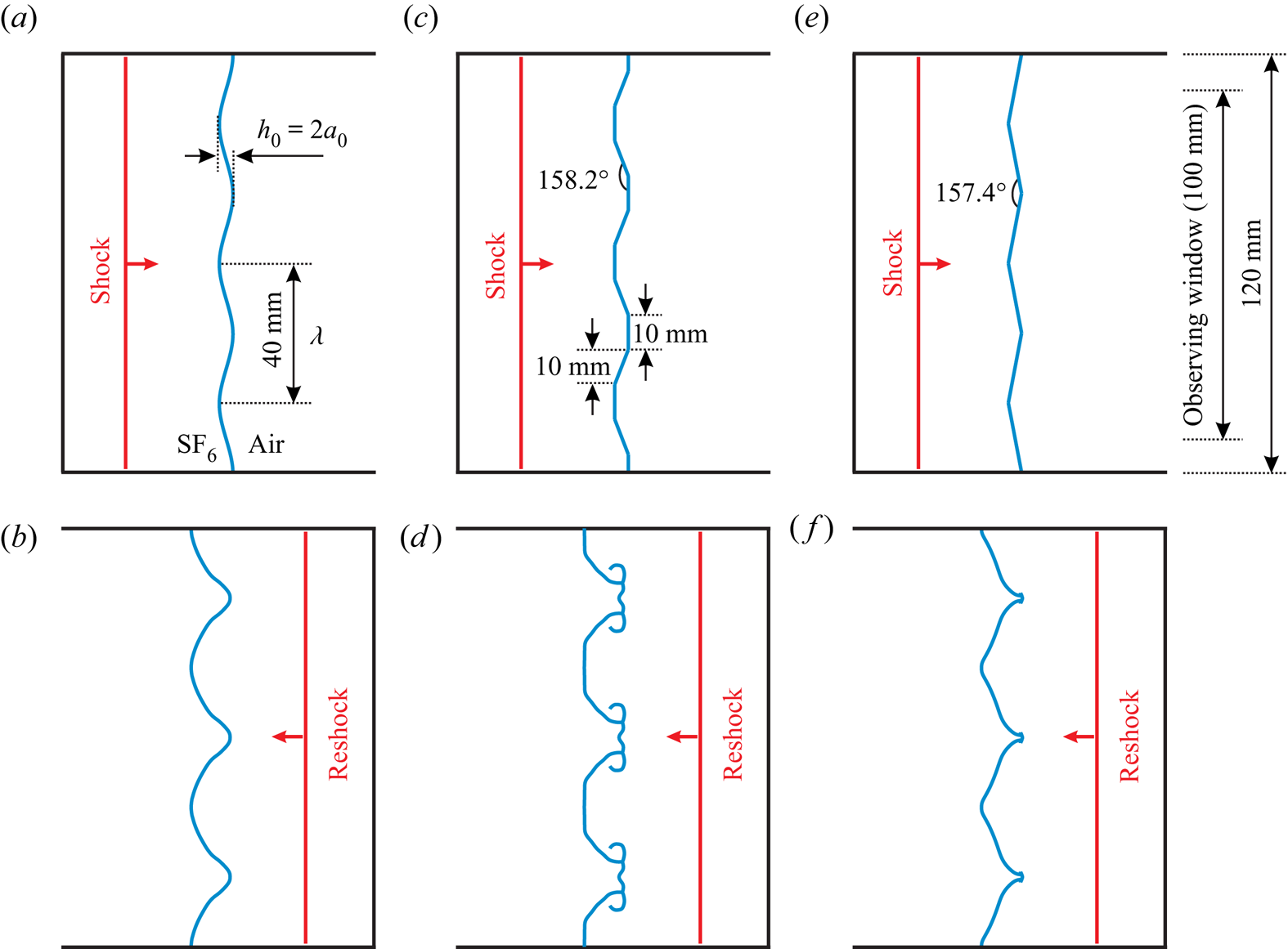
The experiments are conducted in a horizontal shock-tube facility manufactured in our group (Liu et al. Reference Liu, Liang, Ding, Liu and Luo2018; Liang et al. Reference Liang, Zhai, Ding and Luo2019). Different initial interfaces can be formed in the test section. In this work, the single-mode (SM) interface and two typical quasi-single-mode interfaces with trapezoid (TR) and sawtooth (ST) shapes are considered, as shown in figure 1. The TR and ST interfaces are actually multi-mode interfaces, but have evident shape features of the SM interface: the amplitude of the first mode is much larger than that of high-order modes. The SM shape can be described by a cosine function, and the Fourier expansions of TR and ST interfaces can be expressed as follows:
 $$\begin{gather} y_{TR}=a_{0}[{-}1.146\cos(kx)+0.127\cos(3kx)+0.046\cos(5kx)-\cdots], \end{gather}$$
 $$\begin{gather}y_{ST}=a_{0}[{-}0.811\cos(kx)-0.090\cos(3kx)-0.032\cos(5kx)-\cdots], \end{gather}$$
with  $a_0$ the initial amplitude and
 $k$ the wavenumber. It can be easily seen that the first mode of the interface is dominant (i.e. defined as the fundamental mode). One can further find that, for the TR interface, the signs of each mode are minus and plus alternately, while for the ST interface, the signs of each mode are the same.
Schematics of interface morphologies for the SM (a,b), TR (c,d) and ST (e, f) interfaces before the arrival of the incident shock (a,c,e) and the first reshock (b,d, f). Here  $h_0$,
 $a_0$ and
 $\lambda$ denote the initial width, amplitude and wavelength of the interface, respectively.

In the experiments, the initial amplitude ( $a_0$) and wavelength (
 $\lambda$) of the SM, TR and ST interfaces are fixed to be 2 and 40 mm, respectively, satisfying the small-perturbation hypothesis (i.e.
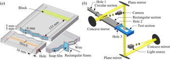
 $a_0/\lambda = 0.05$). Every initial interface is periodically formed, which eliminates the effect of non-periodic portions on the interface evolution (Luo et al. Reference Luo, Liang, Si and Zhai2019). Taking the ST interface as an example, the interface formation device used in each experimental run is shown in figure 2(a). An acrylic block as the endwall is glued by chloroform and silicone rubber to the right side of the interface formation device to form the reshock. For the SM interface, the adjacent boundaries of the upper and lower plates are carefully engraved to be of a sinusoidal shape to restrict the soap film to the designed form (Liu et al. Reference Liu, Liang, Ding, Liu and Luo2018). For the TR and ST interfaces, thin wires (0.128 mm in diameter) are introduced at each corner to avoid pressure singularity (Isenberg Reference Isenberg1992; Guo et al. Reference Guo, Zhai, Si and Luo2019). Before generating the interface, the edges of the interface device are wetted by a mixed solution (made of 60 % clean water, 20 % concentrated liquid soap and 20 % glycerine by volume) prepared in advance. Then, as shown in figure 2(a), a rectangular frame, the edges of which have been dipped into a proper amount of soap solution, is pulled along the edges of the interface device. Eventually, a soap-film interface with the designed shape is generated.
Schematics of the interface formation device (a) and the high-speed schlieren system (b).

In order to form the  ${\rm SF}_6/{\rm air}$ gaseous interface in each experimental run, a strict procedure is needed. After the interface formation device with the prepared soap-film interface is carefully inserted into the test section,
 ${\rm SF}_6$ is inflated into the rectangular section through hole 2, as shown in figure 2(b). Then,
 ${\rm SF}_6$ diffuses into the test section and is discharged from hole 3 at both sides of the test section. For all experimental cases, the inflation rate and time are kept the same. As a result, the difference of volume fraction of
 ${\rm SF}_6$ (air) at the left (right) side of the interface in each run is negligible. In our work, at least three successful experimental runs are performed for each case to ensure the repeatability of the experiments. The incident (
 $217.4 \pm 1.0\ {\rm m}\ {\rm s}^{-1}$) and transmitted (
 $413.0 \pm 1.0\ {\rm m}\ {\rm s}^{-1}$) shock velocities for each case are nearly identical, verifying that the initial experimental parameters for each case are almost the same. The detailed initial parameters are listed in table 1, in which
 $A = (\rho _2-\rho _1)/(\rho _2+\rho _1)$ is the Atwood number, with
 $\rho _2$ and
 $\rho _1$ being the densities of gases at the right-hand and left-hand sides of the interface, respectively. The post-shock flow field is recorded by a high-speed schlieren system, as shown in figure 2(b). The frame rate of the high-speed video camera (FASTCAM SA5, Photron Ltd) is 50 000 frames per second, and the exposure time is
 $1\ \mathrm {\mu }{\rm s}$. The pixel resolution is about 0.43 mm pixel
 $^{-1}$. The ambient pressure and temperature are 101.3 kPa and
 $300 \pm 1.5$ K, respectively.
Experimental parameters:  $M_i$ is the Mach number of the incident shock wave; VFL and VFR are the volume fractions of
 ${\rm SF}_6$ at the left and right side of the interface, respectively;
 $A$,
 $A^{+}$ and
 $A^{+}_r$ are the pre-shock, post-shock and post-reshock Atwood numbers; and
 $\Delta V_1$,
 $\Delta V_{1r}$ and
 $\Delta V_{2r}$ are the jump velocities for a flat interface induced by the incident shock, the first reshock and the second reshock, respectively. The unit of velocities is
 ${\rm m}\ {\rm s}^{-1}$.

It must be mentioned that the interface evolution induced by the reshock would be heavily dependent on the shape of the distorted interfaces at the time of first reshock arrival, which makes the problem very complex. In this work, the reflection distance defined as the distance between the initial interface centre and the endwall is specifically set, ensuring that the interface shape maintains a single-value function for a certain time before reshock, and thus the effects of reshock on mode evolution can be investigated based on Fourier analysis. For this purpose, a typical reflection distance is selected as 155 mm (slightly larger or smaller values would lead to similar phenomena). In this situation, the perturbation amplitude growth can be located in the weakly nonlinear stage at the time of first reshock arrival, where the vortices on the interface are not evident and the interface is approximately single-scale.
3. Experimental results and analysis
3.1. Interface morphology and flow features
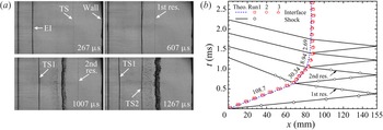
The complete evolution of the interaction between an unperturbed interface with the incident planar shock and the reshocks is examined first. The formation of a flat soap-film interface located at a position with a reflection distance of 155 mm is given following the same schedule as described above. The motion trajectories of the shock waves and the initial flat  ${\rm SF}_6/{\rm air}$ interface accelerated by the incident shock wave with
 $M_i = 1.317$ are presented in figure 3. Interface displacements in three different experimental runs are plotted, and a good agreement with theories can be observed, verifying the good repeatability of experiments. After the incident shock wave impinges the unperturbed interface, it obtains a jump velocity (
 $108.7\ {\rm m}\ {\rm s}^{-1}$) and moves uniformly. Then, multiple reshocks moving from the endwall impact the distorted interface, making it decelerate gradually. The first and the second reshocks can reduce the interface velocity from
 $108.7\ {\rm m} {\rm s}^{-1}$ to
 $30.34\ {\rm m}\ {\rm s}^{-1}$ and to
 $8.94\ {\rm m}\ {\rm s}^{-1}$ quickly. This indicates that the first two reshocks have the most significant effects on the interface evolution, and the later reshocks become weak.
Evolution of the undisturbed  ${\rm SF}_6/{\rm air}$ interface (a), and wave diagram for the interaction of an
 $M_i = 1.317$ shock wave with the undisturbed interface (b). Here EI is the evolving interface; 1st res. and 2nd res. are the reshocks reflected from the endwall for the first and second time; and TS, TS1 and TS2 are the transmitted shock waves formed by the incident shock, the first reshock and the second reshock passing through the evolving interface, respectively. The lines represent the trajectories of the unperturbed interface or shocks obtained from theories (Theo.). The symbols represent the trajectories of the unperturbed interface or shocks obtained from experiments. Interface trajectories of three experimental runs are displayed. The velocity unit is
 ${\rm m}\ {\rm s}^{-1}$.

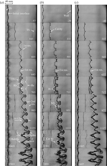
The complete evolutions of SM, TR and ST interfaces interacted by the incident planar shock and the reshocks are clearly captured by the high-speed schlieren photography. Figure 4 gives the interface evolutions and wave patterns for the three cases. The initial time is defined as that when the incident shock wave just arrives at the interface centre. For the SM interface, as presented in figure 4(a), when the incident shock wave propagates along the interface, the transmitted shock wave (TS) and the reflected expansion waves are generated, moving downstream and upstream, respectively. Meanwhile, the phase reversal appears, which is a remarkable feature of the heavy/light interface. The spike grows downstream whereas the bubble evolves upstream, resulting in an extension of the mixing width. When the TS arrives at the endwall, the first reshock (1st res.) propagating upstream is generated. As the first reshock moves from the spike tip to the bubble tip, the reflected shock waves from the spike (Rs) and the bubble (Rb) are generated successively ( $703\ \mathrm {\mu }{\rm s}$). The bubble front becomes flat compared with that before the first reshock, due to the effects of the transverse shock waves (R1) (Motl et al. Reference Motl, Oakley, Ranjan, Weber, Anderson and Bonazza2009; Guo et al. Reference Guo, Zhai, Ding, Si and Luo2020). Later the bubble front becomes sharp and large-scale vortex pairs arise at the spike head (
 $983\ \mathrm {\mu }{\rm s}$). Rs and Rb move downstream and impact the endwall successively, and then form the second reshock (2nd res.), which has two branches. After being impacted by the second reshock, the large-scale structures of the interface deform obviously. The bubble head becomes much sharper, and the spike stem becomes thinner with the growth of the vortex pair.
Sequences of schlieren images of interface evolutions and wave patterns for different initial interface shapes: (a) single-mode, (b) trapezoid and (c) sawtooth. The moments at  $t = 983$, 951 and
 $977\ \mathrm {\mu }{\rm s}$ correspond to the times just before the second reshock impact, and the moments at
 $t = 1123$, 1111 and
 $1117 \mathrm {\mu }{\rm s}$ correspond to the times just after the second reshock impact. IS and TS, the incident and transmitted shock waves; 1st res. and 2nd res., the reshocks reflected from the endwall for the first and the second times; TS1, the transmitted shock wave formed by the first reshock passing through the evolving interface; Rb and Rs, the shock waves reflected from the tips of bubbles and spikes; R1, the transverse shock waves; SD, the small disturbance at the bubble front;
 $h$ and
 $a$, the mixing width and the amplitude of the evolving interface; and
 $T_b$ (
 $T_s$), the bubble (spike) tip thickness, defined as the distance from the leftmost to the rightmost of the bubble (spike) tip. The time unit:
 $\mathrm {\mu }{\rm s}$. Notably, the total width of the interface is 120 mm, whereas the observing window width is 100 mm. Therefore, a quarter of a wavelength near each sidewall cannot be observed.

Figure 4(b) shows the interface evolution and shock patterns of the TR interface. An obvious feature of TR interface evolution is the emergence of cavities. Before reshock, a cavity is formed at the spike tip ( $331\text {--}591\ \mathrm {\mu }{\rm s}$) due to different moving velocities between the vortex pair and the flat part of the spike front. After being impacted by the first reshock, the cavity at the spike tip disappears gradually, while a cavity arises at the bubble tip and develops downstream. A small disturbance that has almost the size of the spanwise width of the bubble front is imposed on the bubble front (
 $951\ \mathrm {\mu }{\rm s}$) owing to the difference in vortex-induced velocities between both sides and the middle of bubble heads. The high-pressure region generated by transverse shock waves (R1) also promotes the formation of the small disturbance. Then, the second reshock impacts the small disturbance, causing a local RM instability at the bubble front. In short, after the first reshock, a small disturbance on the bubble front is seeded, and then the second reshock amplifies the disturbance significantly, generating an obvious cavity.
The interface evolution of the ST interface is presented in figure 4(c). Before reshock, both the bubble and spike fronts are sharp, retaining the original interface characteristics ( $337\text {--}597\ \mathrm {\mu }{\rm s}$). After depositing vorticity on the interface by reshock, the vortex pair at the spike head grows slightly large, whereas the bubble front still keeps sharp. Notably, the ST case looks like an impulsive version of the ‘tilted-rig’ RT experiments of Andrews et al. (Reference Andrews, Youngs, Livescu and Wei2014). There is jetting where there are sharp corners, which can probably be ascribed to the effects of high-order modes. It can be seen that the spikes and bubbles for the three cases exhibit their own features after reshock. The vortex pairs at spike heads dominate the spike deformation. The vortex pairs of the SM and TR interfaces develop very quickly, causing the spike heads of the two cases to have a larger spanwise size. At late times, the spike morphologies for both cases are quite homologous. The effects of mass conservation become important at late times because the spike gets close to the endwall. To maintain the mass conservation, the bubbles of SM and ST interfaces tend to develop upstream, while the bubbles of the TR interface tend to grow in the spanwise direction since the cavity on bubble tips inhibits bubbles from growing upstream. For all cases, the bubble tips get increasingly thick, and local chaotic mixing at bubble tips seems to arise at late times, which is ascribed to rapid growths of small-scale disturbances on bubble tips. The small-scale disturbances promote the bubble tips to develop upstream and make bubbles of the SM interface incrementally sharp. Eventually, the bubble morphology of the SM interface becomes nearly the same as that of the ST interface at late stages.
3.2. Interface mixing width before and after reshock
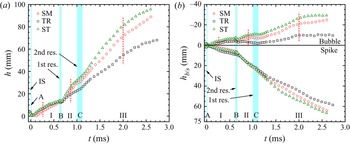
Figure 5(a) shows the evolution of the mixing width  $h$ changing with time for the three cases. In experiments, the interface mixing width is measured from the middle position of the bubble tip to the rightmost side of the spike tip, since the spike tip thickness varies little before and after reshock and has very limited effects on the whole mixing width (taking the SM interface as an example, half the spike tip thicknesses are 1.52 mm, 1.96 mm and 2.39 mm at
 $t = 383\ \mathrm {\mu }{\rm s}$,
 $703\ \mathrm {\mu }{\rm s}$ and
 $2603\ \mathrm {\mu }{\rm s}$, respectively). Six stages can be identified depending on the shock arrival time. The periods A, B and C stand for those during the shock waves passing through the interface, and the periods I, II and III stand for those when the shock waves move away from the distorted interface. As displayed in figure 5(a), when the incident shock propagates across the interface, the mixing width decreases due to shock compression and phase reversal (stage A). The spike growth rate for the SM interface is the smallest due to less deposition of baroclinic vorticity, resulting in the longest phase reversal duration. In stages I, II and III, the mixing width grows first linearly and then nonlinearly. Owing to the weak intensity of the second reshock, the growth of mixing widths in stage C seems not to be influenced. The interface shape has limited effects on the mixing width growth tendency but determines the ranking of the growth rates. After the first reshock, the ST mixing width has the largest growth rate, while the TR mixing width has the smallest one.
Time variation of the overall mixing width (a) and the widths of spikes and bubbles (b) for the three cases. The arrows represent the times when the incident shock (IS), the first reshock (1st res.) and the second reshock (2nd res.) just arrive at the interface. The red dashed lines in panels (a) and (b) denote the beginning time of the nonlinear growth of the whole mixing width, and the corresponding time for the bubble width growth, respectively.

The variations of the spike width ( $h_s$) and the bubble width (
 $h_b$) versus time for the three cases are displayed in figure 5(b). Here
 $h_s$ (
 $h_b$) is defined as the distance from the rightmost side of the spike tip (the middle position of the bubble tip) to the position of an unperturbed interface, which is used as the reference surface. After the phase reversal, the TR spike width has the largest growth rate, while the SM spike width has the smallest one. The spike growth difference is ascribed to the different vorticity intensity of the spike head. After the first reshock, the spike growths for different interface shapes become nearly the same before
 $t \approx 1.1$ ms. But after the second reshock completely passes through the whole interface, the growth difference begins to appear. Notably, the spike and the bubble widths have the same growth ranking in stage III. As displayed in figure 4, the spanwise size of the TR spike (bubble) head is the largest, while the counterpart of the ST spike (bubble) head is the smallest. From continuity, the growth rate of the spike (bubble) width will decrease due to the increased spanwise spike (bubble) size. In addition, for the TR interface, the cavity structure at the bubble tip can inhibit the growth of bubble and spike widths (the vorticity on the cavity mainly induces a velocity in the upstream direction for the spike). Therefore, at late times, the TR spike and bubble widths have the smallest growth rates, while the ST spike and bubble widths have the largest ones. Interestingly, the growth between the bubble width and whole mixing width exhibits highly similar characteristics (the same growth rate ranking and the similar growth tendency). As a result, the evolution behaviours of bubble widths determine the development behaviours of the whole mixing width.
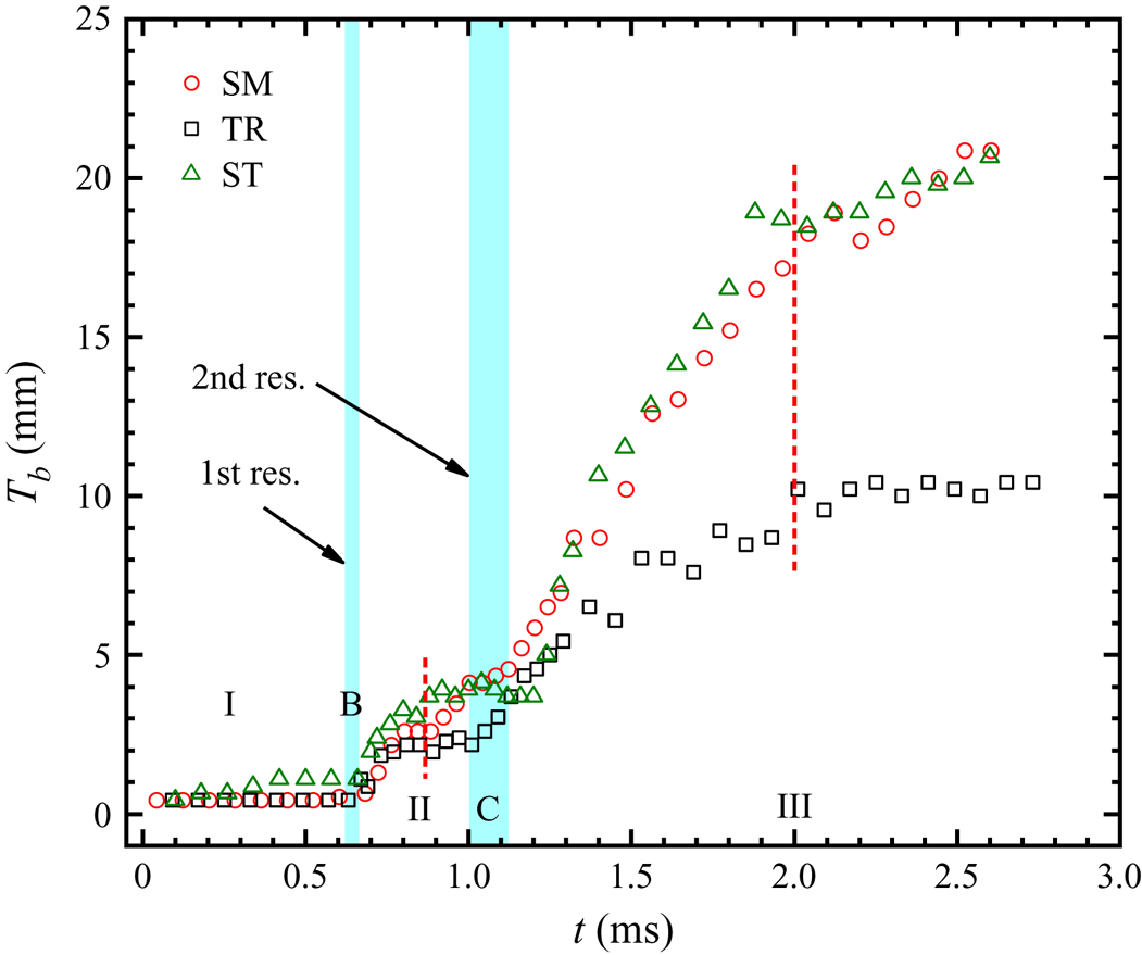
In experiments, as shown in figure 4, the bubble tip thickness ( $T_b$) increases much more quickly than the spike tip thickness (
 $T_s$). Figure 6 shows the variation of the bubble tip thickness
 $T_b$ versus time for the three cases. Surprisingly, compared with the growth characteristics of the bubble widths presented in figure 5(b), the growth behaviours of the bubble tip thickness for the three cases after reshock are very consistent with that of the whole bubbles. The diffusion of gases at both sides of the interface can make the bubble tip thicker. In addition, as time elapses, small-scale disturbances on the bubble tip develop gradually, which can also result in an increasing bubble tip thickness. However, in the shock–interface interactions, Brouillette & Sturtevant (Reference Brouillette and Sturtevant1994) pointed out that gas diffusion is much slower than the growth rate of the small-scale disturbances on the interfaces. As shown in figure 6, before the first reshock, the bubble tip thickness varies little, which verifies that the gas diffusion is indeed insignificant in such a short time. After the reshock, the bubble tip thickness grows quickly, and has a growth tendency similar to the bubble width. Therefore, the rapid growth of small-scale disturbances is the main reason for the increasing bubble tip thickness. Owing to the similarity between the growths of the bubble tip thickness and the bubble width, the developments of large-scale bubbles are closely related to the growth behaviours of the small-scale disturbances on the bubble tip, and the dominant mechanism of small-scale disturbance growths is probably consistent with that of large-scale bubbles.
Variation of the bubble tip thickness versus time for the three cases.

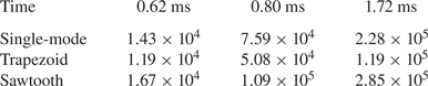
The Reynolds number is calculated to characterize the variable-density flow. The Reynolds number is given by  $Re=a\dot {a}/\nu _{mix}$, where
 $a$ is the interface amplitude,
 $\dot {a}$ is the amplitude growth rate and
 $\nu _{mix}$ is the mixed kinematic viscosity of gases. The
 $\nu _{mix}$ value can be found using
 $(\mu _1+\mu _2)/(\rho _1+\rho _2)$ (Mohaghar et al. Reference Mohaghar, Carter, Musci, Reilly, McFarland and Ranjan2017), where
 $\mu _1$ and
 $\mu _2$ (
 $\rho _1$ and
 $\rho _2$) are the viscosities (densities) of the mixed gases at the left and right side of the interface, respectively. According to one-dimensional gas dynamics and property relations, the values of
 $\nu _{mix}$ for three stages (before the first reshock, and after the first and second reshocks) are determined to be
 $4.76 \times 10^{-6}$,
 $3.35 \times 10^{-6}$ and
 $3.05 \times 10^{-6}$, respectively. Based on the values of
 $\nu _{mix}$, the Reynolds numbers at three typical moments are calculated, as listed in table 2. One can find that for the ST case, the Reynolds number is larger than that in other cases, while for the TR case, the Reynolds number is the smallest.
The Reynolds numbers at three typical moments.

4. Theoretical predictions
4.1. Perturbation growth before reshock
For the heavy/light case, the interface amplitude first experiences a linear growth stage after the phase reversal. Meyer & Blewett (Reference Meyer and Blewett1972) proposed a theoretical model (the MB model) to predict the linear growth of an SM interface with a small initial amplitude. The MB model can be described as
 \begin{equation} V^{MB}_{0}=k|A^{+}|\Delta V_1\frac{a_0+a_{0}^{+}}{2}, \end{equation}
where  $k = 2{\rm \pi} /\lambda$ is the wavenumber and
 $a_{0}^{+} = a_0(1-\Delta V_1/U_i)$ is the post-shock amplitude, with
 $U_i$ being the incident shock velocity. Table 3 shows the comparison between the experimental linear growth rates and the theoretical predictions obtained from the MB model, which has a good prediction of the linear growth rates for the SM interface. Since the initial interfaces with quasi-single-mode shapes can be described by the Fourier expansions with a dominant mode, the TR and the ST interfaces have linear growth rates very similar to the SM interface. As a result, the MB model can also estimate the linear growth of TR and ST interfaces.
The experimental and theoretical amplitude linear growth rates, with  $V^{E}_{0}$ the average experimental linear growth rate from three runs of each case, and
 $V^{MB}_{0}$ the theoretical prediction obtained from the MB model. The unit of velocities is
 ${\rm m}\ {\rm s}^{-1}$.

In the nonlinear stage, there are several models to predict the amplitude growth of an SM interface. By matching the 2-D weakly nonlinear solution (Zhang & Sohn Reference Zhang and Sohn1997) at early times and the potential asymptotic solutions (Alon et al. Reference Alon, Hecht, Ofer and Shvarts1995) at late times, Sadot et al. (Reference Sadot, Erez, Alon, Oron, Levin, Erez, Ben-Dor and Shvarts1998) proposed an empirical nonlinear model (the SEA model). For large ( $A \geqslant 0.5$) and small (
 $A \rightarrow 0$) Atwood numbers, this model gives different predictions due to adopting different potential solutions. Dimonte & Ramaprabhu (Reference Dimonte and Ramaprabhu2010) constructed an empirical nonlinear model (the DR model), which gives a good prediction of their numerical results. This model considers the variation of the initial amplitudes and is also applicable to cases of various Atwood numbers. In the spirit of Layzer (Reference Layzer1955), Zhang & Guo (Reference Zhang and Guo2016) studied the asymptotic large-time behaviour of the RM instability by considering the governing equations for incompressible, inviscid and irrotational fluids with arbitrary density ratios in two dimensions, and proposed a model (the ZG model) to capture the nonlinear behaviours of bubbles and spikes. The ZG model can be expressed as
 \begin{equation} V_{b/s}^{ZG}(t)=V_0\frac{1}{1+\alpha kV_0t}, \end{equation}
where
 \begin{equation} \alpha=\frac{3}{4}\frac{(1+A^{+})(3+A^{+})}{[3+A^{+}+\sqrt{2}(1+A^{+})^{1/2}]}\, \frac{[4(3+A^{+})+\sqrt{2}(9+A^{+})(1+A^{+})^{1/2}]} {[(3+A^{+})^{2}+2\sqrt{2}(3-A^{+})(1+A^{+})^{1/2}]}, \end{equation}
with a positive Atwood number for bubbles and its negative counterpart for spikes. These models have been proved to be effective in capturing the asymptotic behaviours of single-mode and quasi-single-mode interfaces with light/heavy configurations (Jacobs & Krivets Reference Jacobs and Krivets2005; Liang et al. Reference Liang, Zhai, Ding and Luo2019). However, for a heavy/light interface, it is still necessary to assess the validity of the existing nonlinear models.
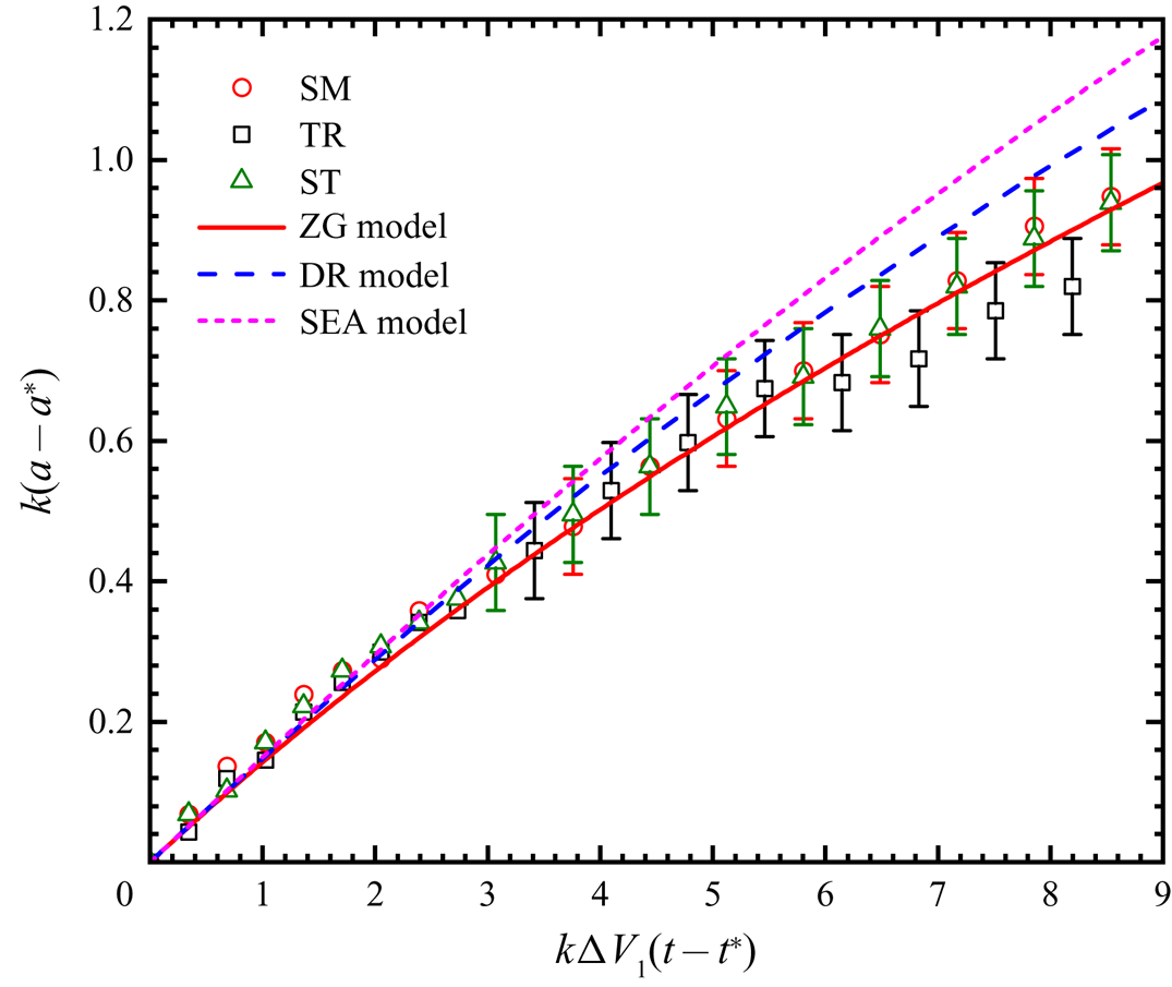
Figure 7 shows the comparison between the experimental amplitude growth and the theoretical predictions obtained from three nonlinear models. Similar to previous work considering the reshock (Balakumar et al. Reference Balakumar, Orlicz, Ristorcelli, Balasubramanian, Prestridge and Tomkins2012), the wavenumber  $k$ and the jump velocity
 $\Delta V_1$ are selected for normalizing the time
 $t$, which has a dimensionless form
 $k\Delta V_1(t-t^{*})$, with
 $t^{*}$ the time when the phase reversal is just completed. The amplitude is scaled by
 $k(a-a^{*})$, where
 $a^{*}$ is the amplitude at
 $t^{*}$. As presented in figure 7, the three shapes still have very similar amplitude growth rates at the nonlinear stage, which indicates that the effects of quasi-single-mode interface initial shapes are weak even when the nonlinear feature occurs. Both the SEA and DR models overestimate the nonlinear growth rates of the three shapes, whereas the ZG model can well capture the nonlinear behaviours for all cases, which verifies that, for the heavy/light single-mode and quasi-single-mode interfaces, the ZG model still gives the most satisfactory prediction of the nonlinear growth rate, which is similar to the previous work for the SM interface with a light/heavy configuration (Liu et al. Reference Liu, Liang, Ding, Liu and Luo2018).
Comparisons of experimental and theoretical growth rates in the linear and nonlinear stages before reshock. The symbols denote the experimental results, and the lines represent theoretical predictions from the ZG model (Zhang & Guo Reference Zhang and Guo2016), the DR model (Dimonte & Ramaprabhu Reference Dimonte and Ramaprabhu2010) and the SEA model (Sadot et al. Reference Sadot, Erez, Alon, Oron, Levin, Erez, Ben-Dor and Shvarts1998).

4.2. Mode analysis
The mode evolution of different interfaces is useful for understanding the interface deformation and growths for different cases. The mode information (amplitude, phase and frequency) of interfaces can be obtained by fast Fourier transform (FFT) (Guo et al. Reference Guo, Zhai, Ding, Si and Luo2020). The FFT requires the interface shape to be a single-valued function. As shown in figure 4, there are no evident vortex structures for the SM and the ST interfaces before reshock and even for a period after the first reshock strikes the interface. For the TR interface, very small vortex pairs are formed at the spike head at  $t\approx 331\ \mathrm {\mu }{\rm s}$, i.e. the TR shape is not a single-valued function at this moment. However, for comparison, the TR interface is also analysed through FFT before the further development of vortex pairs, and the mode information of the interface is obtained.
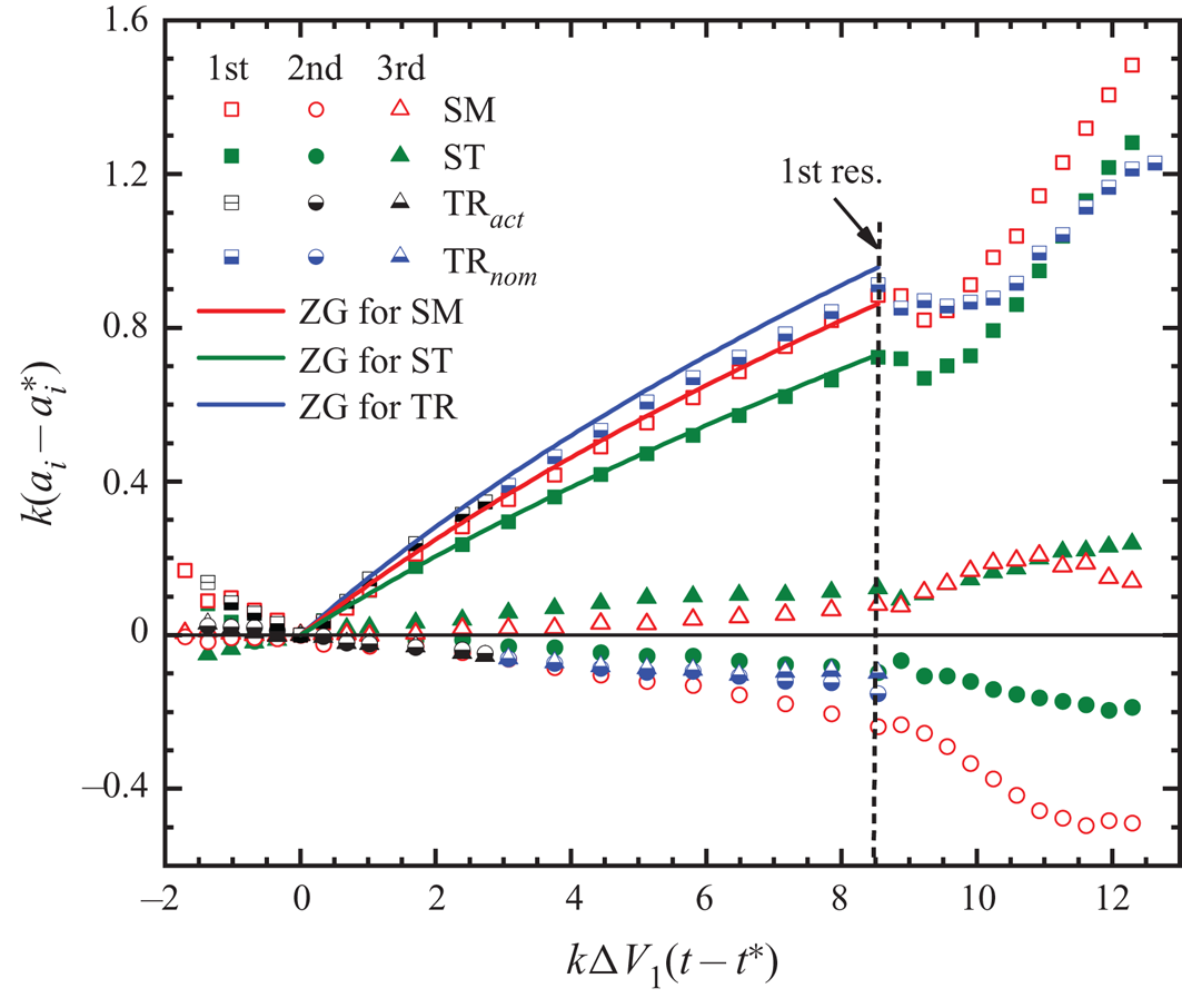
Figure 8 shows the amplitude growths of the first three modes versus time for the three cases. The data of the TR interface use symbols in two colours. The data with symbols in black (blue) colour are obtained before (after) the vortex pair arises, thus they are actual (nominal). Before the first reshock, the TR interface has the largest amplitude growth rate of the first mode, while the ST interface has the smallest one. This is consistent with the initial mode distribution where the first mode amplitude of the TR interface is 114.6 % of the whole amplitude, whereas the counterpart of the ST interface is only 81.1 %. Because a large-amplitude first mode will generate a large-amplitude second harmonic mode, the growth rate of the second harmonic mode for the ST interface is smaller than that of the other two cases. Previous work indicated that the second mode with a large amplitude could flatten the bubble front (Guo et al. Reference Guo, Zhai, Ding, Si and Luo2020). In the present work, the amplitude of the second harmonic mode for the ST interface is small so that the bubble tip always remains sharp. Unlike the other two cases, the third harmonic mode of the TR interface is out of phase with the first mode, which preserves the initial phase characteristics displayed in (2.1).
Comparisons of amplitude growths of the first three modes for three shapes. The symbols represent the experimental results, and the lines represent the theoretical predictions of the ZG model (Zhang & Guo Reference Zhang and Guo2016). Here  ${\rm TR}_{act}$ and
 ${\rm TR}_{nom}$ denote the actual and the nominal mode amplitudes of the TR interface, respectively;
 $a_{i=1, 2, 3}$ represent the amplitudes of the first, second and third modes, respectively; and
 $a_i^{\ast }$ is the corresponding mode amplitude at
 $t^{\ast }$.

After the first reshock, the first mode amplitude grows rapidly, which is the main reason for the significant increase in the amplitude of the entire interface for the three cases after reshock. For the SM interface, the amplitude of the second harmonic mode is enhanced prominently. After the first reshock, the transverse shock waves impact the interface, generating additional second harmonics (Guo et al. Reference Guo, Zhai, Ding, Si and Luo2020). The increasing amplitude of the second harmonic modes causes the bubble front to be flatter (figure 4a,  $t = 703\ \mathrm {\mu }{\rm s}$) than that before the first reshock (figure 4a,
 $t = 643\ \mathrm {\mu }{\rm s}$). From
 $k\Delta V_1(t-t^{*}) \approx 11$, the small-scale disturbances on the bubble tip cannot be ignored and grow rapidly, which leads to the growth stagnation for the second harmonic mode. However, for the ST interface, the amplitude of the second harmonic mode is still relatively small despite the reshock impact, resulting in much sharper bubble tips of the ST interface after reshock than those of the SM and TR cases.
The ZG model can be used to evaluate the amplitude growth of the first mode for the three shapes. As displayed in figure 8, the ZG model agrees very well with experimental results for the three cases. This consolidates the conclusion that, for the quasi-single-mode interfaces, the first mode will dominate the interface evolution before reshock, and the effects of high-order modes are weak. As a result, the overall amplitude growths for the three cases are very similar and can be predicted by the ZG model, as shown in figure 7. Additionally, for the TR interface, even though vortex pairs arise at the spike head, the good agreement between the ZG model and the experimental results indicates that the vortex pairs have limited effects on the amplitude growth of the first mode.
The amplitude ratios of the first three modes to the whole interface before and after reshock are listed in table 4. The predominance of the first mode seems not to be changed after reshock and lasts almost until the second reshock arrives. After the second reshock, as the vortices, especially the vortex pairs at the spike head, develop, the interface deforms significantly, so that the first mode cannot be obtained by FFT. At this time, the first mode may be more suitable to be called the energy-containing mode due to receiving most of the energy from shocks. Notably, as shown in figure 5, the growth trends of mixing widths in stages I, II and III are very similar (the mixing width experiences linear and nonlinear growths in sequence); thus, it is believed that the first mode always dominates the interface evolution even though the interface deforms obviously and small-scale disturbances have developed. This also gives the prospect that the theories proposed for the singly shocked case might also be applicable to the case after reshock for single-mode and quasi-single-mode interfaces.
The amplitude ratios of the first three modes to the whole interface at three typical moments. Here  $t_i$,
 $t_b$ and
 $t_a$ represent the moments before the incident shock, and before (
 $k\Delta V_1(t-t^{*}) \approx 8.5$) and after (
 $k\Delta V_1(t-t^{*}) \approx 12$) the first reshock, respectively. The results of the second and the third modes for the TR interface are omitted.

4.3. Mixing width growths
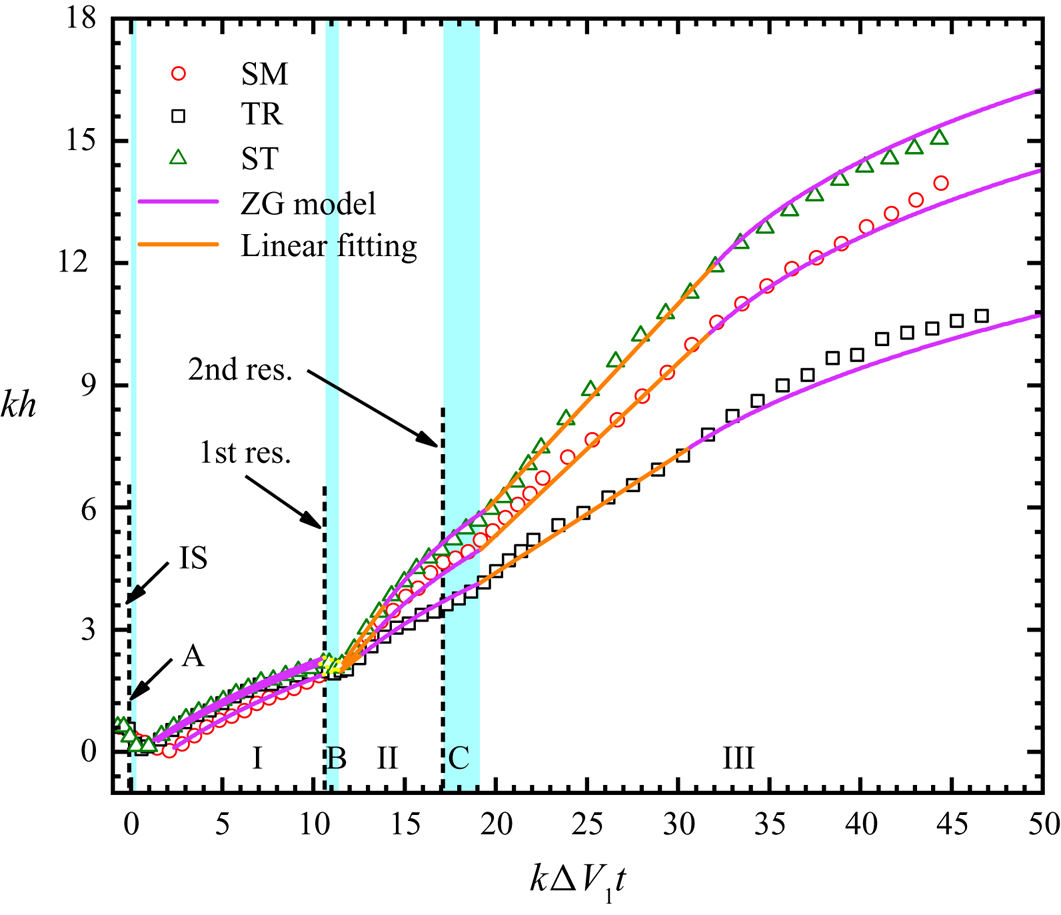
Figure 9 shows the dimensionless time variations of mixing widths for the three cases. The linear growth rates after the first and second reshocks are obtained through linear fittings, and the detailed values of growth rates are listed in table 5. Although the first mode is still dominant after reshock, large differences in growth rates among the three cases appear, which is different from the findings in previous studies (Leinov et al. Reference Leinov, Malamud, Elbaz, Levin, Ben-Dor, Shvarts and Sadot2009; Jacobs et al. Reference Jacobs, Krivets and Tsiklashvili2013; Mohaghar et al. Reference Mohaghar, Carter, Musci, Reilly, McFarland and Ranjan2017, Reference Mohaghar, Carter, Pathikonda and Ranjan2019). In the work of Leinov et al. (Reference Leinov, Malamud, Elbaz, Levin, Ben-Dor, Shvarts and Sadot2009) and Jacobs et al. (Reference Jacobs, Krivets and Tsiklashvili2013), the turbulent transition has probably been completed after reshock, causing the mixing width growth to lose the memory of interface shapes at the time of reshock. In the studies of Mohaghar et al. (Reference Mohaghar, Carter, Musci, Reilly, McFarland and Ranjan2017, Reference Mohaghar, Carter, Pathikonda and Ranjan2019), the growth in mixing widths is predominantly driven by the largest mode of the initial perturbation, while smaller modal contents are insignificant and can be ignored. However, in the present work, the interface is still approximately single-scale after reshock, and high-order modes on the interface are more comparative to the fundamental mode. The influences of high-order modes are amplified by reshock, eventually resulting in different growth behaviours for different shapes.
Comparisons between experiments and model predictions for the mixing widths. The symbols denote the experimental results, the orange lines represent the results from linear fittings, and the magenta lines represent the theoretical predictions of the ZG model (Zhang & Guo Reference Zhang and Guo2016).

The velocities and parameters before and after reshock. Here  $V_{1r}$ and
 $V_{2r}$ are the mixing width growth rates after the first and the second reshock;
 $V_{b}$ is the mixing width growth rate just before the first reshock;
 $V_{a}$ is the mixing width growth rate induced by the first reshock (all these data are obtained by averaging the corresponding values from three experimental runs);
 $\beta _e$ is the experimental parameter calculated from the Charakhch'yan model; and
 $R_{21}\ (= V_{2r}/V_{1r})$ is the ratio of the linear width growth rate after the first reshock to that after the second reshock. The unit of velocities is
 ${\rm m}\ {\rm s}^{-1}$.

It has been demonstrated that, for a single-scale interface, only odd-order modes determine the whole interface mixing width, while even-order modes have no effect on the whole mixing width growth (Luo et al. Reference Luo, Liang, Si and Zhai2019; Guo et al. Reference Guo, Zhai, Ding, Si and Luo2020). At the time of the first reshock arrival, the major odd-order modes for the SM and ST interfaces are nearly in phase, while the counterpart for the TR interface is almost out of phase, implying that, after reshock, for the SM and the ST interfaces, the superposition of amplitudes of major odd-order modes promotes the growth of the whole mixing width, but for the TR interface, the amplitudes of major odd-order modes are offset, inhibiting the growth of the whole mixing width. As a result, after reshock, the SM and ST interfaces have larger width growth rates, while the TR interface possesses a relatively small one. Notably, the width growth rate of the ST interface is greater than that of the SM interface. As shown in figure 8, the amplitude growth rates of the first mode for the ST and SM interfaces are nearly the same, but the ST interface has a smaller amplitude of the first mode. Thus, in comparison with the SM interface, the development of high-order modes of the ST interface plays a greater role in promoting the increase of amplitudes.
To evaluate the reshocked mixing width growth rate for the case where the perturbation growth has been nonlinear before reshock, Charakhch'yan (Reference Charakhch'yan2000) built a model (the Charakhch'yan model) with the following expression:
 \begin{equation} V_{1r}=V_a+V_b=\beta A^{+}_r\Delta V_{1r}+V_b. \end{equation}
Here  $V_{1r}$ and
 $\Delta V_{1r}$ are the mixing width growth rate after reshock and the jump velocity induced by reshock, respectively;
 $V_a$ is the growth rate induced by reshock;
 $V_b$ is the growth rate before reshock;
 $A^{+}_r$ is the post-reshock Atwood number; and
 $\beta$ (
 ${=}1.25$) is an empirical parameter determined by numerical simulations. The Charakhch'yan model was proposed for an SM interface with initial heavy/light configurations, whereas the value of
 $\beta$ has not been validated by experiments so far, due to the lack of reshock experiments with an initially well-defined 2-D SM interface at the heavy/light configuration.
Our experiments with initial well-defined heavy/light 2-D interfaces give a good chance to verify the model value of  $\beta$. As presented in table 5, the value of
 $\beta _e$ obtained from experiments is smaller than the model value
 $\beta = 1.25$. In the work of Charakhch'yan (Reference Charakhch'yan2000), numerical simulations were carried out with
 $h_{1r}/\lambda = 0.09\text {--}0.88$, where
 $h_{1r}$ is the mixing width just before the first reshock, and values of
 $\beta$ in the range of 0.53–1.5 were obtained. To match the linear growths in the case of
 $h_{1r}\sim \lambda$ (i.e. the perturbation growth at the time of the first reshock arrival is in the strongly nonlinear stage), Charakhch'yan averaged the values of
 $\beta$ corresponding to
 $h_{1r}/\lambda$ in the range of 0.62–0.88, and obtained the average
 $\beta = 1.25$. In our present work, when the first reshock arrives at the interface, the perturbation growths for the three cases are in the weakly nonlinear stage (
 $h_{1r}/\lambda \approx 0.34$), which makes
 $\beta _e$ smaller than
 $\beta =1.25$. Our
 $\beta _e$ values for the three cases are listed in table 5, nearly within the range of
 $\beta = 0.53\text {--}1.5$ obtained from numerical simulations, even though the initial conditions in the present experiments are quite different from those in the simulations of Charakhch'yan, where strong incident shocks and high Atwood numbers (
 $|A|=1$, an aluminium/vacuum interface) were set.
The mixing width growth rate ( $V_{2r}$) after the second reshock is smaller than
 $V_{1r}$, which is different in that
 $V_{1r}$ is larger than the initial growth rate
 $V_0^{E}$. The second reshock is weak so that it hardly induces large growth rates, but it still cancels out the nonlinearity and makes the mixing width grow linearly. The ratios (
 $R_{21}$) of
 $V_{2r}$ to
 $V_{1r}$ for the three cases are listed in table 5. The
 $R_{21}$ value seems insensitive to interface shapes, and the average value of
 $R_{21}$ for the three cases is about 0.81. Thus, if
 $V_{1r}$ is theoretically determined,
 $V_{2r}$ can be empirically obtained by
 $V_{2r} = 0.81V_{1r}$.
The transition time from the linear to the nonlinear growths, i.e. the linear growth duration ( $\hat {t}$), should be determined before predicting the nonlinear growths of mixing widths. From the dimensional argument, a length scale and a velocity are required to define
 $\hat {t}$. Based on the previous singly shocked experiments of single-mode or quasi-single-mode interfaces (Jacobs & Krivets Reference Jacobs and Krivets2005; Morgan et al. Reference Morgan, Aure, Stockero, Greenough, Cabot, Likhachev and Jacobs2012; Guo et al. Reference Guo, Ding, Luo and Zhai2018; Liu et al. Reference Liu, Liang, Ding, Liu and Luo2018; Liang et al. Reference Liang, Zhai, Ding and Luo2019) and our present work, the linear growth duration after the impact of the incident shock can be expressed in the form
 \begin{equation} \hat{t}\approx\frac{0.5}{kV_0}=\frac{1}{4{\rm \pi}}\frac{\lambda}{V_0}, \end{equation}
where  $V_0$ is the linear growth rate. One can find that, for the singly shocked case, the wavelength
 $\lambda$ as the length scale and
 $V_0$ as the velocity are appropriate for constructing the expression for
 $\hat {t}$. For the reshock situation, the linear growth rates
 $V_{1r}$ and
 $V_{2r}$ are both different for the three cases, thus, (4.5) would give different
 $\hat {t}$ for different shapes. This is in contradiction with the experimental findings that
 $\hat {t}$ is independent of interface shapes. As a result, (4.5) is insufficient to predict
 $\hat {t}$ for the reshock case.
According to (4.1) and (4.4), the mixing widths for RM instability satisfy the following form:
 \begin{equation} h\sim |\Delta V|t. \end{equation}
Therefore, the pre-shock mixing width ( $h_0$) and the jump velocity (
 $\Delta V$) might be suitable for determining
 $\hat {t}$. However, as shown in figure 5(a), the linear growth duration after the second reshock is insensitive to
 $h_{2r}$ (the mixing width prior to the second reshock), thus, the preshock mixing width is also not suitable as the length scale. Finally, we choose the initial wavelength
 $\lambda$ and the jump velocity
 $\Delta V$ to construct the expression of
 $\hat {t}$, which can be given by
 \begin{equation} \hat{t}=\frac{\lambda}{|\Delta V|}\delta, \end{equation}
where  $\delta = 3/(2{\rm \pi} )$. The theoretical
 $\hat {t}$ obtained from (4.7) are 0.18 ms, 0.24 ms and 0.89 ms after the incident shock, the first and the second reshocks, respectively, which are quite close to the experimental results (0.18 ms, 0.23 ms and 0.9 ms, respectively).
Equation (4.7) has a similar form to that obtained by Mikaelian (Reference Mikaelian2011), who studied the transition time of turbulent mixing layer widths from the linear to the power-law growth. The preshock mixing width  $h_0$ was used as the length scale, and the expression was given as
 $\hat {t}=(h_0/{|\Delta V|})\delta$, with
 $\delta \approx 6$. However, the model of Mikaelian (Reference Mikaelian2011) cannot predict our linear growth duration, probably because the interfaces still remain approximately single-scale after reshock. Both models for
 $\hat {t}$ in this work and Mikaelian (Reference Mikaelian2011) indicate that the jump velocity
 $\Delta V$ is significant in determining the linear growth duration.
The ZG model is used to predict the nonlinear growths after reshock because of the predominance of the first mode. As presented in (4.2), when  $t\rightarrow 0$, the ZG model is matched by
 $V_0$, i.e. the growth given by the ZG model is approximately linear at the initial stage. Previous work showed that the dimensionless linear growth time (
 $kV_0t$) of the ZG model is about 0.5 (Liu et al. Reference Liu, Liang, Ding, Liu and Luo2018; Liang et al. Reference Liang, Zhai, Ding and Luo2019), and after
 $kV_0t = 0.5$, the nonlinearity begins to be gradually evident. As a result, when adopting the ZG model to predict the reshocked nonlinear growth of mixing widths, the transition time between the linear and the nonlinear growth should be
 $0.5/[kV_{{1(2)r}}]$ earlier than
 $\hat {t}$. Notably, as the growth transition from linear to nonlinear is not instantaneous, this advance of the transition time is just right to achieve a smooth connection between the linear and the nonlinear growth through the ZG model.
Figure 9 shows the comparison between the experimental mixing widths and the theoretical predictions. The experimental linear growth rates obtained from the linear fitting are applied as the initial start-up growth rates to ensure the prediction reliability of the ZG model. One can find that the ZG model can well predict the reshocked nonlinear growth rates, which indicates that, for the initial single-mode and quasi-single-mode interfaces, the first mode still has predominant effects on the interface evolution. As a result, the growth behaviours after reshock have strong similarities to that in the singly shocked case.
5. Conclusions
Experimental studies on the Richtmyer–Meshkov (RM) instability of heavy/light interfaces upon reshock are conducted, considering typical quasi-single-mode interfaces with trapezoid and sawtooth shapes in comparison with the single-mode interface. The reflection distance is specifically selected to ensure that the distorted interface at the first reshock arrival is in the weakly nonlinear stage, where the interface shape still maintains a single-valued function before distinct vortex pair generation. In experiments, well-defined initial interfaces are generated by the soap-film technique, and clear interface morphologies and wave patterns are captured by high-speed schlieren photography.
The development of interface morphologies exhibits a strong memory of initial shapes. The heads of bubbles and spikes of the trapezoid interface tend to expand in the spanwise direction, while the counterparts of the sawtooth interface tend to remain sharp and develop horizontally. For the single-mode interface, the spike develops gradually, with its shape similar to that of the trapezoid interface, whereas its bubble morphology evolves like that of the sawtooth interface. The vortex pairs at spike heads dominate the spike deformation, while the effects of mass conservation and the growths of small-scale disturbances on bubble tips play a great role in the bubble evolution. Before reshock, the amplitude growth rates of the single-mode and quasi-single-mode interfaces are nearly the same, which indicates that the first mode is completely dominant, while the effects of high-order modes can be ignored. However, the reshock amplifies the effects of high-order modes, resulting in significant interface shape dependence of mixing width growths, which is different from the findings in previous experiments (Leinov et al. Reference Leinov, Malamud, Elbaz, Levin, Ben-Dor, Shvarts and Sadot2009; Jacobs et al. Reference Jacobs, Krivets and Tsiklashvili2013; Mohaghar et al. Reference Mohaghar, Carter, Musci, Reilly, McFarland and Ranjan2017, Reference Mohaghar, Carter, Pathikonda and Ranjan2019).
The superposition of amplitudes of major odd-order modes promotes the mixing width growth rate for the single-mode and sawtooth interfaces, while the offset of amplitudes of major odd-order modes inhibits the mixing width growth rate for the trapezoid interface. Compared with the single-mode interface, the development of high-order modes of the sawtooth interface plays a greater role in promoting the increase of amplitudes, so that the sawtooth interface has the largest mixing width growth rate, while the trapezoid interface has the smallest one. The ranking of width growth rates of bubbles and spikes shows the same dependence on the interface shape as that of the overall mixing width growth rate. The bubble width evolution behaviours determine the whole mixing width evolution behaviours. The developments of large-scale bubbles are closely related to the growth behaviours of small-scale disturbances on the bubble tip.
The complete perturbation growths of different interfaces before and after reshock are studied experimentally and theoretically. The impulsive model proposed by Meyer & Blewett (Reference Meyer and Blewett1972) and the nonlinear model (the ZG model) formulated by Zhang & Guo (Reference Zhang and Guo2016) are proved to be effective for predicting the linear and nonlinear growth rates before reshock, respectively. The experimental parameter  $\beta$ reflecting the linear growth of mixing widths after the first reshock is smaller than the model value of Charakhch'yan (Reference Charakhch'yan2000), because the amplitude growths are in different stages when the first reshock arrives. Based on dimensional analysis, an empirical model describing the transition time from the linear to the nonlinear growth is constructed. The ZG model is also effective for predicting the reshocked nonlinear growth rates of mixing widths. This indicates that, after reshock, even though high-order modes can affect the growth rate, the first mode still dominates the interface growth trend, causing the growth behaviours after reshock to have strong similarities to that of the singly shocked case.
Acknowledgements
The authors would like to thank Professor Z. Zhai and Mr Z. Zhou for invaluable discussions on the theoretical analysis.
Funding
This work was partially supported by the National Natural Science Foundation of China (nos. 12027801, 11625211, 91952205 and 11621202), the Youth Innovation Promotion Association CAS (no. 2018491) and the Fundamental Research Funds for the Central Universities.
Declaration of interests
The authors report no conflict of interest.