


1 Introduction
The term ‘mild-slope equations’ refers to a collection of approximations for the scattering of linear surface waves on water of variable depth that has been developed over a period of time. The common factors linking the approximations is that they focus attention solely on progressing waves and they use an averaging method to remove the dependence of the motion on the vertical coordinate, thereby significantly reducing the scale of a typical scattering problem. The approximation process requires the bed slope to be ‘mild’ in the sense that
 $$\begin{eqnarray}|\unicode[STIX]{x1D735}h/kh|\ll 1\end{eqnarray}$$
at each location, where  $h$ is the water depth and
 $k$ the corresponding wavenumber.
Berkhoff (Reference Berkhoff1973, Reference Berkhoff1976) derived what is now known as the ‘mild-slope equation’ (MSE), which may also be found in Jonsson & Brink-Kjaer (Reference Jonsson and Brink-Kjaer1973), Smith & Sprinks (Reference Smith and Sprinks1975) and Lozano & Meyer (Reference Lozano and Meyer1976). Other derivations have been given since by Kirby (Reference Kirby1986) and Miles (Reference Miles1991), while Chamberlain & Porter (Reference Chamberlain and Porter1995) and Porter & Staziker (Reference Porter and Staziker1995) produced a more accurate version of the MSE, referred to as the ‘modified mild-slope equation’ (MMSE), at the expense of increased complication. However, Porter (Reference Porter2003) devised a transformation that considerably simplified the application of the MMSE.
All of the derivations mentioned so far employed the velocity potential formulation to describe the fluid motion. An alternative approach that uses a vector streamfunction instead of a potential to represent the velocity field was introduced by Kim & Bai (Reference Kim and Bai2004) and led to the ‘complementary mild-slope equation’ (CMSE). The inevitable complexity of the vector CMSE was somewhat alleviated by Toledo & Agnon (Reference Toledo and Agnon2010) who reduced it to a scalar equation.
The mild-slope equations may be regarded as extensions of the long-standing shallow water equation (SWE; see, for example, Lamb (Reference Lamb1932) or Stoker (Reference Stoker1957)). In the long wave limit ( $kh\ll 1$), an approximation can be invoked in which the pressure distribution in the fluid may be regarded as hydrostatic. This simplifies the vertical structure of the motion and an integration may be carried out, leading to an equation that involves only the horizontal coordinates. The mild-slope equations are attempts to obtain the same simplification for all wavelengths. However, as there is no direct derivation corresponding to that of the SWE for general values of
 $kh$, the dependence of the variables on the vertical coordinate has to be imposed and integration used to smooth out the effect of this approximation. A weak solution of the governing equations is therefore obtained, in the spirit of Galerkin’s method. In effect, the process replaces a vertical filament of fluid by a single aggregate particle lying at the mean free surface. Clearly, no attempt is made to reproduce the vertical motion within the fluid, except in a broad overall sense.
Mild-slope formulations have been applied to other areas, such as surface wave scattering by floating ice (see Porter & Porter Reference Porter and Porter2004), and they have been extended to ‘multi-mode’ approximations (see, for example, Massel (Reference Massel1993) and Athanassoulis & Belibassakis (Reference Athanassoulis and Belibassakis1999)) in which evanescent waves are combined with the travelling mode to increase the accuracy of the scattering process to any desired level.
This investigation returns to the original aim of deriving a single equation to estimate the scattering of progressing waves over uneven bedforms on the basis of vertical averaging and therefore at the expense of accurate vertical structure. It develops a fresh viewpoint in which the motion is not constrained by the velocity potential or the vector streamfunction formulations. By discarding these specialisations, which have hitherto monopolised the derivation of the mild-slope equations, we find a framework that embraces both the existing and new mild-slope equations and provides simplified derivations and fresh insights.
2 Formulation
We use Cartesian coordinates  $x,y,z$ with
 $z$ measured vertically upwards,
 $z=0$ coinciding with the equilibrium position of the free surface. In motion, the elevation of the free surface at time
 $t$ is
 $z=\unicode[STIX]{x1D701}(x,y,t)$. The location of the impermeable, fixed bed is
 $z=-h(x,y)$, in which
 $h$ is a given continuous function. The usual assumptions of linearised water wave theory lead to the following equations, which may be found in Stoker (Reference Stoker1957) and Wehausen & Laitone (Reference Wehausen and Laitone1960), for example.
Within the linearised domain occupied by the fluid,
 $$\begin{eqnarray}\unicode[STIX]{x1D735}\boldsymbol{\cdot }\boldsymbol{Q}=0,\quad \boldsymbol{Q}=\unicode[STIX]{x1D735}\unicode[STIX]{x1D6F7}\quad (-h<z<0),\end{eqnarray}$$
in which  $\unicode[STIX]{x1D735}=(\unicode[STIX]{x2202}/\unicode[STIX]{x2202}x,\unicode[STIX]{x2202}/\unicode[STIX]{x2202}y,\unicode[STIX]{x2202}/\unicode[STIX]{x2202}z)$. The first element of (2.1) represents conservation of mass,
 $\boldsymbol{Q}=\boldsymbol{Q}(x,y,z,t)$ being the velocity field with components
 $(U,V,W)$. The velocity potential
 $\unicode[STIX]{x1D6F7}(x,y,z,t)$ exists because the motion is irrotational.
The free surface boundary conditions are
 $$\begin{eqnarray}\unicode[STIX]{x1D701}_{t}=W,\quad g\unicode[STIX]{x1D701}+\unicode[STIX]{x1D6F7}_{t}=0\quad (z=0),\end{eqnarray}$$
which are respectively the kinematic condition and the pressure condition,  $g$ being the acceleration due to gravity. On the bed, the zero normal flow condition can be written in the form
 $$\begin{eqnarray}W+\boldsymbol{Q}\boldsymbol{\cdot }\widetilde{\unicode[STIX]{x1D735}}h=0\quad (z=-h),\end{eqnarray}$$
in which  $\widetilde{\unicode[STIX]{x1D735}}=(\unicode[STIX]{x2202}/\unicode[STIX]{x2202}x,\unicode[STIX]{x2202}/\unicode[STIX]{x2202}y,0)$ is the horizontal gradient operator.
If we remove a harmonic time dependence with given angular frequency  $\unicode[STIX]{x1D70E}$ by writing
 $\unicode[STIX]{x1D6F7}(x,y,z,t)=\mathbb{R}(\text{e}^{-\text{i}\unicode[STIX]{x1D70E}t}\unicode[STIX]{x1D719}(x,y,z))$,
 $\boldsymbol{Q}(x,y,z,t)=\mathbb{R}(\text{e}^{-\text{i}\unicode[STIX]{x1D70E}t}\boldsymbol{q}(x,y,z))$ and
 $\unicode[STIX]{x1D701}(x,t)=\mathbb{R}(\text{e}^{-\text{i}\unicode[STIX]{x1D70E}t}\unicode[STIX]{x1D702}(x,y))$, we can replace the foregoing field equations by
 $$\begin{eqnarray}\unicode[STIX]{x1D735}\boldsymbol{\cdot }\boldsymbol{q}=0,\quad \boldsymbol{q}=\unicode[STIX]{x1D735}\unicode[STIX]{x1D719}\quad (-h<z<0),\end{eqnarray}$$
the free surface conditions by
 $$\begin{eqnarray}-\text{i}\unicode[STIX]{x1D70E}\unicode[STIX]{x1D702}=w,\quad g\unicode[STIX]{x1D702}-\text{i}\unicode[STIX]{x1D70E}\unicode[STIX]{x1D719}=0\quad (z=0),\end{eqnarray}$$
and the bed condition by
 $$\begin{eqnarray}w+\boldsymbol{q}\boldsymbol{\cdot }\widetilde{\unicode[STIX]{x1D735}}h=0\quad (z=-h),\end{eqnarray}$$
where  $\boldsymbol{q}=(u,v,w)$.
A particular application will also require the specification of the horizontal extent of the fluid and conditions on lateral boundaries, or asymptotic conditions if the motion extends to infinity. Such conditions do not concern us here as we are interested only in approximating (2.2)–(2.4).
3 A variational principle
Beginning with Chamberlain & Porter (Reference Chamberlain and Porter1995), approximations of the mild-slope type have been derived by using variational principles, essentially forms of Hamilton’s principle. These are equivalent to Galerkin’s method (see Porter & Chamberlain Reference Porter, Chamberlain and Hunt1997) and provide a systematic means of producing weak solutions of the governing equations.
The starting point is therefore a functional of the form
 $$\begin{eqnarray}{\mathcal{L}}=\iint _{{\mathcal{D}}}L\,\text{d}x\,\text{d}y,\end{eqnarray}$$
where  ${\mathcal{D}}$ is an arbitrary bounded domain in the
 $x,y$ plane with smooth boundary
 ${\mathcal{C}}$. The required Lagrangian density
 $L$ is a representation of the kinetic energy minus the potential energy for the motion in
 ${\mathcal{D}}\times [-h,0]$, constrained using Lagrange multipliers by conservation of mass within the fluid and conditions at the boundaries
 $z=-h$ and
 $z=0$. After a dry run to determine the multipliers it is found that
 $$\begin{eqnarray}L(\boldsymbol{q},\unicode[STIX]{x1D719},\unicode[STIX]{x1D702})=\unicode[STIX]{x1D70C}\int _{-h}^{0}\left(\frac{1}{2}\boldsymbol{q}\boldsymbol{\cdot }\boldsymbol{q}\!+\unicode[STIX]{x1D719}\unicode[STIX]{x1D735}\boldsymbol{\cdot }\boldsymbol{q}\right)\text{d}z\!-\!\unicode[STIX]{x1D70C}\left[\frac{1}{2}g\unicode[STIX]{x1D702}^{2}+\frac{g}{\text{i}\unicode[STIX]{x1D70E}}w\unicode[STIX]{x1D702}\right]_{z=0}\!+\unicode[STIX]{x1D70C}\left[\unicode[STIX]{x1D719}(w\!+\boldsymbol{q}\boldsymbol{\cdot }\widetilde{\unicode[STIX]{x1D735}}h)\right]_{z=-h},\end{eqnarray}$$
 $\unicode[STIX]{x1D70C}$ being the constant fluid density. This outline of the derivation of
 $L$ is amplified in appendix A.
For arbitrary variations  $\unicode[STIX]{x1D6FF}\boldsymbol{q}=(\unicode[STIX]{x1D6FF}u,\unicode[STIX]{x1D6FF}v,\unicode[STIX]{x1D6FF}w)$,
 $\unicode[STIX]{x1D6FF}\unicode[STIX]{x1D719}$ and
 $\unicode[STIX]{x1D6FF}\unicode[STIX]{x1D702}$ it follows after some manipulation (given in appendix A) that
 $$\begin{eqnarray}\displaystyle \unicode[STIX]{x1D6FF}{\mathcal{L}} & = & \displaystyle \displaystyle \unicode[STIX]{x1D70C}\iint _{{\mathcal{D}}}\!\left\{\int _{-h}^{0}\{(\boldsymbol{q}-\unicode[STIX]{x1D735}\unicode[STIX]{x1D719})\boldsymbol{\cdot }\unicode[STIX]{x1D6FF}\boldsymbol{q}+\unicode[STIX]{x1D6FF}\unicode[STIX]{x1D719}\unicode[STIX]{x1D735}\boldsymbol{\cdot }\boldsymbol{q}\}\,\text{d}z-\left[\!\left(g\unicode[STIX]{x1D702}+\frac{g}{\text{i}\unicode[STIX]{x1D70E}}w\right)\!\unicode[STIX]{x1D6FF}\unicode[STIX]{x1D702}+\!\left(\frac{g}{\text{i}\unicode[STIX]{x1D70E}}\unicode[STIX]{x1D702}-\unicode[STIX]{x1D719}\right)\!\unicode[STIX]{x1D6FF}w\right]_{z=0}\right.\nonumber\\ \displaystyle & & \displaystyle \left.+\,\vphantom{\int _{D}}\left[(w+\boldsymbol{q}\boldsymbol{\cdot }\widetilde{\unicode[STIX]{x1D735}}h)\unicode[STIX]{x1D6FF}\unicode[STIX]{x1D719}\right]_{z=-h}\right\}\,\text{d}x\,\text{d}y+\unicode[STIX]{x1D70C}\int _{{\mathcal{C}}}\boldsymbol{n}\boldsymbol{\cdot }\!\!\int _{-h}^{0}\unicode[STIX]{x1D719}\unicode[STIX]{x1D6FF}\boldsymbol{q}\,\text{d}z\,\text{d}c,\end{eqnarray}$$
 $\text{d}c$ denoting the element of arc length on
 ${\mathcal{C}}$ and
 $\boldsymbol{n}(x,y)$ the outward normal derivative from
 ${\mathcal{D}}$. As we do not need to build lateral boundary conditions into the derivation, we formally set
 $\unicode[STIX]{x1D6FF}\boldsymbol{q}=\mathbf{0}$ on
 ${\mathcal{C}}$, following which we see that the natural conditions of
 $\unicode[STIX]{x1D6FF}{\mathcal{L}}=0$, obtained by setting to zero the coefficient of each variation in turn, are precisely the conditions (2.2)–(2.4). Therefore, finding the functions
 $\boldsymbol{q}$,
 $\unicode[STIX]{x1D719}$ and
 $\unicode[STIX]{x1D702}$ that satisfy those conditions is equivalent to finding the stationary point
 $(\boldsymbol{q},\unicode[STIX]{x1D719},\unicode[STIX]{x1D702})$ of the functional
 ${\mathcal{L}}$, and approximating the stationary point of
 ${\mathcal{L}}$ is equivalent to approximating solutions of (2.2)–(2.4).
It should be remarked that, although the expressions for the kinetic and potential energies used to construct  $L$ assume that the variables are real, the resulting functional
 ${\mathcal{L}}$ clearly applies equally for complex-valued variables.
We note also that we can use the identity  $\unicode[STIX]{x1D735}\boldsymbol{\cdot }\unicode[STIX]{x1D719}\boldsymbol{q}=\unicode[STIX]{x1D719}\unicode[STIX]{x1D735}\boldsymbol{\cdot }\boldsymbol{q}+\boldsymbol{q}\boldsymbol{\cdot }\unicode[STIX]{x1D735}\unicode[STIX]{x1D719}$ to rearrange
 ${\mathcal{L}}$ in the form
 $$\begin{eqnarray}\displaystyle {\mathcal{L}} & = & \displaystyle \unicode[STIX]{x1D70C}\iint _{{\mathcal{D}}}\left\{\int _{-h}^{0}\left(\frac{1}{2}\boldsymbol{q}\boldsymbol{\cdot }\boldsymbol{q}-\boldsymbol{q}\boldsymbol{\cdot }\unicode[STIX]{x1D735}\unicode[STIX]{x1D719}\right)\text{d}z-\left[\frac{1}{2}g\unicode[STIX]{x1D702}^{2}+\frac{g}{\text{i}\unicode[STIX]{x1D70E}}w\unicode[STIX]{x1D702}-\unicode[STIX]{x1D719}w\right]_{z=0}\right\}\text{d}x\,\text{d}y\nonumber\\ \displaystyle & & \displaystyle +\,\unicode[STIX]{x1D70C}\int _{{\mathcal{C}}}\boldsymbol{n}\boldsymbol{\cdot }\!\!\int _{-h}^{0}\unicode[STIX]{x1D719}\boldsymbol{q}\,\text{d}z\,\text{d}c,\end{eqnarray}$$
the final term representing the net lateral energy flux from the domain. The natural conditions of  $\unicode[STIX]{x1D6FF}{\mathcal{L}}=0$ are, of course, unchanged.
The functional  ${\mathcal{L}}$ provides the most general variational principle for linear free surface motions and it contains as particular cases those previously used, notably by Chamberlain & Porter (Reference Chamberlain and Porter1995) and Kim & Bai (Reference Kim and Bai2004), as we now show.
3.1 The MMSE
If we impose on  $L$ the constraints
 $\boldsymbol{q}=\unicode[STIX]{x1D735}\unicode[STIX]{x1D719}$ in
 ${\mathcal{D}}$ and
 $g\unicode[STIX]{x1D702}=\text{i}\unicode[STIX]{x1D70E}\unicode[STIX]{x1D719}$ on
 $z=0$, by substituting for
 $\boldsymbol{q}$ and
 $\unicode[STIX]{x1D702}$ in (3.4), then
 ${\mathcal{L}}$ reduces to a functional depending on
 $\unicode[STIX]{x1D719}$ only, namely
 $$\begin{eqnarray}{\mathcal{L}}_{1}(\unicode[STIX]{x1D719})=\unicode[STIX]{x1D70C}\iint _{{\mathcal{D}}}\left\{-\frac{1}{2}\int _{-h}^{0}\unicode[STIX]{x1D735}\unicode[STIX]{x1D719}\boldsymbol{\cdot }\unicode[STIX]{x1D735}\unicode[STIX]{x1D719}\,\text{d}z+\frac{1}{2}\unicode[STIX]{x1D705}[\unicode[STIX]{x1D719}^{2}]_{z=0}\right\}\,\text{d}x\,\text{d}y+\unicode[STIX]{x1D70C}\int _{{\mathcal{C}}}\boldsymbol{n}\boldsymbol{\cdot }\!\!\int _{-h}^{0}\unicode[STIX]{x1D719}\unicode[STIX]{x1D735}\unicode[STIX]{x1D719}\,\text{d}z\,\text{d}c,\end{eqnarray}$$
in which  $\unicode[STIX]{x1D705}=\unicode[STIX]{x1D70E}^{2}/g$. The natural conditions of
 $\unicode[STIX]{x1D6FF}{\mathcal{L}}_{1}=0$ for arbitrary variations
 $\unicode[STIX]{x1D6FF}\unicode[STIX]{x1D719}$ are those elements of (2.2)–(2.4) not used as constraints, expressed in the familiar form
 $$\begin{eqnarray}\unicode[STIX]{x1D735}^{2}\unicode[STIX]{x1D719}=0\quad (-h<z<0),\quad \unicode[STIX]{x1D719}_{z}-\unicode[STIX]{x1D705}\unicode[STIX]{x1D719}=0\quad (z=0),\quad \unicode[STIX]{x1D719}_{z}+\boldsymbol{q}\boldsymbol{\cdot }\widetilde{\unicode[STIX]{x1D735}}h=0\quad (z=-h),\end{eqnarray}$$
for  $x,y\in {\mathcal{D}}$ (again disregarding the terms on
 ${\mathcal{C}}$). The velocity field and free surface elevation are recovered from the respective applied constraints,
 $\boldsymbol{q}=\unicode[STIX]{x1D735}\unicode[STIX]{x1D719}$ and
 $\unicode[STIX]{x1D702}=\text{i}\unicode[STIX]{x1D70E}\unicode[STIX]{x1D719}/g$ on
 $z=0$. Apart from the term on
 ${\mathcal{C}}$, the functional
 $-{\mathcal{L}}_{1}$ was that used by Chamberlain & Porter (Reference Chamberlain and Porter1995) as the basis for deriving the MMSE.
That equation follows by using the approximation  $\unicode[STIX]{x1D719}(x,y,z)\approx \hat{\unicode[STIX]{x1D719}}(x,y,z)$ in (3.5), where
 $$\begin{eqnarray}\hat{\unicode[STIX]{x1D719}}(x,y,z)=\unicode[STIX]{x1D719}_{1}(x,y)Z_{1}(h(x,y),z),\quad Z_{1}(h,z)=\frac{\cosh k(z+h)}{\cosh (kh)},\quad \unicode[STIX]{x1D705}=k\tanh (kh).\end{eqnarray}$$
This form is based on the case  $h=\text{constant}$, in which
 $\hat{\unicode[STIX]{x1D719}}$ is the exact progressing wave solution for the two-dimensional problem in the
 $(x,z)$ plane with
 $\unicode[STIX]{x1D719}_{1}(x)=\exp (\pm \text{i}kx)$. For varying
 $h$,
 $\unicode[STIX]{x1D719}_{1}(x,y)$ represents travelling waves modulated by the depth variations, the dispersion relation in (3.7) now having the solution
 $k(x,y)=k(h(x,y))$. Optimising
 $\unicode[STIX]{x1D719}_{1}$ by using the variational principle
 $\unicode[STIX]{x1D6FF}{\mathcal{L}}_{1}(\hat{\unicode[STIX]{x1D719}})=0$ leads to the MMSE in the form
 $$\begin{eqnarray}\widetilde{\unicode[STIX]{x1D735}}\boldsymbol{\cdot }(||Z_{1}||^{2}\widetilde{\unicode[STIX]{x1D735}}\unicode[STIX]{x1D719}_{1})+\{k^{2}||Z_{1}||^{2}+\langle Z_{1},\!\widetilde{\unicode[STIX]{x1D735}}^{2}Z_{1}\rangle +\widetilde{\unicode[STIX]{x1D735}}h.[Z_{1}\widetilde{\unicode[STIX]{x1D735}}Z_{1}]_{z=-h}\}\unicode[STIX]{x1D719}_{1}=0.\end{eqnarray}$$
The version given by Chamberlain & Porter (Reference Chamberlain and Porter1995) follows on using  $\widetilde{\unicode[STIX]{x1D735}}Z_{1}={\dot{Z}}_{1}\widetilde{\unicode[STIX]{x1D735}}h$ and
 $\widetilde{\unicode[STIX]{x1D735}}^{2}Z_{1}={\dot{Z}}_{1}\widetilde{\unicode[STIX]{x1D735}}^{2}h+\ddot{Z}_{1}(\widetilde{\unicode[STIX]{x1D735}}h)^{2}$ to evaluate the coefficients, the abbreviations
 $$\begin{eqnarray}{\dot{Z}}(h,z)=\unicode[STIX]{x2202}Z/\unicode[STIX]{x2202}h,\quad \langle f,g\rangle =\int _{-h}^{0}f\overline{g}\,\text{d}z,\quad \langle f,f\rangle =||f||^{2},\end{eqnarray}$$
having been introduced. The inner products needed to make (3.8) explicit are given in appendix A.
The presence of  $\widetilde{\unicode[STIX]{x1D735}}^{2}h$ in the coefficient of
 $\unicode[STIX]{x1D719}_{1}$ in (3.8) shows that jump conditions must replace (3.8) at locations where the bed slope
 $\widetilde{\unicode[STIX]{x1D735}}h$ is discontinuous. It is clear that the slope of
 $\unicode[STIX]{x1D719}_{1}$ must be discontinuous at such locations, implying that the free surface slope and horizontal velocity components are discontinuous there. The jump conditions are given in Porter & Staziker (Reference Porter and Staziker1995) where they are shown to be direct consequences of Hamilton’s principle, as one would expect. The local unphysical discontinuities are simply the result of the approximation.
3.2 The CMSE
Referring again to (2.2)–(2.4), we may impose constraints complementary to those that lead to  ${\mathcal{L}}_{1}$ and the MMSE, that is,
 $\unicode[STIX]{x1D735}\boldsymbol{\cdot }\boldsymbol{q}=0$ in
 ${\mathcal{D}}$,
 $\text{i}\unicode[STIX]{x1D70E}\unicode[STIX]{x1D702}+w=0$ on
 $z=0$ and
 $w+\boldsymbol{q}\boldsymbol{\cdot }\unicode[STIX]{x1D735}h=0$ on
 $z=-h$. In this case the constraints cannot be applied simply by substitution but have to be satisfied by constructing the vector streamfunction
 $$\begin{eqnarray}\unicode[STIX]{x1D733}(x,y,z)=\int _{-h}^{z}\boldsymbol{q}(x,y,\unicode[STIX]{x1D709})\,\text{d}\unicode[STIX]{x1D709},\end{eqnarray}$$
with the properties  $(u,v,0)=\unicode[STIX]{x2202}\unicode[STIX]{x1D733}/\unicode[STIX]{x2202}z$ and
 $w=-\widetilde{\unicode[STIX]{x1D735}}\boldsymbol{\cdot }\unicode[STIX]{x1D733}$, and defined so that
 $z=-h$ is a streamline. The modified functional (3.2) in this case is
 $$\begin{eqnarray}{\mathcal{L}}_{2}(\unicode[STIX]{x1D733})=\textstyle \frac{1}{2}\unicode[STIX]{x1D70C}\iint _{{\mathcal{D}}}\left\{\int _{-h}^{0}\{(\unicode[STIX]{x2202}\unicode[STIX]{x1D733}/\unicode[STIX]{x2202}z)^{2}+(\widetilde{\unicode[STIX]{x1D735}}\boldsymbol{\cdot }\unicode[STIX]{x1D733})^{2}\}\,\text{d}z-\unicode[STIX]{x1D705}^{-1}[(\widetilde{\unicode[STIX]{x1D735}}\boldsymbol{\cdot }\unicode[STIX]{x1D733})^{2}]_{z=0}\right\}\text{d}x\,\text{d}y\end{eqnarray}$$
and the natural conditions of  $\unicode[STIX]{x1D6FF}{\mathcal{L}}_{2}=0$ for arbitrary variations
 $\unicode[STIX]{x1D6FF}\unicode[STIX]{x1D733}$ are, of course, those not applied as constraints, expressed in terms of
 $\unicode[STIX]{x1D733}$ as
 $$\begin{eqnarray}\widetilde{\unicode[STIX]{x1D735}}(\widetilde{\unicode[STIX]{x1D735}}\boldsymbol{\cdot }\unicode[STIX]{x1D733})+(\unicode[STIX]{x2202}\unicode[STIX]{x1D733}/\unicode[STIX]{x2202}z)^{2}=0\quad (-h<z<0),\quad \unicode[STIX]{x1D705}(\unicode[STIX]{x2202}\unicode[STIX]{x1D733}/\unicode[STIX]{x2202}z)+\widetilde{\unicode[STIX]{x1D735}}(\widetilde{\unicode[STIX]{x1D735}}\boldsymbol{\cdot }\unicode[STIX]{x1D733})=0\quad (z=0),\end{eqnarray}$$
ignoring the contributions on  ${\mathcal{C}}$, as usual, and for
 $(x,y)\in {\mathcal{D}}$. The original variables may be recovered from
 $\unicode[STIX]{x1D733}$ and, in particular,
 $\unicode[STIX]{x1D702}=-\text{i}[\widetilde{\unicode[STIX]{x1D735}}\boldsymbol{\cdot }\unicode[STIX]{x1D733}]_{z=0}/\unicode[STIX]{x1D70E}$ gives the free surface elevation. Kim & Bai (Reference Kim and Bai2004) used a real-valued version of the functional
 ${\mathcal{L}}_{2}$ to construct the CMSE.
In two dimensions with  $\unicode[STIX]{x1D733}=(\unicode[STIX]{x1D713},0)$ and
 $\unicode[STIX]{x1D713}=\unicode[STIX]{x1D713}(x,z)$ the equations (3.9) take the more familiar forms
 $$\begin{eqnarray}\widetilde{\unicode[STIX]{x1D735}}^{2}\unicode[STIX]{x1D713}=0\quad (-h<z<0),\quad \unicode[STIX]{x1D705}\unicode[STIX]{x1D713}_{z}-\unicode[STIX]{x1D713}_{zz}=0\quad (z=0),\end{eqnarray}$$
and it follows that  $\unicode[STIX]{x1D713}(x,z)=\exp (\pm \text{i}kx)\sinh k(h+z)$ with
 $\unicode[STIX]{x1D705}=k\tanh (kh)$ if
 $h$ is constant. On this basis Kim & Bai (Reference Kim and Bai2004) took the approximation
 $\unicode[STIX]{x1D733}(x,y,z)\approx \hat{\unicode[STIX]{x1D733}}(x,y,z)$ that parallels (3.7), in the form
 $$\begin{eqnarray}\hat{\unicode[STIX]{x1D733}}(x,y,z)=\unicode[STIX]{x1D74D}_{1}(x,y)Z_{2}(h(x,y),z),\quad Z_{2}(h,z)=\frac{\sinh k(h+z)}{\sinh (kh)},\quad \unicode[STIX]{x1D705}=k\tanh (kh),\end{eqnarray}$$
and using  $\unicode[STIX]{x1D6FF}{\mathcal{L}}_{2}(\hat{\unicode[STIX]{x1D733}})=\mathbf{0}$ leads to the equation
 $$\begin{eqnarray}\displaystyle & & \displaystyle \widetilde{\unicode[STIX]{x1D735}}\{(||Z_{2}||^{2}-\unicode[STIX]{x1D705}^{-1})\widetilde{\unicode[STIX]{x1D735}}\boldsymbol{\cdot }\unicode[STIX]{x1D74D}_{1}+\langle Z_{2},{\dot{Z}}_{2}\rangle \widetilde{\unicode[STIX]{x1D735}}h\boldsymbol{\cdot }\unicode[STIX]{x1D74D}_{1}\}-\{\langle Z_{2},{\dot{Z}}_{2}\rangle \widetilde{\unicode[STIX]{x1D735}}\boldsymbol{\cdot }\unicode[STIX]{x1D74D}_{1}\nonumber\\ \displaystyle & & \displaystyle \quad +\,\langle {\dot{Z}}_{2},{\dot{Z}}_{2}\rangle \widetilde{\unicode[STIX]{x1D735}}h.\unicode[STIX]{x1D74D}_{1}\}\widetilde{\unicode[STIX]{x1D735}}h+k^{2}(||Z_{2}||^{2}-\unicode[STIX]{x1D705}^{-1})\unicode[STIX]{x1D74D}_{1}=\mathbf{0},\end{eqnarray}$$
with jump conditions applying at discontinuities in the bed slope (which will be referred to later). The version (3.12) of the CMSE is that given by Toledo & Agnon (Reference Toledo and Agnon2010), correcting a misprint in Kim & Bai (Reference Kim and Bai2004).
The main contribution of Toledo & Agnon (Reference Toledo and Agnon2010) was to convert (3.12) into a scalar form which they described as the pseudo-potential mild-slope equation and labelled the PMSE, namely,
 $$\begin{eqnarray}\left.\begin{array}{@{}c@{}}\widetilde{\unicode[STIX]{x1D735}}\boldsymbol{\cdot }B^{-1}\widetilde{\unicode[STIX]{x1D735}}\unicode[STIX]{x1D6FA}+\unicode[STIX]{x1D6FA}=0,\\ \\ \\ B^{-1}=\{k^{2}(k^{2}+\unicode[STIX]{x1D6FC}h_{x}^{2}+\unicode[STIX]{x1D6FC}h_{y}^{2})\}^{-1}\left(\begin{array}{@{}cc@{}}k^{2}+\unicode[STIX]{x1D6FC}h_{y}^{2} & -\unicode[STIX]{x1D6FC}h_{x}h_{y}\\ -\unicode[STIX]{x1D6FC}h_{x}h_{y} & k^{2}+\unicode[STIX]{x1D6FC}h_{x}^{2}\end{array}\right),\end{array}\right\}\end{eqnarray}$$
where  $\unicode[STIX]{x1D6FC}(h)$ is a known function which is given after (4.19). The corresponding approximation to the free surface elevation is given in terms of the pseudo-potential
 $\unicode[STIX]{x1D6FA}$ by
 $$\begin{eqnarray}\unicode[STIX]{x1D702}\approx -\frac{1}{\text{i}\unicode[STIX]{x1D70E}}\widetilde{\unicode[STIX]{x1D735}}\boldsymbol{\cdot }sB^{-1}\widetilde{\unicode[STIX]{x1D735}}\unicode[STIX]{x1D6FA},\quad s(h)=\sqrt{\frac{\sinh (2kh)}{\sinh (2kh)+2kh}}.\end{eqnarray}$$
In addition to the obvious reduction in the computational cost of using the PMSE rather than the CMSE, Toledo & Agnon (Reference Toledo and Agnon2010) observed that their scalar equation removes an unresolved difficulty posed by the vector CMSE, which requires an additional unspecified condition on lateral boundaries in the three-dimensional case.
4 New approximations and derivations
We have seen that the MMSE follows from satisfying  $\boldsymbol{q}=\unicode[STIX]{x1D735}\unicode[STIX]{x1D719}$ everywhere in the domain and the pressure condition on the free surface, while the CMSE is the result of satisfying the complementary field equation
 $\unicode[STIX]{x1D735}\boldsymbol{\cdot }\boldsymbol{q}=0$ in the domain and the complementary boundary conditions, namely the kinematic conditions on the free surface and the bed. Using constraints before applying the variational principle
 $\unicode[STIX]{x1D6FF}{\mathcal{L}}=0$ has the obvious advantage of reducing the number of variables for which approximations are required, but the resulting simplifications are also restrictive and a more general approach is to work with the functional
 $L(\boldsymbol{q},\unicode[STIX]{x1D719},\unicode[STIX]{x1D702})$ of (3.2) as it stands and choose approximations for
 $\boldsymbol{q}$,
 $\unicode[STIX]{x1D719}$ and
 $\unicode[STIX]{x1D702}$ that do not satisfy the field equations.
We continue to use  $Z_{1}(h,z)$ and
 $Z_{2}(h,z)$ defined in (3.7) and (3.11) respectively, as they give the correct vertical structure over flat bed sections. The pointwise dispersion relation
 $\unicode[STIX]{x1D705}=k\tanh (kh)$ defines
 $k(x,y)=k(h(x,y))$, as before.
4.1 A basic mild-slope equation
To examine the effect of using the variational principle  $\unicode[STIX]{x1D6FF}{\mathcal{L}}=0$ with free field equations, we first take the set of minimal approximations
 $$\begin{eqnarray}\unicode[STIX]{x1D719}\approx \hat{\unicode[STIX]{x1D719}}=\unicode[STIX]{x1D719}_{1}Z_{1},\quad u\approx \hat{u} =u_{1}Z_{1},\quad v\approx \hat{v}=v_{1}Z_{1},\quad w\approx {\hat{w}}=w_{1}Z_{2},\quad \unicode[STIX]{x1D702}\approx \hat{\unicode[STIX]{x1D702}}=\unicode[STIX]{x1D702}_{1},\end{eqnarray}$$
where the functions  $\unicode[STIX]{x1D719}_{1}$,
 $u_{1}$,
 $v_{1}$ and
 $w_{1}$ depend on
 $x$ and
 $y$ only (as do
 $u_{2}$,
 $v_{2}$ and
 $w_{2}$ later). In the spirit of the MMSE, we apply the constraint
 $(g\hat{\unicode[STIX]{x1D702}}-\text{i}\unicode[STIX]{x1D70E}\hat{\unicode[STIX]{x1D719}})_{z=0}=0$, implying that
 $$\begin{eqnarray}\unicode[STIX]{x1D702}\approx \unicode[STIX]{x1D702}_{1}=\text{i}\unicode[STIX]{x1D70E}\unicode[STIX]{x1D719}_{1}/g\end{eqnarray}$$
gives the approximation to the surface elevation.
Using (3.3), the application of  $\unicode[STIX]{x1D6FF}{\mathcal{L}}=0$ for arbitrary variations
 $\unicode[STIX]{x1D6FF}u_{1}$,
 $\unicode[STIX]{x1D6FF}v_{1}$,
 $\unicode[STIX]{x1D6FF}w_{1}$ and
 $\unicode[STIX]{x1D6FF}\unicode[STIX]{x1D719}_{1}\,(=(g/\text{i}\unicode[STIX]{x1D70E})\unicode[STIX]{x1D6FF}\unicode[STIX]{x1D702}_{1})$, leads to the natural conditions
 $$\begin{eqnarray}\left.\begin{array}{@{}c@{}}\langle \hat{u} -\hat{\unicode[STIX]{x1D719}}_{x},Z_{1}\rangle =0,\quad \langle \hat{v}-\hat{\unicode[STIX]{x1D719}}_{y},Z_{1}\rangle =0,\quad \langle {\hat{w}}-\hat{\unicode[STIX]{x1D719}}_{z},Z_{2}\rangle =0,\\ \langle \hat{u} _{x}+\hat{v}_{y}+{\hat{w}}_{z},Z_{1}\rangle +(h_{x}u_{1}+h_{y}v_{1})\,\text{sech}^{2}(kh)-\text{i}\unicode[STIX]{x1D70E}(\unicode[STIX]{x1D702}_{1}+w_{1}/\text{i}\unicode[STIX]{x1D70E})=0.\end{array}\right\}\end{eqnarray}$$
Substituting from (4.1) and (4.2) reduces these equations to
 $$\begin{eqnarray}\displaystyle & \displaystyle w_{1}=\unicode[STIX]{x1D705}\unicode[STIX]{x1D719}_{1}, & \displaystyle\end{eqnarray}$$
 $$\begin{eqnarray}\displaystyle & \displaystyle \left.\begin{array}{@{}c@{}}||Z_{1}||^{2}\,{\unicode[STIX]{x1D719}_{1}}_{x}+\langle {Z_{1}}_{x},Z_{1}\rangle \unicode[STIX]{x1D719}_{1}=||Z_{1}||^{2}\,u_{1},\\ \\ \\ ||Z_{1}||^{2}\,{\unicode[STIX]{x1D719}_{1}}_{y}+\langle {Z_{1}}_{y},Z_{1}\rangle \unicode[STIX]{x1D719}_{1}=||Z_{1}||^{2}\,v_{1},\\ \end{array}\right\} & \displaystyle\end{eqnarray}$$
and
 $$\begin{eqnarray}\displaystyle & & \displaystyle ||Z_{1}||^{2}\,{u_{1}}_{x}+\{\langle {Z_{1}}_{x},Z_{1}\rangle +\text{sech}^{2}(kh)h_{x}\}u_{1}\nonumber\\ \displaystyle & & \displaystyle \quad +\,||Z_{1}||^{2}\,{v_{1}}_{y}+\{\langle {Z_{1}}_{y},Z_{1}\rangle +\text{sech}^{2}(kh)h_{y}\}v_{1}+k^{2}||Z_{1}||^{2}\,\unicode[STIX]{x1D719}_{1}=0,\end{eqnarray}$$
which has made use of (4.3).
Our objective now is to deduce an equation for  $\unicode[STIX]{x1D719}_{1}$ by eliminating
 $u_{1}$ and
 $v_{1}$ between (4.4) and (4.5), and this is less onerous to achieve than it might appear to be. We first differentiate
 $||Z_{1}||^{2}=\langle Z_{1},Z_{1}\rangle$ and
 $\unicode[STIX]{x1D705}=k\tanh (kh)$ to give
 $$\begin{eqnarray}2||Z_{1}||||Z_{1}||_{x,\,y}=2\langle {Z_{1}}_{x,\,y},Z_{1}\rangle +\text{sech}^{2}(kh)h_{x,\,y},\quad 2||Z_{1}||^{2}k_{x,\,y}=-k\text{sech}^{2}(kh)h_{x,\,y},\end{eqnarray}$$
respectively. These equations combine to provide the identity
 $$\begin{eqnarray}\frac{\langle Z_{1},{Z_{1}}_{x,y}\rangle }{||Z_{1}||^{2}}=\frac{||Z_{1}||_{x,y}}{||Z_{1}||}+\frac{k_{x,y}}{k}=\frac{(k||Z_{1}||)_{x,y}}{(k||Z_{1}||)},\end{eqnarray}$$
which can be used to generate integrating factors for the equations (4.4), converting them to
 $$\begin{eqnarray}(k||Z_{1}||\unicode[STIX]{x1D719}_{1})_{x}=k||Z_{1}||u_{1},\quad (k||Z_{1}||\unicode[STIX]{x1D719}_{1})_{y}=k||Z_{1}||v_{1},\end{eqnarray}$$
and transforming (4.5) similarly into
 $$\begin{eqnarray}(k^{-1}||Z_{1}||u_{1})_{x}+(k^{-1}||Z_{1}||v_{1})_{y}+k||Z_{1}||\unicode[STIX]{x1D719}_{1}=0.\end{eqnarray}$$
The elimination of  $u_{1}$ and
 $v_{1}$ is now immediate, giving
 $$\begin{eqnarray}\widetilde{\unicode[STIX]{x1D735}}\boldsymbol{\cdot }(k^{-2}\widetilde{\unicode[STIX]{x1D735}}\unicode[STIX]{x1D711})+\unicode[STIX]{x1D711}=0,\quad \text{where }\unicode[STIX]{x1D711}=k||Z_{1}||\unicode[STIX]{x1D719}_{1}.\end{eqnarray}$$
This simple equation of the mild-slope type has not previously been derived, evidently because the corresponding approximation satisfies neither  $\hat{\boldsymbol{q}}=\unicode[STIX]{x1D735}\hat{\unicode[STIX]{x1D719}}$ nor
 $\unicode[STIX]{x1D735}\boldsymbol{\cdot }\hat{\boldsymbol{q}}=0$ for general values of
 $kh$, which can readily be confirmed. As (4.1) cannot be reduced in a meaningful way, there is an argument for regarding (4.8) as the fundamental mild-slope equation. We note from (4.3) that the approximation to the free surface elevation is given by
 $$\begin{eqnarray}\unicode[STIX]{x1D702}\approx \unicode[STIX]{x1D702}_{1}=\frac{\text{i}\unicode[STIX]{x1D70E}}{g}\frac{\unicode[STIX]{x1D711}}{k||Z_{1}||},\quad \text{where }k||Z_{1}||=\sqrt{k(2kh+\sinh (2kh))}/2\cosh (kh).\end{eqnarray}$$
Although (4.8) is new, there is a connection between it and existing work, as Porter (Reference Porter2003) transformed the MMSE into an equation that may be written in the present notation as
 $$\begin{eqnarray}\widetilde{\unicode[STIX]{x1D735}}\boldsymbol{\cdot }(k^{-2}\widetilde{\unicode[STIX]{x1D735}}\unicode[STIX]{x1D711})+\{1-v(h)(\widetilde{\unicode[STIX]{x1D735}}h)^{2}\}\,\unicode[STIX]{x1D711}=0.\end{eqnarray}$$
It is shown in Porter (Reference Porter2003) that
 $$\begin{eqnarray}v(h)=(||Z_{1}||^{2}||{\dot{Z}}_{1}||^{2}-\langle Z_{1},{\dot{Z}}_{1}\rangle ^{2})/(k^{2}||Z_{1}||^{4}),\end{eqnarray}$$
satisfies  $0\leqslant v(h)<0.030$, and therefore the final term in (4.9) is virtually negligible for slowly varying bedforms and the solutions of (4.8) and (4.9) are effectively identical. It also follows from the earlier work that
 $v(h)\rightarrow 0$ as
 $kh\rightarrow 0$ and that
 $v(h)\sim O(\text{e}^{-2kh})$ as
 $kh\rightarrow \infty$.
We note that the solutions of both (4.8) and (4.9) are continuous and have continuous derivatives where the bed slope is discontinuous, the discontinuity in the slope of  $\unicode[STIX]{x1D719}_{1}$ there arising through the scaling term in
 $\unicode[STIX]{x1D719}_{1}=\unicode[STIX]{x1D711}/k||Z_{1}||$.
4.2 The MMSE
To derive the MMSE using the present approach, that is, without applying  $\boldsymbol{q}=\unicode[STIX]{x1D735}\unicode[STIX]{x1D719}$ as a constraint in the variational principle, requires a modification of the approximation (4.1). We note from (4.3) that
 ${\hat{w}}=\hat{\unicode[STIX]{x1D719}}_{z}$ is a consequence of (4.1) but, by (4.4),
 $\hat{u}$ and
 $\hat{v}$ need to be extended in order to comply with the condition
 $\hat{\boldsymbol{q}}=\unicode[STIX]{x1D735}\hat{\unicode[STIX]{x1D719}}$. It is easily checked that
 ${\dot{Z}}_{1}$ satisfies the same free surface boundary condition as
 $Z_{1}$, given in (3.6), and therefore the appropriate basis for the required improved approximations to the horizontal velocity components should consist of
 $Z_{1}$ and
 ${\dot{Z}}_{1}$. We thus take
 $$\begin{eqnarray}\left.\begin{array}{@{}c@{}}\unicode[STIX]{x1D719}\approx \hat{\unicode[STIX]{x1D719}}=\unicode[STIX]{x1D719}_{1}Z_{1},\,u\approx \hat{u} =u_{1}Z_{1}+u_{2}{\dot{Z}}_{1},\,v\approx \hat{v}=v_{1}Z_{1}+v_{2}{\dot{Z}}_{1},\\ w\approx {\hat{w}}=w_{1}Z_{2},\,\unicode[STIX]{x1D702}\approx \hat{\unicode[STIX]{x1D702}}=\unicode[STIX]{x1D702}_{1},\end{array}\right\}\end{eqnarray}$$
with  $\unicode[STIX]{x1D702}_{1}=\text{i}\unicode[STIX]{x1D70E}\unicode[STIX]{x1D719}_{1}/g$. An application of (3.3) then leads to
 $$\begin{eqnarray}\hat{u} =\hat{\unicode[STIX]{x1D719}}_{x},\quad \hat{v}=\hat{\unicode[STIX]{x1D719}}_{y},\quad {\hat{w}}=\hat{\unicode[STIX]{x1D719}}_{z},\quad \langle \hat{u} _{x}+\hat{v}_{y}+{\hat{w}}_{z},Z_{1}\rangle +(\hat{u} h_{x}+\hat{v}h_{y})_{z=-h}\,\text{sech}(kh)=0.\end{eqnarray}$$
By making use of (4.6), these equations readily reduce directly to the MMSE in the concise form (4.9). This is the main virtue of the present approach with regard to the MMSE: it bypasses the previous need to apply the derivations of Chamberlain & Porter (Reference Chamberlain and Porter1995) and Porter (Reference Porter2003) in succession to obtain the practical version (4.9).
A further point to be made here is that the MMSE gives a superior approximation to (4.8) because (4.10) strictly includes (4.1). However, we know from the investigation of Porter (Reference Porter2003) leading to (4.9) that the superiority is effectively negligible.
We conclude that applying  $\hat{\boldsymbol{q}}=\unicode[STIX]{x1D735}\hat{\unicode[STIX]{x1D719}}$ at the outset is not necessary to derive the MMSE, provided that the approximation is chosen to allow the condition to be satisfied within the variational process. Using functions of
 $z$ other than
 ${\dot{Z}}_{1}$ to extend the basis of
 $\hat{u}$ and
 $\hat{v}$ will improve the approximation (4.8) by expanding the approximating set, but
 $\hat{\boldsymbol{q}}=\unicode[STIX]{x1D735}\hat{\unicode[STIX]{x1D719}}$ will not be satisfied.
4.3 A complementary approximation
By withholding the constraint  $\boldsymbol{q}=\unicode[STIX]{x1D735}\unicode[STIX]{x1D719}$ but applying the pressure condition on the free surface, therefore, a basic approximation and straightforward calculation lead to the equation (4.8) that is simpler than the MMSE in both its derivation and use. We now follow through the same process for the complementary situation, applying the bed condition and the kinematic condition at the free surface, but not the field equation
 $\unicode[STIX]{x1D735}\boldsymbol{\cdot }\boldsymbol{q}=0$, with the expectation of deriving a version of the CMSE.
We again take (4.1) as the starting point but now we must extend the representation of  ${\hat{w}}$ given there by the addition of a term that does not vanish on
 $z=-h$, in order to satisfy
 $w+\boldsymbol{q}\boldsymbol{\cdot }\widetilde{\unicode[STIX]{x1D735}}h=0$ on
 $z=-h$. Following the argument just used in relation to the MMSE, we confirm that both
 $Z_{2}$ and
 ${\dot{Z}}_{2}$ satisfy the appropriate free surface condition, given in (3.10), and since
 $({\dot{Z}}_{2})_{z=-h}=k\text{cosech}(kh)$, they together form a natural basis for the approximation of
 ${\hat{w}}$.
We therefore take
 $$\begin{eqnarray}\unicode[STIX]{x1D719}\approx \hat{\unicode[STIX]{x1D719}}=\unicode[STIX]{x1D719}_{1}Z_{1},\quad u\approx \hat{u} =u_{1}Z_{1},\quad v\approx \hat{v}=v_{1}Z_{1},\quad w\approx {\hat{w}}=w_{1}Z_{2}+w_{2}{\dot{Z}}_{2},\quad \unicode[STIX]{x1D702}\approx \hat{\unicode[STIX]{x1D702}}=\unicode[STIX]{x1D702}_{1},\end{eqnarray}$$
which differs from (4.1) only in the change to  ${\hat{w}}$. Imposing the required bed condition
 ${\hat{w}}+h_{x}\hat{u} +h_{y}\hat{v}=0$ on
 $z=-h$ readily leads to
 $$\begin{eqnarray}{\hat{w}}=w_{1}Z_{2}-\unicode[STIX]{x1D705}k^{-2}\widetilde{v}{\dot{Z}}_{2},\quad \text{where }\widetilde{v}=u_{1}h_{x}+v_{1}h_{y}.\end{eqnarray}$$
Satisfying the second complementary boundary condition requires that  $\text{i}\unicode[STIX]{x1D70E}\hat{\unicode[STIX]{x1D702}}+{\hat{w}}=0$ on
 $z=0$ giving
 $$\begin{eqnarray}\unicode[STIX]{x1D702}_{1}=-w_{1}/\text{i}\unicode[STIX]{x1D70E},\end{eqnarray}$$
because  $({\dot{Z}}_{2})_{z=0}=0$.
The application of  $\unicode[STIX]{x1D6FF}{\mathcal{L}}=0$ for arbitrary variations
 $\unicode[STIX]{x1D6FF}u_{1}$,
 $\unicode[STIX]{x1D6FF}v_{1}$,
 $\unicode[STIX]{x1D6FF}w_{1}\,(=\!-\text{i}\unicode[STIX]{x1D70E}\unicode[STIX]{x1D6FF}\unicode[STIX]{x1D702}_{1})$ and
 $\unicode[STIX]{x1D6FF}\unicode[STIX]{x1D719}_{1}$ provides the natural conditions
 $$\begin{eqnarray}\left.\begin{array}{@{}c@{}}\langle \hat{u} -\hat{\unicode[STIX]{x1D719}}_{x},Z_{1}\rangle -\unicode[STIX]{x1D705}k^{-2}h_{x}\langle {\hat{w}}-\hat{\unicode[STIX]{x1D719}}_{z},{\dot{Z}}_{2}\rangle =0,\\ \langle \hat{v}-\hat{\unicode[STIX]{x1D719}}_{y},Z_{1}\rangle -\unicode[STIX]{x1D705}k^{-2}h_{y}\langle {\hat{w}}-\hat{\unicode[STIX]{x1D719}}_{z},{\dot{Z}}_{2}\rangle =0,\end{array}\right\}\end{eqnarray}$$
and
 $$\begin{eqnarray}\langle {\hat{w}}-\hat{\unicode[STIX]{x1D719}}_{z},Z_{2}\rangle -(g\hat{\unicode[STIX]{x1D702}}/\text{i}\unicode[STIX]{x1D70E}-\hat{\unicode[STIX]{x1D719}})_{z=0}=0,\quad \langle \hat{u} _{x}+\hat{v}_{y}+{\hat{w}}_{z},Z_{1}\rangle =0.\end{eqnarray}$$
Equation (4.12) may be used in the first of (4.14) to give
 $$\begin{eqnarray}a(w_{1}-\unicode[STIX]{x1D705}\unicode[STIX]{x1D719}_{1})-b\unicode[STIX]{x1D705}k^{-2}\widetilde{v}=0,\quad \text{where }a(h)=||Z_{2}||^{2}-\unicode[STIX]{x1D705}^{-1},b(h)=\langle Z_{2},{\dot{Z}}_{2}\rangle .\end{eqnarray}$$
We may now return to the equations (4.13) and, using (4.6) and (4.15), rearrange them in the forms
 $$\begin{eqnarray}\left.\begin{array}{@{}c@{}}(k||Z_{1}||\unicode[STIX]{x1D719}_{1})_{x}=k||Z_{1}||(u_{1}+\unicode[STIX]{x1D6FE}h_{x}\widetilde{v}),\\ (k||Z_{1}||\unicode[STIX]{x1D719}_{1})_{y}=k||Z_{1}||(v_{1}+\unicode[STIX]{x1D6FE}h_{y}\widetilde{v}),\end{array}\right\}\quad \text{where }\unicode[STIX]{x1D6FE}(h)=\frac{1}{k^{2}}\left(\frac{b^{2}-ac}{a^{2}}\right),\,c(h)=||{\dot{Z}}_{2}||^{2}.\end{eqnarray}$$
The identity  $a\unicode[STIX]{x1D705}^{2}=-k^{2}||Z_{1}||^{2}$ has simplified
 $\unicode[STIX]{x1D6FE}(h)$. (The terms
 $a(h)$,
 $b(h)$ and
 $c(h)$ preserve the notation of Kim & Bai (Reference Kim and Bai2004) and Toledo & Agnon (Reference Toledo and Agnon2010); they are given explicitly in the appendix A.)
The second equation of (4.14) easily reduces to
 $$\begin{eqnarray}u_{1x}||Z_{1}||^{2}+u_{1}\langle Z_{1},Z_{1x}\rangle +v_{1y}||Z_{1}||^{2}+v_{1}\langle Z_{1},Z_{1y}\rangle +\text{sech}^{2}(kh)\widetilde{v}+k^{2}||Z_{1}||^{2}\unicode[STIX]{x1D719}_{1}=0,\end{eqnarray}$$
which coincides with (4.5) and therefore leads to
 $$\begin{eqnarray}(||Z_{1}||u_{1}/k)_{x}+(||Z_{1}||v_{1}/k)_{y}+k||Z_{1}||\unicode[STIX]{x1D719}_{1}=0.\end{eqnarray}$$
Finally, we may solve (4.16) for  $u_{1}$ and
 $v_{1}$ to give
 $$\begin{eqnarray}\left.\begin{array}{@{}c@{}}k||Z_{1}||u_{1}=\unicode[STIX]{x1D711}_{x}-\unicode[STIX]{x1D6FE}\unicode[STIX]{x1D6E4}^{-1}(\widetilde{\unicode[STIX]{x1D735}}\unicode[STIX]{x1D711}\boldsymbol{\cdot }\widetilde{\unicode[STIX]{x1D735}}h)h_{x},\\ k||Z_{1}||v_{1}=\unicode[STIX]{x1D711}_{y}-\unicode[STIX]{x1D6FE}\unicode[STIX]{x1D6E4}^{-1}(\widetilde{\unicode[STIX]{x1D735}}\unicode[STIX]{x1D711}\boldsymbol{\cdot }\widetilde{\unicode[STIX]{x1D735}}h)h_{y},\end{array}\right\}\quad \text{where }\unicode[STIX]{x1D711}=k||Z_{1}||\unicode[STIX]{x1D719}_{1},\quad \unicode[STIX]{x1D6E4}=1+\unicode[STIX]{x1D6FE}(\widetilde{\unicode[STIX]{x1D735}}h)^{2},\end{eqnarray}$$
and substitution into (4.17) reveals that
 $$\begin{eqnarray}\widetilde{\unicode[STIX]{x1D735}}\boldsymbol{\cdot }\,k^{-2}\{\widetilde{\unicode[STIX]{x1D735}}\unicode[STIX]{x1D711}-\unicode[STIX]{x1D6FE}(h)\unicode[STIX]{x1D6E4}^{-1}(\widetilde{\unicode[STIX]{x1D735}}\unicode[STIX]{x1D711}\boldsymbol{\cdot }\widetilde{\unicode[STIX]{x1D735}}h)\widetilde{\unicode[STIX]{x1D735}}h\!)\}+\unicode[STIX]{x1D711}=0,\quad \text{where }\unicode[STIX]{x1D711}=k||Z_{1}||\unicode[STIX]{x1D719}_{1}.\end{eqnarray}$$
This is the complementary counterpart of (4.8), the additional terms here arising from the change in the representation of  ${\hat{w}}$ given in (4.11) and the application of the complementary boundary conditions as constraints.
The corresponding approximation to free surface elevation also changes from the MMSE case. To evaluate it we refer back to (4.12) and (4.15) and note from (4.16) that
 $$\begin{eqnarray}k||Z_{1}||\widetilde{v}=\unicode[STIX]{x1D6E4}^{-1}\widetilde{\unicode[STIX]{x1D735}}\unicode[STIX]{x1D711}\boldsymbol{\cdot }\widetilde{\unicode[STIX]{x1D735}}h.\end{eqnarray}$$
Forming  $\unicode[STIX]{x1D702}_{1}$ we find that
 $$\begin{eqnarray}\unicode[STIX]{x1D702}\approx \unicode[STIX]{x1D702}_{1}=\frac{\text{i}\unicode[STIX]{x1D70E}}{g}\frac{1}{k||Z_{1}||}\left(\unicode[STIX]{x1D711}+\frac{b}{k^{2}a}\,\unicode[STIX]{x1D6E4}^{-1}\widetilde{\unicode[STIX]{x1D735}}\unicode[STIX]{x1D711}\boldsymbol{\cdot }\widetilde{\unicode[STIX]{x1D735}}h\right).\end{eqnarray}$$
The function  $\unicode[STIX]{x1D6FC}(h)$ occurring in the Toledo & Agnon (Reference Toledo and Agnon2010) version (3.13) of the CMSE is given by
 $\unicode[STIX]{x1D6FC}(h)=k^{2}\unicode[STIX]{x1D6FE}(h)$, where
 $\unicode[STIX]{x1D6FE}(h)$ is defined in (4.16). This is the stimulus to showing that the PMSE (3.13) and equation (4.18) are, in fact, identical, the ‘pseudo-potential’
 $\unicode[STIX]{x1D6FA}$ in the former being just the scaled version
 $\unicode[STIX]{x1D711}$ of the present
 $\unicode[STIX]{x1D719}_{1}$ in the latter. In other words, equation (4.18) is the CMSE itself in a new configuration.
The Toledo & Agnon (Reference Toledo and Agnon2010) approximation (3.14) to the free surface elevation can be shown to coincide with the present (4.19) to within a constant multiplier and it can also be confirmed that the vector  $\hat{\boldsymbol{q}}$ resulting from the variational principle does indeed satisfy
 $\unicode[STIX]{x1D735}\boldsymbol{\cdot }\hat{\boldsymbol{q}}=0$. This completes the connection between the present work and that of Kim & Bai (Reference Kim and Bai2004), but it should perhaps be emphasised that the derivation of (4.18) does not depend on satisfying
 $\unicode[STIX]{x1D735}\boldsymbol{\cdot }\hat{\boldsymbol{q}}=0$ in advance: it is compliance with the kinematic boundary conditions coupled with the choice of
 $Z_{2}$ and
 ${\dot{Z}}_{2}$ to achieve this that leads to the CMSE.
The CMSE has apparently not been derived before without using the vector streamfunction as a starting point, although the form (3.13) given by Toledo & Agnon (Reference Toledo and Agnon2010) suggests that an alternative development is possible, nor has it been suspected that the approximations leading to the MMSE and CMSE are in fact closely related. The derivation given here replaces the combination of Kim & Bai (Reference Kim and Bai2004) followed by Toledo & Agnon (Reference Toledo and Agnon2010), which is a significant saving.
We remark for future reference that the coefficient  $\unicode[STIX]{x1D6FE}(h)$ in (4.18) (given in expanded form in appendix A) can be written as the function
 $f(kh)$ and an investigation shows that
 $f$ is a non-negative, decreasing function satisfying
 $f(kh)\rightarrow 1/3$ and
 $f^{\prime }(kh)\rightarrow 0$ as
 $kh\rightarrow 0$, and
 $f\sim O(\text{e}^{-2kh})$ as
 $kh\rightarrow \infty$.
Finally, in this section, we remark that if  $\widetilde{\unicode[STIX]{x1D735}}h$ is discontinuous across a simple, smooth curve
 $L$ within
 ${\mathcal{D}}$ then (4.18) has to be solved on either side of
 $L$ and the solutions linked by jump conditions equivalent to the differential equation, namely,
 $$\begin{eqnarray}[\unicode[STIX]{x1D711}]=0,\quad [\boldsymbol{n}_{L}\boldsymbol{\cdot }\widetilde{\unicode[STIX]{x1D735}}\unicode[STIX]{x1D711}-\unicode[STIX]{x1D6FE}\unicode[STIX]{x1D6E4}^{-1}(\widetilde{\unicode[STIX]{x1D735}}\unicode[STIX]{x1D711}\boldsymbol{\cdot }\widetilde{\unicode[STIX]{x1D735}}h)(\boldsymbol{n}_{L}\boldsymbol{\cdot }\widetilde{\unicode[STIX]{x1D735}}h)]=0,\end{eqnarray}$$
where  $[\,\,\,]$ denotes the jump in the included quantity across
 $L$ and
 $\boldsymbol{n}$ the normal to
 $L$. We note that
 $\unicode[STIX]{x1D6E4}$ is discontinuous through its dependence on
 $\widetilde{\unicode[STIX]{x1D735}}h$. It is assumed that
 $\unicode[STIX]{x1D711}$ is continuous and the remaining element of (4.20) following from integrating (4.18) over a small domain including
 $L$, which is then allowed to shrink onto
 $L$. An alternative, but more laborious, procedure is to build the discontinuity into the variational principle at the outset.
It follows from (4.19) that  $\unicode[STIX]{x1D702}_{1}$ is discontinuous across
 $L$, whereas
 $\widetilde{\unicode[STIX]{x1D735}}\unicode[STIX]{x1D702}_{1}$ is discontinuous there in the MMSE. These isolated physically unrealistic features are consequences of the approximation and serve as reminders that it is inconsistent to carry out vertical averaging and then seek local flaws in the vertical structure.
4.4 Further complementary approximations
We have shown that choosing  $Z_{2}$ and
 ${\dot{Z}}_{2}$ as a basis for
 ${\hat{w}}$ and satisfying the kinematic boundary conditions leads to the CMSE, for which the approximation to the velocity field satisfies
 $\unicode[STIX]{x1D735}\boldsymbol{\cdot }\hat{\boldsymbol{q}}=0$. We can, of course, satisfy the kinematic boundary conditions by using other functions to approximate
 ${\hat{w}}$ and, in particular, we can replace
 ${\dot{Z}}_{2}$ by a function
 $Z_{3}$, say, in which case we obtain an equation having the same structure as (4.18) but with a different coefficient
 $\unicode[STIX]{x1D6FE}(h)$ and a velocity field such that
 $\unicode[STIX]{x1D735}\boldsymbol{\cdot }\hat{\boldsymbol{q}}\neq 0$. The form of (4.18) is thus the result of satisfying the bed condition and not the field equation
 $\unicode[STIX]{x1D735}\boldsymbol{\cdot }\boldsymbol{q}=0$.
To add some substance to these remarks, let  ${\hat{w}}=w_{1}Z_{2}+w_{2}Z_{3}$ for any
 $Z_{3}$ that is non-vanishing at
 $z=-h$, allowing the bed condition to be satisfied as required. We may normalise
 $Z_{3}$ by choosing
 $(Z_{3})_{z=0}=0$ (a condition satisfied by
 ${\dot{Z}}_{2}$) and
 $(Z_{3})_{z=-h}=1$. Applying
 $\unicode[STIX]{x1D6FF}{\mathcal{L}}=0$ for this more general approximation to
 ${\hat{w}}$ and following the procedure given in the previous subsection, we obtain the equation (4.18) with
 $\unicode[STIX]{x1D6FE}$ and
 $\unicode[STIX]{x1D6E4}$ replaced by
 $\unicode[STIX]{x1D6FE}_{1}$ and
 $\unicode[STIX]{x1D6E4}_{1}$ respectively, where
 $$\begin{eqnarray}\unicode[STIX]{x1D6FE}_{1}(h)=\left(\frac{b_{1}^{2}-ac_{1}}{a^{2}}\right)\,\text{cosech}^{2}(kh),\quad b_{1}=\langle Z_{2},Z_{3}\rangle ,\quad c_{1}=||Z_{3}||^{2},\quad \unicode[STIX]{x1D6E4}_{1}=1+\unicode[STIX]{x1D6FE}_{1}(\widetilde{\unicode[STIX]{x1D735}}h)^{2}.\end{eqnarray}$$
The free surface approximation in this case is
 $$\begin{eqnarray}\unicode[STIX]{x1D702}\approx \unicode[STIX]{x1D702}_{1}=\frac{\text{i}\unicode[STIX]{x1D70E}}{g}\frac{1}{k||Z_{1}||}\left(\unicode[STIX]{x1D711}+\frac{b_{1}\,\text{sech}(kh)}{\unicode[STIX]{x1D705}a}\,\unicode[STIX]{x1D6E4}_{1}^{-1}\widetilde{\unicode[STIX]{x1D735}}\unicode[STIX]{x1D711}\boldsymbol{\cdot }\widetilde{\unicode[STIX]{x1D735}}h\right).\end{eqnarray}$$
We can show that the approximation  $\hat{\boldsymbol{q}}$ to the velocity field in this case satisfies
 $\unicode[STIX]{x1D735}\boldsymbol{\cdot }\hat{\boldsymbol{q}}\neq 0$ unless
 $Z_{3}={\dot{Z}}_{2}$.
The simplest function we can take for  $Z_{3}$ is
 $Z_{3}=-z/h$, which satisfies the free surface condition in (3.10) as well as the imposed normalisations. The resulting coefficients, given in appendix A, are somewhat simpler than those occurring in the CMSE but the essential form of that equation is unchanged.
5 Two-dimensional scattering
The test problems devised for the mild-slope equations, and many of the applications, consist of scattering in two dimensions in which case mild-slope equations reduce to one dimension with the variable  $y$ absent, say. Thus, the new basic MSE (4.8), the MMSE in its compact form (4.9) and the CMSE (4.18) become
 $$\begin{eqnarray}\displaystyle & \displaystyle (k^{-2}\unicode[STIX]{x1D711}^{\prime })^{\prime }+\unicode[STIX]{x1D711}=0, & \displaystyle\end{eqnarray}$$
 $$\begin{eqnarray}\displaystyle & \displaystyle (k^{-2}\unicode[STIX]{x1D711}^{\prime })^{\prime }+(1-v(h){h^{\prime }}^{2})\,\unicode[STIX]{x1D711}=0, & \displaystyle\end{eqnarray}$$
and
 $$\begin{eqnarray}(k^{-2}(1+\unicode[STIX]{x1D6FE}(h){h^{\prime }}^{2})^{-1}\unicode[STIX]{x1D711}^{\prime })^{\prime }+\unicode[STIX]{x1D711}=0,\end{eqnarray}$$
where all functions depend on the variable  $x$, the dash denotes differentiation with respect to
 $x$ and
 $\unicode[STIX]{x1D711}=k||Z_{1}||\unicode[STIX]{x1D719}_{1}$. The approximation
 $\unicode[STIX]{x1D702}_{1}$ to the free surface elevation is proportional to
 $\unicode[STIX]{x1D711}/(k||Z_{1}||)$ for (5.1) and (5.2) and is given by
 $$\begin{eqnarray}\unicode[STIX]{x1D702}\approx \unicode[STIX]{x1D702}_{1}=\frac{\text{i}\unicode[STIX]{x1D70E}}{g}\frac{1}{k||Z_{1}||}\left(\unicode[STIX]{x1D711}+\frac{b}{k^{2}a}\frac{h^{\prime }}{1+\unicode[STIX]{x1D6FE}{h^{\prime }}^{2}}\,\unicode[STIX]{x1D711}^{\prime }\right)\end{eqnarray}$$
for (5.3), which we now concentrate on.
Introducing the function  $\unicode[STIX]{x1D712}(x)$ by
 $$\begin{eqnarray}\unicode[STIX]{x1D712}=\unicode[STIX]{x1D711}^{\prime }/\{k^{2}(1+\unicode[STIX]{x1D6FE}{h^{\prime }}^{2})\},\end{eqnarray}$$
(5.3) becomes simply  $\unicode[STIX]{x1D712}^{\prime }+\unicode[STIX]{x1D711}=0$, equation (5.5) therefore implies that
 $$\begin{eqnarray}\unicode[STIX]{x1D712}^{\prime \prime }+k^{2}(1+\unicode[STIX]{x1D6FE}{h^{\prime }}^{2})\unicode[STIX]{x1D712}=0\end{eqnarray}$$
and (5.4) is
 $$\begin{eqnarray}\unicode[STIX]{x1D702}\approx \unicode[STIX]{x1D702}_{1}=-\frac{\text{i}\unicode[STIX]{x1D70E}}{g}\frac{1}{k||Z_{1}||}\left(\unicode[STIX]{x1D712}^{\prime }-\frac{b}{a}\,h^{\prime }\unicode[STIX]{x1D712}\right).\end{eqnarray}$$
We see from the appendix A and (4.6) that
 $$\begin{eqnarray}\frac{b(h)}{a(h)}\,h^{\prime }=\frac{\langle Z_{1},{Z_{1}}^{\prime }\rangle }{||Z_{1}||^{2}}=\frac{(k||Z_{1}||)^{\prime }}{(k||Z_{1}||)}.\end{eqnarray}$$
and thus (5.7) can be written as
 $$\begin{eqnarray}\unicode[STIX]{x1D702}\approx \unicode[STIX]{x1D702}_{1}=-\frac{\text{i}\unicode[STIX]{x1D70E}}{g}\frac{1}{k||Z_{1}||}\left(\unicode[STIX]{x1D712}^{\prime }-\frac{(k||Z_{1}||)^{\prime }}{(k||Z_{1}||)}\unicode[STIX]{x1D712}\right)=-\frac{\text{i}\unicode[STIX]{x1D70E}}{g}\left(\frac{\unicode[STIX]{x1D712}}{k||Z_{1}||}\right)^{\prime }.\end{eqnarray}$$
The pair (5.3) and (5.4) can therefore be replaced by (5.6) and (5.9), which may prove more convenient in some circumstances. In particular,  $\unicode[STIX]{x1D712}$ and
 $\unicode[STIX]{x1D712}^{\prime }$ are continuous even where
 $h^{\prime }$ is discontinuous (whereas
 $\unicode[STIX]{x1D711}^{\prime }$ is discontinuous at such locations), and this allows the solution method based on the Neumann series for integral equations given in Porter (Reference Porter2003) to be directly applied to the combination (5.6) and (5.9). (The same method is also used in Porter & Porter (Reference Porter and Porter2006).)
If we now let  $\unicode[STIX]{x1D712}=(k||Z_{1}||)\unicode[STIX]{x1D713}$ where
 $\unicode[STIX]{x1D713}=\unicode[STIX]{x1D713}(x)$, we can use (5.8) to deduce from (5.6) and (5.9) that, provided
 $h^{\prime \prime }$ exists,
 $$\begin{eqnarray}(a\unicode[STIX]{x1D713}^{\prime })^{\prime }+(ak^{2}+bh^{\prime \prime }+({\dot{b}}-c){h^{\prime }}^{2})\unicode[STIX]{x1D713}=0,\quad \unicode[STIX]{x1D702}\approx \unicode[STIX]{x1D702}_{1}=-(\text{i}\unicode[STIX]{x1D70E}/g)\unicode[STIX]{x1D713}^{\prime },\end{eqnarray}$$
which is the original one-dimensional CMSE given by Kim & Bai (Reference Kim and Bai2004). Thus (5.6) is equivalent to (5.10), and is the CMSE equivalent of the simplified version (4.9) of the original MMSE (3.8).
The reduction of the two-dimensional CMSE to the equivalent of (5.6) requires a return to vectors, losing the advantage we have gained in the scalar formulation of the equations.
There is another way in which (5.3) can be transformed to a more convenient equation. Let  $\unicode[STIX]{x1D705}=\hat{k}\tanh (\hat{k}{\hat{h}})$ where
 ${\hat{h}}=h(1+\unicode[STIX]{x1D6FD}(h){h^{\prime }}^{2})$. We readily find that
 $$\begin{eqnarray}\hat{k}=k(1+c(h){h^{\prime }}^{2}+O({h^{\prime }}^{4}))\quad \text{where }c(h)=-2kh\unicode[STIX]{x1D6FD}(h)/(2kh+\sinh (2kh))\end{eqnarray}$$
and  $\unicode[STIX]{x1D705}=k\tanh (kh)$ as usual. Identifying
 $\hat{k}^{2}=k^{2}(1+\unicode[STIX]{x1D6FE}{h^{\prime }}^{2})$ we can write (5.3) as
 $$\begin{eqnarray}(\hat{k}^{-2}\unicode[STIX]{x1D711}^{\prime })^{\prime }+\unicode[STIX]{x1D711}=0\quad \text{where }{\hat{h}}=h(1-\unicode[STIX]{x1D6FE}(2kh+\sinh (2kh)){h^{\prime }}^{2}/4kh).\end{eqnarray}$$
Thus, working to  $O({h^{\prime }}^{2})$, the CMSE (5.3) with the depth
 $h$ corresponds to the new mild-slope equation (4.8) with the reduced depth
 ${\hat{h}}$. An adjustment must be made, of course, for the fact that free surface elevation (5.4) corresponding to (5.3) is different from that associated with (4.8).
6 The shallow water case
For long waves,  $kh\ll 1$ and the dispersion relation
 $\unicode[STIX]{x1D705}=k\tanh (kh)$ is approximated by
 $\unicode[STIX]{x1D705}=k^{2}h$. Further,
 $k||Z_{1}||\rightarrow \sqrt{\unicode[STIX]{x1D705}}$ as
 $kh\rightarrow 0$ and therefore (4.8) reduces to the familiar shallow water approximation
 $$\begin{eqnarray}\widetilde{\unicode[STIX]{x1D735}}\boldsymbol{\cdot }h\widetilde{\unicode[STIX]{x1D735}}\unicode[STIX]{x1D711}+\unicode[STIX]{x1D705}\unicode[STIX]{x1D711}=0,\quad \unicode[STIX]{x1D711}=\sqrt{\unicode[STIX]{x1D705}}\,\unicode[STIX]{x1D719}_{1}\end{eqnarray}$$
in the long wave limit and  $\unicode[STIX]{x1D702}\approx \unicode[STIX]{x1D702}_{1}=(\text{i}\unicode[STIX]{x1D70E}/g)\unicode[STIX]{x1D719}_{1}$ gives the associated free surface elevation. From the opposite point of view, the new mild-slope equation (4.8) may clearly be regarded as the natural extension of (6.1) to arbitrary wavelengths.
The original version of the MMSE also reduces to the shallow water equation (6.1) in the long wave limit because its transformed version (4.9) does, by virtue of  $v(h)\rightarrow 0$ as
 $kh\rightarrow 0$. As we know, the MMSE corresponds to
 $\hat{\boldsymbol{q}}=\unicode[STIX]{x1D735}\hat{\unicode[STIX]{x1D719}}$ for all
 $kh$ and, in particular, for
 $kh\ll 1$. In contrast, the approximation leading to the new MSE (4.8) does not satisfy
 $\hat{\boldsymbol{q}}=\unicode[STIX]{x1D735}\hat{\unicode[STIX]{x1D719}}$ in general but we observe from (4.7) that, as
 $kh\rightarrow 0$, then
 $u_{1}\rightarrow {\unicode[STIX]{x1D719}_{1}}_{x}$,
 $v_{1}\rightarrow {\unicode[STIX]{x1D719}_{1}}_{y}$. Thus the new mild-slope equation approximation does satisfy
 $\hat{\boldsymbol{q}}=\unicode[STIX]{x1D735}\hat{\unicode[STIX]{x1D719}}$ and coincides with the MMSE in, and only in, the long wave limit.
It had apparently not been noticed before the recent work of Porter (Reference Porter2019) that the CMSE does not reduce to (6.1) in the long wave limit, a fact that is readily confirmed from its new version (4.18). We have already observed (in § 4.3) that  $f(kh)\rightarrow 1/3$ as
 $kh\rightarrow 0$ and this behaviour together with the relationship
 $\unicode[STIX]{x1D705}=k^{2}h$ leads to the long wave limit of (4.18) in the form
 $$\begin{eqnarray}\widetilde{\unicode[STIX]{x1D735}}\boldsymbol{\cdot }h\{\widetilde{\unicode[STIX]{x1D735}}\unicode[STIX]{x1D711}-(3+(\widetilde{\unicode[STIX]{x1D735}}h)^{2})^{-1}(\widetilde{\unicode[STIX]{x1D735}}\unicode[STIX]{x1D711}\boldsymbol{\cdot }\widetilde{\unicode[STIX]{x1D735}}h)(\widetilde{\unicode[STIX]{x1D735}}h)\}+\unicode[STIX]{x1D705}\unicode[STIX]{x1D711}=0,\quad \text{where }\unicode[STIX]{x1D711}=\sqrt{\unicode[STIX]{x1D705}}\unicode[STIX]{x1D719}_{1}.\end{eqnarray}$$
We correspondingly find that (4.19) becomes
 $$\begin{eqnarray}\unicode[STIX]{x1D702}\approx \unicode[STIX]{x1D702}_{1}=\frac{\text{i}\unicode[STIX]{x1D70E}}{g}\frac{1}{\sqrt{\unicode[STIX]{x1D705}}}\left(\unicode[STIX]{x1D711}-\frac{h}{2}\,(3+(\widetilde{\unicode[STIX]{x1D735}}h)^{2})^{-1}\widetilde{\unicode[STIX]{x1D735}}\unicode[STIX]{x1D711}\boldsymbol{\cdot }\widetilde{\unicode[STIX]{x1D735}}h\right)\end{eqnarray}$$
as  $kh\rightarrow 0$.
The appearance of a shallow water equation different from (6.1) may seem surprising, but it is entirely consistent with this investigation that there should be an equation corresponding to  $\hat{\boldsymbol{q}}=\unicode[STIX]{x1D735}\hat{\unicode[STIX]{x1D719}}$ and another, fundamentally different, equation based on
 $\unicode[STIX]{x1D735}\boldsymbol{\cdot }\hat{\boldsymbol{q}}=0$. Porter (Reference Porter2019) has now shown that an equation complementary to (6.1), in the sense of the present paper, can be derived directly from the governing equations.
If we return to the one-dimensional case, we find that the long wave counterparts of (5.6) and (5.7) are
 $$\begin{eqnarray}h\unicode[STIX]{x1D712}^{\prime \prime }+\unicode[STIX]{x1D705}(1+\textstyle \frac{1}{3}{h^{\prime }}^{2})\unicode[STIX]{x1D712}=0,\quad \unicode[STIX]{x1D702}\approx \unicode[STIX]{x1D702}_{1}=-\frac{\text{i}\unicode[STIX]{x1D70E}}{g}\frac{1}{\unicode[STIX]{x1D705}\sqrt{\unicode[STIX]{x1D705}}}\left(\unicode[STIX]{x1D712}^{\prime }+\frac{1}{6}\unicode[STIX]{x1D705}h^{\prime }\unicode[STIX]{x1D712}\right),\end{eqnarray}$$
since  $b/a\rightarrow -\unicode[STIX]{x1D705}/6$ as
 $kh\rightarrow 0$, and the corresponding version of (5.11) is
 $$\begin{eqnarray}({\hat{h}}\,\unicode[STIX]{x1D719}_{1}^{\prime })^{\prime }+\unicode[STIX]{x1D705}\unicode[STIX]{x1D719}_{1}=0,\quad \text{where }{\hat{h}}=h(1-\textstyle \frac{1}{3}{h^{\prime }}^{2}).\end{eqnarray}$$
A connection can now be made with the work of Ehrenmark (Reference Ehrenmark2005), who derived the dispersion relation
 $$\begin{eqnarray}\unicode[STIX]{x1D705}=k\tanh (k\unicode[STIX]{x1D707}h),\quad \unicode[STIX]{x1D707}=(\tan ^{-1}h^{\prime })/h^{\prime },\end{eqnarray}$$
to allow for variations in the wavenumber induced by sloping beds. Ehrenmark reported significantly improved accuracy when the revised value of  $k$ that (6.2) produces is used in the (original) MSE and the MMSE in plane slope problems, including scattering by the ramp profile of Booij (Reference Booij1983) which has become a standard test problem. Noting that
 $$\begin{eqnarray}\unicode[STIX]{x1D707}=1-\textstyle \frac{1}{3}{h^{\prime }}^{2}+O({h^{\prime }}^{4})\end{eqnarray}$$
we see that (6.2) can be written as  $\unicode[STIX]{x1D705}=\hat{k}\tanh (\hat{k}{\hat{h}})$ with an error O
 $({h^{\prime }}^{4})$, suggesting that Ehrenmark’s improved results may be close to those given by the CMSE.
Finally, the long wave version of (5.10), holding if  $h^{\prime \prime }$ exists, is
 $$\begin{eqnarray}h\unicode[STIX]{x1D713}^{\prime \prime }+\unicode[STIX]{x1D705}(1-\textstyle \frac{1}{6}hh^{\prime \prime }+\textstyle \frac{1}{3}{h^{\prime }}^{2})\unicode[STIX]{x1D713}=0,\quad \unicode[STIX]{x1D702}\approx \unicode[STIX]{x1D702}_{1}=-(\text{i}\unicode[STIX]{x1D70E}/g)\unicode[STIX]{x1D713}^{\prime },\end{eqnarray}$$
which may be converted into
 $$\begin{eqnarray}\left\{\frac{h\unicode[STIX]{x1D702}^{\prime }}{(1-\textstyle \frac{1}{6}hh^{\prime \prime }+\textstyle \frac{1}{3}{h^{\prime }}^{2})}\right\}^{\prime }+\unicode[STIX]{x1D705}\unicode[STIX]{x1D702}=0,\end{eqnarray}$$
a form that makes direct contact with the work of Porter (Reference Porter2019). To express the connection precisely, Porter (Reference Porter2019) has  $\unicode[STIX]{x1D713}=(1-\textstyle \frac{1}{3}\unicode[STIX]{x1D705}h)\unicode[STIX]{x1D702}$ rather than
 $\unicode[STIX]{x1D702}$ and
 $\hat{K}=\unicode[STIX]{x1D705}/(1-\textstyle \frac{1}{3}\unicode[STIX]{x1D705}h)$ rather that
 $\unicode[STIX]{x1D705}$. The two equations therefore agree to terms of
 $O(\unicode[STIX]{x1D705}h)=O((kh)^{2})$, which have been regarded as negligible in the present account.
7 Summary
The original MSE of Berkhoff (Reference Berkhoff1973) and its successor, the MMSE, have previously been derived using the velocity potential formulation and have seemed remote from the more recent CMSE with its complicated derivation by means of a vector streamfunction. Indeed, the CMSE has received little attention altogether compared with the MMSE, presumably because of its cumbersome structure. In order to examine the relationship between these two equations, it is necessary to adopt a neutral viewpoint outside both the potential and streamfunction frameworks and this simply means using the primitive forms of the governing equations and constructing a corresponding variational principle to generate approximations.
This has proved to be a fruitful approach. The simplest approximation possible leads to the new mild-slope equation (4.8), which can be regarded as the direct analogue of the familiar shallow water equation (6.1), but is applicable to waves of all lengths. The new equation has previously eluded detection because it does not belong to either the potential or streamfunction categories.
It emerges that the MMSE, up until now considered to be the basic equation, is actually a refinement of the new mild-slope equation in which the approximation to the horizontal velocity has to be enhanced in order to satisfy  $\hat{\boldsymbol{q}}=\unicode[STIX]{x1D735}\hat{\unicode[STIX]{x1D719}}$, although this condition does not have to be used explicitly in the new derivation presented here.
More surprisingly, perhaps, the CMSE results from a different simple change in the derivation of the new mild-slope equation, obtained by adding a single term to the approximation of the vertical velocity in order to satisfy the bed condition. Significantly, the CMSE appears in a new scalar form, albeit closely related to that derived by Toledo & Agnon (Reference Toledo and Agnon2010), and its derivation short-circuits the combined investigations of Kim & Bai (Reference Kim and Bai2004) and Toledo & Agnon (Reference Toledo and Agnon2010). This considerable simplification arises because the condition  $\unicode[STIX]{x1D735}\boldsymbol{\cdot }\hat{\boldsymbol{q}}=0$ does not have to be enforced in advance but is satisfied within the approximation process that has been developed.
The overall structure that has been uncovered therefore is that the MMSE and the CMSE are straightforward, complementary variants of a new, basic mild-slope equation, respectively satisfying  $\hat{\boldsymbol{q}}=\unicode[STIX]{x1D735}\hat{\unicode[STIX]{x1D719}}$ and
 $\unicode[STIX]{x1D735}\boldsymbol{\cdot }\hat{\boldsymbol{q}}=0$. The new equation satisfies neither. Each variant includes an additional term of order
 $|\widetilde{\unicode[STIX]{x1D735}}h|^{2}$: that in the MMSE, which arises from an improvement in the approximation to the horizontal fluid velocity, has a minimal effect, whereas that in the CMSE results from satisfying the bed condition exactly and is, both intuitively and numerically, much more significant.
Kim & Bai (Reference Kim and Bai2004) carried out a comprehensive set of numerical experiments for a number of standard test problems in two-dimensional wave scattering, concluding that the CMSE performs better overall than the MMSE and suspecting that this is due to applying the bed condition exactly in the derivation of the former. Now that all of the equations have a common basis, we can confirm that this is indeed the correct interpretation of the numerical results. The proximity of (4.8) and the MMSE revealed by (4.9) means that the Kim & Bai (Reference Kim and Bai2004) results effectively compare the new mild-slope equation and the CMSE, equations that differ only by the improved representation of  ${\hat{w}}$ in the latter, as we have seen.
The current work has also thrown some light on shallow water theory, by revealing that the CMSE leads to a new equation representing long wave motions, which has recently been the subject of an independent investigation by Porter (Reference Porter2019) who provides further numerical evidence that the CMSE is superior to the MMSE.
The connection between the CMSE and Ehrenmark’s (Reference Ehrenmark2005) dispersion relation for sloping beds is the subject of ongoing work, as is the proliferation of equations of the CMSE type, introduced in § 4.4, and the corresponding issue for equations in the MMSE category.
The method described here can be applied to ‘multi-mode’ approximations of water wave scattering over variable depth, typified by the work of Massel (Reference Massel1993) and Athanassoulis & Belibassakis (Reference Athanassoulis and Belibassakis1999), and by floating ice (see, for example, Porter & Porter (Reference Porter and Porter2004)). In particular, equations of the CMSE type are made more accessible by the approach devised in this paper. A recent area of investigation that combines slowly varying shear currents with slowly varying depth offers a novel opportunity to extend the present method, the papers of Touboul et al. (Reference Touboul, Charland, Rey and Belibassakis2016) and Touboul & Belibassakis (Reference Touboul and Belibassakis2019) providing access to current work and the relevant literature.
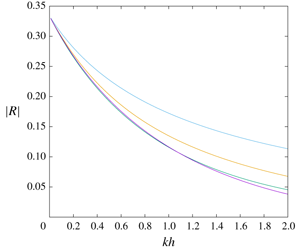
The Graphical Abstract represents graphs of the reflection coefficient by the Roseau bed profile for various model equations of the mild-slope type. Further details may be found in Porter (Reference Porter2019), the author of which provided the image.
Declaration of interests
The author reports no conflict of interest.
Appendix A
The variational principle
To derive (3.2) we begin with the Lagrangian density that represents kinetic energy minus the potential energy for the motion, constrained to satisfy the mass conservation condition  $\unicode[STIX]{x1D735}\boldsymbol{\cdot }\boldsymbol{q}=0$ within the fluid, namely
 $$\begin{eqnarray}L_{1}(\boldsymbol{q},\unicode[STIX]{x1D719},\unicode[STIX]{x1D702})=\int _{-h}^{0}\frac{1}{2}\unicode[STIX]{x1D70C}\boldsymbol{q}\boldsymbol{\cdot }\boldsymbol{q}\,\text{d}z-\left[\frac{1}{2}g\unicode[STIX]{x1D70C}\unicode[STIX]{x1D702}^{2}\right]_{z=0}+\int _{-h}^{0}\unicode[STIX]{x1D70C}\unicode[STIX]{x1D719}\unicode[STIX]{x1D735}\boldsymbol{\cdot }\boldsymbol{q}\,\text{d}z,\end{eqnarray}$$
the Lagrange multiplier  $\unicode[STIX]{x1D70C}\unicode[STIX]{x1D719}(x,y,z)$ being a new unknown function. For arbitrary variations
 $\unicode[STIX]{x1D6FF}\boldsymbol{q}=(\unicode[STIX]{x1D6FF}u,\unicode[STIX]{x1D6FF}v,\unicode[STIX]{x1D6FF}w)$,
 $\unicode[STIX]{x1D6FF}\unicode[STIX]{x1D719}$ and
 $\unicode[STIX]{x1D6FF}\unicode[STIX]{x1D702}$ we have
 $$\begin{eqnarray}\unicode[STIX]{x1D70C}^{-1}\unicode[STIX]{x1D6FF}L_{1}=\int _{-h}^{0}\left(\boldsymbol{q}\boldsymbol{\cdot }\unicode[STIX]{x1D6FF}\boldsymbol{q}+\unicode[STIX]{x1D6FF}\unicode[STIX]{x1D719}\unicode[STIX]{x1D735}\boldsymbol{\cdot }\boldsymbol{q}+\unicode[STIX]{x1D719}\unicode[STIX]{x1D735}\boldsymbol{\cdot }\unicode[STIX]{x1D6FF}\boldsymbol{q}\right)\,\text{d}z-[g\unicode[STIX]{x1D702}\unicode[STIX]{x1D6FF}\unicode[STIX]{x1D702}]_{z=0}.\end{eqnarray}$$
Following the substitution  $\unicode[STIX]{x1D719}\unicode[STIX]{x1D735}\boldsymbol{\cdot }\unicode[STIX]{x1D6FF}\boldsymbol{q}=\unicode[STIX]{x1D735}\boldsymbol{\cdot }\unicode[STIX]{x1D719}\unicode[STIX]{x1D6FF}\boldsymbol{q}-\unicode[STIX]{x1D6FF}\boldsymbol{q}\boldsymbol{\cdot }\unicode[STIX]{x1D735}\unicode[STIX]{x1D719}$, the
 $z$ component of the divergence can be integrated and the
 $x$ and
 $y$ components moved outside the integral to give
 $$\begin{eqnarray}\displaystyle & & \displaystyle \displaystyle \unicode[STIX]{x1D70C}^{-1}\unicode[STIX]{x1D6FF}L_{1}=\int _{-h}^{0}\left((\boldsymbol{q}-\unicode[STIX]{x1D735}\unicode[STIX]{x1D719})\boldsymbol{\cdot }\unicode[STIX]{x1D6FF}\boldsymbol{q}+\unicode[STIX]{x1D6FF}\unicode[STIX]{x1D719}\unicode[STIX]{x1D735}\boldsymbol{\cdot }\boldsymbol{q}\right)\text{d}z-[g\unicode[STIX]{x1D702}\unicode[STIX]{x1D6FF}\unicode[STIX]{x1D702}]_{z=0}+[\unicode[STIX]{x1D719}\unicode[STIX]{x1D6FF}w]_{z=0}-[\unicode[STIX]{x1D719}\unicode[STIX]{x1D6FF}w]_{z=-h}\nonumber\\ \displaystyle & & \displaystyle \qquad \displaystyle +\,\widetilde{\unicode[STIX]{x1D735}}\boldsymbol{\cdot }\int _{-h}^{0}\unicode[STIX]{x1D719}\unicode[STIX]{x1D6FF}\boldsymbol{q}\,\text{d}z-[\unicode[STIX]{x1D719}\unicode[STIX]{x1D6FF}\boldsymbol{q}\boldsymbol{\cdot }\widetilde{\unicode[STIX]{x1D735}}h]_{z=-h}.\end{eqnarray}$$
We now impose boundary conditions. First, the condition (2.4) representing zero mass flow across the bed requires the addition to  $L_{1}$ of
 $L_{2}=\unicode[STIX]{x1D70C}[\unicode[STIX]{x1D719}(w+\boldsymbol{q}\boldsymbol{\cdot }\widetilde{\unicode[STIX]{x1D735}}h)]_{z=-h}$ with
 $\unicode[STIX]{x1D6FF}L_{2}=\unicode[STIX]{x1D70C}[\unicode[STIX]{x1D6FF}\unicode[STIX]{x1D719}(w+\boldsymbol{q}\boldsymbol{\cdot }\widetilde{\unicode[STIX]{x1D735}}h)+\unicode[STIX]{x1D719}(\unicode[STIX]{x1D6FF}w+\unicode[STIX]{x1D6FF}\boldsymbol{q}\boldsymbol{\cdot }\widetilde{\unicode[STIX]{x1D735}}h)]_{z=-h}$, the choice
 $\unicode[STIX]{x1D719}(x,y,0)$ of the Lagrange multiplier used here being guided by the need to balance the term
 $-[\unicode[STIX]{x1D719}\unicode[STIX]{x1D6FF}w]_{z=-h}$ in (A 1). Finally, the inclusion of the remaining conditions, on
 $z=0$, is governed by the presence of
 $[\unicode[STIX]{x1D6FF}\unicode[STIX]{x1D702}]_{z=0}$ and
 $[\unicode[STIX]{x1D6FF}w]_{z=0}$ in (A 1), which implies the addition of
 $L_{3}=\unicode[STIX]{x1D708}[\unicode[STIX]{x1D70C}\unicode[STIX]{x1D702}w]_{z=0}$ to
 $L_{1}+L_{2}$, where
 $\unicode[STIX]{x1D708}$ is a constant to be determined.
Gathering the various contributions together we have
 $$\begin{eqnarray}\displaystyle & & \displaystyle \displaystyle \unicode[STIX]{x1D70C}^{-1}\unicode[STIX]{x1D6FF}(L_{1}+L_{2}+L_{3})=\int _{-h}^{0}\left((\boldsymbol{q}-\unicode[STIX]{x1D735}\unicode[STIX]{x1D719})\boldsymbol{\cdot }\unicode[STIX]{x1D6FF}\boldsymbol{q}+\unicode[STIX]{x1D6FF}\unicode[STIX]{x1D719}\unicode[STIX]{x1D735}\boldsymbol{\cdot }\boldsymbol{q}\right)\text{d}z-[(g\unicode[STIX]{x1D702}-\unicode[STIX]{x1D708}w)\unicode[STIX]{x1D6FF}\unicode[STIX]{x1D702}]_{z=0}\nonumber\\ \displaystyle & & \displaystyle \qquad \displaystyle +\,[(\unicode[STIX]{x1D719}+\unicode[STIX]{x1D708}\unicode[STIX]{x1D702})\unicode[STIX]{x1D6FF}w]_{z=0}-[(w+\boldsymbol{q}\boldsymbol{\cdot }\widetilde{\unicode[STIX]{x1D735}}h)\unicode[STIX]{x1D6FF}\unicode[STIX]{x1D719}]_{z=-h}+\widetilde{\unicode[STIX]{x1D735}}\boldsymbol{\cdot }\int _{-h}^{0}\unicode[STIX]{x1D719}\unicode[STIX]{x1D6FF}\boldsymbol{q}\,\text{d}z.\end{eqnarray}$$
Reference to (2.3) reveals that the choice  $\unicode[STIX]{x1D708}=-g/\text{i}\unicode[STIX]{x1D70E}$ ensures that
 $L=L_{1}+L_{2}+L_{3}$, which coincides with (3.2), has the required natural conditions. The expression (3.3) also follows by forming
 $\unicode[STIX]{x1D6FF}{\mathcal{L}}$ from (A 2) by means of (3.1) and invoking the divergence theorem to transfer the outstanding variation onto the lateral boundary.
The inner products
The evaluation of the coefficients in the MMSE (3.8) requires the following inner products. We use the abbreviation  $K=2kh$.
 $$\begin{eqnarray}\displaystyle & \displaystyle ||Z_{1}||^{2}=\text{sech}^{2}(kh)(K+\sinh K)/4k, & \displaystyle \nonumber\\ \displaystyle & \displaystyle \langle Z_{1},{\dot{Z}}_{1}\rangle =\text{sech}^{2}(kh)(\sinh K-K\cosh K)/4(K+\sinh K), & \displaystyle \nonumber\\ \displaystyle & \displaystyle ||{\dot{Z}}_{1}||^{2}=-k\,\text{sech}^{2}(kh)(K^{3}+3K^{2}\sinh K+6K-3\sinh 2K)/12(K+\sinh K)^{2}. & \displaystyle \nonumber\end{eqnarray}$$
These combine to give the coefficient  $v(h)$ in the concise MMSE (4.9) as
 $$\begin{eqnarray}v(h)=-\frac{K^{4}+4K^{3}\sinh K+3K^{2}(\cosh 2K+2)-3(2K+\sinh K)(\sinh 2K-\sinh K)}{3(\sinh K+K)^{4}}.\end{eqnarray}$$
The inner products associated with the CMSE that arise in § 4.3 are as follows.
 $$\begin{eqnarray}\displaystyle & \displaystyle a(h)=-\text{cosech}^{2}(kh)(\sinh K+K)/4k, & \displaystyle \nonumber\\ \displaystyle & \displaystyle b(h)=-\text{cosech}^{2}(kh)(\sinh K-K\cosh K)/4(K+\sinh K), & \displaystyle \nonumber\\ \displaystyle & \displaystyle c(h)=k\,\text{cosech}^{2}(kh)(K^{3}+3K^{2}\sinh K-6K+3\sinh 2K)/12(\sinh K+K)^{2}. & \displaystyle \nonumber\end{eqnarray}$$
It follows after some algebra that the coefficient  $\unicode[STIX]{x1D6FE}(h)\equiv f(kh)$ in the CMSE is given by
 $$\begin{eqnarray}\unicode[STIX]{x1D6FE}(h)=\frac{K^{4}+4K^{3}\sinh K+3K^{2}(\cosh 2K-2)-6K\sinh K+3\sinh K(\sinh K+\sinh 2K)}{3(\sinh K+K)^{4}},\end{eqnarray}$$
leading to the comparatively simple relationship
 $$\begin{eqnarray}v(h)+\unicode[STIX]{x1D6FE}(h)=2(\sinh 2K-2K)/(\sinh K+K)^{3}\end{eqnarray}$$
between the MMSE and the CMSE.
The new coefficients that arise in § 4.4 with  $Z_{3}=-z/h$ are as follows.
 $$\begin{eqnarray}b_{1}(h)=(1-kh\,\text{cosech}(kh))/k^{2}h,\quad c_{1}(h)=h/3\end{eqnarray}$$
and
 $$\begin{eqnarray}\unicode[STIX]{x1D6FE}_{1}(h)=\frac{4(12(\sinh (kh)-kh)^{2}+(kh)^{3}(\sinh K+K))}{3(kh)^{2}(\sinh K+K)}.\end{eqnarray}$$


