1 Context and objectives
In the context of large-eddy simulation (LES) of atmospheric flows over rough surfaces, better understanding of the multi-scale interchange between the canopy-driven dynamics and the large-scale dynamics of the surface layer could lead to more accurate and reliable wall models avoiding the computational expense of explicitly resolving the flow in the near-wall region. The nonlinear character of these canopy–atmosphere interactions calls specifically for a dynamic model of the interface, evolving with respect to the turbulent large-scale motions. Within this scope, the amplitude modulation approach developed for smooth-wall boundary layers represents an interesting prospect (Marusic, Mathis & Hutchins Reference Marusic, Mathis and Hutchins2010; Mathis, Hutchins & Marusic Reference Mathis, Hutchins and Marusic2011a ).
More than forty years ago Rao, Narasimha & Narayanan (Reference Rao, Narasimha and Narayanan1971), Brown & Thomas (Reference Brown and Thomas1977) and later Bandyopadhyay & Hussain (Reference Bandyopadhyay and Hussain1984) opened a new path to the modelling of turbulence in shear flows as they brought to light the phase relationship between large-scale events and the turbulent activity at smaller scales. Since then our understanding of turbulent boundary layers and coherent structure interplay has expanded significantly. The development of numerical simulations and particle image velocimetry (PIV) techniques have facilitated identifying coherent structures, notably by providing space-extended datasets. Near-wall turbulence is now known to consist of small-scale eddies generated at the wall, stretching and breaking down under the stress exerted by streaky large-scale motions, that emerge in the high-Reynolds-number boundary layers. One may notably refer to the works of Kim & Adrian (Reference Kim and Adrian1999), Adrian, Christensen & Liu (Reference Adrian, Christensen and Liu2000a
) or Hunt & Morrison (Reference Hunt and Morrison2000) for more detail on these aspects. In the last decade Marusic, Hutchins and their co-workers have regenerated the findings of Bandyopadhyay & Hussain (Reference Bandyopadhyay and Hussain1984) into a novel approach of the inter-scale interactions in turbulent boundary layers (Hutchins & Marusic Reference Hutchins and Marusic2007b
; Mathis, Hutchins & Marusic Reference Mathis, Hutchins and Marusic2009; Marusic et al.
Reference Marusic, Mathis and Hutchins2010; Talluru et al.
Reference Talluru, Baidya, Hutchins and Marusic2014). They demonstrated that small scales in the near-wall region can be described as being amplitude modulated by the large-scale fluctuations of momentum that prevail in the outer layer. This approach led to a predictive model put forward in Marusic et al. (Reference Marusic, Mathis and Hutchins2010) and Mathis et al. (Reference Mathis, Hutchins and Marusic2011a
) to reconstruct near-wall dynamics from a large-scale signal, measured much further from the wall. Frequency modulation was also revealed in Ganapathisubramani et al. (Reference Ganapathisubramani, Hutchins, Monty, Chung and Marusic2012) and Baars, Hutchins & Marusic (Reference Baars, Hutchins and Marusic2017) to occur in conjunction with amplitude modulation, although it was rather constrained to the inner part of the boundary layer. A similar approach was applied to a free jet by Fiscaletti, Ganapathisubramani & Elsinga (Reference Fiscaletti, Ganapathisubramani and Elsinga2015) who also observed modulations of the small scales. It is worth noting that the robustness and accuracy of this model rely on a clear separation in spectra between modulating and modulated signals (Mathis et al.
Reference Mathis, Hutchins and Marusic2009). Such a separation is obtained for high Reynolds numbers, at which the inner peak (fixed in wall units
 $\unicode[STIX]{x1D708}/U_{\unicode[STIX]{x1D70F}}$
, with
 $\unicode[STIX]{x1D708}$
the kinematic viscosity and
 $U_{\unicode[STIX]{x1D70F}}$
the friction velocity) and the outer peak (scaled with the boundary layer thickness
 $\unicode[STIX]{x1D6FF}$
) drift apart (Hutchins & Marusic Reference Hutchins and Marusic2007b
). This allows for a well-defined separation between the (modulating) large scales and the (modulated) small scales.
While the modulation approach has been extensively documented in the canonical smooth-wall case, its applicability to high-roughness cases like urban canopies remains to be rigorously characterised. High-roughness elements disrupt near-wall turbulence production by shedding intermediate-scale dynamics into the roughness sublayer, in particular in urban-type geometries. This perturbation could alter or prevent large-scale modulation. This also implies larger dissipative scales, hence reducing the spectral separation with large-scale motions (LSMs). As for the LSMs, they are not significantly different from the smooth-wall case: low/high momentum regions have been evidenced in many numerical simulations (e.g. Coceal et al.
Reference Coceal, Dobre, Thomas and Belcher2007; Lee, Sung & Krogstad Reference Lee, Sung and Krogstad2011; Inagaki et al.
Reference Inagaki, Castillo, Yamashita, Kanda and Takimoto2012). These LSMs actually leave a footprint deep within the roughness sublayer, despite the injection of intermediate scales by the roughness elements. This was confirmed experimentally by Mejia-Alvarez, Wu & Christensen (Reference Mejia-Alvarez, Wu and Christensen2014) dealing with a fully rough flow over an irregular roughness. Their analysis also alluded to the amplitude modulation (AM) by LSMs yet did not explore that aspect further. In fact, only a few studies have applied the amplitude modulation approach to high-roughness cases: Nadeem et al. (Reference Nadeem, Lee, Lee and Sung2015) performed direct numerical simulations (DNS) over a sparsely spaced rod-roughened wall and reported that rod-induced wakes strongly disrupted the amplitude modulation by the LSMs; Anderson (Reference Anderson2016) investigated the case of a staggered cubic canopy of plan density
 $\unicode[STIX]{x1D706}_{p}=25\,\%$
, similar to that of the present study but using LES of a channel flow. Amplitude modulation by LSMs was observed in the roughness sublayer and inside the canopy with a salient spatial variability. Note however the configuration presented a much lower ratio
 $\unicode[STIX]{x1D6FF}/h=4$
(where
 $h$
is the height of the roughness elements) that reduced greatly the gap between scales associated with LSMs and those associated with canopy-induced dynamics. To the authors’ knowledge, the only experimental investigation of AM in a highly roughened boundary layer was performed by Blackman & Perret (Reference Blackman and Perret2016) using wall-normal measurements.
The present work focuses on the spatial organisation of the modulation within the roughness sublayer. To that end, we make use of space-extended data acquired over a large region to gain access to nonlinear interactions over a wide range of length scales (§ 2). Spectral content analysis of the fluctuating kinetic energy is carried out in § 3 using spatially reconstructed velocity fields and temporal data, by means of Fourier and wavelet transforms. Since the outcome shows that high roughness reduces the separation with outer scales by injecting intermediate scales into the inner region of the flow, a diagnostic approach is put forward to choose the appropriate cutoff frequency used for scale decomposition (§ 4). This relies on third-order moments combining outer-layer large-scale fluctuations and small-scale kinetic energy terms in the roughness sublayer. This gives us access to the degree of amplitude modulation across all kinetic energy terms. Finally, § 5 brings new insights to the organisation in the wall-parallel plane of the amplitude modulations inside the roughness sublayer, and helps to complement the existing literature that generally focuses on the wall-normal evolution across the boundary layer (Mathis et al. Reference Mathis, Hutchins and Marusic2009; Ganapathisubramani et al. Reference Ganapathisubramani, Hutchins, Monty, Chung and Marusic2012; Baars et al. Reference Baars, Talluru, Hutchins and Marusic2015; Squire et al. Reference Squire, Baars, Hutchins and Marusic2016a ; Yao, Huang & Xu Reference Yao, Huang and Xu2018, etc.). Our analysis extends to all velocity components to give access to the kinetic energy, a Galilean invariant, hereby relating the amplitude modulation to coherent structures interplay around the large-scale motions.
2 Experiments
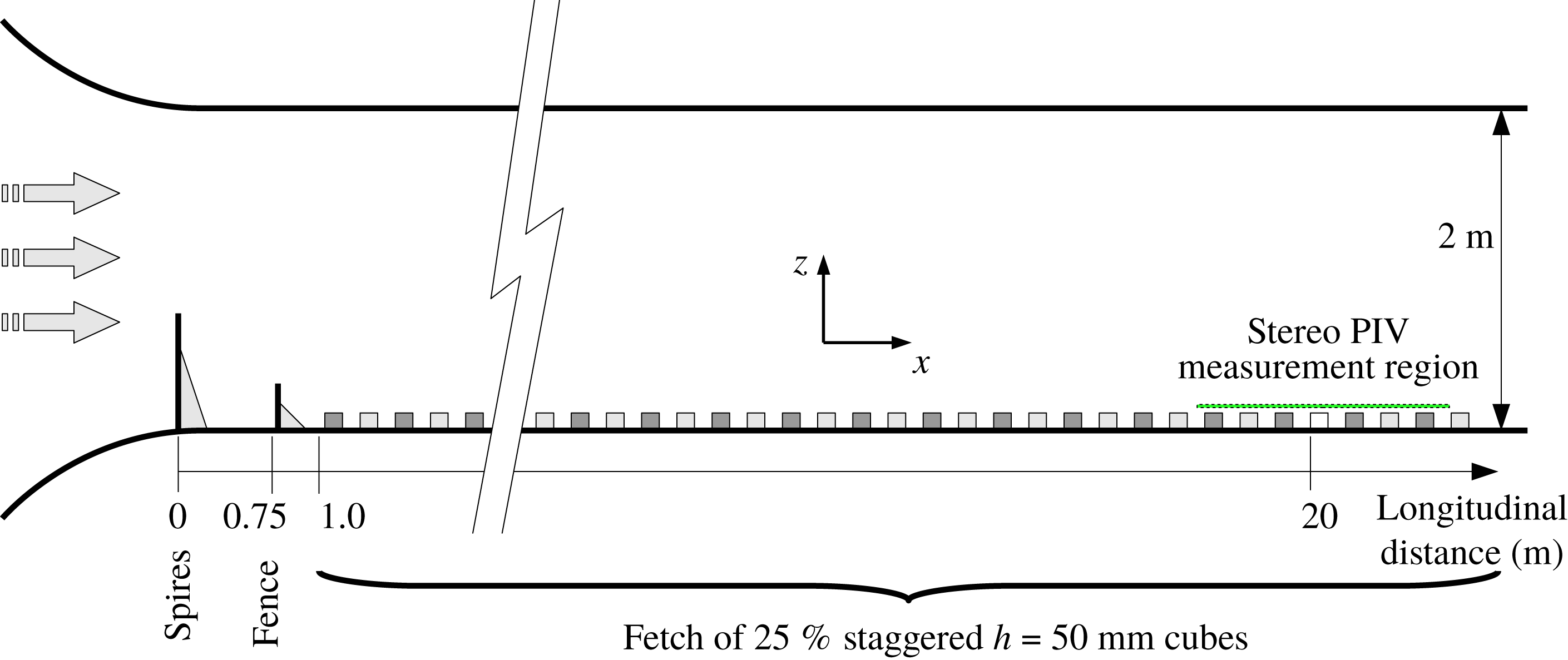
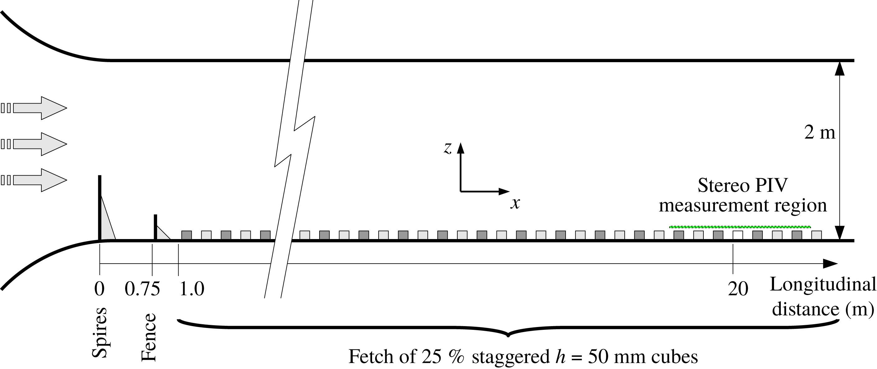
The lower part of a suburban-type atmospheric boundary layer was reproduced in the atmospheric boundary layer wind tunnel at the Laboratoire de recherche en Hydrodynamique, Energétique et Environnement Atmosphérique of Ecole Centrale de Nantes (LHEEA, Nantes, France), with a working section of dimensions
 $24~\text{m}\times 2~\text{m}\times 2~\text{m}$
(figure 1). The frame of reference
 $(\boldsymbol{e}_{x},\boldsymbol{e}_{y},\boldsymbol{e}_{z})$
, attached to the wind tunnel, corresponds to the streamwise, spanwise and wall-normal axes, respectively. The high-Reynolds-number turbulent boundary layer was tailored using five vertical tapered spires, 800 mm high and 134 mm wide at their base, in conjunction with a 200 mm-high solid fence, located 0.75 m downstream of the inlet across the working section. The flow then developed over an idealised urban-type roughness, consisting of a 22 m-long fetch of staggered
 $h=50~\text{mm}$
-high cubes, with a plan coverage
 $\unicode[STIX]{x1D706}_{p}=25\,\%$
. This urban canopy model constitutes a canonical geometry, known to present a wake-interference regime (Oke Reference Oke1988). Temperature was measured during acquisitions to estimate the kinematic viscosity and the pressure gradient along the test section,
 $(\unicode[STIX]{x1D708}/\unicode[STIX]{x1D70C}U_{e}^{3})(\text{d}P/\text{d}x)<-2.5\times 10^{-8}$
, which is small enough to have negligible impact on the boundary layer (DeGraaff & Eaton Reference DeGraaff and Eaton2000).
Sketch (not to scale) of the atmospheric wind tunnel at LHEEA laboratory, Nantes.
2.1 The atmospheric surface layer
Aerodynamic parameters of the atmospheric surface layer modelled here were deduced from form drag and streamwise velocity profiles
 $\langle U\rangle (z)$
(where
 $\langle \cdot \rangle$
denotes the time average,
 $U$
the instantaneous streamwise velocity and
 $u$
its fluctuation). Both displacement height
 $d$
and friction velocity
 $U_{\unicode[STIX]{x1D70F}}$
were estimated using wall-pressure measurements around a cube within the canopy (Perret et al.
Reference Perret, Piquet, Basley and Mathis2017, Reference Perret, Basley, Mathis and Piquet2018), as proposed by Cheng & Castro (Reference Cheng and Castro2002) and Cheng, Hayden & Robins (Reference Cheng, Hayden and Robins2007). Hot-wire measurements of streamwise velocity
 $U(z,t)$
were acquired across the boundary layer from
 $1.2h\leqslant z\leqslant 30h\sim 1.4\unicode[STIX]{x1D6FF}$
to identify roughness length
 $k_{0}$
from the logarithmic law
 $$\begin{eqnarray}\langle U\rangle ^{+}=\frac{\langle U\rangle }{U_{\unicode[STIX]{x1D70F}}}=\frac{1}{K}\ln \left(\frac{z-d}{k_{0}}\right)\end{eqnarray}$$
with the von Kármán constant
 $K$
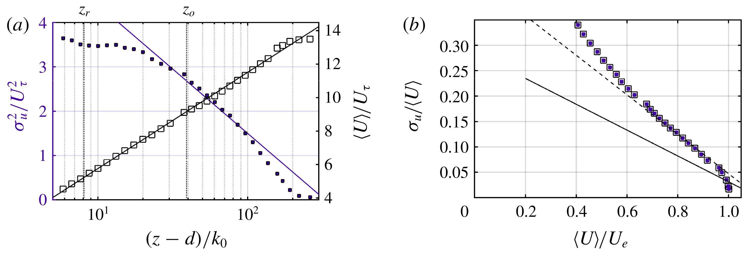
set to 0.4. Wall-normal profiles of mean and variance of streamwise velocity are plotted in figure 2(a), against the logarithmic law for the mean velocity given above in its meteorological form in (2.1), and the logarithmic law for the variance proposed by Marusic et al. (Reference Marusic, Monty, Hultmark and Smits2013)
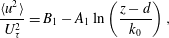 $$\begin{eqnarray}\frac{\langle u^{2}\rangle }{U_{\unicode[STIX]{x1D70F}}^{2}}=B_{1}-A_{1}\ln \left(\frac{z-d}{k_{0}}\right),\end{eqnarray}$$
where
 $B_{1}$
is a constant that depends on the flow geometry and wake parameter. Note that (2.1) and (2.2) assume the uniformity of the mean flow at a given wall distance
 $z$
but strictly speaking, that assumption is only valid outside the roughness sublayer. As for the mean velocity profile, it can be seen that a large portion of the profiles follows the logarithmic law, confirming the well-developed high-Reynolds-number character of the investigated flow. The influence of the spires can only be seen by the reduced strength of the wake component of the mean streamwise velocity profile. Regarding the variance profile, again, no deformation that could be attributed to the presence of spires upstream of the variance profile is visible. Close inspection of the power spectral density of the streamwise velocity component across the entire boundary layer (not shown here) confirmed the absence of any visible mark of the spires on the flow (Perret et al.
Reference Perret, Basley, Mathis and Piquet2018). Furthermore, it is remarkable that despite the completely different wall configuration in the present study, compared to the smooth-wall boundary layers examined by Marusic et al. (Reference Marusic, Monty, Hultmark and Smits2013), the value of the slope
 $A_{1}=1.26$
found in their study enables here a very good collapse of the data with the theoretical logarithmic profile originally proposed by Townsend for the streamwise variance (the value of the intercept
 $B_{1}$
has been adjusted as its value is expected to depend on the flow configuration). This confirms that in the region corresponding to the logarithmic portion of the variance profile, the structure of the flow is expected to match that of conventionally developing flows.
(a) Wall-normal profiles of mean streamwise velocity (black open squares) and standard deviation (purple filled squares), from hot-wire measurements presented in Perret et al. (Reference Perret, Piquet, Basley and Mathis2017, Reference Perret, Basley, Mathis and Piquet2018), plain lines depict logarithmic laws (2.1) and (2.2) and vertical dotted lines mark the wall-normal positions
 $z_{r}=1.5h$
and
 $z_{o}=5.0h$
(investigated in the following, as seen in figure 3). (b) Diagnostic plot as introduced in Castro, Segalini & Alfredsson (Reference Castro, Segalini and Alfredsson2013), the plain and dashed lines represent smooth (
 $a_{smooth}=0.286$
and
 $b_{smooth}=-0.255$
) and rough (
 $a_{rough}=0.436$
and
 $b_{rough}=-0.389$
) cases (2.3), respectively.
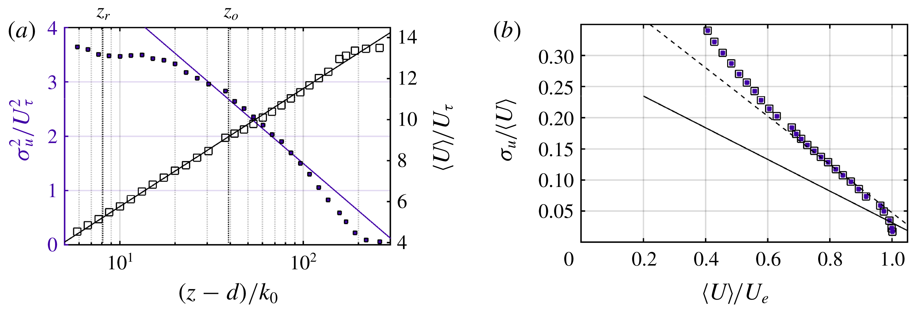
Figure 2(b) depicts the diagnostic plot introduced by Castro et al. (Reference Castro, Segalini and Alfredsson2013) to assess the self-similarity of rough-wall boundary layers and the fact that the flow is in fully rough regime and free of any potential spurious effects caused by the experimental set-up or the measurement method. This method consists in plotting the ratio of the standard deviation and the mean of the streamwise velocity component as a function of the mean streamwise velocity component normalised by the free-stream velocity
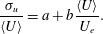 $$\begin{eqnarray}\frac{\unicode[STIX]{x1D70E}_{u}}{\langle U\rangle }=a+b\frac{\langle U\rangle }{U_{e}}.\end{eqnarray}$$
Based on an extensive survey of the literature, Castro et al. (Reference Castro, Segalini and Alfredsson2013) have shown that all the rough flow configurations collapse onto a single line in the outer region of the flow, resulting in a linear relationship between
 $\unicode[STIX]{x1D70E}_{u}/\langle U\rangle$
and
 $\langle U\rangle /U_{e}$
. The same was found for smooth-wall configurations but with a different slope. More recently, Placidi & Ganapathisubramani (Reference Placidi and Ganapathisubramani2017) have attributed the departure from the rough-wall asymptote to a possible lack of outer-layer similarity, which they tied to a too low ratio
 $\unicode[STIX]{x1D6FF}/h$
. Figure 2 right shows the present data in the form of the diagnostic plot along with the linear asymptote proposed by Castro et al. (Reference Castro, Segalini and Alfredsson2013) for the rough-wall (dashed line) and the smooth-wall (solid line) configurations. In the outer region, the collapse of the present data and the asymptote is excellent confirming that the flow is in fully rough regime and fully developed. Table 1 compiles the aerodynamic parameters of the canopy where,
 $\unicode[STIX]{x1D6FF}^{+}=U_{\unicode[STIX]{x1D70F}}\unicode[STIX]{x1D6FF}/\unicode[STIX]{x1D708}$
,
 $h^{+}=U_{\unicode[STIX]{x1D70F}}h/\unicode[STIX]{x1D708}$
and
 $\unicode[STIX]{x1D6FF}$
the boundary layer thickness measured where mean velocity reaches 99 % of the free-stream velocity
 $U_{e}$
. The aerodynamic parameters
 $k_{0}$
,
 $d$
and
 $U_{\unicode[STIX]{x1D70F}}$
are consistent with previous studies carried out over cubical canopies, both based on experiments (Cheng et al.
Reference Cheng, Hayden and Robins2007; Kanda et al.
Reference Kanda, Kanega, Kawai, Moriwaki and Sugawara2007; Hagishima et al.
Reference Hagishima, Tanimoto, Nagayama and Meno2009) and on numerical simulations (Kanda, Moriwaki & Kasamatsu Reference Kanda, Moriwaki and Kasamatsu2004; Leonardi & Castro Reference Leonardi and Castro2010; Ahn, Lee & Sung Reference Ahn, Lee and Sung2013). Note that in channel flows or some low-Reynolds-number simulations, the inertial region is drastically reduced, not unlike a developing boundary layer. This may lead to overestimated friction velocity
 $U_{\unicode[STIX]{x1D70F}}$
and thus underestimated roughness length
 $k_{0}$
(see for instance the dependency on
 $\unicode[STIX]{x1D6FF}/h$
reported in Cheng & Castro (Reference Cheng and Castro2002)). The present study considers a high-Reynolds-number boundary layer,
 $\unicode[STIX]{x1D6FF}/h\geqslant 20$
, and therefore comparison with lower
 $\unicode[STIX]{x1D6FF}/h$
configurations must be treated with caution. Discussing further the boundary layer profiles and aerodynamic parameters would be out of the scope of this study. This is done in more detail for different canopy configurations in other works by the authors (Blackman et al.
Reference Blackman, Perret, Calmet and Rivet2017; Perret et al.
Reference Perret, Piquet, Basley and Mathis2017, Reference Perret, Basley, Mathis and Piquet2018).
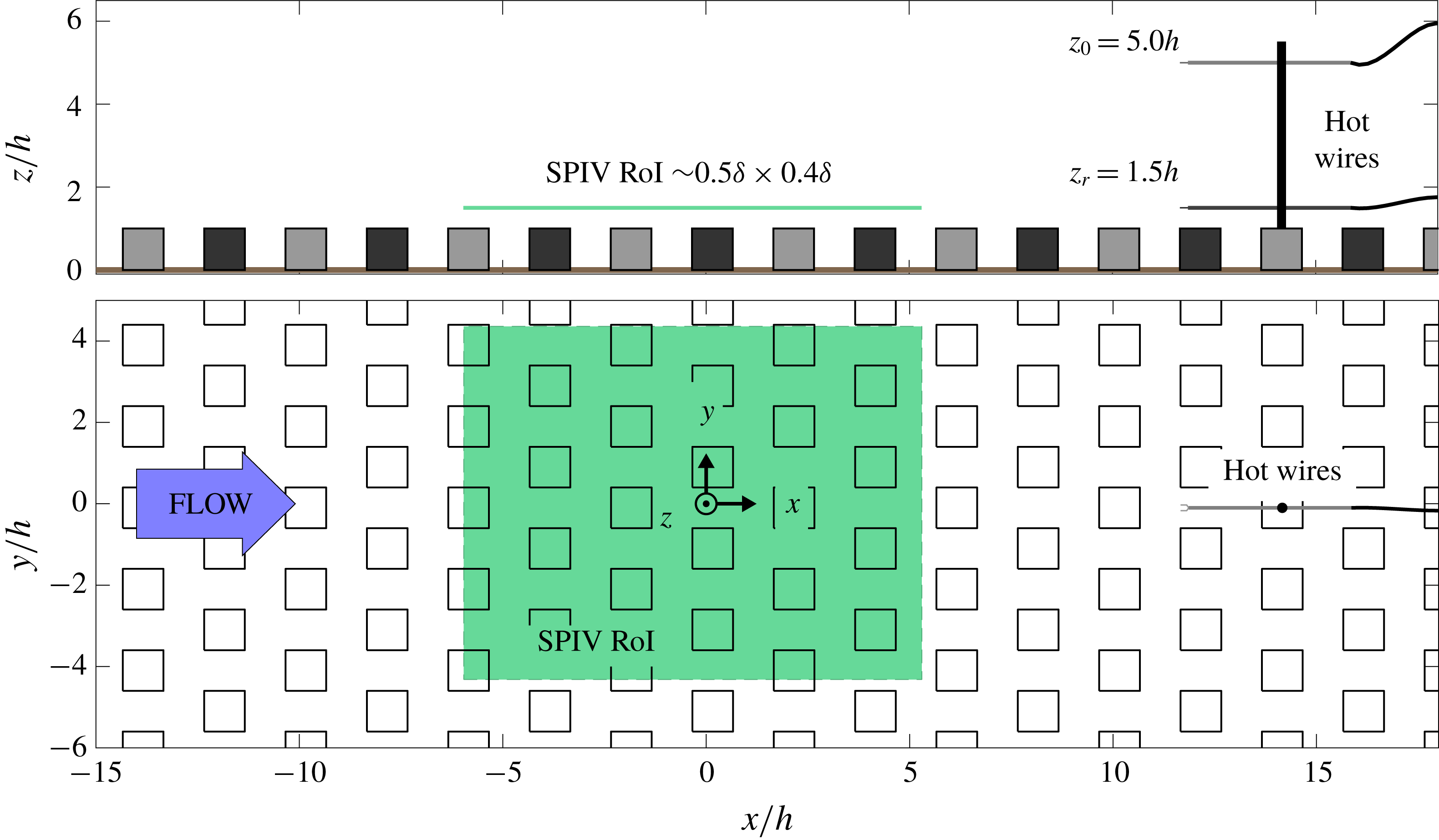
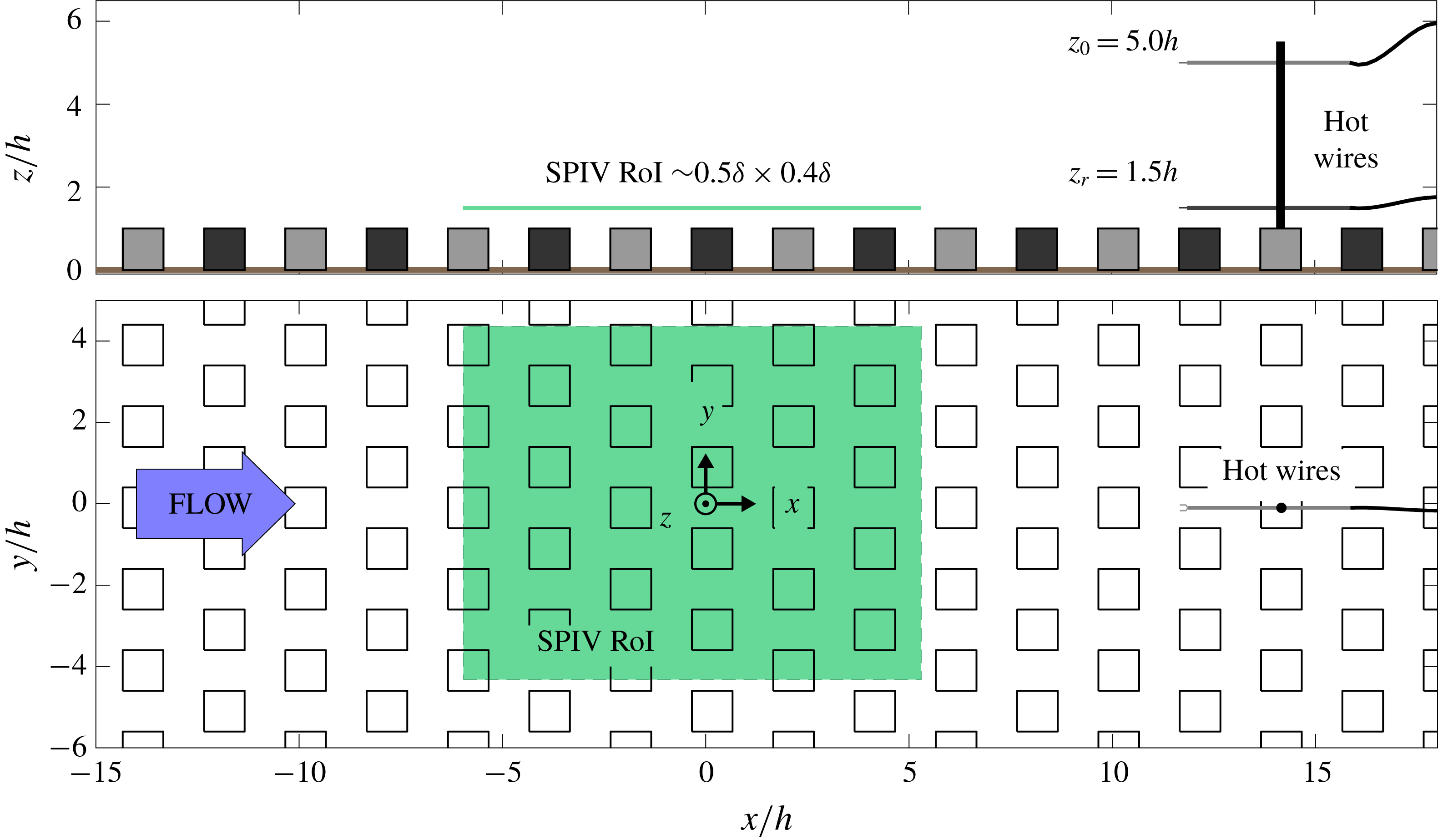
Sketch of the experimental set-up for stereoscopic PIV and hot-wire-synchronised measurements, side view (a) and top view (b). The shaded green area marks the region of interest of the stereoscopic PIV acquisitions.
Characteristics of the high-roughness canopy and the boundary layer.

2.2 Stereoscopic particle image velocimetry
Three-component two-dimensional stereoscopic particle image velocimetry (SPIV) measurements were conducted in a streamwise–spanwise plane at wall distance
 $z_{r}=1.5h$
in the roughness sublayer. Two
 $2048~\text{pixel}\times 2048~\text{pixel}$
cameras FlowSense were positioned at forward scattering angles
 $\unicode[STIX]{x1D6FC}=\{20^{\circ },53^{\circ }\}$
and associated with 60 mm and 105 mm Nikkor lenses at aperture
 $f_{\#}=2.8$
. The laser sheet was produced by a Nd–Yag laser (532 nm, 200 mJ/cavity); its thickness estimated between 3 and 5 mm.
It is worthwhile noting that such a high-Reynolds-number yet low-speed experiment (
 $\unicode[STIX]{x1D6FF}^{+}\simeq 3.2\times 10^{4}$
,
 $U_{e}\simeq 5.7~\text{m}~\text{s}^{-1}$
) imposes a region of interest (RoI) of large dimension to encompass the large-scale motions of the boundary layer as well as the obstacle-induced dynamics. The RoI extends over
 $11h\times 9h$
– that is,
 $0.5~\text{m}\times 0.45~\text{m}$
or
 $0.5\unicode[STIX]{x1D6FF}\times 0.4\unicode[STIX]{x1D6FF}$
– entailing a resolution of the velocity fields of about
 $20\times 12$
vectors/
 $h^{2}$
. The trade-off on the resolution of particle images impacts the attainable quality of SPIV fields, though only the smallest scales of the spectrum are significantly impacted. Image pre-processing was required (background cleaning, contrast enhancement and Gaussian filtering). Then cross-correlation and stereo reconstruction (polynomial) were performed using DANTEC Dynamic Studio software, which provides a
 $1/32$
th pixel resolution on the cross-correlation peak. Multi-pass computation was used from
 $64\times 64$
to
 $32\times 32$
pixel windows but no window deformation was required since no strong gradient occurs in such a wall-parallel plane. Up to 5 % outliers were detected in raw velocity fields prior to stereoscopic projection. Mainly located along the edges of the RoI, these outliers were replaced using a
 $3\times 3$
-window median filter. The rest of the random noise polluting the smallest scales of the flow was reduced using a low-pass
 $3\times 3$
-window Gaussian filter after stereoscopic reconstruction. The low-pass filtering effect is visible in power spectral densities presented in § 3.2 compared to hot-wire measurements. As for biased errors, mean velocity fields
 $(U,V,W)$
show a spatial heterogeneity up to
 $(0.022,0.022,0.0143)\,\overline{U}$
across the field – with
 $\overline{U}$
the averaged velocity. Standard deviations vary across the field by
 $(4\,\%,1\,\%,8\,\%)$
at most. These biases cumulate all sources of errors from SPIV projection bias and varying wall-normal distance of the laser sheet to background artefacts in particle images, such as reflections and laser sheet heterogeneities.
Five SPIV recordings were acquired at
 $f_{spiv}=7~\text{Hz}$
to form a dataset of
 $N_{s}=10\,500$
velocity fields designed to resolve both statistically and spatially the LSMs of the flow. Statistical convergence is assured with a total acquisition span comprising 8000 turnover time scales. At the same time, the streamwise extent of the vector fields is such that the corresponding convective time of the large-scale events (using Taylor’s hypothesis) is lower than the interval time step between two consecutive snapshots, i.e.
 $1/f_{spiv}\lesssim \unicode[STIX]{x1D6FF}/U_{e}$
. This allows us to stitch together successive snapshots, whose content captures all the dynamics of the large-scale motions, as detailed in § 3.
2.3 Hot-wire anemometry
Streamwise velocity measurements were obtained by constant-temperature hot-wire anemometry (HWA) using
 $5~\unicode[STIX]{x03BC}\text{m}$
-diameter 1.25 mm-long probes DANTEC-55P11 and DISA anemometers associated with anti-aliasing linear-phase elliptic filters. HWA time series were synchronised with SPIV acquisitions and span over a total duration of
 $T_{HWA}=5\times 20~\text{min}$
(
 $T_{HWA}U_{e}/\unicode[STIX]{x1D6FF}>3\times 10^{4}$
). Two probes were used downstream of the SPIV region of interest (see figure 3), located at a distance
 $h$
downstream of a cube. The first probe was aligned with the SPIV plane at
 $z_{r}=1.5h$
to support SPIV data through Taylor’s hypothesis while the second one was set at
 $z_{o}=5.0h$
to give access to cross-correlation with outer-layer dynamics. It should be noted that this experimental set-up allows capture of the spatial heterogeneity of the flow close to the canopy (PIV), and gives access to one-point time-series information (HWA) from outside the roughness sublayer, where the flow is spatially homogeneous on average and insensitive to the heterogeneity caused by the high-roughness elements (see Appendix for details).
The choice of these wall-normal distances has been driven by several considerations. On one hand,
 $z_{r}=1.5h$
is a location close to the top of the canopy, where the exchanges between the boundary layer and the canopy take place. Blackman & Perret (Reference Blackman and Perret2016) have shown that
 $z_{r}=1.5h$
corresponds approximately to the maximum of the term
 $\widetilde{u}u^{\prime 2}$
, where
 $\widetilde{u}$
and
 $u^{\prime }$
are the large-scale and small-scale contributions to fluctuations of streamwise velocity, respectively. It is also worth noting that the three-dimensional effects caused by the cubes alter the reliability of HWA measurements when getting closer to the canopy. On the other hand,
 $z_{o}=5.0h$
has been chosen so as to have a reference point within the outer layer, hypothesised to be out of the influence of the cubes. Several studies have been performed in a similar cube array configuration (Cheng & Castro Reference Cheng and Castro2002; Rivet Reference Rivet2014), who found that for a packing density of 25 % the upper limit of the roughness sublayer, defined as the height at which the spatial variation of the Reynolds shear stress falls below 5 %, is approximately
 $1.8$
to
 $1.85h$
. In the present study,
 $z_{o}=5.0h$
is well above this limit and the spatial variation of the shear stress remains below 2 % (while it reaches 9 % at
 $z_{r}=1.5h$
).
3 Datasets and spectral content
This section presents the combined results of SPIV and synchronised HWA data at both
 $z_{r}=1.5h$
and
 $z_{o}=5.0h$
, focusing on the spectral signature of the flow dynamics depending on the wall-normal location and the velocity component under study.
3.1 Taylor’s hypothesis to reconstruct large-scale motions
Each velocity field
 $\{\boldsymbol{U}(x,y,z_{r})\}$
out of the SPIV wall-parallel plane at
 $z_{r}=1.5h$
is decomposed as
 $$\begin{eqnarray}\boldsymbol{U}(x,y,z_{r})=\langle \boldsymbol{U}\rangle +\boldsymbol{u}=(\langle U\rangle ,\langle V\rangle ,\langle W\rangle )+(u,v,w),\end{eqnarray}$$
where
 $\langle \cdot \rangle$
denotes the time average and
 $\boldsymbol{u}(x,y,z_{r},t)$
is the fluctuating field at instant
 $t$
. The fluctuating time series
 $u_{r}(t)$
is decomposed the same way from HWA data recorded at the same wall-normal location
 $z_{r}=1.5h$
. The flow is in a steady regime and the spatial heterogeneity induced by the canopy is already low at
 $z_{r}$
: it has been assessed through statistical moments and found to be generally less than 2 %. Keeping that in mind, the approximation of frozen turbulence (Taylor Reference Taylor1938) is applied to reconstruct streamwise information with successive SPIV fields and compare the resulting signal to HWA time series. In practice this entails assuming the existence of a scale-independent advection velocity
 $U_{a}$
such that
 $$\begin{eqnarray}\unicode[STIX]{x1D702}(x,z,t)\equiv x-x_{0}-tU_{a}(z),\quad t_{\unicode[STIX]{x1D702}}(x,z,t)\equiv t-(x-x_{0})/U_{a}(z)\end{eqnarray}$$
are defined as the new abscissa and time coordinate, respectively, with
 $x_{0}$
the origin in the SPIV field. Space–time correlation between SPIV streamwise series
 $u_{r}(x,y_{hw},t)$
and HWA time series
 $u_{r}(x_{hw},y_{hw},t)$
gives the estimation
 $U_{a}(z_{r})=6.7U_{\unicode[STIX]{x1D70F}}$
, which matches the profile reported in Castro, Cheng & Reynolds (Reference Castro, Cheng and Reynolds2006). A two-dimensional fluctuating field
 $\boldsymbol{u}_{r}(\unicode[STIX]{x1D702},y)$
can then be built by concatenation of SPIV snapshots, whose large extension
 $L_{x}=0.55\unicode[STIX]{x1D6FF}>U_{a}/f_{spiv}$
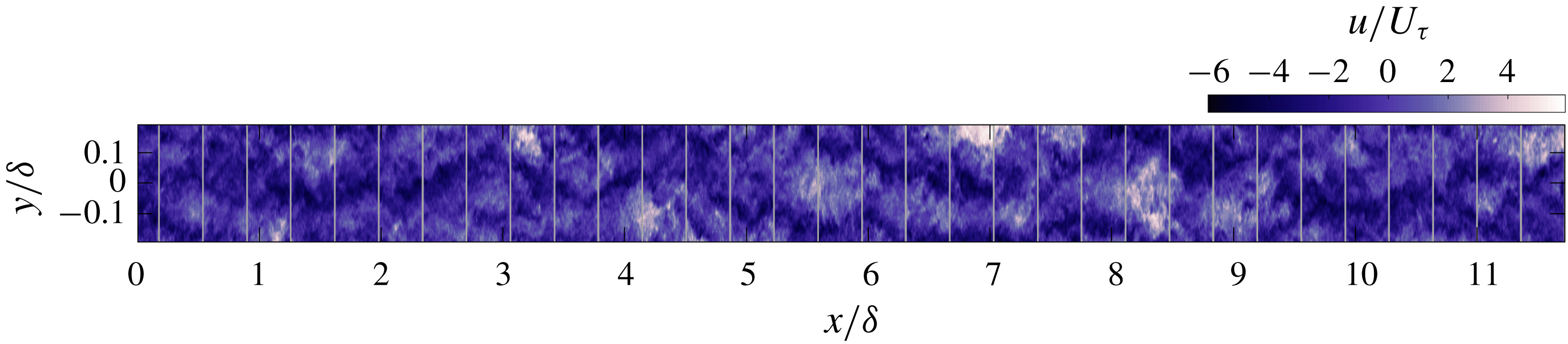
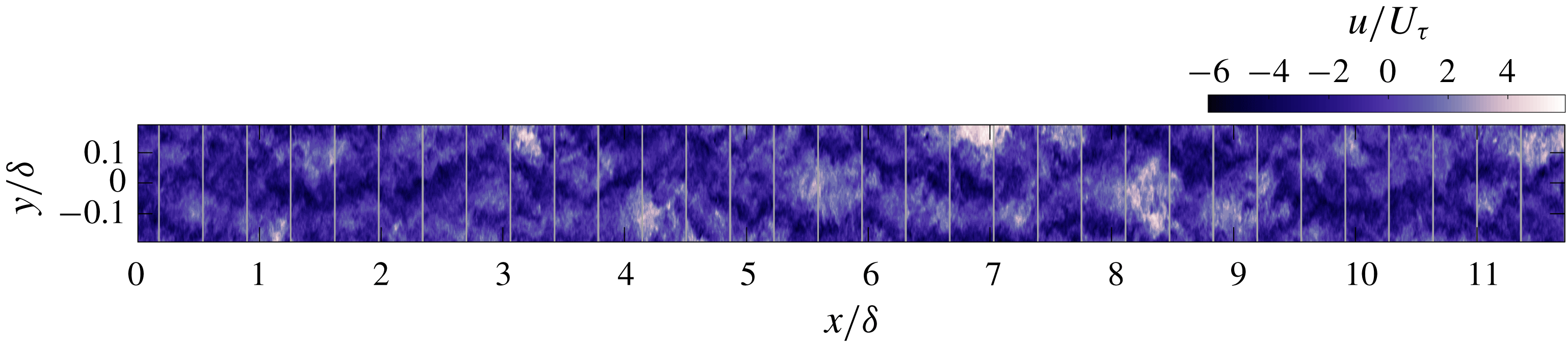
provides a conservative overlap. A sample of stitched velocity field is given in figure 4, showing a qualitatively good recombination and continuity between the stitched snapshots. Particularly, large-scale motions of elongated regions in the streamwise direction with a slightly spanwise meandering effect are clearly observed as in the smooth turbulent boundary layer (Hutchins & Marusic Reference Hutchins and Marusic2007a
).
Excerpt of stitched velocity field in plane
 $z_{r}=1.5h$
, with contours of fluctuations of streamwise velocity
 $u$
, normalised by friction velocity
 $U_{\unicode[STIX]{x1D70F}}$
. Vertical lines mark the junctions between SPIV fields.
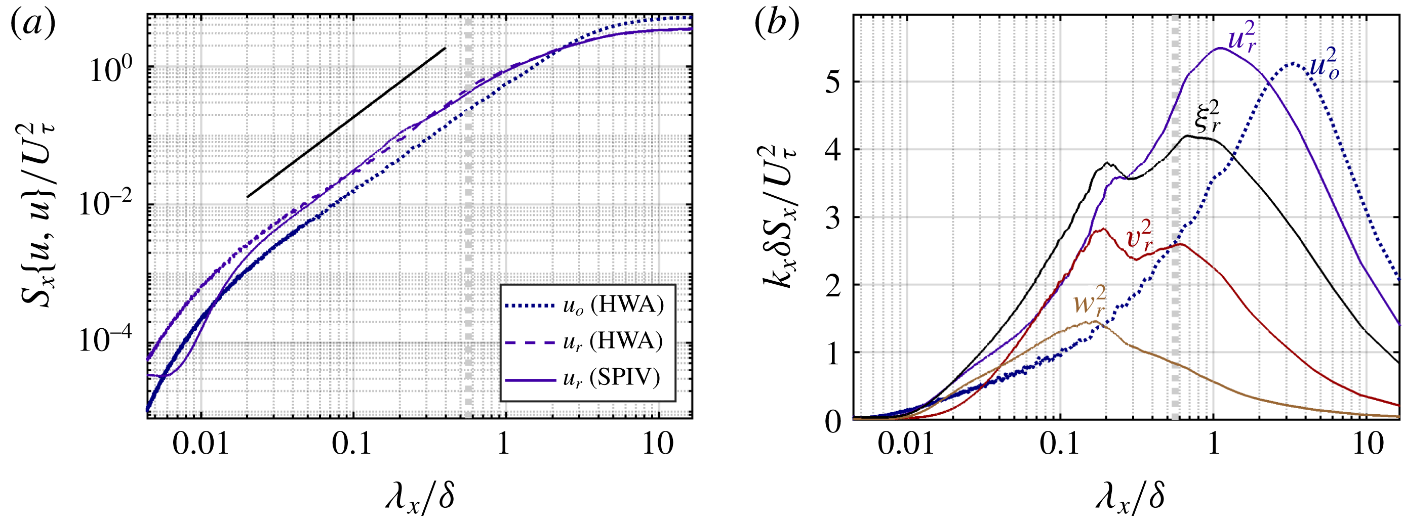
The streamwise auto-spectrum
 $S_{x}\{u_{r},u_{r}\}$
of the resulting field is compared with that of HWA data
 $u_{r}(\unicode[STIX]{x1D702}(x_{hw},z_{r},t))$
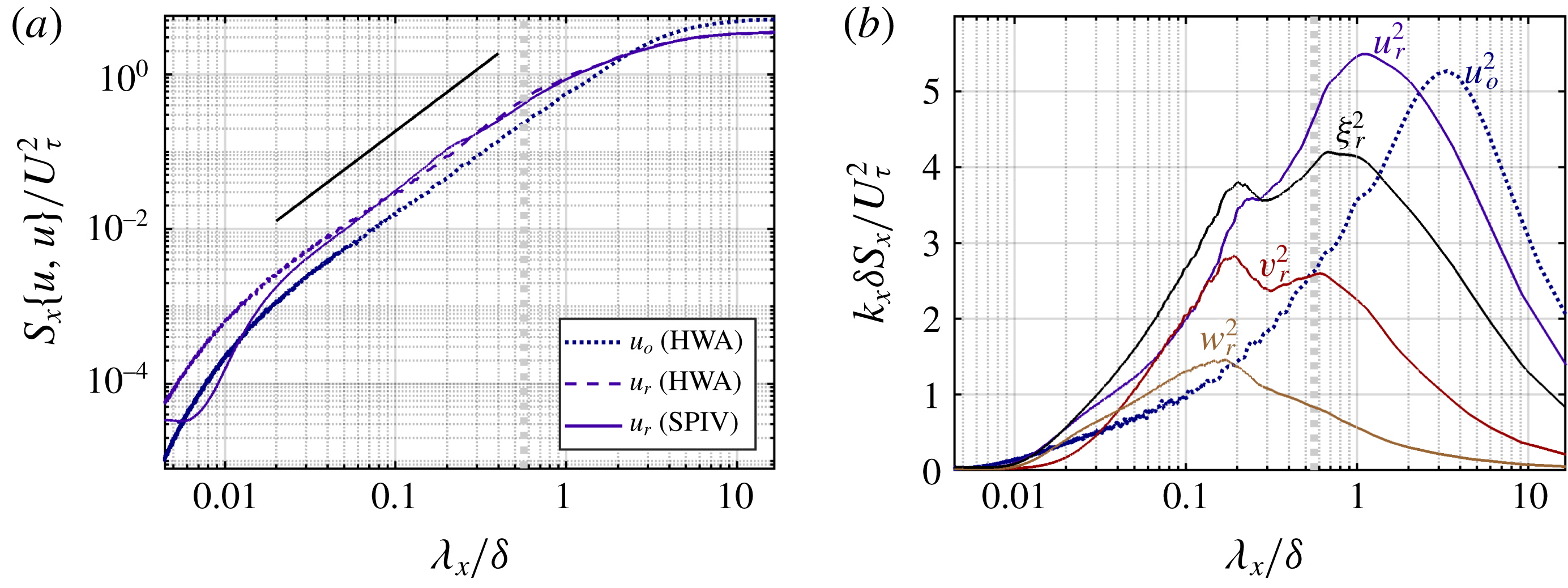
in figure 5(a). The two match fairly well in the large-scale range that is hence properly reconstructed using Taylor’s approximation. On the other hand, there exist discrepancies around
 $\unicode[STIX]{x1D706}_{x}\simeq 0.2\unicode[STIX]{x1D6FF}\sim 4h$
, which derive from spatial heterogeneity caused by the roughness elements. This infringement to Taylor’s hypothesis remains limited to scales associated with the canopy pattern. This is visible in SPIV pre-multiplied spectra plotted in figure 5(b), where a secondary peak can be observed at
 $\unicode[STIX]{x1D706}_{x}\simeq 0.2\unicode[STIX]{x1D6FF}$
(
 $\simeq 4h$
). This does not impede the reconstruction, which involves much larger scales such that
 $L_{x}>U_{a}/f_{spiv}\sim 0.4\unicode[STIX]{x1D6FF}$
.
3.2 Energy streamwise spectrum
The different contributions of fluctuating kinetic energy
 $\unicode[STIX]{x1D709}_{r}^{2}$
to the streamwise energy spectrum
 $\unicode[STIX]{x1D6EF}_{r}$
in plane
 $z_{r}=1.5h$
 $$\begin{eqnarray}\unicode[STIX]{x1D709}_{r}^{2}={\textstyle \frac{1}{2}}(u_{r}^{2}+v_{r}^{2}+w_{r}^{2}),\quad \unicode[STIX]{x1D6EF}_{r}(\unicode[STIX]{x1D706}_{x})={\textstyle \frac{1}{2}}(S_{x}\{u_{r},u_{r}\}+S_{x}\{v_{r},v_{r}\}+S_{x}\{w_{r},w_{r}\}),\end{eqnarray}$$
are presented in figure 5(b) where they are compared to that of
 $u_{o}(\unicode[STIX]{x1D702}(x_{hw},z_{o},t))$
, which assumes
 $U_{a}(z_{o})\simeq \langle U\rangle (z_{o})=9.5U_{\unicode[STIX]{x1D70F}}$
(Castro et al.
Reference Castro, Cheng and Reynolds2006). Streamwise velocity fluctuations exhibit a peak at large scales, centred on
 $\unicode[STIX]{x1D706}_{x}\sim \unicode[STIX]{x1D6FF}$
in the roughness sublayer and attaining
 $\unicode[STIX]{x1D706}_{x}\simeq 3\unicode[STIX]{x1D6FF}$
to
 $4\unicode[STIX]{x1D6FF}$
in the outer layer. These
 $\unicode[STIX]{x1D6FF}$
-scaled LSMs are typical of wall-bounded flows (Blackwelder & Kovasznay Reference Blackwelder and Kovasznay1972; Kim & Adrian Reference Kim and Adrian1999; Ganapathisubramani et al.
Reference Ganapathisubramani, Hutchins, Hambleton, Longmire and Marusic2005; McKeon Reference McKeon2017), identified as elongated meandering regions of alternative low and high momentum encompassing the whole boundary layer thickness. As already shown by Squire et al. (Reference Squire, Morill-Winter, Hutchins, Schultz, Klewicki and Marusic2016b
) for weakly roughened wall, we find again here that the large-scale log-region events remain independent of the rough characteristic of the wall even in the case of high-roughness elements. On the other hand, it should then be emphasised that the inner layer, as encountered in smooth or weakly roughened wall boundary layers, is largely altered here by the high-roughness elements and replaced by the canopy and roughness sublayers. Therefore the wall-normal position
 $z_{r}$
is in the near-canopy region and remains far from the outer region. Contrarily to smooth or weakly roughened walls (Hutchins & Marusic Reference Hutchins and Marusic2007b
; Monty et al.
Reference Monty, Hutchins, Marusic and Chong2009), the high roughness of the canopy removes the inner peak and sheds wake-type dynamics at intermediate scales, as seen in figure 5(b) by the secondary peak appearing at
 $\unicode[STIX]{x1D706}_{x}\simeq 0.2\unicode[STIX]{x1D6FF}$
(
 $\simeq 4h$
). This peak, characterising the signature of canopy-induced dynamics, appears more strikingly in wall-normal and spanwise velocity spectra and is confined to the roughness sublayer (Basley & Perret Reference Basley and Perret2017). It should be noted that the gap between this new small-scale range and outer scaling motions is now constrained by the ratio
 $\unicode[STIX]{x1D6FF}/h$
rather than
 $\unicode[STIX]{x1D6FF}^{+}$
, even for high Reynolds numbers.
Streamwise spectra from HWA and SPIV data are compared using Taylor’s hypothesis: (a) auto-spectra of streamwise velocity at both
 $z_{r}=1.5h$
and
 $z_{o}=5.0h$
, (b) pre-multiplied spectra associated with
 $u_{o}^{2}$
and the terms of
 $\unicode[STIX]{x1D709}_{r}^{2}=(u_{r}^{2}+v_{r}^{2}+w_{r}^{2})/2$
. Power spectral densities (PSDs) are estimated over 1500, 50 %-overlapped 2s-long windows. The grey dotted line indicates the streamwise extent of the SPIV field of view and the black slope the
 $5/3$
power law.
3.3 Time–frequency analysis using wavelet transforms
Spectral analysis can be extended to joint time–frequency description of the flow dynamics to help track the occurrence of inter-scale modulations. To give access to the time evolution of the spectral signature of the flow, continuous wavelet transforms (Burrus, Gopinath & Guo Reference Burrus, Gopinath and Guo1998) are performed on the combined fluctuating fields
 $\{u_{r},v_{r},w_{r}\}$
. Wavelet analysis relies on projecting the dynamics onto a base of similar functions generated from a single characteristic shape, often referred to as mother wavelet. This wavelet is defined as a function of (dimensionless) time
 $t/s$
, where
 $s$
is the characteristic scale. Frequency decomposition is then achieved by applying the mother wavelet onto a selected set of scales. Contrary to harmonic functions used in Fourier transform, wavelet functions have a finite extension that produces a time-dependent coefficient of projection. As a result, one obtains an instantaneous spectral information of the dynamics. It must be noted that using non-periodic functions also implies a non-unique frequency signature: wavelet functions are typically defined as a wave packet, associated with a broad peak about a central frequency. Similarly, time resolution depends directly on the scale over which the wavelet spans.
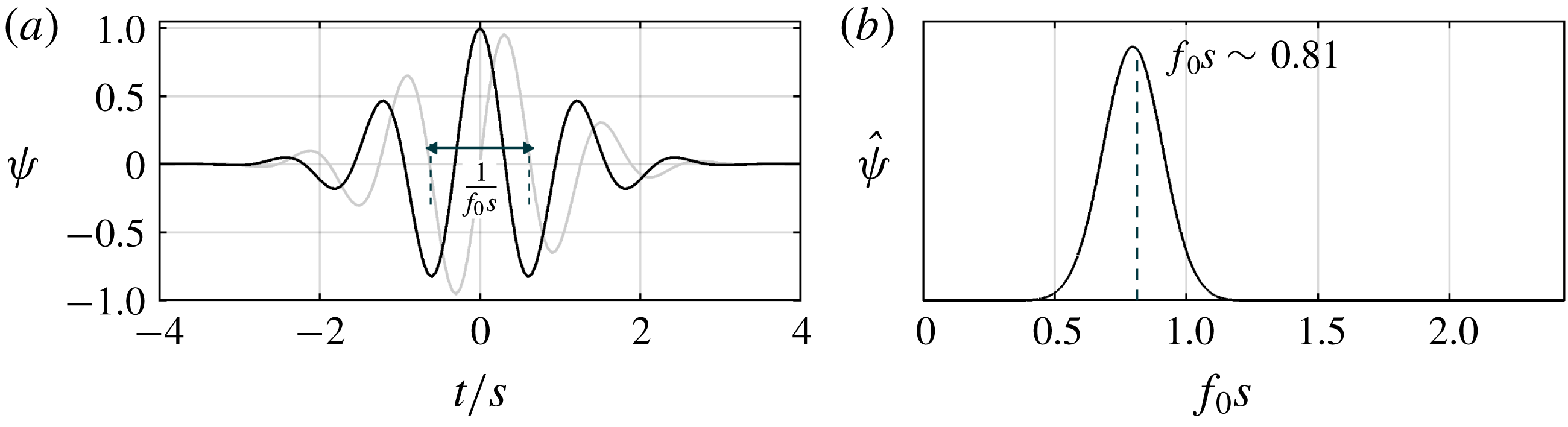
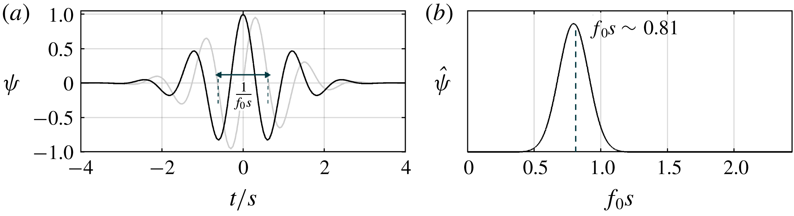
The forthcoming analysis uses the (analytic) Morlet wavelet, which consists in a complex harmonic wave localised with a Gaussian-shaped envelope (figure 6 a). It writes
 $$\begin{eqnarray}\unicode[STIX]{x1D713}(t/s)=\text{e}^{\text{i}\unicode[STIX]{x1D714}t/s}\text{e}^{-(|t/s|^{2})/2},\end{eqnarray}$$
where
 $s$
denotes the scale under consideration and
 $\unicode[STIX]{x1D714}$
is the non-dimensional angular frequency. The equivalent frequency to scale
 $s$
is the central frequency
 $f_{0}=0.8125/s$
of the peak in the spectral space (figure 6
b). In their study of amplitude and frequency modulations of small-scale dynamics Baars et al. (Reference Baars, Talluru, Hutchins and Marusic2015) compared the use of Morlet (3.4) and Mexican hat wavelets. The harmonic nature of Morlet wavelet offers a better frequency resolution while Mexican hat presents a shorter support time and is therefore more precise time wise. Ultimately, both functions produced similar results in Baars et al. (Reference Baars, Talluru, Hutchins and Marusic2015), except for discrepancies in the estimation of modulation time shifts. The present analysis aims for a trade-off by using Morlet wavelet with a reduced angular frequency
 $\unicode[STIX]{x1D714}=5$
compared to that chosen by Baars et al. (Reference Baars, Talluru, Hutchins and Marusic2015) (
 $\unicode[STIX]{x1D714}=6$
therein).
Analytic Morlet wavelet normalised by scale
 $s$
with angular frequency
 $\unicode[STIX]{x1D714}=5$
. Real (black) and imaginary (grey) parts are plotted in physical space in (a). Corresponding one-sided spectrum is shown in (b), with associated central frequency
 $f_{0}=0.8125/s$
.
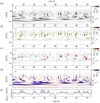
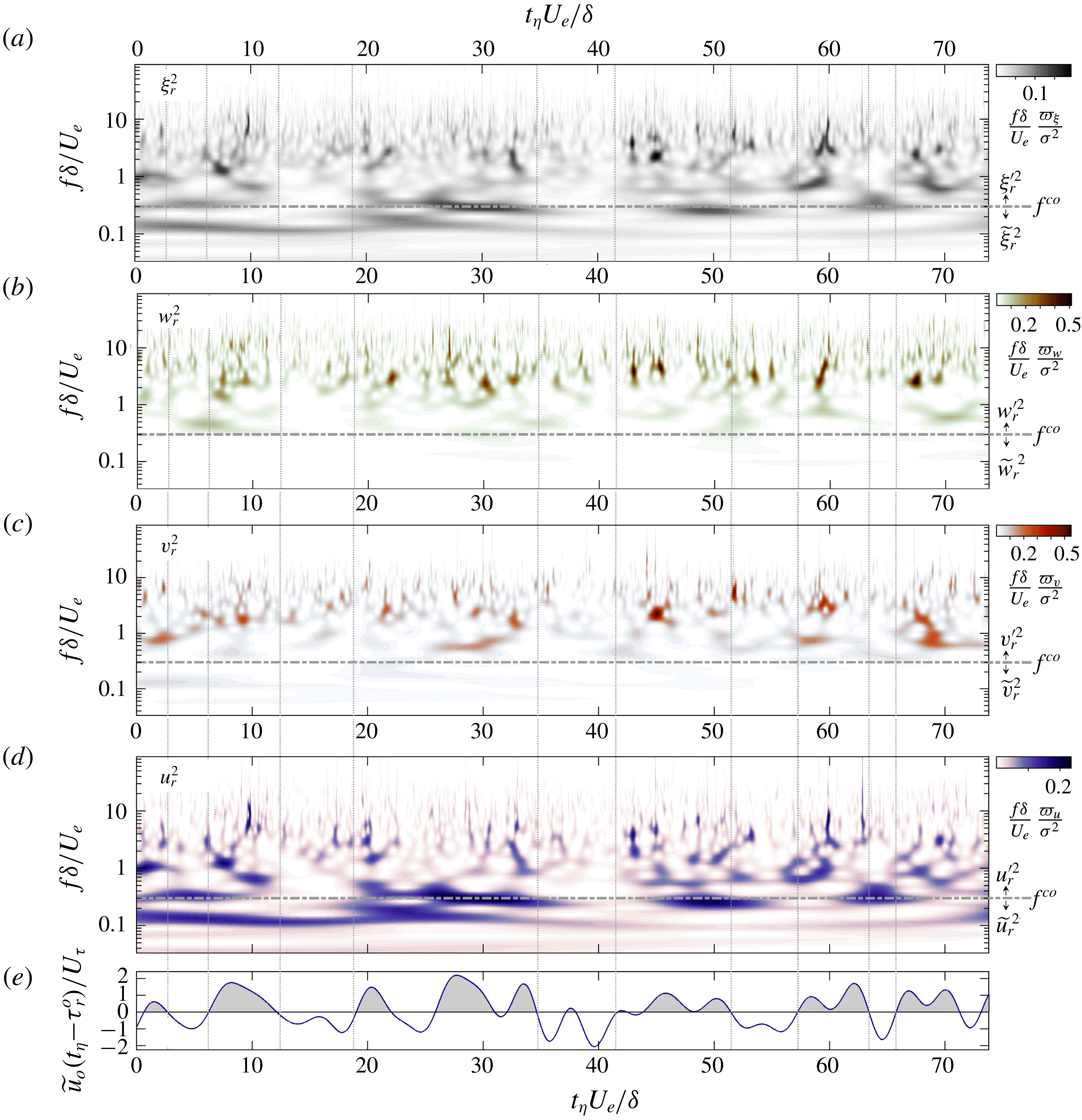
Pre-multiplied wavelet power spectrum (using Morlet wavelet) applied to streamwise time series
 $(t_{\unicode[STIX]{x1D702}},y_{hw},z_{r})$
extracted from SPIV data: from top to bottom, (a)
 $\unicode[STIX]{x1D71B}_{\unicode[STIX]{x1D709}^{2}}(t_{\unicode[STIX]{x1D702}},f)$
, (b)
 $\unicode[STIX]{x1D71B}_{w}(t_{\unicode[STIX]{x1D702}},f)$
, (c)
 $\unicode[STIX]{x1D71B}_{v}(t_{\unicode[STIX]{x1D702}},f)$
and (d)
 $\unicode[STIX]{x1D71B}_{u}(t_{\unicode[STIX]{x1D702}},f)$
. In each graph the horizontal dashed grey line marks cutoff frequency
 $f^{co}=0.3\,U_{e}/\unicode[STIX]{x1D6FF}$
(discussed in § 4.2 and used thereafter). Outer-layer large-scale fluctuations
 $\widetilde{u_{o}}$
(see § 4.2) are reported in (e) for reference, taking into account the time shift
 $\unicode[STIX]{x1D70F}_{r}^{o}=-0.80\unicode[STIX]{x1D6FF}/U_{e}$
between
 $u_{o}$
and
 $u_{r}$
signals (see § 4.1).
For a given scale
 $s$
, the wavelet coefficient
 $\breve{X}(t,s)$
of a signal
 $X(t)$
is obtained by convoluting the target signal with the wavelet function
 $\unicode[STIX]{x1D713}(t/s)$
 $$\begin{eqnarray}\breve{X}(t,s)=\int X(t^{\prime })\unicode[STIX]{x1D713}^{\ast }\left(\frac{t-t^{\prime }}{s}\right)\,\text{d}t^{\prime },\end{eqnarray}$$
where
 $(\cdot )^{\ast }$
is the complex conjugate. Note that in practice convolution is performed in spectral space through Fourier transforms. Target signals are here extracted from SPIV data at
 $z_{r}=1.5h$
, namely
 $X(t)=\{u_{r}(t_{\unicode[STIX]{x1D702}},y_{hw}),v_{r}(t_{\unicode[STIX]{x1D702}},y_{hw}),w_{r}(t_{\unicode[STIX]{x1D702}},y_{hw})\}$
, and wavelet transforms are computed over a set of logarithmically distributed scales corresponding to central frequencies ranging from
 $0.033\leqslant f_{0}\unicode[STIX]{x1D6FF}/U_{e}\leqslant 89$
. The wavelet power spectrum is computed from the squared modulus of wavelet coefficients normalised by the scale
 $s$
 $$\begin{eqnarray}\unicode[STIX]{x1D71B}_{X}(t_{\unicode[STIX]{x1D702}},f_{0})=\frac{|\breve{X}(t_{\unicode[STIX]{x1D702}},s)|^{2}}{s}.\end{eqnarray}$$
Similarly to (3.3), the wavelet spectrum corresponding to total kinetic energy is defined as
 $$\begin{eqnarray}\unicode[STIX]{x1D71B}_{\unicode[STIX]{x1D709}}(t_{\unicode[STIX]{x1D702}},f)={\textstyle \frac{1}{2}}(\unicode[STIX]{x1D71B}_{u}+\unicode[STIX]{x1D71B}_{v}+\unicode[STIX]{x1D71B}_{w}).\end{eqnarray}$$
Excerpts of pre-multiplied wavelet spectra are plotted for all terms of kinetic energy in figure 7. With wavelet transforms, the spectral contents of the flow unfold to reveal the differences between velocity components even more strikingly than in Fourier spectra. Large-scale motions are seen exclusively in the spectrum of streamwise component,
 $\unicode[STIX]{x1D71B}_{u}$
, while spectra
 $\unicode[STIX]{x1D71B}_{v}$
and
 $\unicode[STIX]{x1D71B}_{w}$
are contained in the small-scale range. A cutoff frequency could indeed be chosen to separate the dynamics of both
 $v$
and
 $w$
components from the large-scale fluctuations of streamwise velocity. That aspect is discussed in depth in § 4.2.
Furthermore, time–frequency plots displayed in figure 7 clearly illustrate the amplitude modulation of small-scale dynamics by large-scale streamwise velocity in the outer layer. Note that
 $\widetilde{u_{o}}$
is low-pass filtered from hot-wire measurements at
 $z_{o}=5.0h$
, as detailed later in § 4.2. To negative fluctuations of
 $\widetilde{u_{o}}$
correspond a reduced energy of the small-scale content in all components, while positive fluctuations of
 $\widetilde{u_{o}}$
correspond to bursts of higher energy levels. This is consistent with results shown in Baars et al. (Reference Baars, Talluru, Hutchins and Marusic2015, Reference Baars, Hutchins and Marusic2017).
4 Global modulation by outer-layer dynamics
This section connects the large-scale fluctuations of the flow reported in the outer layer to global modulations of small-scale dynamics in the roughness sublayer.
4.1 Identifying coherent large-scale dynamics
It is well known that the large-scale motions range deep within the roughness sublayer (Inagaki et al.
Reference Inagaki, Castillo, Yamashita, Kanda and Takimoto2012; Mejia-Alvarez & Christensen Reference Mejia-Alvarez and Christensen2013). This is shown here by the coherence and the phase between
 $u_{o}(t_{\unicode[STIX]{x1D702}},y_{hw},z_{o})$
and SPIV abstract
 $u_{r}(t_{\unicode[STIX]{x1D702}},y_{hw},z_{r})$
 $$\begin{eqnarray}\unicode[STIX]{x1D6FE}^{2}=\frac{|\hat{u_{o}}\hat{u_{r}}^{\ast }|^{2}}{|\hat{u_{o}}|^{2}|\hat{u_{r}}|^{2}},\quad \unicode[STIX]{x1D719}=\text{angle}\{\hat{u_{o}}\hat{u_{r}}^{\ast }\}=-\text{i}\ln \left(\frac{\hat{u_{o}}\hat{u_{r}}^{\ast }}{|\hat{u_{o}}\hat{u_{r}}^{\ast }|}\right),\quad -\unicode[STIX]{x03C0}\leqslant \unicode[STIX]{x1D719}\leqslant \unicode[STIX]{x03C0},\end{eqnarray}$$
where
 $\hat{u}$
denotes the Fourier transform of
 $u$
,
 $|\hat{u} |$
its modulus and
 $\ln (\cdot )$
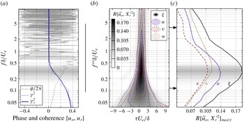
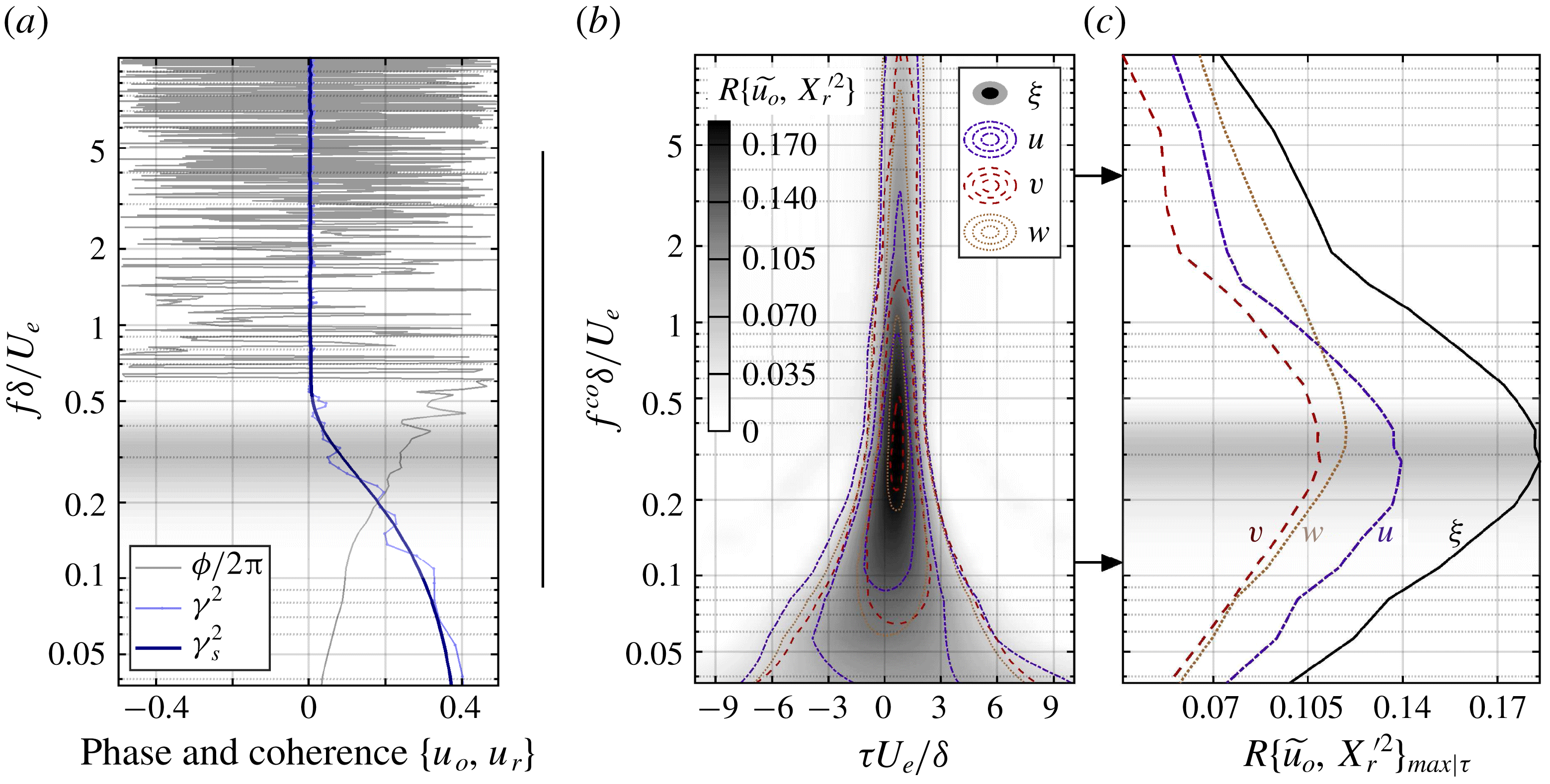
the complex logarithm. Featured in figure 8(a), both show highly coherent dynamics for frequencies up to
 $f\unicode[STIX]{x1D6FF}/U_{e}\leqslant 0.4$
, demonstrating that only large scales correlate both the roughness sublayer and the outer layer. In the roughness sublayer, it is therefore relevant to separate large scales – dominated by outer-layer-related structures – from primarily roughness-driven small-scale dynamics. Nonetheless, it should be noted that the highest level of coherence found here, approximately 0.35, is approximately half of the one reported by Baars, Hutchins & Marusic (Reference Baars, Hutchins and Marusic2016) for smooth-wall cases. Note that the coherence shown in figure 8(a) is computed between hot-wire time series at
 $z_{o}$
and SPIV streamwise series at
 $z_{r}$
, hence uses Taylor’s hypothesis of frozen turbulence. For information coherence using exclusively HWA time series reaches 0.55 for the largest scales. The lower coherence likely comes from the presence of the large-roughness wake dynamics shed above the canopy, which not only disrupts the near-wall turbulence and the smallest scales but shed motions at scales closer to the outer-layer large scales.
The phase
 $\unicode[STIX]{x1D719}\{u_{o},u_{r}\}$
can be written as a time shift
 $\unicode[STIX]{x1D70F}_{r}^{o}=\unicode[STIX]{x1D719}/2\unicode[STIX]{x03C0}f$
between the two signals
 $u_{o}$
and
 $u_{r}$
. Since
 $\unicode[STIX]{x1D719}\{u_{o},u_{r}\}$
increases fairly linearly with the frequency throughout the range of coherent dynamics, it yields a constant time shift
 $\unicode[STIX]{x1D70F}_{r}^{o}\simeq -0.80\unicode[STIX]{x1D6FF}/U_{e}$
. This provides an estimation for the average inclination of the large-scale motions between
 $15^{\circ }\leqslant \unicode[STIX]{x1D703}\leqslant 21^{\circ }$
depending on the advection velocity (between
 $U_{a}(z_{r})$
and
 $U_{a}(z_{o})$
). This angle is larger than for smooth walls, as expected for highly roughened flows (Wu & Christensen Reference Wu and Christensen2010; Lee et al.
Reference Lee, Sung and Krogstad2011).
Correlations between outer-layer and roughness-sublayer signals: (a) cross-spectrum between HWA signal
 $u_{o}(t_{\unicode[STIX]{x1D702}},y_{hw},z_{o})$
and
 $u_{r}(t_{\unicode[STIX]{x1D702}},y_{hw},z_{r})$
extracted from SPIV fields using Taylor’s hypothesis is represented by its phase
 $\unicode[STIX]{x1D719}$
and the magnitude squared coherence (raw,
 $\unicode[STIX]{x1D6FE}^{2}$
and smoothed,
 $\unicode[STIX]{x1D6FE}_{s}^{2}$
) against dimensionless frequency
 $f\unicode[STIX]{x1D6FF}/U_{e}$
. PSDs are computed over 600, 50 %-overlapped 10s-long windows; on the right, cross-correlation coefficients
 $R\{\widetilde{u_{o}},X_{r}^{\prime 2}\}$
(4.3) between large-scale signal
 $\widetilde{u_{o}}$
and roughness-sublayer small-scale kinetic energy terms as functions of the cutoff frequency
 $f^{co}\unicode[STIX]{x1D6FF}/U_{e}$
, (b) maps depending on time delay and (c) profiles of maximal correlation
 $R\{\widetilde{u_{o}},X_{r}^{\prime 2}\}_{max|\unicode[STIX]{x1D70F}}$
.
4.2 Scale interactions and choice of cutoff frequency
In order to investigate the nonlinear influence of the large-scale motions on small-scale turbulence, the flow is split into coherent dynamics on one hand and so-called stochastic fluctuations on the other hand. Following that approach Blackman & Perret (Reference Blackman and Perret2016) recently used linear stochastic estimation to identify the large-scale dynamics measured by PIV in the vicinity of the canopy that was coherent with fluctuations measured much higher in the log region. The results showed the occurrence of amplitude modulation for all three velocity components in the roughness sublayer, less so within the canopy flow. A spectral counterpart to this approach was introduced by Baars et al. (Reference Baars, Hutchins and Marusic2016) in the case of a smooth-wall boundary layer. These methods are attractive because they provide a decomposition based on physics only, the sole arbitrary choice being the threshold above which fluctuations are considered as coherent (a coherence of 0.05 in Baars et al. (Reference Baars, Hutchins and Marusic2016)). On the other hand, results can therefore be particularly sensitive to the distance between the two sources in the outer region and closer to the wall since coherence levels depend significantly on that distance. The authors discuss that aspect in Perret et al. (Reference Perret, Basley, Mathis and Piquet2018) in which they apply spectral stochastic estimation to the same flow as that of the present work, using a wall-normal distribution of hot-wire measurements. Another limitation of the coherence-based scale-separation methods comes from the symmetry properties of the flow, which cause a drop of coherence between spanwise velocity and any other quantity when spanwise shift approaches zero. As the present study aims to expand scale separation consistently to all terms of kinetic energy, the decomposition must occur invariably regardless of the velocity component under study. Low-pass filtering is more reliable in that respect and is, incidentally, most often employed in the literature to reveal the large-scale modulation of small scales (Mathis et al.
Reference Mathis, Hutchins and Marusic2009; Harun et al.
Reference Harun, Monty, Mathis and Marusic2013; Squire et al.
Reference Squire, Baars, Hutchins and Marusic2016a
; Yao et al.
Reference Yao, Huang and Xu2018, for instance). The fluctuating flow is hence split into large-scale dynamics
 $\widetilde{\boldsymbol{u}}$
and small-scale fluctuations
 $\boldsymbol{u}^{\prime }$
using a low-pass gate function
 $g(t)$
of cutoff frequency
 $f^{co}$
,
 $$\begin{eqnarray}\boldsymbol{u}=\widetilde{\boldsymbol{u}}+\boldsymbol{u}^{\prime },\quad \widetilde{\boldsymbol{u}}=g\ast \boldsymbol{u},\quad \boldsymbol{u}^{\prime }=\boldsymbol{u}-\widetilde{\boldsymbol{u}}.\end{eqnarray}$$
In smooth-wall-bounded flows, the cutoff frequency/wavelength is generally chosen arbitrarily within the relatively low energy plateau separating the inner and outer peaks in wall-normal profiles of spectra of streamwise velocity (Bandyopadhyay & Hussain Reference Bandyopadhyay and Hussain1984; Hutchins & Marusic Reference Hutchins and Marusic2007b
; Mathis et al.
Reference Mathis, Hutchins and Marusic2009, Reference Mathis, Marusic, Hutchins and Sreenivasan2011b
; Ganapathisubramani et al.
Reference Ganapathisubramani, Hutchins, Monty, Chung and Marusic2012; Harun et al.
Reference Harun, Monty, Mathis and Marusic2013; Talluru et al.
Reference Talluru, Baidya, Hutchins and Marusic2014). The cutoff wavelength – Taylor’s hypothesis is considered in all cases – is typically chosen equal to
 $\unicode[STIX]{x1D706}^{co}\sim \unicode[STIX]{x1D6FF}$
. With high Reynolds numbers, the interval between the near-wall and outer regions broadens significantly so that changing the cutoff was shown by Mathis et al. (Reference Mathis, Hutchins and Marusic2009) and Ganapathisubramani et al. (Reference Ganapathisubramani, Hutchins, Monty, Chung and Marusic2012) to have little influence on the occurrence of modulation. On the other hand, high-roughness interference entails much larger scales in the roughness sublayer relatively to those of the near-wall inner layer, hereby drastically reducing the difference with outer-layer scales. The analysis of the modulation of small-scale turbulence hence becomes more sensitive to cutoff frequency than over a smooth wall.
We propose to search for the most relevant cutoff frequency
 $f^{co}$
that separates modulated from modulating dynamics using a parametric study on third-order moments. Mathis et al. (Reference Mathis, Marusic, Hutchins and Sreenivasan2011b
) demonstrated that the cross-term
 $3\langle \widetilde{u}u^{\prime 2}\rangle$
in the decomposed skewness
 $\langle u^{3}\rangle =\langle \widetilde{u}^{3}\rangle +3\langle \widetilde{u}^{2}u^{\prime }\rangle +3\langle \widetilde{u}u^{\prime 2}\rangle +\langle u^{\prime 3}\rangle$
is directly related to the degree of AM. The connection between skewness and amplitude modulation has been investigated in many studies since, for instance in Agostini, Leschziner & Gaitonde (Reference Agostini, Leschziner and Gaitonde2016). The quantity
 $\langle \widetilde{u}u^{\prime 2}\rangle$
represents the single-point non-delayed correlation between large-scale fluctuations
 $\widetilde{u}$
and small-scale Reynolds stress
 $u^{\prime 2}$
. Here we expand this approach to include third-order moments involving large-scale fluctuations in the outer layer and small-scale kinetic energy in the roughness sublayer, namely
 $\widetilde{u_{o}}\unicode[STIX]{x1D709}_{r}^{\prime 2}$
,
 $\widetilde{u_{o}}u_{r}^{\prime 2}$
,
 $\widetilde{u_{o}}v_{r}^{\prime 2}$
and
 $\widetilde{u_{o}}w_{r}^{\prime 2}$
. To take into account the time shift
 $\unicode[STIX]{x1D70F}$
between signals, time averages are replaced by correlation coefficients
 $$\begin{eqnarray}R\{\widetilde{u_{o}},X_{r}^{\prime 2}\}(\unicode[STIX]{x1D70F},f^{co})=\frac{\langle \widetilde{u_{o}}(t_{\unicode[STIX]{x1D702}},f^{co})\,X_{r}^{\prime 2}(t_{\unicode[STIX]{x1D702}}+\unicode[STIX]{x1D70F},f^{co})\rangle }{\unicode[STIX]{x1D70E}_{\widetilde{u_{o}}}\unicode[STIX]{x1D70E}_{X_{r}^{\prime 2}}},\quad X_{r}^{\prime 2}=\{\unicode[STIX]{x1D709}_{r}^{\prime 2},u_{r}^{\prime 2},v_{r}^{\prime 2},w_{r}^{\prime 2}\},\end{eqnarray}$$
where
 $\unicode[STIX]{x1D70E}$
denotes a standard deviation (figure 8
b). It is important to point out the significance of these correlation coefficients
 $R\{\widetilde{u_{o}},X_{r}^{\prime 2}\}$
: (i) they relate dynamics at distant wall-normal locations (
 $z_{o}-z_{r}>0.15\unicode[STIX]{x1D6FF}$
); (ii) the two unfiltered signals contain entirely different ranges of scales: by definition, only the large-scale part of the roughness-sublayer kinetic energy terms can potentially participate to the correlation with the outer-layer dynamics, resulting in relatively low coefficient; (iii) HWA time series at
 $z_{o}$
and reconstructed streamwise strips at
 $z_{r}$
can only be correlated by considering Taylor’s hypothesis. The correlation levels are well above noise level and of the same order as in Blackman & Perret (Reference Blackman and Perret2016) (between 0.15 and 0.2) or Anderson (Reference Anderson2016), who investigated the amplitude modulation of streamwise velocity fluctuations in the roughness sublayer via LES performed in a similar wall configuration as in the present study. The level of these correlation coefficients is also in agreement with those reported in turbulent boundary layers over smooth walls (above
 $z^{+}=20$
) by Mathis et al. (Reference Mathis, Marusic, Hutchins and Sreenivasan2011b
).
Outer-layer large-scale motions (
 $\widetilde{u_{o}}$
) statistically precede roughness-sublayer kinetic energy fluctuations (
 $\unicode[STIX]{x1D709}_{r}^{\prime 2}$
) by
 $\unicode[STIX]{x1D70F}\{\widetilde{u_{o}},X_{r}^{\prime 2}\}\simeq 0.6\unicode[STIX]{x1D6FF}/U_{e}$
. Bandyopadhyay & Hussain (Reference Bandyopadhyay and Hussain1984) pointed out the significant change of the time shift across the boundary layer. This is due to the inclination of the streaky large-scale motions. Numerous works investigated the evolution of correlation between near-wall small-scale dynamics and large-scale motions at decreasing wall-distance (Guala, Metzger & McKeon Reference Guala, Metzger and McKeon2011; Ganapathisubramani et al.
Reference Ganapathisubramani, Hutchins, Monty, Chung and Marusic2012; Talluru et al.
Reference Talluru, Baidya, Hutchins and Marusic2014; Baars et al.
Reference Baars, Hutchins and Marusic2017, for instance). They have shown that small-scale dynamics modulation is actually shifted forward when considering its local large-scale counterpart (Mathis et al.
Reference Mathis, Hutchins and Marusic2011a
). This will be discussed in detail in § 5.
The maximum of correlation coefficients
 $R\{\widetilde{u_{o}},X_{r}^{\prime 2}\}$
is reached for cutoff frequencies around
 $0.2\leqslant f^{co}\unicode[STIX]{x1D6FF}/U_{e}\leqslant 0.4$
. The spectral content of each component being different, it is then natural that each Reynolds stress does not produce strictly the same correlation with the large-scale streamwise velocity. It is worthwhile noting that these frequencies correspond to those below which outer layer and roughness sublayer lose their coherence (figure 8
a). This confirms the correlation between outer-layer fluctuations and roughness small-scale energy is a good criterion to separate outer-layer-related dynamics from that intrinsic to the roughness sublayer.
In order to avoid the use of multiple cutoff frequencies depending on the velocity component, which could have made the analysis unnecessarily complex, we choose to perform the scale decomposition using
 $f^{co}\simeq 0.3U_{e}/\unicode[STIX]{x1D6FF}$
, the cutoff frequency for which the third-order correlation coefficient
 $R\{\widetilde{u_{o}},\unicode[STIX]{x1D709}_{r}^{\prime 2}\}$
is maximal. Note however that any cutoff frequency chosen in the range
 $0.2\leqslant f^{co}\unicode[STIX]{x1D6FF}/U_{e}\leqslant 0.5$
would produce qualitatively the same outcome. The frequency
 $f^{co}$
corresponds to streamwise wavelengths
 $\unicode[STIX]{x1D706}_{x}^{co}(z_{r})=U_{a}(z_{r})/f^{co}=1.66\unicode[STIX]{x1D6FF}$
and
 $\unicode[STIX]{x1D706}_{x}^{co}(z_{o})=U_{a}(z_{o})/f^{co}=2.36\unicode[STIX]{x1D6FF}$
. It is important to observe that spanwise and wall-normal components are almost entirely cut off by the low-pass decomposition. In other words, all dynamics carried by
 $v$
and
 $w$
are recovered in the small-scale part of the decomposition and are modulated by the large-scale motions. One may refer to the wavelet spectra plotted in figure 7 for an illustration of that result.
4.3 Large-scale evolution of kinetic energy: amplitude modulation coefficients
The amplitude modulation of the small-scale turbulence embodies the large-scale evolution of the intensity of small-scale dynamics, in phase with fluctuations associated with the large-scale motions of the flow. Various methods have been employed to extract the envelope (or instantaneous amplitude) of the small-scale turbulence in wall-bounded flows. After fluctuating velocity signals are split into small-scale and large-scale components (4.2), the Hilbert transform of the small-scale velocity is commonly employed since Mathis et al. (Reference Mathis, Hutchins and Marusic2009) to build an analytic signal whose envelope is extracted. Note that Hilbert transform is also at the core of the empirical mode decomposition used in Agostini & Leschziner (Reference Agostini and Leschziner2014) and Agostini et al. (Reference Agostini, Leschziner and Gaitonde2016). Recently Baars et al. (Reference Baars, Talluru, Hutchins and Marusic2015, Reference Baars, Hutchins and Marusic2017) introduced a procedure in which the instantaneous amplitude is obtained via wavelet spectra. Alternatively, amplitude modulation can be observed through Reynolds stresses, like Ganapathisubramani et al. (Reference Ganapathisubramani, Hutchins, Monty, Chung and Marusic2012) and Talluru et al. (Reference Talluru, Baidya, Hutchins and Marusic2014). The authors have applied these methods on the data presented here and all produce strikingly similar results. The forthcoming analysis uses Reynolds stresses since access to all three velocity components allows us to investigate small-scale energy, namely
 $\unicode[STIX]{x1D709}_{r}^{\prime 2}=(u_{r}^{\prime 2}+v_{r}^{\prime 2}+w_{r}^{\prime 2})/2$
, a Galilean invariant.
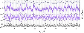
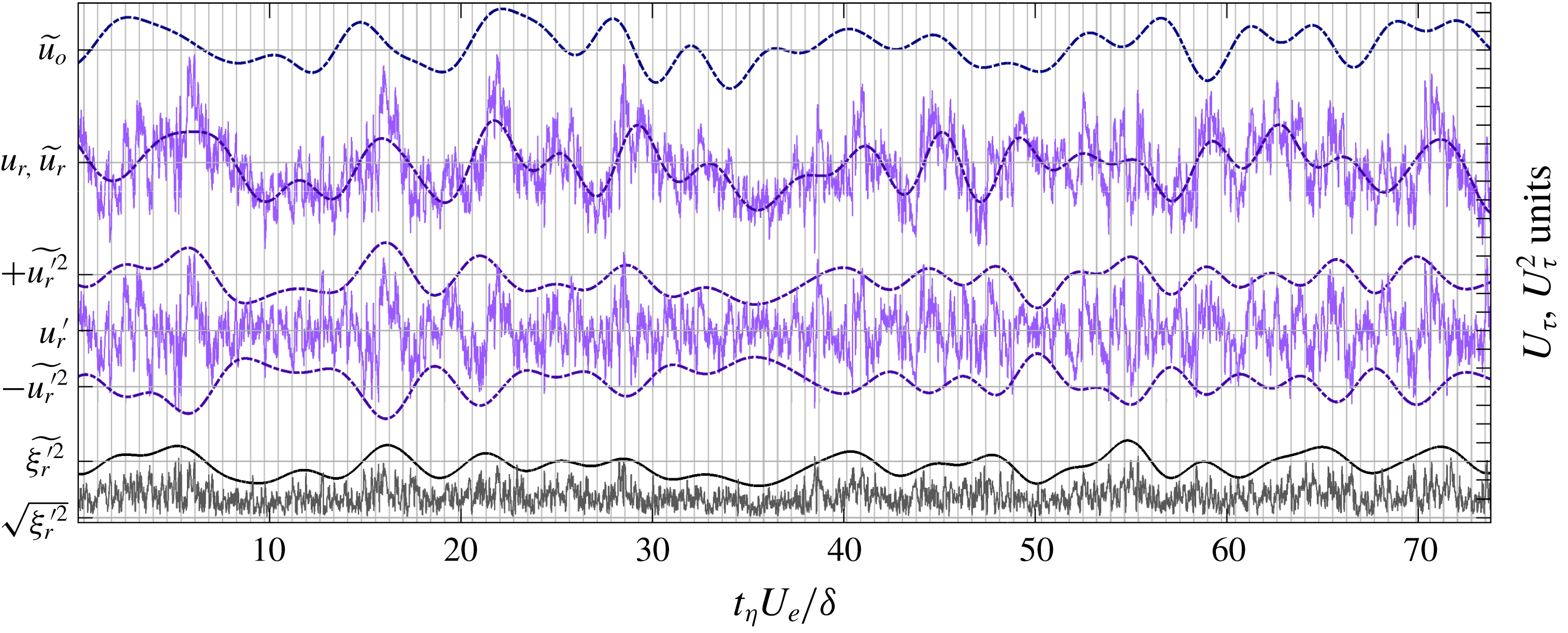
Illustration of scale decomposition with cutoff frequency
 $f^{co}=0.3\,U_{e}/\unicode[STIX]{x1D6FF}$
: from top to bottom, HWA large-scale time series
 $\widetilde{u_{o}}$
measured at
 $z_{o}=5.0h$
,
 $u_{r}(t_{\unicode[STIX]{x1D702}},y_{hw})$
extracted from combined SPIV fields at
 $z_{r}=1.5h$
is split into
 $\widetilde{u_{r}}$
and
 $u_{r}^{\prime }$
, whose large-scale envelope
 $\widetilde{u_{r}^{\prime 2}}$
is identified. Total small-scale kinetic energy fluctuations are also plotted in the form of
 $\sqrt{\unicode[STIX]{x1D709}_{r}^{\prime 2}(t_{\unicode[STIX]{x1D702}},y_{hw})}$
and the envelope
 $\widetilde{\unicode[STIX]{x1D709}_{r}^{\prime 2}}$
. Velocities are normalised by
 $U_{\unicode[STIX]{x1D70F}}$
and envelopes of kinetic energies by
 $U_{\unicode[STIX]{x1D70F}}^{2}$
. Vertical lines mark the junctions between SPIV fields.
The large-scale evolution of the small-scale kinetic energy is extracted in order to be compared to large-scale motions and to quantify its level of amplitude modulation. This is achieved using the same low-pass filtering as previously
 $$\begin{eqnarray}\widetilde{X_{r}^{\prime 2}}=g\ast X_{r}^{\prime 2},\quad X_{r}^{\prime 2}=\{\unicode[STIX]{x1D709}_{r}^{\prime 2},u_{r}^{\prime 2},v_{r}^{\prime 2},w_{r}^{\prime 2}\}.\end{eqnarray}$$
Illustration of the scale decomposition is featured in figure 9. It shows that large-scale motions are organised in high and low momentum regions (HMRs and LMRs) leading to, respectively, high and low fluctuations of the streamwise velocity component. They are identified both in the outer layer and in the roughness sublayer by the large-scale signals
 $\widetilde{u_{o}}$
and
 $\widetilde{u_{r}}$
, respectively. Figure 9 also shows how
 $\widetilde{u_{o}}$
and
 $\widetilde{u_{r}}$
are strongly correlated with the evolution of the small-scale kinetic energy in the roughness sublayer. These findings confirm LES results by Anderson (Reference Anderson2016) and are strikingly similar to those of smooth-wall cases (Marusic et al.
Reference Marusic, Mathis and Hutchins2010; Baars et al.
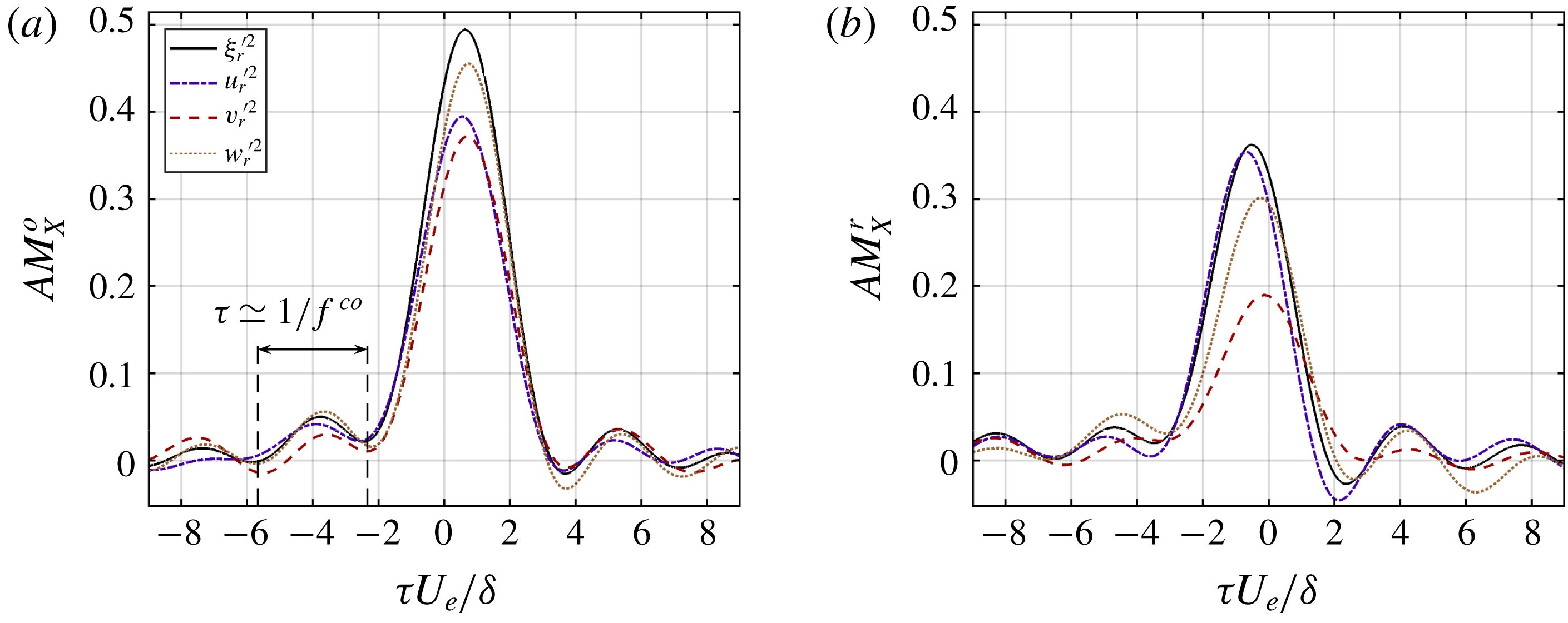
Reference Baars, Hutchins and Marusic2017). To quantify the degree of amplitude modulation, Mathis et al. (Reference Mathis, Hutchins and Marusic2009) defined the amplitude modulation coefficient as the correlation coefficient between the large-scale fluctuations of streamwise velocity and the large-scale envelope of the small scales in the near-wall region. This definition can be generalised to time-delayed correlations:
 $$\begin{eqnarray}AM_{X}^{o}(\unicode[STIX]{x1D70F})=\frac{\langle \widetilde{u_{o}}(t_{\unicode[STIX]{x1D702}})\,\widetilde{X_{r}^{\prime 2}}(t_{\unicode[STIX]{x1D702}}+\unicode[STIX]{x1D70F})\rangle }{\unicode[STIX]{x1D70E}_{\widetilde{u_{o}}}\unicode[STIX]{x1D70E}_{\widetilde{X_{r}^{\prime 2}}}},\quad AM_{X}^{r}(\unicode[STIX]{x1D70F})=\frac{\langle \widetilde{u_{r}}(t_{\unicode[STIX]{x1D702}})\,\widetilde{X_{r}^{\prime 2}}(t_{\unicode[STIX]{x1D702}}+\unicode[STIX]{x1D70F})\rangle }{\unicode[STIX]{x1D70E}_{\widetilde{u_{r}}}\unicode[STIX]{x1D70E}_{\widetilde{X_{r}^{\prime 2}}}},\end{eqnarray}$$
that are plotted against time shift
 $\unicode[STIX]{x1D70F}$
in figure 10. Coefficients
 $AM^{o}$
quantify the (global) amplitude modulation by large-scale motions taken in the outer layer (
 $\widetilde{u_{o}}$
) whereas coefficients
 $AM^{r}$
are single-point correlation coefficients, which convey the modulation by the local imprint of the large-scale motions in the roughness sublayer (
 $\widetilde{u_{r}}$
). The time shift defined by the salient peak of correlation is different depending on whether one considers the modulation by the outer-layer dynamics or the local large-scale signal, due to the inclination of the large-scale structures, mentioned earlier in § 4.1.
Before comparing these results to the smooth-wall case, one must remember that Mathis et al. (Reference Mathis, Hutchins and Marusic2009) and Marusic et al. (Reference Marusic, Mathis and Hutchins2010) extracted the small-scale signal at the inner peak location, typically around
 $z^{+}=15$
in turbulent boundary layers over smooth walls. High roughness invalidates this organisation and expands drastically the inner region. As a result small-scale fluctuations are here measured at the core of the roughness sublayer, that is much higher in wall units (
 $z_{r}^{+}\simeq 2130$
). And yet,
 $AM$
coefficients unambiguously indicate a spike of amplitude modulation as strong as that of the smooth-wall case, as predicted by the LES of Anderson (Reference Anderson2016). One observes high levels of amplitude modulation across all kinetic energy terms, as expected from Talluru et al. (Reference Talluru, Baidya, Hutchins and Marusic2014) and Blackman & Perret (Reference Blackman and Perret2016), but with different levels of modulation between components. While streamwise velocity is amplitude modulated both locally and globally at similar levels (around 0.4), the other components present higher
 $AM^{o}$
coefficients than
 $AM^{r}$
. It is worth noting that the amplitude modulation on the total kinetic energy is always more pronounced than any of its constitutive terms. This integrated effect is explained by considering coherent structures, whose projection on
 $(x,y,z)$
axes obviously varies in time and space. While modulation might not be observed in the fluctuations of a given velocity component, the inter-scale exchange mechanism affects globally the coherent structures themselves.
The time shift of the main peak varies also significantly from one velocity component to another. Figure 10(b) reveals that contrary to the streamwise velocity that is locally forward in phase relatively to the large-scale motion, spanwise and wall-normal Reynolds stresses are modulated with almost no time shift.
In the next section we demonstrate that the difference in phase is in fact due to the bidimensional organisation in the wall-parallel plane of the AM mechanism for which the maxima of modulation of the spanwise and wall-normal velocity components occur preferentially on the flanks of the large-scale motions while the small scales of the streamwise velocity component are modulated on the upstream front of the large-scale motions. Finally, one may notice beside the main peak the presence of oscillations for both
 $AM^{o}$
and
 $AM^{r}$
. These oscillations at a period of
 $\unicode[STIX]{x1D70F}U_{e}/\unicode[STIX]{x1D6FF}\simeq 3.3$
are caused by the low-pass filter cutting through the broadband signature of large-scale dynamics.
Amplitude modulation coefficients of the kinetic energy terms
 $X_{r}^{\prime 2}=\{\unicode[STIX]{x1D709}_{r}^{\prime 2},u_{r}^{\prime 2},v_{r}^{\prime 2},w_{r}^{\prime 2}\}$
, (a)
 $AM_{X}^{o}$
by the outer-layer large-scale signal and (b),
 $AM_{X}^{r}$
by the local large-scale signal, as functions of time shift
 $\unicode[STIX]{x1D70F}U_{e}/\unicode[STIX]{x1D6FF}$
. Scale separation is performed at cutoff frequency
 $f^{co}=0.3U_{e}/\unicode[STIX]{x1D6FF}$
.

5 Spatial imprint of the large-scale modulations
The literature discussing modulation by LSMs has mainly focused on the wall-normal distribution of the modulation coefficients (Mathis et al.
Reference Mathis, Marusic, Hutchins and Sreenivasan2011b
; Baars et al.
Reference Baars, Talluru, Hutchins and Marusic2015, Reference Baars, Hutchins and Marusic2017; Nadeem et al.
Reference Nadeem, Lee, Lee and Sung2015; Anderson Reference Anderson2016; Blackman & Perret Reference Blackman and Perret2016). It is now well known that the modulation concentrates in the inner region and is locally phase forward with respect to the large-scale fluctuations. In contrast, the wall-parallel organisation of the modulation – spanwise in particular – has only been investigated once, in the smooth-wall case, by Talluru et al. (Reference Talluru, Baidya, Hutchins and Marusic2014). This section characterises the local imprint of the phenomenon within the roughness sublayer, using bidimensional maps of
 $AM$
coefficients in the
 $xy$
-plane at wall distance
 $z_{r}=1.5h$
.
5.1 Scale decomposition in wall-parallel plane
 $z_{r}=1.5h$

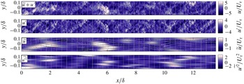
Illustration of the scale decomposition in the roughness sublayer with cutoff wavelength
 $\unicode[STIX]{x1D706}_{x}^{co}=1.66\unicode[STIX]{x1D6FF}$
: excerpt out of combined SPIV fields in plane
 $z_{r}=1.5h$
with, from top to bottom, the fluctuations of streamwise velocity component
 $u$
, the small-scale part
 $u^{\prime }$
only, the large-scale part
 $\widetilde{u}$
(vectors depict the large-scale velocity field
 $\widetilde{u}\boldsymbol{e}_{x}+\widetilde{v}\boldsymbol{e}_{y}$
), and the large-scale envelope of Reynolds stress
 $\widetilde{u^{\prime 2}}$
.

The scale decomposition performed over time series in § 4 can be applied to whole Taylor-combined SPIV fields, hereby identifying the large-scale motions, the small-scale fluctuations and their large-scale envelope in a two-dimensional extension (figure 11). It should be emphasised that low-pass filtering is only performed streamwise, along
 $\unicode[STIX]{x1D702}$
, using the cutoff wavelength
 $\unicode[STIX]{x1D706}_{x}^{co}(z_{r})=U_{a}(z_{r})/f^{co}=1.66\unicode[STIX]{x1D6FF}$
. The spatial coherence of large-scale motions ensures an intrinsic spanwise scale decomposition. Note that from now on, the analysis is restricted to the plane
 $z_{r}=1.5h$
and notations are simplified (
 $u_{r}\rightarrow u$
,
 $\unicode[STIX]{x1D709}_{r}^{2}\rightarrow \unicode[STIX]{x1D709}^{2}$
, etc.).
Although one could expect a pronounced signature of the cubes at such wall-normal location close to the canopy (
 $z_{r}=1.5h$
), the convective nature of the flow and the high turbulence intensity have already scattered most of the roughness-shed fluctuations. This justifies the applicability of the modulation mechanism, in spite of the heterogeneity induced by the high roughness. From a visual inspection of figure 11, an undeniable correspondence between
 $\widetilde{u}$
and
 $\widetilde{u^{\prime 2}}$
can indeed be observed.
5.2 Spatial modulation around large-scale motions
Amplitude modulation coefficients can be defined by both streamwise and spanwise two-point correlations, i.e. in the wall-parallel plane at
 $z_{r}=1.5h$
 $$\begin{eqnarray}AM_{X}(\unicode[STIX]{x1D6E5}_{x},\unicode[STIX]{x1D6E5}_{y})=R\{\widetilde{u},\widetilde{X^{\prime 2}}\}=\frac{\langle \widetilde{u}(\unicode[STIX]{x1D702},y)\,\widetilde{X^{\prime 2}}(\unicode[STIX]{x1D702}+\unicode[STIX]{x1D6E5}_{x},y+\unicode[STIX]{x1D6E5}_{y})\rangle _{\unicode[STIX]{x1D702},y}}{\unicode[STIX]{x1D70E}_{\widetilde{u}}\unicode[STIX]{x1D70E}_{\widetilde{X^{\prime 2}}}},\end{eqnarray}$$
as opposed to wall-normal correlations presented in § 4.3 and in Mathis et al. (Reference Mathis, Marusic, Hutchins and Sreenivasan2011b
). Note here that
 $\widetilde{u}(\unicode[STIX]{x1D702},y)$
is the local large-scale imprint of the outer-layer large scales as observed in the roughness sublayer at
 $z_{r}$
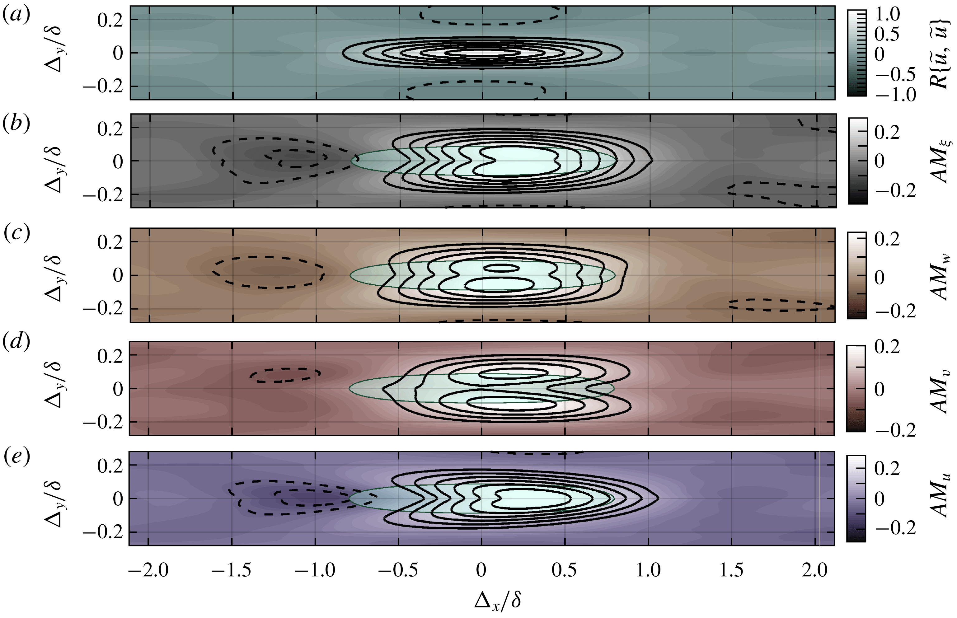
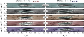
. This is equivalent to a one-point correlation in the wall-normal direction as opposed to the two-point correlation used in (4.5). The resulting AM maps are shown in figure 12(b–e). They represent the spatial distribution of amplitude modulation of the small-scale dynamics with respect to the LSMs associated with
 $\widetilde{u}$
fluctuations. Figure 12(b–e) indicates that the kinetic energy modulations are statistically phase forward to LSMs – about
 $\unicode[STIX]{x1D6E5}_{x}\simeq 0.25\unicode[STIX]{x1D6FF}$
upstream – as previously observed (Talluru et al.
Reference Talluru, Baidya, Hutchins and Marusic2014; Baars et al.
Reference Baars, Talluru, Hutchins and Marusic2015). Moreover, the AM is more intense along the edges of the LSMs, with the presence of two lobes on both sides (spanwise) of auto-correlation peak
 $R\{\widetilde{u},\widetilde{u}\}$
. This organisation combines the three terms of kinetic energy, which exhibit very different modulation patterns. It is worth noting that two-point correlation maps in figure 12 integrate all large-scale events – both low and high momentum regions (LMRs and HMRs) – and the spanwise symmetry of the flow. The meandering nature of LSMs and its local impact on the distribution of AM coefficients cannot be identified this way.
Two-point correlation maps in plane
 $z_{r}=1.5h$
for (a) auto-correlation
 $R\{\widetilde{u},\widetilde{u}\}$
, (b–e) amplitude modulation coefficients
 $AM_{\unicode[STIX]{x1D709}}=R\{\widetilde{u},\widetilde{\unicode[STIX]{x1D709}^{\prime 2}}\}$
,
 $AM_{w}=R\{\widetilde{u},\widetilde{w^{\prime 2}}\}$
,
 $AM_{v}=R\{\widetilde{u},\widetilde{v^{\prime 2}}\}$
,
 $AM_{u}=R\{\widetilde{u},\widetilde{u^{\prime 2}}\}$
, respectively, shaded cyan areas delimit
 $R\{\widetilde{u},\widetilde{u}\}\geqslant 0.2$
in each case. Plain (dashed) contours depict positive (negative) iso-levels for (a)
 $\pm [0.15,0.9]$
by steps of 0.15, and for (b–e)
 $\pm [0.06,0.34]$
by steps of 0.04.

Same as figure 13 with conditional analysis based on large-scale velocity field, left
 $(\widetilde{u}>0,\widetilde{v}>0)$
for high momentum regions, and right
 $(\widetilde{u}<0,\widetilde{v}<0)$
for low momentum regions. Plain (dashed) contours depict positive (negative) iso-levels
 $\pm [0.15,0.9]$
by steps of 0.15 for
 $R\{\widetilde{u},\widetilde{u}\}$
, and
 $\pm [0.06,0.34]$
by steps of 0.04 for
 $AM$
coefficients. The patterns sketched on top represent the large-scale motions selected by conditional average.
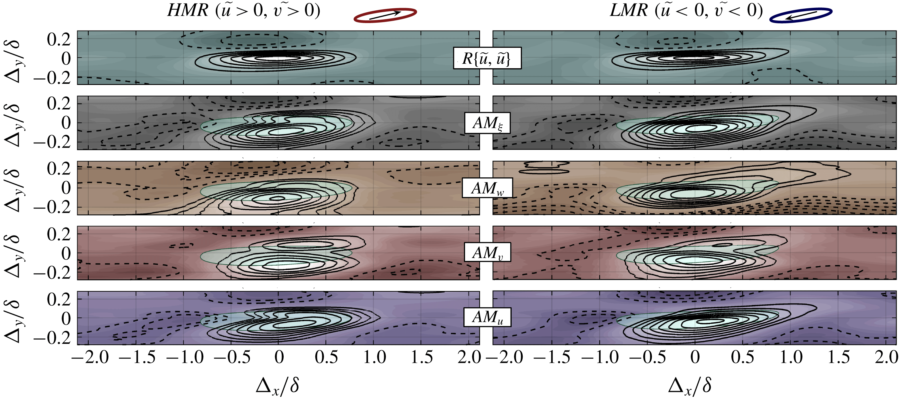
A conditional analysis is carried out on the large-scale velocity field
 $(\widetilde{u},\widetilde{v})$
to differentiate HMRs
 $(\widetilde{u}>0)$
from LMRs
 $(\widetilde{u}<0)$
. Spanwise symmetry effects are removed by a condition on the sign of the spanwise velocity component: only the HMRs where
 $(\widetilde{v}>0)$
are considered, whereas only
 $(\widetilde{v}<0)$
is considered for LMRs. The two-point correlation maps featured in figure 13 are hereby computed, on the left-hand side, using
 $(\widetilde{u}|\widetilde{u}>0;\widetilde{v}>0)$
and on the right-hand side, using
 $(\widetilde{u}|\widetilde{u}<0;\widetilde{v}<0)$
. Auto-correlation
 $R\{\widetilde{u},\widetilde{u}\}$
contours depict slightly skewed patterns which represent the meandering large-scale motions – HMRs and LMRs follow the stream
 $(\widetilde{u}>0,\widetilde{v}>0)$
and
 $(\widetilde{u}<0,\widetilde{v}<0)$
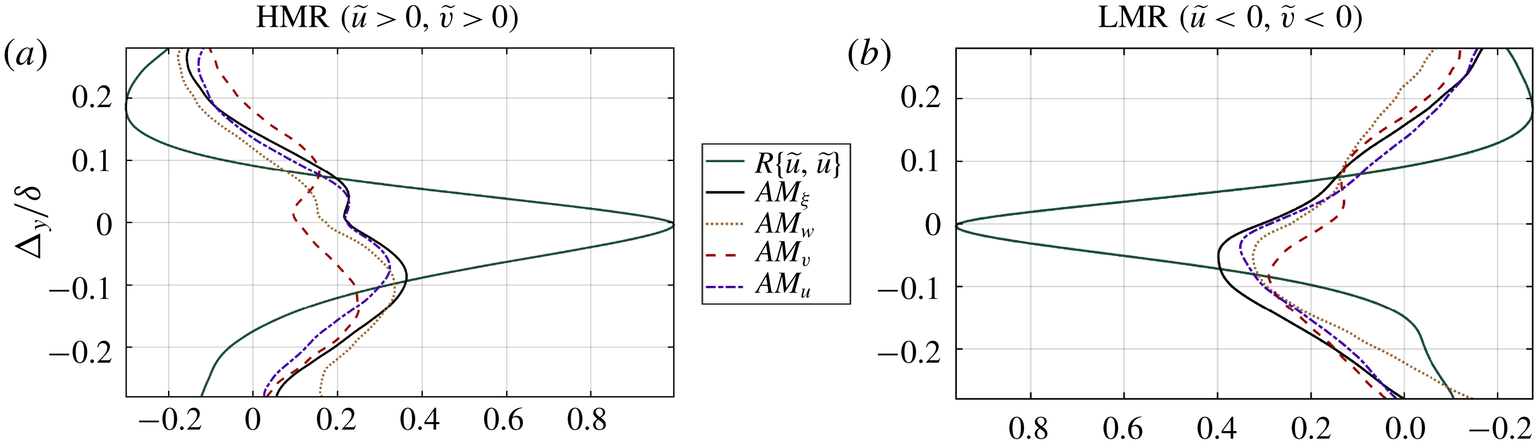
, respectively. But these structures induce much stronger asymmetries in the modulation distributions, which concentrate towards the side of the LSMs that faces upstream. This asymmetry is revealed even more strikingly in the profiles extracted from figure 13 at
 $\unicode[STIX]{x1D6E5}_{x}=0.1\unicode[STIX]{x1D6FF}$
, plotted in figure 14. Moreover, the modulation coefficients are organised differently depending on the velocity components. Streamwise velocity fluctuations
 $u^{\prime 2}$
are primarily modulated near the front of LSMs, consistent with the phase-forward time series reported in the literature. This result completes the findings of Baars et al. (Reference Baars, Hutchins and Marusic2017), who recently reported in the outer region a preferential arrangement of the modulated small-scale activity in shear layers developing both downstream and upstream of the large-scale motions. However, in the high-roughness case studied here, this preferential arrangement begins to appear at a much lower wall-normal location, in the roughness sublayer at
 $z_{r}$
. Note that the arrangement observed by Baars et al. (Reference Baars, Hutchins and Marusic2017) in the inner layer is absent since the latter has been utterly altered by the presence of roughness elements.
Spanwise profiles extracted from maps in figure 13 at
 $\unicode[STIX]{x1D6E5}_{x}=0.1\unicode[STIX]{x1D6FF}$
; (a) HMRs
 $(\widetilde{u}>0,\widetilde{v}>0)$
are plotted and (b), LMRs
 $(\widetilde{u}<0,\widetilde{v}<0)$
are shown with a reversed axis to point out the negative sign of the underlying fluctuations.

The modulations of spanwise velocity fluctuations
 $v^{\prime 2}$
and wall-normal velocity fluctuations
 $w^{\prime 2}$
shed light on the spanwise organisation of the modulation around the high momentum and low momentum regions. Reynolds stress
 $v^{\prime 2}$
is modulated in space as two lobes of equal importance attached to lateral parts of HMRs and rather asymmetrically around the LMRs. Modulations of
 $w^{\prime 2}$
are significantly shifted spanwise depending on the sign of
 $\widetilde{v}$
. The amplitude modulation of the Galilean invariant
 $\widetilde{\unicode[STIX]{x1D709}^{\prime 2}}$
integrates the contributions of all Reynolds stresses to form an arrow-shaped region of enhanced small-scale turbulence at the front of HMRs. On the other hand, the narrower LMRs are correlated with a single elongated region of reduced small-scale turbulence along one of its flank, depending on its orientation.
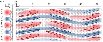
Schematic representation of the spatial organisation of the coherent structures inferred from the present AM analysis in (a) the spanwise wall-normal plane and (b) the wall-parallel plane. Red and blue shaded areas correspond to high and low momentum regions, respectively. Amplitude modulation patterns are represented by red and blue hatched regions, where small-scale kinetic energy is enhanced and reduced, respectively. The presence of large-scale streamwise vortices of positive and negative streamwise vorticity is shown via dashed arrows in the wall-normal plane.

The spatial arrangement of the amplitude modulation, evidenced here by the bidimensional
 $AM$
coefficients in the wall-parallel plane
 $z_{r}=1.5h$
, sheds light on the organisation of the dynamics in the roughness sublayer. The summary sketch proposed in figure 15 is fully consistent with the literature that associated edges of LMRs and HMRs with shear layers promoting smaller-scale turbulence. Previous analyses of the spatio-temporal organisation of the coherent structures in turbulent boundary layer flows (Kim & Adrian Reference Kim and Adrian1999; Adrian, Meinhart & Tomkins Reference Adrian, Meinhart and Tomkins2000b
; Tomkins & Adrian Reference Tomkins and Adrian2003) demonstrated that LMRs and HMRs, besides consisting of elongated meandering structures, are flanked by regions of high shear (in the horizontal plane) populated by vortical structures. These swirling motions were identified as cross-sections of hairpin vortices straddling LMRs, consistently with the model of hairpin vortex packet. These observations and interpretations were later confirmed, notably by Dennis & Nickels (Reference Dennis and Nickels2011a
,Reference Dennis and Nickels
b
) in the smooth-wall case, and by Coceal et al. (Reference Coceal, Dobre, Thomas and Belcher2007) and Inagaki & Kanda (Reference Inagaki and Kanda2010) in the case of flows developing over high-roughness (urban-like) canopies. In particular, Dennis & Nickels (Reference Dennis and Nickels2011a
,Reference Dennis and Nickels
b
) showed that hairpin vortices are most of the time non-symmetric coherent structures arranging preferentially around LMRs, and accompanied by ejection motions laterally inclined (i.e. with a non-zero spanwise velocity fluctuation). The preferred spatial organisation tying ejections to the flank of LMRs has been further confirmed by Inagaki & Kanda (Reference Inagaki and Kanda2010) in their experimental study of boundary layers over cube arrays. Additionally, alternate LMRs and HMRs have been associated with up and downward motions, respectively, generating large-scale streamwise-axis vortices. One may refer to Zhong et al. (Reference Zhong, Li, Chen and Wang2015) or Barros & Christensen (Reference Barros and Christensen2014) in the cases of smooth open channel flows and boundary layers over irregular small roughness, respectively. This large-scale organisation – featured in figure 15(a) – highlights further the role of large-scale structures in generating regions of shear at their interfaces thereby influencing the small-scale turbulent activity.
6 Conclusions
An experimental study of an urban-type atmospheric surface layer was carried out to uncover the spatial imprint of the amplitude modulation of small-scale turbulence by large-scale motions. Large field SPIV data were obtained across a wall-parallel plane inside the roughness sublayer and was synchronised with HWA measurements to access the coherence with outer-layer large-scale dynamics. A novel method based on correlations associated with (cubic) exchange terms was proposed to identify the relevant cutoff frequency prior to performing the scale decomposition, and results are consistent with existing literature dealing with both smooth and rough walls.
The three-component velocity fields were utilised to explore spatially the degree of amplitude modulation for all terms of the fluctuating kinetic energy. The analysis notably relied on conditionally averaged two-point correlations between large-scale fluctuations of streamwise velocity and small-scale energy terms. While the literature has been focusing on the streamwise–wall-normal plane, the present study used a wall-parallel plane to extend the
 $AM$
coefficients to spanwise correlations. The patterns of
 $AM$
coefficients revealed significant differences depending on the velocity component considered. On one hand, amplitude modulation was confirmed to represent the enhancement of small-scale turbulence at the front edges of the high momentum regions and its damping at those of the low momentum regions when considering the streamwise velocity component. On the other hand, the
 $AM$
maps associated with both spanwise and wall-normal velocity components demonstrated the key role played by the regions of shear existing between HMRs and LMRs – especially on the flanks of LMRs – in promoting or damping small-scale turbulence, respectively. By cancelling the usual statistical homogeneity in the spanwise direction of boundary layer flows, conditional
 $AM$
maps based on the sign of the large-scale spanwise velocity component showed that the location of amplitude modulation patterns is tied to the meandering motion of the largest structures (figure 15). Incidentally, the streamwise-elongated shape of the large-scale structures of the outer layer was shown to leave its imprint onto the near-canopy turbulence. These findings unravel the preferential spatial organisation of small-scale dynamics around low and high momentum regions in the roughness sublayer. This establishes a direct connection between the amplitude modulation mechanism and the distribution of coherent structures into hairpin vortex packets straddling LMRs and HMRs, as proposed in the literature.
More insights into the inter-scale interplay and exchanges could come from the extension of this methodology to other Galilean invariants, such as swirling strength, in order to track coherent structures and access directly to the dynamics without any projection effects. Ultimately these findings open a path towards a space-extended generalisation of the inner–outer interactions models in wall turbulence (Marusic et al. Reference Marusic, Mathis and Hutchins2010; Baars et al. Reference Baars, Hutchins and Marusic2016; Squire et al. Reference Squire, Baars, Hutchins and Marusic2016a ) that can account for the complex spatial organisation of the coherent structures in the near-wall region. In the frame of large-eddy simulations such capability would allow for the derivation of more accurate dynamic wall models driven by unsteady large-scale motions in the outer layer.
Acknowledgements
The authors are grateful to the reviewers for their insightful remarks which helped expand the scope of the paper, and to Mr Th. Piquet for his valued technical support. This work was funded by Agence Nationale pour la Recherche (Urbanturb grant ANR-14-CE22-0012-01).
Appendix. Spatial variation of the statistics in and outside the roughness sublayer
The SPIV campaign was carried out for two wall-parallel planes, at
 $z_{r}=1.5h$
and
 $z=4.0h$
. The latter location is not mentioned above but brings information regarding the extent of the roughness sublayer. Figure 16 presents the spatial standard deviation of statistical moments in order to quantify the heterogeneity of the flow properties at both wall distances. Statistics exhibit a limited yet unambiguous heterogeneity at
 $z_{r}$
(for wall-normal shear stress in particular). On the contrary all statistics are fairly uniform at
 $z=4h$
. This demonstrates that the roughness sublayer ends between
 $z=1.5h$
and
 $z=4h$
. The reference time-series acquired at
 $z_{o}=5.0h$
therefore capture the dynamics outside the roughness layer.
Spatial standard deviation
 $\sqrt{\overline{(q-\overline{q})}^{2}}$
of a quantity
 $q$
at wall distances
 $z_{r}=1.5h$
(dark) and
 $z=4.0h$
(light): for streamwise mean velocity, Reynolds stresses and skewnesses.