





Nomenclature
Acronyms
- ADS-B
-
Automatic Dependent Surveillance - Broadcast
- BBFM2
-
Boeing Fuel Flow Model, Version 2
- CAMS
-
Copernicus Atmosphere Monitoring Service
- ICAO24
-
24-bit aircraft address
- FASM
-
fuel/available-seat/n-mile
- LAEQ
-
equivalent sound level, dBA
- LTO
-
landing and take-off operations
- TCDS
-
type certificate data sheets
- nVPM
-
non-volatile particulate matter
- VOC
-
volatile organic compound
Roman symbols
-
 $a_i$
,
$b_i$
,
$c_i$
-
constant coefficients
-
$E_1$
,
$E_2$
-
actual fuel burn and emissions
-
$M$
-
flight Mach number
-
$N1\%$
-
engine speed/throttle, percent
-
$p$
-
pressure (engine or outside air)
-
$T$
-
absolute temperature
-
$W_1$
-
mass flow rate
-
$W_f$
-
mass of fuel burn
-
$x, x_o, x_1, X$
-
distance flown


1.0 Introduction
International air traffic is governed by the International Civil Aviation Organization (ICAO) Freedoms of the Air agreement, which has been in place for many years, when air traffic was a small fraction of what it is today (ICAO Convention of 1944). Chapter II, Article 5 of the original declaration, makes explicit reference to `transit non-stop across [each contracting State] territory’.
With the exception of war zones, or where there are international disputes requiring lengthy detours, these freedoms are the basic arrangements for domestic and international flight today. In fact, flights over hostile territory for military purposes were of utmost importance in the Cold War [Reference Boyne1], and it was the primary action to take a look at unknown territory before the advent of satellite technology. A report from the 1990s signalled a shift, stating that `While [U.S.] technology would allow us to overfly countries that have no credible air defences, it is a violation of international law to do so …’ [Reference Geraci2].
Even today, it is possible to find large areas of signal absence in such areas at relatively short notice; Global Positioning System (GPS) jamming and spoofing are some of those reasons. Overcharges for overflights in certain regions are not uncommon, for example, flights over the Siberian region in the 2010s [Reference Carparelli3]. There have been questions of sovereignty over the airspace, but these are for international law to judge. The thesis by Stewart [Reference Stewart4] highlights the problem from a legal framework. An extensive bibliography is reported in the same work, including treaties and United Nations documents.
In all international agreements, there is nothing regarding environmental effects, as the research is limited to navigational aspects, aside from international laws. In particular, there is no reference to the upper control zone (above 24,500 feet); local authorities deal with lower altitude flights, mostly terminal area manoeuvres. One contribution that addresses additional fuel burn due to the effects of national strikes is from de Jong et al. [Reference de Jong and Lieshout5], who estimated the additional number of km due to forced diversions.
There is no spatial long-term environmental inventory done, of which there are several examples, for example, Teoh et al. [Reference Teoh, Engberg, Shapiro, Dray and Stettler6]. There have been studies on environmental noise [Reference Fidell, Silvati, Howe and Pearsons7] in wilderness areas based on opinion surveys, but there are very few quantitative studies, aside from a conference study on conflict resolution on overflights on Japanese airspace [Reference Tozuka and Yoshikazu8] and a Belgian study [Reference Matheys, Festraets, van Mierlo and Macharis9] on emissions. In the latter study, the methods used to estimate emissions (CO
 $_2$
and NO
 $_x$
, the latter interpreted as NO
 $+$
N
 $_2$
O) are not fully disclosed and are based on emissions databases (EMEP/Corinair, 2003 version; last updated in 2023 [10]). An earlier Greek study [Reference Pagoni and Psaraki11] highlighted the effects of overflights in Greek airspace, which also include landing and take-off operations (LTOs), but EMEP/Corinair (previous version) appears to be used. Similar problems occur in Irish airspace, where most are overflights to or from North America (Appendix B), and there is a clear East–West flight pattern. There are no evident quiet areas above Ireland, as the flight patterns can shift to the North or South, depending on the winds.
The ownership of these emissions is not clarified in existing regulations and technical literature, which is rather old and does not represent the present challenges. Certification regulations only address the LTO cycle and leave the high-level cruise unregulated, especially when contrails and cirrus clouds are caused by such flights. This is the knowledge gap that we intend to cover.
2.0 Methods and models
We discuss the databases that underpin the theoretical work and the modelling required for achieving a realistic solution. Only direct multi-disciplinary measurements over a long time can highlight the correct amount of emissions from high-altitude cruise flights. Whilst fuel burn rates can always be estimated with a variety of measurement methods, other emissions, such as NO
 $_x$
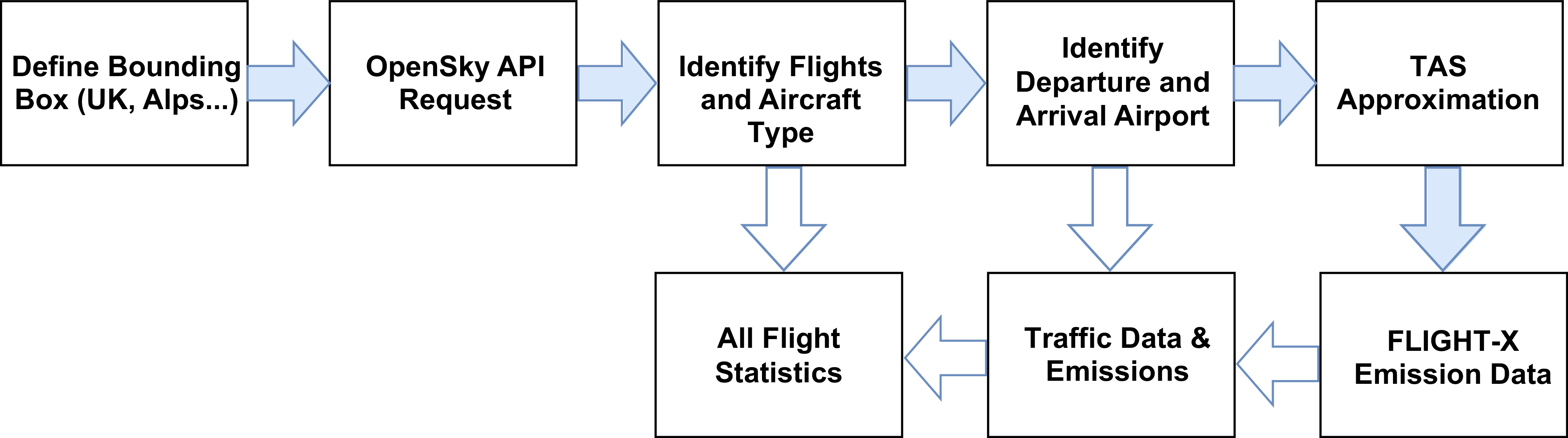
rely exclusively on modelling. Diversions and go-around regions that take into account international relations are not considered. A flowchart of the methods used is in Figure 1. First, a region is identified (by four corner coordinates, for simplicity); then, all traffic through the region is collected over a reference period (one week works best, but it can be seasonal). We have several databases: there is a meteorological database that allows us to estimate the true air speed from the ground speed (this is the only speed available on Automatic Dependent Surveillance - Broadcast (ADS-B) trajectories) and the air temperature.
Basic flowchart of the simulation methods used.

For a fixed region, we then have flight databases that consist of the following:
-
• A file containing a call sign, the hex-code, the aircraft type, the county of registration, and a pointer to the relative flight recording (from space-based ADS-B), that contains a time-stamp, an ICAO 24-bit identifier, latitude, longitude, ground speed and track angle, call sign, altitude and geo-altitude.
-
• On output file from FLIGHT-X that contains at least the following variables: IATA codes of origin/destination, date, ground temperatures at airfields, estimated take-off weight, distance flown, flight time, all emission species and more.
If needed, flights originating or terminating in any one point and passing through the box are identified. These databases are then used by another procedure to aggregate all statistics. A post-processing code, using the numerical methods described below, allows us to make a detailed estimate of what happens in the control box (see also results in the Appendix).
For the acoustic analysis, some high-altitude flights within the box over the northern United Kingdom were identified and the experimental procedure described in § 3.3. The signal is characterised as a long-duration humming high-altitude noise that is defined by the quantity LAeq, the equivalent sound level [12]. All the methods used make use of their own contributions [Reference Filippone13] and databases.
2.1 Overflight databases
For the identification of overflights, we use the traffic library [Reference Olive, Basora, Pöpper and Strohmeier14] to access data from the OpenSky Trino repository [Reference Schäfer, Strohmeier, Lenders, Martinovic and Wilhelm15]. Initially, we define a box that contains the area of interest. We query the OpenSky network to obtain all flights that have a latitude and longitude pairing that lies inside the box in a period of time (one day, one week, one month). For each flight identified, the minimum altitude is evaluated to determine whether the aircraft is operating solely in upper airspace (FL245 or above). If this is the case, the portion of the trajectory within the box is stored for further processing. Data may be affected by different time frequencies and incorrect altitude readings (NaN), which have to be removed. Flights with a small time of residence are removed from the database (20 s or less, corresponding to
 $\sim$
2.5 n-miles). For ease of simulation, all the geographical areas are defined by a quadrilateral delimited by a range of latitudes and longitudes.
Several characteristics can be detected, but they mostly require additional databases, real-time measures and observations. Origin and destination are not always available; these are critical to several observations and quantitative estimates, but there are ways around this difficulty with methods that have not been considered, but some comparisons are offered when these data are indeed available.
2.2 Flight simulation
Flight simulation is achieved by using the computer code Flight-X, described in Ref. [Reference Filippone13] and related publications. The performance modelling relies on separate modules for engine aero-thermodynamics, flight mechanics, configuration aerodynamics, propeller propulsion (if required), emissions and acoustics. Core to this approach is the underlying database, which consists of over 100 airplanes and engine models (commercial, freighters, turboprops, business, general aviation and military), limitations and other data extracted from the type certificate data sheets (TCDS). The model has been tested at all levels with available experimental data, flight data, commercial databases (for example, Ref. [Reference Filippone and Parkes16]) and some computer codes from other organisations that are widely used [Reference Mouillet17]. For the models that are not yet available, a table has been produced that maps non-existing airplanes to existing ones with various degrees of confidence (mostly business jets, which are delivered bespoke on an individual basis). The ICAO four-digit identification code has been used.
The solution requires an accurate estimate of the configuration drag at all flight conditions. For an aircraft in steady state, the aero thermodynamics of the engine is solved in inverse mode, where the speed
 $N1\%$
and fuel flow
 $W_{f6}$
are calculated from the estimated thrust.
2.2.1 Emissions modelling
The combustion emissions other than CO
 $_2$
are more problematic. Modelling fuel burn is easier than modelling the combustion chemistry in the general case, because too many parameters are unknown. To begin with, the ICAO publishes data on emission indices at four conventional points. LTO emissions are calculated according to the time-in-mode at each operational point, unlike the prescription from the ICAO reference durations and engine speeds. These operating points and their duration do not correspond to reality.
It is necessary to resort to a model of engine emissions that yields emission indices. Emission indices (CO, NO
 $_x$
, UHC, soot) from non regulated engines (turboprops, small turbofans with rating below 26.7 kN) are either found by a method described in Ref. [Reference Filippone and Bojdo18] or inferred from machine learning techniques whose benefits are being researched. All emissions are modelled and associated with tropospheric and stratospheric. The tropopause is by default 36,000 feet. We are aware of models that consider the troposphere at variable altitudes, both seasonal and geographical [Reference Mateus, Mendes and Pires19], but an attempt to judge a change in the results did not lead to a useful demonstrated result.
Emission indices measured at sea level, in specified atmospheric conditions [20], must be corrected for atmospheric effects (altitude, pressure, humidity), flight effects (Mach number or true air speed) and operational conditions (part throttle, or engine rpm or fuel flow fraction). One of the popular methods is the Boeing Fuel Flow Model, Version 2 (BBFM2), but it covers engines that are 40 or more years old and only a few of the emission species [Reference Baughcum, Tritz, Henderson and Pickett21]. There is a later method called P3T3 [Reference DuBois and Paynter22], which relies on `proprietary’ engine and airplane performance. In the present approach, we have all the parameters to conduct such analysis, e.g.
 $T_3$
(compressor exit temperature),
 $P_3$
(compressor exit pressure) and a host of other aero-thermodynamic quantities at every operational condition of the engine (temperature, altitude, Mach number and part throttle) – about two dozen, in fact. In the BFFM2, the flight Mach number correction depends on the factor
 $0.2 \, M^2$
. In this instance, there is no such correction, because all the aero-thermodynamic parameters are calculated at the corresponding Mach number. In other words, parameters such as
 $W_1$
are already corrected for Mach number or intake ram effects. Alternative methods for fuel flow have appeared in the technical literature since, for example Chati et al. [Reference Chati and Balakrishnan23], and most recently Poll et al. [Reference Poll and Schumann24]. These methods have not been implemented.
The emission of pollutants such as particulate matter, non-volatile particulate matter (nvPM) is calculated with the method called ImFOX of Reference [Reference Abrahamson, Zelina, Andac and Vander Wal25]. The volumetric flow rate is replaced by
 $W_1$
(air flow rate), but most likely this is
 $W2.5$
(core mass flow rate, since there is no combustion in the bypass). However, concentration of black carbon will depend on where the reference section is and how the particulate is collected. The temperature
 $T_4$
(combustor absolute temperature) is calculated exactly as in ImFOX, although the engine data include actual calculation of
 $T_4$
, which could be used. The fuel-to-air ratio is taken from the engine simulation rather than the values suggested by ImFOX. There will be some variability in results as a consequence, and differences with the original method and later First Order Approximation version 3 (FOA3) method [Reference Wayson, Fleming and Iovinelli26]. It has been demonstrated previously [Reference Filippone and Bojdo18] that at low engine rpm the approximation of the various methods depends critically on how the interpolating function is chosen among the ICAO reference points.
2.2.2 Assumptions and approximations
The origin and destination of the flights are generally not known. Therefore, it is not possible to make precise inferences about many aspects of the flights. The effect is compounded by the absence of critical data such as gross weight, passenger load, freighter load and weight and many other important parameters that are not known. An approach was proposed in Reference [Reference Filippone and Rotherham27]. Since then, the origin-destination pairing has become available, and re-analysis has revealed that inferences on distances and weight profile are not always accurate, though this is the only possibility in absence of critical data. The following discussion focuses on the overflights when origin and destination are known. For the case when they are not, refer to Reference [Reference Filippone and Rotherham27].
In the first place, the flight of the origin-destination pairing (for ex. EGLL-KJFK) waypoint in the reference box is calculated. The total distance flown is the sum between two great circle distances; this approximates the actual range.
The actual fuel burn
 $E_1$
and emissions
 $E_2$
are calculated from the flight distance within the region of interest, Figure 6, and two regression parameters
 $a$
and
 $b$
 \begin{eqnarray} E_1 = \frac {x_o}{x_1} \left ( a_i + b_i x_i \right ) \end{eqnarray}
 \begin{eqnarray} E_2 = \frac {x_o}{x_1} \left ( a_i + b_i x_i + c_i x^2 \right ) \end{eqnarray}
where
 $x_o$
is the length across the reference box and
 $x_1$
is the actual distance calculated previously;
 $x_o/x_1$
is the relative flight length within the box. The coefficients
 $a_i$
,
 $b_i$
,
 $c_i$
are calculated by appropriate least squares of the existing data.
For example, in the database, the A388 flies on average for 4,500 n-miles (
 $X_{max} =$
7,150 n-miles;
 $X_{min} =$
3,200 n-miles). If a flight over the region of interest is 94 n-miles, the corrected fraction of flight distance is
 $x_c = 94/4,500 = 0.020888$
.
In a previous simulation [Reference Filippone and Rotherham27], it was shown that a long-range passenger service with an A388 yields
 $\overline {X}_{min} = 2,516$
n-miles and
 $X_{max} = 7,558$
n-miles (OMDB to KLAX); from there, the most likely estimate of the average range was 6,046 n-miles; the corrected fraction of flight distance was
 $x_o/x_1 = 0.01555$
.
The law of large numbers compounds to our advantage, and in fact we found the following results for the A388: carbon-dioxide emissions when the origin-destination was unknown is
 $W_{CO2} =$
167.74 tons (old method); when the pairing is known,
 $W_{CO2} =$
163.67 tons (new method). Therefore, the difference is less than 2.5% of the original findings.
We are not so fortunate for shorter-range and business aircraft. In fact, the smaller the weight profile of the airplanes, the larger the difference between the old and new methods. For example, in the case of the Pilatus PC-12, the difference is
 $W_{CO2} =$
4.06 tons (old method),
 $W_{CO2} =$
1.73 tons (new method), leading to a difference which is over a factor of two. In this case, there is no alternative to retrieving the origin-destination pair to make a realistic analysis.
An example is shown in Figure 2 for the A350-900 (A359) as a function of the flight distance from space-based trajectory data. The minimum distance in this case is 250 n-miles, although shorter flights are done for operational reasons (these flights have been excluded from the analysis). The charts also show the difference between a linear regression and a quadratic one. The difference increases with larger flight distances, as a result of the aircraft having to tanker more fuel as the range is increased. Both mathematical approximations have been used to understand the role of the data modelling on the overall results. It is only beyond 6,000 n-miles that there are practical differences between the interpolation methods.
Once the ICAO code for a specific aircraft has been identified, fuel consumption and all emissions are correlated with the appropriate regression law, subject to a minimum distance being 150 n-miles (short), 200 n-miles (medium), 250 n-miles (long range), respectively. The shorter-range targets mostly domestic overflights or repositioning.
Fuel burn rates and NO
 $_x$
emissions from flights of the A350-900 (ICAO
 $=$
A359).

Fuel burn rates simulated for the Boeing B787-9 and the Pilatus PC-24.

2.2.3 Atmospheric data
Atmospheric data are sourced from the relevant Meteorological Aerodrome Report (METAR) stations in the region of interest to evaluate temperature, winds, cloud cover, all related to some aspect of emissions. The temperature is of no concern in the period analysed; the maximum range is noted as between 15–20 degrees Celsius in Northern England and Ireland, and lower and depending on the altitude in the Eastern Alps (Appendix C).
2.2.4 Sensitivity analysis
Numerical analysis conducted on least squares approximations, both linear and polynomial (Equations. 1 and 2) reveal a negligible difference in results, less than 2% on NO
 $_x$
emissions and
 ${\sim}3\%$
on the fuel burn, overall. Therefore, the use of polynomial regressions like the one shown in Figure 2 is not materially different from the linear approximation. Each circle is a simulated flight using the actual range.
Alternatively, we can use an average fuel burn expressed in fuel/available-seat/n-mile (FASM), which was previously calculated over a large number of flights. An example is given in Figure 3 for two different airplane classes. Graph 3a illustrates the performance of the Boeing B787-9 (a long-range commercial airliner); graph 3b shows the performance of a mid-range business jet, the Pilatus PC-24. There are two things to note. First, the FASM is relatively constant for each aircraft, providing the range is not too short. Second, there is a substantial difference in FASM between the two aircraft shown in Figure 3a: there is a factor 3.7:1 between the PC-24 and the B787-9 for the most common range (4,000 and 400 n-miles, respectively). For clarity, in the middle range, we expect a fuel burn rate of
 $\sim$
0.035 kg/seat/n-mile (
 $\sim$
2.25 lit/100 km) in the former case and
 $\sim$
0.16 kg/seat/n-mile (
 $\sim$
8.5 lit/seat/100 km) in the latter case, assuming an 8-seat configuration.
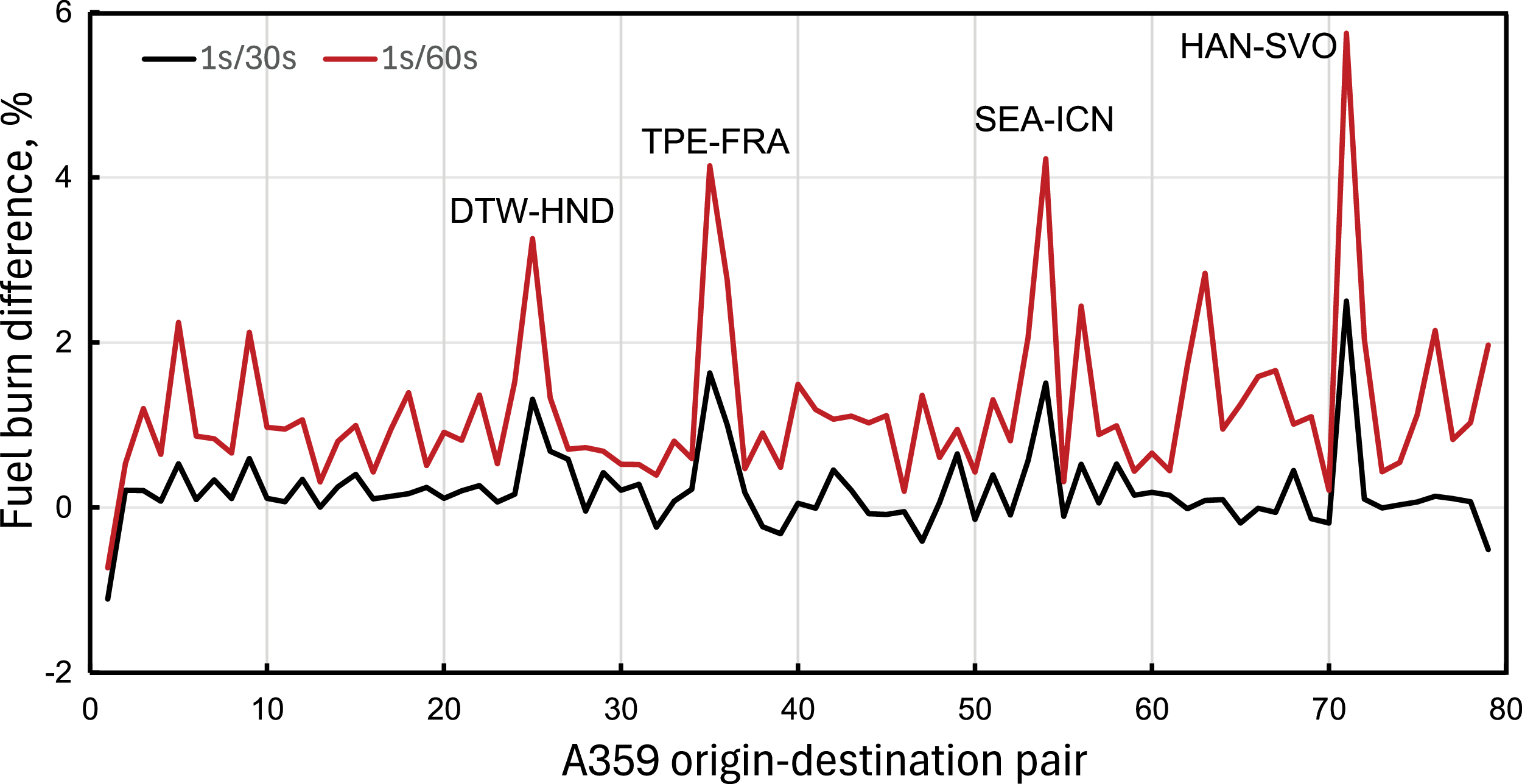
The trajectories used are in 1-second parsing. Analysis on coarser time steps of the A359, up to 1/60, reveals small changes in fuel burn, below 6% (Figure 4); the difference between the great-circle distance and actual distance is 5–10% for up to 80 distance-destination pairs. This aircraft carries out intercontinental service with an average of
 ${\sim}4,000$
n-miles (middle of Figure 2) but also some extremely long flights. Some origin-destination pairings are shown in Figure 4. The difference in estimated fuel burn is relatively modest, depending on the route and trajectory.
Sensitivity analysis on fuel burn rates from flights of the A359 with IATA codes.

2.2.5 Verification of results
Verification and validation are always a complicated matter due to the sparse availability of data that have been provided independently, and due to the long chain of calculations leading to a final result. It is necessary to establish the correct initial conditions, the actual taxi times, the gross take-off weight, the atmospheric conditions during the flight and particularly winds. Hence, we use default settings. There are too many parameters to mention, which depend on aircraft, route, passenger load, destination airfield, hold altitude, baggage allowance, diversion fuel and more. Outbound and inbound taxi times are considered constant, though there is indication that this is not the case in reality from data reported by Eurocontrol.
We use the EEA/EMEP Corinair Version 2023 [10] for the Airbus A320 Neo (A20N) and calculate the fuel burn and carbon dioxide CO
 $_2$
emissions for a flight range up to 3,000 n-miles, which is the range detected for 700 random flights. This is shown in Figure 5.
Comparison of fuel burn for the A320 Neo (A20N with Leap 1A engines) with the EEA/EMEP Corinair data [10] (dashed line).

Simulations have been carried out with and without LTO. Two cases were considered: (1) emissions above 24,500 feet, and (2) complete trajectories from wheel-up to wheel-down. It has been assessed that especially when the required range is short to medium, the overall flight must be considered to accurately capture the amount of emissions at altitude.
2.3 Input data
The input data consist of the following:
-
• A file containing the flight tracks, the corresponding hex-code, ICAO type code, registration, origin and destination, if available. Each of these flight tracks corresponds to airplanes that have been within the window examined for a minimum amount of time (Figure 6).
-
• Flight tracks of airplanes crossing the required window from ADS-B databases. Each file contains a time-stamp, ICAO24 of the airplane, latitude, longitude, ground speed, track angle, altitude and geo-altitude. The ground speed is replaced by the true air speed from the local wind speed and direction, if this is available from alternative databases, for example CAMS (Copernicus Atmosphere Monitoring Service).
-
• A worldwide database of fuel burn and emissions for a range of flights for each of the aircraft.
-
• A database of METAR atmospheric data at local airfields (if necessary).
3.0 Results and discussion
From the data and the simulation models, we can make both statistical inferences and quantitative estimates. We derive exact statistics of origin and destination points, flight patterns, network effects, weather conditions, CO
 $_2$
and non-CO
 $_2$
emissions.
3.1 Selecting region of interest
We consider first the case of Northern England, a region of extensive cruising traffic (i.e. traffic not using the local airports) at altitudes above 24,500 feet. Nearly 6,000 were detected overflights/week, or one flight every 90 s, on average. We estimate that there are about 1.25 million air passengers every week in those overflights who never touch the ground at local airports.
This number is presumably exceeded during the summer. In fact, the experiment was repeated for the first week of April and September 2025. The latter revealed an increase in the number of weekly flights by over 10% (6,593 overflights), mostly run by the same type of aircraft, 3% of which are business flights. The computational procedure is demonstrated for the latter week.
The region is at the crossroads for transatlantic East–West traffic. Flights from Amsterdam and Frankfurt bound for destinations all over North America cruise above Manchester, and vice versa. Flights from Los Angeles (ICAO = KLAX) and Tokyo Narita (RJTT), bound for London, Paris, Amsterdam and Frankfurt, cruise above Manchester. Flights to/from Dublin (EIDW) use Manchester (EGCC) as a waypoint at altitudes between 35,000 and 38,000 feet. Furthermore, there is North-South traffic, for example, from places such as Reykjavik, Iceland, destinations in Norway, traffic to/from other airports in the region, such as Manchester (EGCC), Liverpool (EGGP) and Leeds-Bradford (EGNM). There is the domestic North-South traffic to/from destinations in Scotland, plus holiday destinations to both the South-East and South-West.
An example of flight frequency is shown in Figure 6 for the box delimited by longitude [
 $-$
3:0] degrees and latitude [53.05: 53.93] degrees; the area covered is about 19,900 km
 $^2$
. The blue lines denote all overflights with an altitude above FL245. The red lines refer to flights that start above the threshold FL245 that at some point fall below, most likely for landing at one of the airports in the region or beyond. Likewise, they can cross the threshold of FL245 if they depart from one of those airports. Region A denotes the convergence of the trajectories are the start of the standard terminal arrival route (STAR) through a waypoint known as NUGRA for London Heathrow (EGLL). Region B is Manchester Airport (EGCC); zone C is the location of general aviation traffic performing circuits. Region B is the waypoint for air traffic from Dublin (EIDW).
One week of overflights above Northern England; the labels indicate coordinates in degrees.

The weekly frequency of flights indicates that over 18% occurs overnight (22:00-06:00 GMT), and peak traffic occurs in the morning, over 27%. The number is fairly stable over the days of the week, although it peaks on a Monday. UK registered carriers are
 $\sim$
37%; most of the traffic is international – either a pure overflight or an origin/destination with a UK airport. It is noted that some of these registrations are for fiscal convenience and include countries slightly more generous than the United Kingdom.
CO
 $_2$
, NO
 $_x$
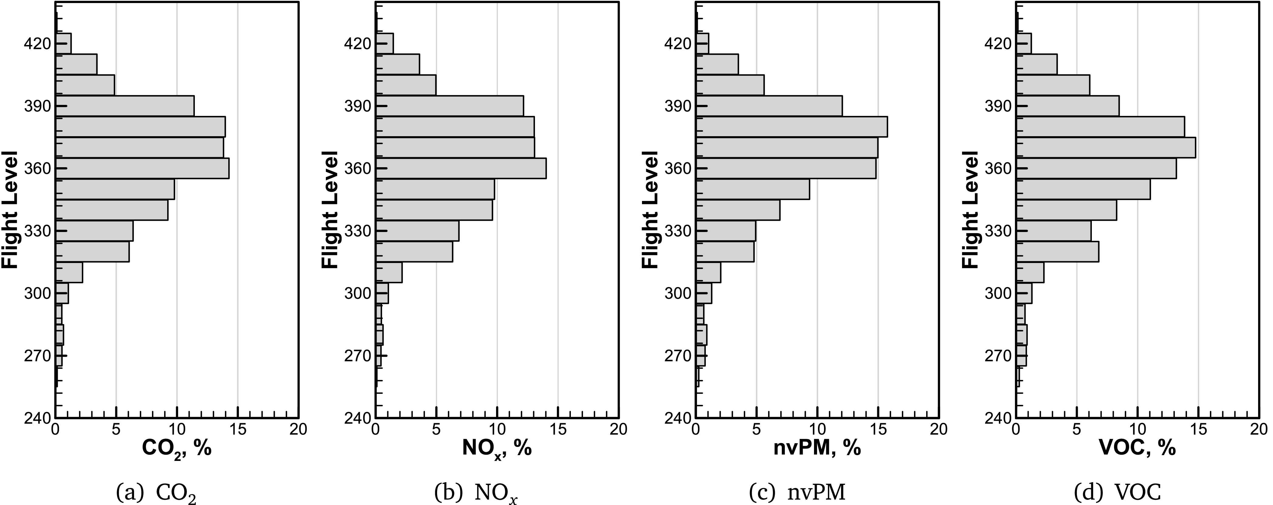
, nvPM, VOC emissions estimated from overflights in the region of Figure 6.

3.2 Estimating exhaust emissions
Output data from the computational chain can be organised in terms of altitude, duration, time of the day, aircraft family type and other characteristics.
Figure 7 shows a vertical distribution of fuel burn, NO
 $_x$
, non-volatile particulate matter (nvPM) and volatile organic compounds (VOC) emissions up to FL420 (42,000 feet). Only 40 flights (0.67%) are above this altitude, mostly long-range business flights (Gulfstream G650, and Global Challenger C600 Series). Similar analysis can be carried out for other emission species. The graph indicates that there is a substantial stratospheric portion (altitude
 $\gt$
36,000 feet) of the emissions within the window, and that there is a spread of emissions across the flight levels, due to the variety of aircraft flying over. Such a distribution can be demonstrated for each aircraft type. Similar results are obtained with other emission species, particularly uncombust hydrocarbons (UHC) and water vapour. In the appendix we provide a summary, Table B2. The effect of high-altitude NO
 $_x$
has been demonstrated previously as dependent on the region [Reference Maruhashi, Grewe, Frömming, Jöckel and Dedoussi28], and this can be quantified by looking at overflights in that region.
A stratospheric flight time is identified on 57% of the flights. The overflights cover over 377,000 n-miles (
 ${\sim}54$
n-miles each) within the box and burn
 ${\sim}3,000$
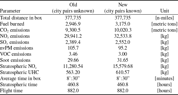
metric tons of jet fuel. On the vertical distribution of overflights, FL350 is the most popular with short- to medium-range aircraft, such as the A20N, A21N, A319, A320 and A321. About 5% of the overflights take place at FL400 or FL410. These are long-range intercontinental services with the A333, A35K, A388, B788 and B789 bypassing the UK airspace entirely. Overflights of the B38M, originating or landing in Ireland, operate in the same airspace at FL350 to FL410. When there are data on origin and destination, the estimates of emissions are straightforward, because it is possible to establish the length of the flight, the point at which emissions take place, even if the take-off weight is only approximate. The numerical methods remain valid in both cases; over the entire period analysed, the approximations tend to collapse.
In fact, over the entire week under inspection, within the same box, the difference in fuel burn goes down from
 $W_f =$
3,175 tons to
 $W_f =$
2,947 tons, a decrease of only about 7%, which is extraordinarily accurate considering the lack of flight data. A summary is provided in Table 1. Whilst the total flight distance could be captured in both cases, some flights could not be identified. Data specified as `stratospheric’ refer to emissions above 36,000 feet (FL360).
Emissions from overflights simulated in Northern England, one week in September 2025

Table 1. Long description
A table comparing emissions from overflights in Northern England for a week in September 2025. The table has 12 rows and 4 columns. The columns are labeled ‘Parameter’, ‘Old (city pairs unknown)’, ‘New (city pairs known)’, and ‘Unit’. The rows list various parameters and their corresponding values. Row 1: Total distance in box, 377,735, 377,735, [n-miles]. Row 2: Fuel burned, 2,946.9, 3,175.0, [metric tons]. Row 3: CO emissions, 9,300.5, 10,020.3, [metric tons]. Row 4: NO emissions, 29,941.2, 32,533.8, [kg]. Row 5: SO emissions, 2,389.4, 2,552.0, [kg]. Row 6: nvPM emissions, 105.7, 95.2, [kg]. Row 7: VOC emissions, 3.46, 3.00, [kg]. Row 8: Soot emissions, 29.66, 31.65, [kg]. Row 9: Stratospheric NO, 11,280.54, 15,579.68, [kg]. Row 10: Stratospheric UHC, 563.20, 610.57, [kg]. Row 11: Average time in box, 8:30, 8:30, [minutes]. Row 12: Stratospheric time, 460.8, 460.8, [hours]. Row 13: Flight time, 882.0, 882.0, [hours].
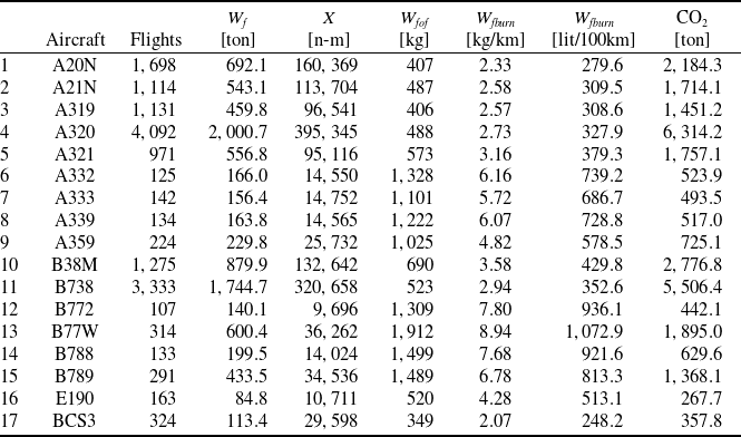
We expanded out analysis to the Eastern portion of the Alps, involving several countries (see Table C1 and Figure C1), where a number of flight fall below FL245.
3.3 Cruise noise
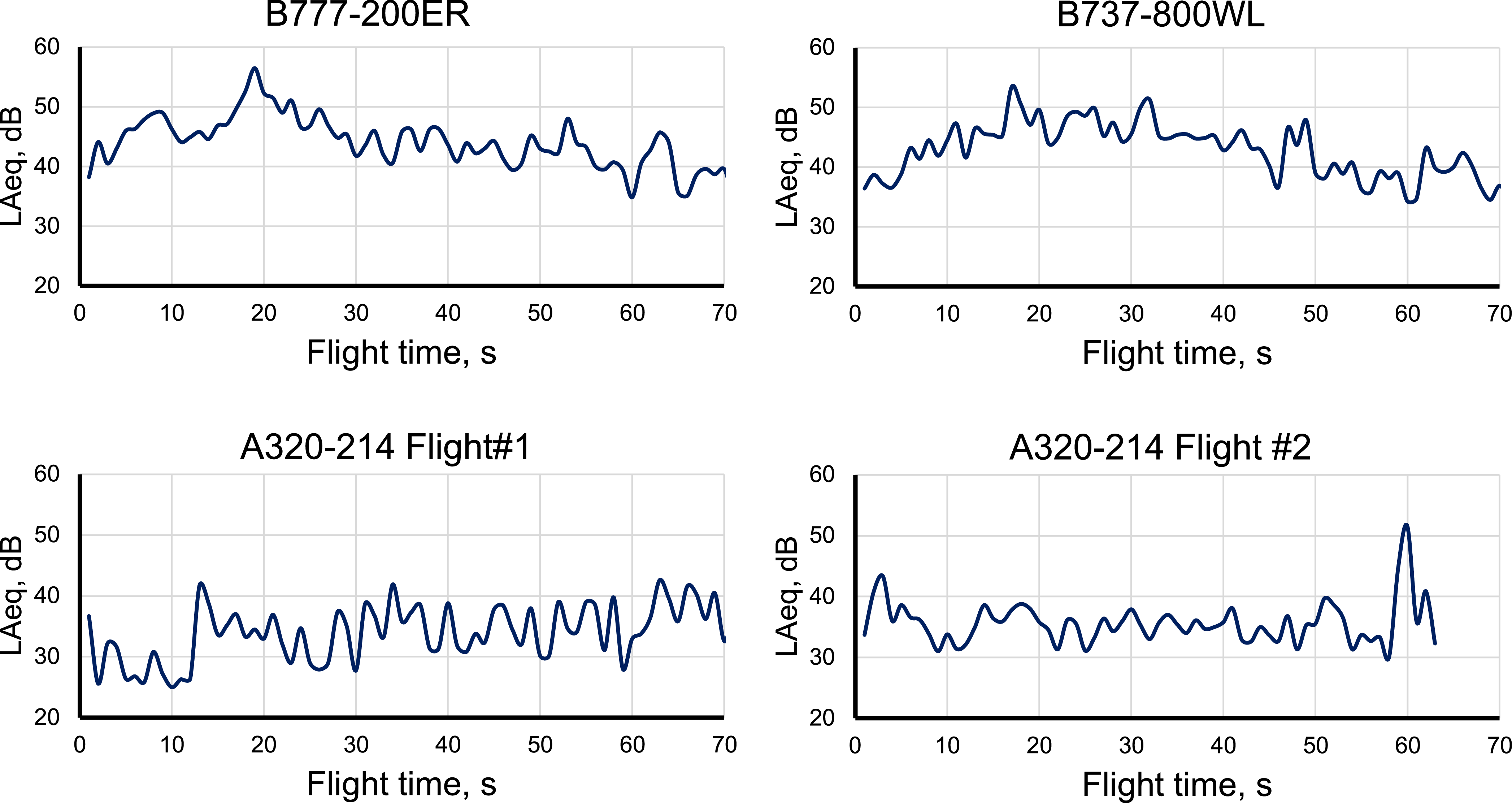
Other than large conurbations, where in some atmospheric conditions all airplanes can be heard, the countryside is affected by increasing levels of cruise noise. Airplanes at all altitudes can be heard and their noise measured. Unlike take-off and landing, high-altitude noise is characterised by long-lasting rumbles (2 or more minutes), with occasional peaks and silences due to the rapidly changing atmospheric conditions along the propagation front of the acoustic waves. An example is shown in Figure 8 where only a few airplanes are selected. The measurement was at a location called Colt Park (GPS position:
 $54.19498, -2.34999$
), with a B&K 2250 sound level meter. The sound meter was placed 4 feet (1.2 m) above the ground and acoustic signatures automatically recorded following standards set by ISO 20906 [29, 30]. Ground temperature on the day ranged between 2 and 5 °C. Noise is characterised by a maximum level and a duration above the background noise. There is no straightforward noise increase and decrease of the signal, as it is possible to see in low-level flight. The data stop at about 70 s and are all in tropospheric flight altitudes. Each flight has its own acoustic signature; even for the same aircraft there are notable differences, depending on flight level and atmospheric conditions – the latter ones critical to the acoustic propagation front. The A320 is a typical test case, as seen in Figure 8.
Selected measurements of cruise noise.

Figure 8. Long description
Panel A: A line graph titled B777-200ER shows the noise level in decibels (dB) on the vertical axis and flight time in seconds (s) on the horizontal axis. The noise level fluctuates between 30 and 50 dB over a 70-second flight time. Panel B: A line graph titled B737-800WL shows the noise level in decibels (dB) on the vertical axis and flight time in seconds (s) on the horizontal axis. The noise level fluctuates between 30 and 50 dB over a 70-second flight time. Panel C: A line graph titled A320-214 Flight #1 shows the noise level in decibels (dB) on the vertical axis and flight time in seconds (s) on the horizontal axis. The noise level fluctuates between 20 and 50 dB over a 70-second flight time. Panel D: A line graph titled A320-214 Flight #2 shows the noise level in decibels (dB) on the vertical axis and flight time in seconds (s) on the horizontal axis. The noise level fluctuates between 20 and 50 dB over a 70-second flight time.
The level of quietness, defined as being further away from any overflights, is shown in Figure 9. Light colours indicate quiet areas, although much depends on the minimum and maximum threshold values. Several tracks are present at the same time, which makes noise more detectable, though not attributable to a single source.
Frequency of overflights over Northern England.

4.0 Conclusions
High-altitude cruise flights affect several regions in the world. There is lack of regulation in this sector. Importance is currently given to international hubs of air traffic, where emissions are at low levels. The scenario is gradually degrading due to the increasing long-distance market demand and international route fragmentation. For the region analysed, overflights are about 7,000 per week, or
 $\sim$
1,000 per day, with a peak early in the week. Flights are concentrated in the altitude band FL330 to FL410. Further investigations can be carried out on flight frequency, location-dependent flight-hour density, lateral and vertical separation, etc. Finally, these emissions can be studied in terms of weeks, months or seasons.
We demonstrated a method for estimating the overall emissions, both CO
 $_2$
and non-CO
 $_2$
. Whilst the former can be compared with other existing methods, the actual values for all emissions can be found by direct measurement. The choice of a quadrilateral box facilitates the simulations. However, this contribution did not deal with long-term climatic effects.
Regarding noise, partial evidence indicates that the humming noise from cruising aircraft is above the background noise for about 2 minutes for every overflight. Background noise in the countryside averages 35–40 dBA, and peak cruise noise is 56–57 dBA, sometimes 70 dBA, depending on wind direction and flight altitude. This matter is left open for further investigation.
Acknowledgements
This research was part of the NERC-funded JetZero project at the University of Manchester (NERC APP 20794 – REVEAL-NOx, R131688, Non-CO
 $_2$
emissions from aviation). Land-based ADS-B data are open source. Space-based ADS-B data have been used thanks to a bilateral agreement with Aireon LLC. The origin-destination pairing was added thanks to the grateful help of Jannis Lübbe, from OpenSky. Research data and computer codes are made available upon reasonable request.
Appendix A. Sample results, Northern England
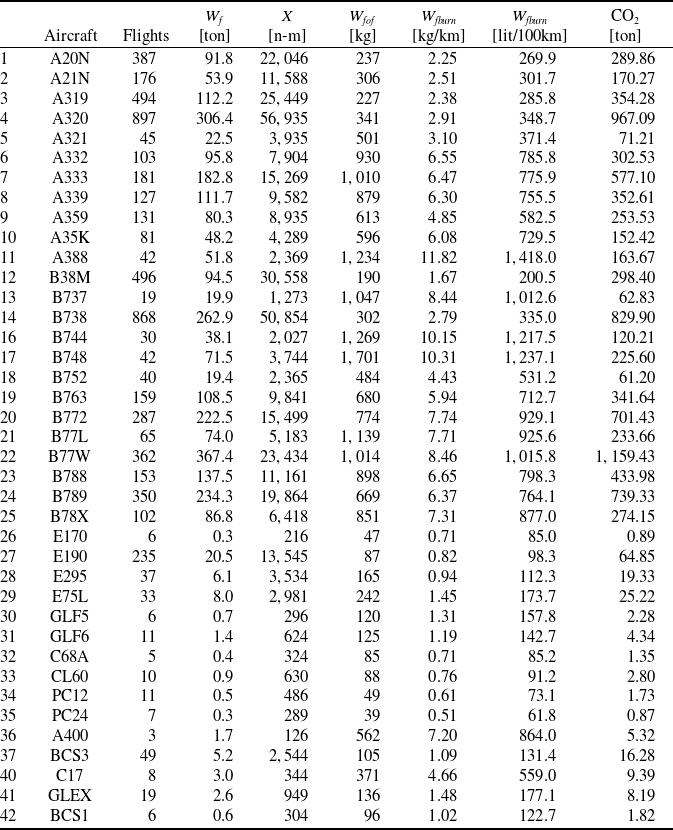
Below is a table of the aircraft identified and simulated through the computational chain described (ICAO 4-letter codes) in Northern England in one week of September 2025, Table B2. We have used the new method discussed in section 2.2. In the table,
 $W_f$
is the total fuel burn over the reference window;
 $W_{fof}$
is the estimated fuel burn during the overflight in the window of Figure 6;
 $X$
is the distance flown in the same region. Fuel burn rates,
 $W_{fburn}$
are also provided at the far right of the table. They represent about 94% of the flights detected. Missing aircraft were not identified. The table shows that the majority of flights are commercial; a minority is made up of cargo, business and military operations.
Database of overflights simulated

Table A1. Long description
The table presents data on different aircraft types, detailing their flights, fuel weight, and carbon dioxide emissions. It includes 42 rows and 8 columns. Column headers are Aircraft, Flights, Wf [ton], X [n-m], Wtof [kg], Wfburn [kg/km], Wfburn [lit/100km], and CO2 [ton]. Row labels include aircraft types such as A20N, A21N, A319, and others. Each row provides specific values for each column, showing the number of flights, fuel weight, distance in nautical miles, total fuel weight, fuel burn rate per kilometer, fuel burn rate per 100 kilometers, and carbon dioxide emissions in tons. Notable trends include variations in fuel burn rates and CO2 emissions across different aircraft types.
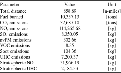
Estimated emission over Ireland; may include areas over the Atlantic ocean

Table B1. Long description
A table with 19 rows and 10 columns detailing estimated emissions over Ireland. The columns are labeled Parameter, Value, and Unit. The table includes data on total distance, fuel burned, and various emissions such as CO, NO, SO, nvPM, VOC, soot, UHC, stratospheric NO, and stratospheric UHC. Each row provides specific values for these parameters. For example, Row 1: Total distance, 858,89, n-miles; Fuel burned, 10,357.13, tons; CO emissions, 32,687.10, tons; NO emissions, 114,265.68, kg; SO emissions, 8,350.05, kg; nvPM emissions, 302.66, kg; VOC emissions, 8.35, kg; Soot emissions, 104.36, kg; UHC emissions, 7,200.37, kg; Stratospheric NO, 51,966.19, kg; Stratospheric UHC, 2,184.33, kg.
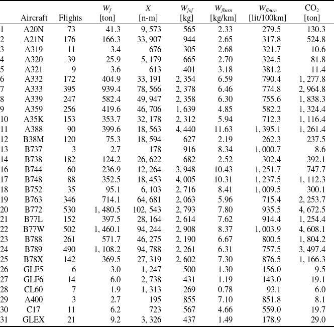
Database of overflights over Ireland

Table B2. Long description
The table compares different aircraft types based on several metrics. It has 31 rows and 9 columns. The columns are labeled Aircraft, Flights, Wf [ton], X [n-m], Wtof [kg], Wfburn [kg/km], Wfburn [lit/100km], and CO2 [ton]. Each row lists data for a specific aircraft type, including the number of flights, fuel weight in tons, distance in nautical miles, total fuel weight in kilograms, fuel burn rate in kilograms per kilometer, fuel burn per 100 kilometers in liters, and carbon dioxide emissions in tons. The table provides a detailed comparison of fuel efficiency and emissions for various aircraft.
Appendix B. Traffic patterns over Ireland
The numerical simulation procedure has been extended to other regions of the world. Figure B1 shows the traffic situation over the island of Ireland during the first week of September 2025. There is a clear East–West pattern. Most flights are overflights, with the exception of those descending or climbing FL245 at Dublin, Belfast, Cork (red traces). About 5,500 flights are in this chart, 69% of which fly at stratospheric altitudes. The reference box is bounded by LAT
 $= [ 51.5, 55.5]$
, LONG
 $= [ -11.0, -5.0]$
, and the number of passengers in these flights estimated at
 $\sim$
1.1 million/week. Regional jets, such as the Embraer 190 family, are represented in single-digit numbers. Flights of the A333 with origin-destination pairing show a total emission of 2,964.88 tons of CO
 $_2$
; without origin-destination, the result is 2,635.35 tons; therefore, in aggregate the difference is small. A summary is available on Table B1.
Overflight traffic pattern over the island of Ireland in September 2025.

Appendix C. Traffic patterns over Eastern Alps
As a final case, we show in Figure C1 the case of the Eastern Alps during one week in 2025. In this case, although there is clear North-South traffic across the continental divide, many flights descend or climb above FL245 to operate services at local airports, Milan or Bergamo in particular (ICAO
 $=$
LIMC or LIME). The reference region is within the coordinates LAT
 $=$
[44.0, 47.0], LONG
 $=$
[6.0, 12.0]. We estimate that there are about 3.5 million passengers/week in these overflights. Three silent air spaces can be found on the map. About 18,000 flights are in this chart. For this case, origin and destinations are unknown; the calculations were done without such information, unlike the previous cases. The most common flights are listed in Table C1, with their relative fuel burn.
List of the most common airplanes cruising above the Alps

Table C1. Long description
A table comparing various aircraft types based on their flight data and environmental impact. The table has 17 rows and 8 columns. Column headers are Aircraft, Flights, Wf [ton], X [n-m], Wf tot [kg], Wf burn [kg/km], Wf burn [lit/100km], and CO2 [ton]. Row 1: A20N, 1698, 692.1, 160369, 407, 2.33, 279.6, 2184.3. Row 2: A21N, 1114, 543.1, 113704, 487, 2.58, 309.5, 1714.1. Row 3: A319, 1131, 459.8, 96541, 406, 2.57, 308.6, 1451.2. Row 4: A320, 4092, 2000.7, 395345, 488, 2.73, 327.9, 6314.2. Row 5: A321, 971, 556.8, 95116, 573, 3.16, 379.3, 1757.1. Row 6: A332, 125, 166.0, 14550, 1328, 6.16, 739.2, 523.9. Row 7: A333, 142, 156.4, 14752, 1101, 5.72, 686.7, 493.5. Row 8: A339, 134, 163.8, 14565, 1222, 6.07, 728.8, 517.0. Row 9: A359, 224, 229.8, 25732, 1025, 4.82, 578.5, 725.1. Row 10: B38M, 1275, 879.9, 132642, 690, 3.58, 429.8, 2776.8. Row 11: B738, 3333, 1744.7, 320658, 523, 2.94, 352.6, 5506.4. Row 12: B772, 107, 140.1, 9696, 1309, 7.80, 936.1, 442.1. Row 13: B77W, 314, 600.4, 36262, 1912, 8.94, 1072.9, 1895.0. Row 14: B788, 133, 199.5, 14024, 1499, 7.68, 921.6, 629.6. Row 15: B789, 291, 433.5, 34536, 1489, 6.78, 813.3, 1368.1. Row 16: E190, 163, 84.8, 10711, 520, 4.28, 513.1, 267.7. Row 17: BCS3, 324, 113.4, 29598, 349, 2.07, 248.2, 357.8.
Overflight traffic pattern over the Eastern Alps in April 2025.



 x
 =



 2
 x




 Open access

