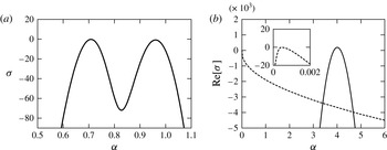
1. Introduction
Around a hundred years ago, Lord Rayleigh claimed a stability criterion for rotating shear flows by a simple physical intuition: the flow is stable if angular momentum increases outwards from the axis of rotation (Rayleigh Reference Rayleigh1917). However, contrary to the results of this model, the presence of turbulence in Rayleigh-stable flow is indirectly supported by observations in certain astrophysical flows, such as flow in accretion disks, for example. The existence of protoplanetary disks, whose ionisation is too weak for the observed turbulence to be explained by a magnetic mechanism, suggests that a purely hydrodynamic effect destabilises such Rayleigh-stable astrophysical flows. To examine this argument, Taylor–Couette flow, i.e. viscous flow between differentially rotating coaxial cylinders, has been examined intensively. Taylor (Reference Taylor1923) showed that the linear stability boundary of this flow asymptotes to Rayleigh’s result when the shear is large. In fact, for Taylor–Couette flow, Rayleigh’s criterion coincides with the inviscid limit of the linear stability to axisymmetric perturbations. Rich pattern formation phenomena, including a longitudinal vortex pattern, called Taylor vortex (TV) flow, have been observed when the flow is Rayleigh unstable. In contrast, despite decades of research, the question of the existence of sustained turbulence for Rayleigh-stable flows remains open. The most recent experiments on this phenomenon (Ji et al. Reference Ji, Burin, Schartman and Goodman2006; Paoletti & Lathrop Reference Paoletti and Lathrop2011) drew contrary conclusions to each other. The origin of the experimental difficulty is the unavoidable Ekman effect caused by the caps at the cylinder ends. Despite some sophisticated treatments of the endcaps in these experiments, Avila (Reference Avila2012) showed that the tiny Ekman effect is in fact non-negligible. As these experiments and numerical results suggest, the stability of Rayleigh-stable Taylor–Couette flow is dramatically affected by a small amount of cross-flow.
This sensitivity of the stability to the cross-flow simultaneously implies that, if the accretion effect is accounted for in Taylor–Couette flow by a radial cross-flow, the modelling of the Rayleigh-stable accretion disk instability could be improved. The radial cross-flow can also be found in rotating flows in our daily lives, e.g. bathtub vortex, tornadoes and the Earth’s polar vortex. Recently, Gallet, Doering & Spiegel (Reference Gallet, Doering and Spiegel2010, referred to as GDS10 hereinafter) imposed radial inward suction to Taylor–Couette flow, expecting that this additional accretion would destabilise rotational flows. Restricting attention to the stationary inner cylinder case, which is neutral according to Rayleigh’s stability criterion, they found linear instability to transverse rolls. Although this model (also considered earlier in Dubrulle et al. (Reference Dubrulle, Dauchot, Daviaud, Longaretti, Richard and Zahn2005)) is too simplified to apply directly to accretion disks, the result suggests that there is a different type of fluid instability other than the TV mode when the effects of shear, rotation and suction compete.
Our motivation is to present a broad overview of such instabilities by considering GDS10’s modelling as a canonical flow that describes a universal instability mechanism for swirling fluid motion. In the present paper, we further simplify the model to a flow between parallel plates taking the narrow gap limit. This reduction allows us to investigate a wider parameter region with some asymptotic reductions, and is likely to reveal the existence of the transverse-roll-type instability found by GDS10 in the Rayleigh-stable parameter range that would be relevant to astrophysical and geophysical applications. We also expect that this investigation will reveal the relation between the transverse-roll-type destabilisation and the earlier work by Min & Lueptow (Reference Min and Lueptow1994), where the stabilising effect of suction on the TV mode was shown.
In the shear-flow transition community, the effect of wall suction attracts attention as one of the accessible means to laminar–turbulent flow control. Various types of suction have been applied to several canonical shear flows. For example, boundary-layer flow control by discrete suction orifices at the wall has been discussed by Messing & Kloker (Reference Messing and Kloker2010). Of particular relevance to our model are the studies by Hains (Reference Hains1971), Sheppard (Reference Sheppard1972), Nicoud & Angilella (Reference Nicoud and Angilella1997), Fransson & Alfredsson (Reference Fransson and Alfredsson2003b ) and Guha & Frigaard (Reference Guha and Frigaard2010), where plane Poiseuille and/or Couette flows are considered with uniform wall suction. The motivations of these studies have come from not only flow control but also boundary-layer flow studies, since the basic flow is deformed sharply near the suction wall. We will show that our model also has a close connection to an external flow over a flat plate with uniform suction, referred to as the asymptotic suction boundary-layer flow (Hocking Reference Hocking1975; Milinazzo & Saffman Reference Milinazzo and Saffman1985; Fransson & Alfredsson Reference Fransson and Alfredsson2003a ; Khapko et al. Reference Khapko, Kreilos, Schlatter, Duguet, Eckhardt and Henningson2013; Deguchi & Hall Reference Deguchi and Hall2014).
The outline of the paper is as follows. In § 2, we begin by presenting the mathematical formulation of the problem. Section 3 concerns the linear stability analysis of the full Navier–Stokes problem in the wide range of parameter space. To describe the asymptotic behaviour of the linear neutral curves, several reduced problems are derived in § 4 by taking asymptotic limits of the governing equations. In § 5, the reduced problems are solved and compared to the results in § 3. Section 6 briefly investigates the possibilities of subcritical transition from the basic flow by examining finite-amplitude equilibrium solutions bifurcating from the linear instabilities. Finally, in § 7, we summarise our results.
2. Formulation of the problem
We consider a viscous incompressible fluid flow with kinematic viscosity
 ${\it\nu}^{\ast }$
and density
 ${\it\rho}^{\ast }$
between two coaxial cylinders. In cylindrical coordinates
 $[r^{\ast },{\it\theta}^{\ast },z^{\ast }]$
, the fluid is driven by inner and outer cylinders at
 $r=r_{i}^{\ast }$
and
 $r=r_{o}^{\ast }$
rotating with angular speeds of
 ${\it\Omega}_{i}^{\ast }$
and
 ${\it\Omega}_{o}^{\ast }$
, respectively. The cylinders also induce radially inward mass transport. If uniform suction with a speed of
 $-V^{\ast }$
is applied at the inner wall, there must be uniform injection with a speed of
 $-V^{\ast }r_{o}^{\ast }/r_{i}^{\ast }$
at the outer wall for the sake of mass conservation. There are two characteristic length scales in the problem: the mean radius
 $r_{m}^{\ast }=(r_{o}^{\ast }+r_{i}^{\ast })/2$
and the half gap
 $d^{\ast }=(r_{o}^{\ast }-r_{i}^{\ast })/2$
.
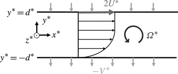
Sketch of the flow configuration.

Switching from the cylindrical coordinates to the gap coordinates
 $[x^{\ast },y^{\ast },z^{\ast }]=[r_{m}^{\ast }({\it\theta}^{\ast }-{\it\Omega}_{i}^{\ast }t),r^{\ast }-r_{m}^{\ast },z^{\ast }]$
and taking the narrow-gap limit
 $r_{i}^{\ast }/r_{o}^{\ast }\rightarrow 1$
, we can reduce the problem to a flow between parallel plates placed at
 $y^{\ast }=\pm d^{\ast }$
in Cartesian coordinates
 $[x^{\ast },y^{\ast },z^{\ast }]$
as depicted in figure 1. Note that a Galilean transformation in
 $x^{\ast }$
can be used to fix the lower wall speed to be zero. The fluid experiences shear and Coriolis forces due to the movement of the upper wall with a speed of
 $r_{o}^{\ast }{\it\Omega}_{o}^{\ast }-r_{i}^{\ast }{\it\Omega}_{i}^{\ast }=2U^{\ast }$
in the
 $x^{\ast }$
direction relative to the stationary lower wall and the rotation of the whole system with an angular speed of
 $({\it\Omega}_{i}^{\ast }+{\it\Omega}_{o}^{\ast })/2={\it\Omega}^{\ast }$
in the
 $z^{\ast }$
direction. The uniform background cross-flow with a speed of
 $-V^{\ast }$
is realised by the injection at the upper wall and suction at the lower wall. Taking the length, time and density scales as
 $d^{\ast }$
,
 $d^{\ast 2}/{\it\nu}^{\ast }$
and
 ${\it\rho}^{\ast }$
, we find that the non-dimensional total velocity
 $\boldsymbol{u}_{t}=u_{t}\boldsymbol{e}_{x}+v_{t}\boldsymbol{e}_{y}+w_{t}\boldsymbol{e}_{z}$
and generalised pressure
 $p_{t}$
, which includes the centrifugal effect, satisfy the Navier–Stokes equations
 $$\begin{eqnarray}\displaystyle & \displaystyle \frac{\partial \boldsymbol{u}_{t}}{\partial t}+(\boldsymbol{u}_{t}\boldsymbol{\cdot }\boldsymbol{{\rm\nabla}})\boldsymbol{u}_{t}=-\boldsymbol{{\rm\nabla}}p_{t}+{\rm\Delta}\boldsymbol{u}_{t}-{\it\Omega}\boldsymbol{e}_{z}\times \boldsymbol{u}_{t}, & \displaystyle\end{eqnarray}$$
 $$\begin{eqnarray}\displaystyle & \displaystyle \boldsymbol{{\rm\nabla}}\boldsymbol{\cdot }\boldsymbol{u}_{t}=0, & \displaystyle\end{eqnarray}$$
 $$\begin{eqnarray}\displaystyle \boldsymbol{u}_{t}=2R\boldsymbol{e}_{x}-S\boldsymbol{e}_{y} & \quad & \displaystyle \text{at}\ y=1,\end{eqnarray}$$
 $$\begin{eqnarray}\displaystyle \boldsymbol{u}_{t}=-S\boldsymbol{e}_{y} & \quad & \displaystyle \text{at}\ y=-1,\end{eqnarray}$$
 ${\rm\Delta}$
is the Laplace operator
 $\partial _{xx}^{2}+\partial _{yy}^{2}+\partial _{zz}^{2}$
and
 $\boldsymbol{e}_{x}$
,
 $\boldsymbol{e}_{y}$
and
 $\boldsymbol{e}_{z}$
are the unit vectors pointing in the
 $x$
,
 $y$
and
 $z$
directions, respectively. In (2.1)–(2.4), the parameters
 $R=U^{\ast }d^{\ast }/{\it\nu}^{\ast }$
,
 ${\it\Omega}=2{\it\Omega}^{\ast }d^{\ast 2}/{\it\nu}^{\ast }$
and
 $S=V^{\ast }d^{\ast }/{\it\nu}^{\ast }$
represent the effects of shear, rotation and suction, respectively. In the following, we mainly focus on the anticyclonic parameter region
 $R{\it\Omega}>0$
, which includes the Keplerian flow
 ${\it\Omega}={\textstyle \frac{2}{3}}R$
associated with celestial rotating systems. Notice that for the wide-gap cylindrical case the Keplerian motion is only realised at certain
 $r$
(called quasi-Keplerian flow). The symmetry of the system allows us to consider only positive
 $R,\ {\it\Omega}$
and
 $S$
.
In order to find the basic state, we substitute
 $\boldsymbol{u}_{t}=u_{b}(y)\boldsymbol{e}_{x}-S\boldsymbol{e}_{y}$
and
 $p_{t}={\it\Pi}x+p_{b}(y)$
into (2.1), to obtain
 $$\begin{eqnarray}-Su_{b}^{\prime }={\it\Pi}+u_{b}^{\prime \prime }-S{\it\Omega},\end{eqnarray}$$
where prime denotes differentiation with respect to
 $y$
and
 ${\it\Pi}$
represents the non-dimensional constant pressure gradient in the streamwise direction
 $x$
. We assume
 ${\it\Pi}=0$
so that the problem is consistent with the original cylindrical case, where the constant azimuthal pressure gradient must be absent. The basic flow, which is an exact solution,
 $$\begin{eqnarray}u_{b}(y)={\it\Omega}(1+y)+2(R-{\it\Omega})\frac{1-\text{e}^{-S(1+y)}}{1-\text{e}^{-2S}},\end{eqnarray}$$
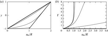
of (2.5), is plotted as the thin solid lines in figure 2(a,b) for
 $S=0.4,\ 4$
and 40 (to draw the figure we set
 ${\it\Omega}=R/2$
).
The basic flow profile
 $u_{b}$
for
 ${\it\Omega}=R/2$
as a function of (a) non-scaled vertical coordinate
 $y$
and (b) scaled vertical coordinate
 $Y=S(1+y)$
. The thick solid and dashed lines represent the profiles for
 $S=0$
and
 $S=\infty$
. The three thin lines are the profiles for
 $S=0.4$
, 4 and 40 (top to bottom for panel (a) and bottom to top for panel (b)).

For small suction (
 $S\ll 1$
) the basic flow (2.6) can be expanded as
 $$\begin{eqnarray}u_{b}(y)=R(1+y)+\frac{(R-{\it\Omega})}{2}S(1-y^{2})+O(S^{2}),\end{eqnarray}$$
and therefore behaves like rotating plane Poiseuille–Couette flow, which has the basic flow profile given by
 $u_{b}(y)=R_{PCF}(1+y)+R_{PPF}(1-y^{2})$
. When
 $S=0$
the basic flow becomes a linear profile, denoted by the thick solid line in figure 2(a).
When the limit
 $S\rightarrow \infty$
in (2.6) is taken, we find the fluid motion
 $$\begin{eqnarray}u_{b}(y)={\it\Omega}(1+y)+2(R-{\it\Omega})\end{eqnarray}$$
for
 $(1+y)\sim O(1)$
(the thick dashed line in figure 2
a) and the basic asymptotic suction boundary-layer profile,
 $$\begin{eqnarray}u_{b}(Y)=2(R-{\it\Omega})(1-\text{e}^{-Y}),\end{eqnarray}$$
for
 $Y=S(1+y)\sim O(1)$
(the thick dashed line in figure 2
b). The former equation (2.8) can be regarded as an inviscid core with a constant gradient
 ${\it\Omega}$
, whilst the latter equation (2.9), with a wall boundary-layer profile, controlled by the combined parameter
 $D\equiv R-{\it\Omega}$
, sharply modifies the overall flow to satisfy the no-slip conditions. This property allows the governing equations to have several interesting asymptotic limits, as we shall discuss in § 4.
When Rayleigh’s theory based on angular momentum distribution is extended to our model, the stability condition can be written as
 $u_{b}^{\prime }-{\it\Omega}<0$
and therefore, if
 $0<{\it\Omega}$
and
 $R<{\it\Omega}$
, the flow is Rayleigh stable for any value of
 $S$
. In the
 ${\it\Omega}{-}R$
parameter plane the Rayleigh-stable region is bounded by
 ${\it\Omega}=0$
and by
 $R={\it\Omega}$
, called the Rayleigh line. In the narrow-gap limit, the former stability boundary corresponds to the Rayleigh-neutral case studied by GDS10, where the inner cylinder is at rest. When the suction rate
 $S$
is zero, the system reduces to rotating plane Couette flow with the wall-shear Reynolds number
 $R$
and the rotation number
 ${\it\Omega}$
(Nagata Reference Nagata1986). In that case, it is known that Rayleigh’s stability criterion is a necessary condition for the inviscid linear stability criterion. However, we shall show that this is not true when suction is applied.
Subtracting the basic flow from the total field, we find that the disturbance velocity and pressure,
 $[u,v,w,p]=[u_{t}-u_{b},v_{t}-S,w_{t},p_{t}]$
, satisfy
 $$\begin{eqnarray}\left.\begin{array}{@{}c@{}}\{\partial _{t}+(u_{b}+u)\partial _{x}+(v-S)\partial _{y}+w\partial _{z}\}u+(u_{b}^{\prime }-{\it\Omega})v=-\partial _{x}p+{\rm\Delta}u,\\ \{\partial _{t}+(u_{b}+u)\partial _{x}+(v-S)\partial _{y}+w\partial _{z}\}v+{\it\Omega}u=-\partial _{y}p+{\rm\Delta}v,\\ \{\partial _{t}+(u_{b}+u)\partial _{x}+(v-S)\partial _{y}+w\partial _{z}\}w=-\partial _{z}p+{\rm\Delta}w,\\ \partial _{x}u+\partial _{y}v+\partial _{z}w=0,\end{array}\right\}\end{eqnarray}$$
together with the no-slip conditions
 $\boldsymbol{u}=0$
at
 $y=\pm 1$
. When the total flow is streamwise independent, the above equations reduce to
 $$\begin{eqnarray}\left.\begin{array}{@{}c@{}}\{\partial _{t}+(v-S)\partial _{y}+w\partial _{z}\}({\it\Omega}u)+{\it\tau}F_{B}v=(\partial _{yy}^{2}+\partial _{zz}^{2})({\it\Omega}u),\\ \{\partial _{t}+(v-S)\partial _{y}+w\partial _{z}\}v+({\it\Omega}u)=-\partial _{y}p+(\partial _{yy}^{2}+\partial _{zz}^{2})v,\\ \{\partial _{t}+(v-S)\partial _{y}+w\partial _{z}\}w=-\partial _{z}p+(\partial _{yy}^{2}+\partial _{zz}^{2})w,\\ \partial _{y}v+\partial _{z}w=0,\end{array}\right\}\end{eqnarray}$$
where
 $F_{B}(y)=-2S\,\text{e}^{-S(1+y)}/(1-\text{e}^{-2S})$
and
 ${\it\tau}={\it\Omega}(R-{\it\Omega})$
. Therefore, the system is governed only by Taylor number
 ${\it\tau}$
and
 $S$
. On the other hand, if the total flow is spanwise independent, the effect of system rotation
 ${\it\Omega}$
only appears in the basic flow (2.6); the reduced system in this case is
 $$\begin{eqnarray}\left.\begin{array}{@{}c@{}}\{\partial _{t}+(u_{b}+\partial _{y}{\it\varphi})\partial _{x}-(S+\partial _{x}{\it\varphi})\partial _{y}-(\partial _{xx}^{2}+\partial _{yy}^{2})\}{\it\varphi}-u_{b}^{\prime \prime }\partial _{x}{\it\varphi}=0,\\ w=0,\quad u=\partial _{y}{\it\varphi},\quad v=-\partial _{x}{\it\varphi},\end{array}\right\}\end{eqnarray}$$
where
 ${\it\varphi}$
is a stream function. This problem is essentially identical to non-rotating plane Poiseuille–Couette flow with uniform suction since the Coriolis force
 $S{\it\Omega}$
in (2.5) has the same effect as the pressure gradient
 ${\it\Pi}$
. The small-
 $S$
basic flow behaviour (2.7) similar to plane Poiseuille–Couette flow without suction is a special case of this analogy.
For numerical purposes, it is convenient to rewrite (2.10) in terms of potentials and mean-flow distortions. Assuming all physical quantities are periodic in the
 $x$
and
 $z$
directions with wavenumbers
 ${\it\alpha}$
and
 ${\it\beta}$
, respectively, the disturbance velocity is decomposed as
 $$\begin{eqnarray}\boldsymbol{u}=\overline{\boldsymbol{u}}+\tilde{\boldsymbol{u}}=\overline{u}\boldsymbol{e}_{x}+\overline{w}\boldsymbol{e}_{z}+\boldsymbol{{\rm\nabla}}\times \boldsymbol{{\rm\nabla}}\times ({\it\phi}\boldsymbol{e}_{y})+\boldsymbol{{\rm\nabla}}\times ({\it\psi}\boldsymbol{e}_{y}),\end{eqnarray}$$
where the mean-flow distortions are defined by the
 $x{-}z$
average operator
 $$\begin{eqnarray}\overline{\ast }=\frac{{\it\alpha}{\it\beta}}{4{\rm\pi}^{2}}\int _{0}^{2{\rm\pi}/{\it\alpha}}\!\int _{0}^{2{\rm\pi}/{\it\beta}}\ast \,\text{d}x\text{d}z.\end{eqnarray}$$
The equations for the potentials and mean-flow distortions can be found by operating
 $\boldsymbol{e}_{y}\boldsymbol{\cdot }\boldsymbol{{\rm\nabla}}\times \boldsymbol{{\rm\nabla}}\times \ast$
,
 $\boldsymbol{e}_{y}\boldsymbol{\cdot }\boldsymbol{{\rm\nabla}}\times \ast$
,
 $\boldsymbol{e}_{x}\boldsymbol{\cdot }\overline{\ast }$
and
 $\boldsymbol{e}_{z}\boldsymbol{\cdot }\overline{\ast }$
on the momentum equations in (2.10):
 $$\begin{eqnarray}\displaystyle \partial _{t}{\rm\Delta}{\rm\Delta}_{2}{\it\phi} & = & \displaystyle -((\overline{u}_{t}\partial _{x}-S\partial _{y}+\overline{w}\partial _{z}-{\rm\Delta}){\rm\Delta}-\overline{u}_{t}^{\prime \prime }\partial _{x}-\overline{w}^{\prime \prime }\partial _{z}){\rm\Delta}_{2}{\it\phi}\nonumber\\ \displaystyle & & \displaystyle -\,{\it\Omega}\partial _{z}{\rm\Delta}_{2}{\it\psi}-\boldsymbol{e}_{y}\boldsymbol{\cdot }\boldsymbol{{\rm\nabla}}\times \boldsymbol{{\rm\nabla}}\times ((\tilde{\boldsymbol{u}}\boldsymbol{\cdot }\boldsymbol{{\rm\nabla}})\tilde{\boldsymbol{u}}),\end{eqnarray}$$
 $$\begin{eqnarray}\displaystyle \partial _{t}{\rm\Delta}_{2}{\it\psi} & = & \displaystyle -(\overline{u}_{t}\partial _{x}-S\partial _{y}+\overline{w}\partial _{z}-{\rm\Delta}){\rm\Delta}_{2}{\it\psi}\nonumber\\ \displaystyle & & \displaystyle +\,(({\it\Omega}-\overline{u}_{t}^{\prime })\partial _{z}+\overline{w}^{\prime }\partial _{x}){\rm\Delta}_{2}{\it\phi}+\boldsymbol{e}_{y}\boldsymbol{\cdot }\boldsymbol{{\rm\nabla}}\times ((\tilde{\boldsymbol{u}}\boldsymbol{\cdot }\boldsymbol{{\rm\nabla}})\tilde{\boldsymbol{u}})=0,\end{eqnarray}$$
 $$\begin{eqnarray}\displaystyle \partial _{t}\overline{u} & = & \displaystyle \overline{u}^{\prime \prime }+S\overline{u}^{\prime }+\partial _{y}\,\overline{(\partial _{xy}^{2}{\it\phi}-\partial _{z}{\it\psi})({\rm\Delta}_{2}{\it\phi})},\end{eqnarray}$$
 $$\begin{eqnarray}\displaystyle \partial _{t}\overline{w} & = & \displaystyle \overline{w}^{\prime \prime }+S\overline{w}^{\prime }+\partial _{y}\,\overline{(\partial _{yz}^{2}{\it\phi}+\partial _{x}{\it\psi})({\rm\Delta}_{2}{\it\phi})},\end{eqnarray}$$
 ${\rm\Delta}_{2}=\partial _{xx}^{2}+\partial _{zz}^{2}$
and
 $\overline{u}_{t}=u_{b}+\overline{u}$
. The no-slip conditions on the walls become
 $$\begin{eqnarray}{\it\phi}=\partial _{y}{\it\phi}={\it\psi}=\overline{u}=\overline{w}=0\quad \text{at}\ y=\pm 1.\end{eqnarray}$$
3. The linear stability analysis
3.1. Numerical method
When disturbances are infinitesimally small, nonlinearity plays no role in the governing equations. In this case mean-flow distortions
 $\overline{u}$
and
 $\overline{w}$
are negligible and the potentials can be written as the sum of normal modes:
 $$\begin{eqnarray}\displaystyle {\it\phi}(x,y,z,t) & = & \displaystyle \exp (\text{i}{\it\alpha}x+\text{i}{\it\beta}z+st){\it\Phi}(y),\end{eqnarray}$$
 $$\begin{eqnarray}\displaystyle {\it\psi}(x,y,z,t) & = & \displaystyle \exp (\text{i}{\it\alpha}x+\text{i}{\it\beta}z+st){\it\Psi}(y).\end{eqnarray}$$
 ${\it\Phi}$
and
 ${\it\Psi}$
of the eigenvalue
 $s$
satisfy the modified Orr–Sommerfeld equation,
 $$\begin{eqnarray}\left(\left(s+\text{i}{\it\alpha}u_{b}-S\frac{\text{d}}{\text{d}y}\right)\left(\frac{\text{d}^{2}}{\text{d}y^{2}}-k^{2}\right)-\text{i}{\it\alpha}u_{b}^{\prime \prime }-\left(\frac{\text{d}^{2}}{\text{d}y^{2}}-k^{2}\right)^{2}\right){\it\Phi}+\text{i}{\it\beta}{\it\Omega}{\it\Psi}=0,\end{eqnarray}$$
and the modified Squire equation,
 $$\begin{eqnarray}\left(s+\text{i}{\it\alpha}u_{b}-S\frac{\text{d}}{\text{d}y}-\left(\frac{\text{d}^{2}}{\text{d}y^{2}}-k^{2}\right)\right){\it\Psi}-\text{i}{\it\beta}({\it\Omega}-u_{b}^{\prime }){\it\Phi}=0,\end{eqnarray}$$
subject to
 $$\begin{eqnarray}{\it\Phi}={\it\Phi}^{\prime }={\it\Psi}=0\quad \text{at}\ y=\pm 1.\end{eqnarray}$$
In order to discretise (3.3) and (3.4) in
 $y$
, modified
 $l$
th Chebyshev polynomials of the first kind
 $T_{l}$
,
 $$\begin{eqnarray}{\it\Phi}_{l}(y)=(1-y^{2})^{2}T_{l}(y),\quad {\it\Psi}_{l}(y)=(1-y^{2})T_{l}(y),\end{eqnarray}$$
are chosen as the basis functions so that the no-slip boundary conditions (3.5) are satisfied. The collocation points for these basis sets are
 $$\begin{eqnarray}y_{l}=\cos \left(\frac{l+1}{L+2}{\rm\pi}\right),\quad l=0,\dots ,L.\end{eqnarray}$$
Approximating
 ${\it\Phi}(y)$
and
 ${\it\Psi}(y)$
by the truncated sum of the basis functions
 ${\it\Phi}_{l}(y)$
and
 ${\it\Psi}_{l}(y)$
as
 $$\begin{eqnarray}{\it\Phi}(y)=\mathop{\sum }\limits_{l=0}^{L}X_{l}^{(1)}{\it\Phi}_{l}(y),\quad {\it\Psi}(y)=\mathop{\sum }\limits_{l=0}^{L}X_{l}^{(2)}{\it\Psi}_{l}(y),\end{eqnarray}$$
and evaluating equations (3.3) and (3.4) at the collocation points
 $y_{l},\ l=0,\dots ,L$
, we numerically solve the resultant algebraic eigenvalue problem,
 $$\begin{eqnarray}A_{ij}X_{j}=sB_{ij}X_{j},\quad X_{j}\in (X_{l}^{(1)},X_{l}^{(2)}),\end{eqnarray}$$
for the complex growth rate
 $s={\it\sigma}+\text{i}{\it\gamma}$
. If
 ${\it\sigma}>0$
, the flow is unstable to the corresponding eigenmode. Within the
 $2(L+1)$
eigenvalues, we are interested only in the most dangerous disturbance, i.e. the one that has the maximum real growth rate
 ${\it\sigma}={\it\sigma}_{max}$
. Maximising
 ${\it\sigma}_{max}$
over all
 ${\it\alpha}$
and
 ${\it\beta}$
examined, we have a physical linear stability criterion for fixed parameters
 $R,\ {\it\Omega}$
and
 $S$
.
Note that, if
 ${\it\Omega}=0$
, Squire’s theorem holds, i.e. the most unstable disturbance must have
 ${\it\beta}=0$
. In this case, we can prove that (3.4) does not have unstable eigenvalues and
 ${\it\Psi}$
must be zero.
3.2. The numerical results
For
 $S=0$
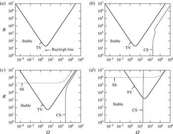
, it is known that a TV mode arises from shear–Coriolis instability (or equivalently centrifugal instability) when the Taylor number exceeds its linear critical value
 ${\it\tau}=106.73$
(Johnston, Halleen & Lezius Reference Johnston, Halleen and Lezius1972). This result is shown in the
 ${\it\Omega}{-}R$
parameter plane by the solid curve in figure 3(a). Along this curve, there exist linear neutral TV mode solutions with wavenumbers
 ${\it\alpha}=0$
and
 ${\it\beta}\approx 1.56$
.
The linear neutral curves in the
 ${\it\Omega}{-}R$
plane for fixed
 $S$
: (a)
 $S=0$
, (b)
 $S=0.4$
, (c)
 $S=4$
and (d)
 $S=40$
. In the regions indicated by ‘Stable’, the basic flow is stable to infinitesimal disturbances with any wavenumber pair
 $({\it\alpha},{\it\beta})$
. The labels TV, CS and SS stand for the Taylor vortex, Coriolis–suction and shear–suction modes, respectively. The neutral disturbance has a longitudinal roll-type structure (
 ${\it\alpha}=0,{\it\beta}\neq 0$
) on the TV mode neutral curve indicated by the solid curve. There are also transverse-roll-type neutral disturbances (
 ${\it\alpha}\neq 0,{\it\beta}=0$
) on the CS and SS modes indicated by the dashed and dotted curves, respectively. The thin dotted line in panel (a) indicates the Rayleigh line
 $R={\it\Omega}$
. The range of truncation level used in the computation is
 $L\in [60,500]$
.

When
 $S$
is increased from zero, different types of instabilities come into existence. To examine the stability against individual modes, we trace the linear neutral curve of each mode by examining the local maximum of
 ${\it\sigma}_{max}$
in the (
 ${\it\alpha},{\it\beta}$
) plane. The overall stability diagrams in the
 ${\it\Omega}{-}R$
plane are shown in figure 3(b–d) for
 $S=0.4$
, 4 and 40, respectively. The parameter region labelled ‘Stable’ corresponds to the linearly stable region for all wavenumbers
 ${\it\alpha}$
and
 ${\it\beta}$
, i.e. the stability region for any infinitesimal disturbance.
Even when
 $S>0$
, the critical wavenumbers of the TV mode are found to keep a longitudinal roll-type structure (i.e. the critical wavenumber
 ${\it\alpha}=0$
). Therefore, in the
 ${\it\Omega}{-}R$
parameter space, the stability criterion can be determined in terms of only the Taylor number
 ${\it\tau}$
; see (2.11). Furthermore, the corresponding stability curves asymptote to the Rayleigh line as
 $R\rightarrow \infty$
(e.g. figure 3
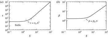
a). As Min & Lueptow (Reference Min and Lueptow1994) and Lahey & Drew (Reference Lahey and Drew2002) pointed out, the effect of suction is to stabilise the basic flow against the TV mode; see solid curves in figure 3. We can also see this trend clearly when the neutral curve is plotted as a function of
 ${\it\tau}$
as in figure 4(a). The figure suggests that there is an asymptotic behaviour of the neutral curve for large
 $S$
. The corresponding critical wavenumber
 ${\it\beta}$
in figure 4(b) and the visualisation of the neutral disturbances in figure 5(a,d) for
 $S=4$
and 40, respectively, reveal that the dominant fluid motion is concentrated at the near-wall region as
 $S$
increases. Note that the horizontal axis is normalised in these figures. In figure 6(a,d), the same flow fields are visualised in a three-dimensional box to emphasise another trend of the TV mode: the flow becomes a short-wavelength structure with increasing
 $S$
. The formal asymptotic theory to be analysed in § 5.1 will demonstrate that the wavenumber is proportional to
 $S$
and the flow is undisturbed outside of the lower wall boundary layer of thickness
 $O(S^{-1})$
.
The TV stability criterion as a function of suction
 $S$
. The solid curves represent the variation of (a) the linear critical Taylor number
 ${\it\tau}$
and (b) the critical wavenumber
 ${\it\beta}$
. The truncation level used in the computation is
 $L=100$
. The asymptotic lines for
 $S\gg 1$
indicated by the thin dotted lines are determined by the optimal values in figure 10(b). The thick grey arrows in panel (a) indicate the bifurcation of the finite-amplitude solutions shown in figure 16(a).

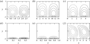
In-plane stream functions of neutral disturbances for (a–c)
 $S=4$
and (d–f)
 $S=40$
: (a,d) TV mode in figure 4; (b,e) SS mode with
 ${\it\Omega}=0$
in figure 7; (c,f) CS mode with
 $R=0$
in figure 8. Note that panel (c) is a
 $\text{CS}_{I}$
mode whilst panel (f) is a
 $\text{CS}_{II}$
mode. The positive (solid) and negative (dashed) isocontours of stream function of in-plane velocity at 20, 40, 60 and 80 % of maximum magnitude are shown. The values of parameters are (a)
 $({\it\tau},{\it\beta})=(720,2.14)$
, (b)
 $(R,{\it\alpha})=(1.94\times 10^{5},0.431)$
, (c)
 $({\it\Omega},{\it\alpha})=(9.18\times 10^{4},1.27)$
, (d)
 $({\it\tau},{\it\beta})=(6.23\times 10^{5},17.5)$
, (e)
 $(R,{\it\alpha})=(1.05\times 10^{6},6.23)$
and (f)
 $({\it\Omega},{\it\alpha})=(358,0.885)$
. Note that the scale of the horizontal axis in each figure is different from that of the wall normal axis.

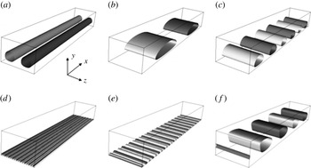
The same plots as in figure 5 but in a box
 $(x,y,z)\in [0,15]\times [-1,1]\times [0,3]$
. The same scale is used in the
 $(x,y,z)$
directions. The light and dark grey surfaces are 60 % maximum and minimum isosurfaces of stream function, respectively.

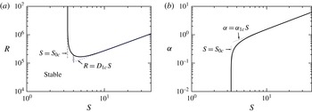
The SS stability criterion as a function of suction
 $S$
. The solid curves are the variation of (a) the linear critical Reynolds number
 $R$
and (b) the critical wavenumber
 ${\it\alpha}$
. Only the case without rotation,
 ${\it\Omega}=0$
, is shown. The truncation level used in the computation is
 $L=140$
. The asymptotic lines indicated by the thin dotted lines are given by the optimal values in figures 10(a) and 13(a). The thick grey arrow in panel (a) indicates the bifurcation of the finite-amplitude solution shown in figure 16(b).

The introduction of a small amount of suction
 $S=0.4$
triggers linear instability with the critical wavenumbers
 ${\it\alpha}\neq 0$
and
 ${\it\beta}=0$
, i.e. transverse-roll-type instability, in the Rayleigh-stable region; see figure 3(b), and further increment of
 $S$
to 4 leads to the appearance of another transverse-roll-type instability in the Rayleigh unstable region as shown in figure 3(c). Hereafter we call the former and latter instabilities Coriolis–suction (CS) and shear–suction (SS) modes, respectively, since CS sets in at
 ${\it\Omega}>R$
and SS at
 ${\it\Omega}<R$
. Our numerical results presented in figure 3(b,c) indicate that the SS and CS mode instabilities are separated from one another by the Rayleigh line for relatively small suction levels. This picture changes when the amount of suction becomes larger. The stability result for
 $S=40$
in figure 3(d) shows that the neutral curve for the CS mode eventually crosses the Rayleigh line whilst that of the SS mode does not.
In order to examine the dependence on
 $S$
of these transverse modes, we draw neutral curves as a function of
 $S$
. The neutral curve of the SS mode is represented at
 ${\it\Omega}=0$
in figure 7(a). Note that in this case Squire’s theorem allows us to consider only disturbances with
 ${\it\beta}=0$
. We confirm that this figure agrees with the linear stability result of plane Couette flow with uniform suction computed by Doering, Spiegel & Worthing (Reference Doering, Spiegel and Worthing2000). The streamwise critical wavenumber seen in figure 7(b) shows two asymptotic behaviours, one at
 $S\gg 1$
and the other at
 $S\approx 3$
. For large values of
 $S$
, the neutral disturbances have short wavelengths as seen in figure 6(b,e). Consistent with the fact that the corresponding formal asymptotic limit to be deduced in § 5.1 coincides with asymptotic suction boundary-layer flow, the visualised disturbances in figure 5(b,e) are confined to the neighbourhood of the suction wall. The other asymptotic behaviour at
 $S\approx 3$
is due to the ‘cut-off’ of instability at finite
 $S$
which corresponds to the long-wavelength limit. The accurate cut-off value of
 $S$
will be examined in § 5.2.
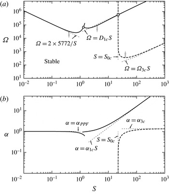
The CS stability criterion as a function of suction
 $S$
. Only the solid-body rotation case,
 $R=0$
, is shown here. The solid and dashed curves are the variation of (a) the linear critical rotation number
 ${\it\Omega}$
and (b) the critical wavenumber
 ${\it\alpha}$
. The solid and dashed curves correspond to the
 $\text{CS}_{I}$
and
 $\text{CS}_{II}$
modes, respectively. The range of truncation level used in the computation is
 $L\in [60,500]$
. The detailed behaviour of the eigenvalue at the points indicated by ‘○’ at
 $(S,{\it\Omega})=(1.3002,6.7030\times 10^{4})$
and ‘▫’ at
 $(S,{\it\Omega})=(22.163,5.7103\times 10^{5})$
is shown in figure 9. The neutral curve starting at
 $S\ll 1$
cannot continue beyond its end point since the corresponding local maximum of growth rate as a function of
 ${\it\alpha}$
, the left hump seen in figure 9(a), vanishes. The other discontinuity at
 $S\approx 1$
is due to the disappearance of the right hump in the same figure. The three asymptotic lines from the right indicated by the thin dotted lines are given by the optimal values in figures 10(a), 11 and 13(b). The leftmost thin dotted asymptotic line is determined by the plane Poiseuille flow result by Orszag (Reference Orszag1971). The thick grey arrows in panel (a) indicate the bifurcation of the finite-amplitude solutions shown in figure 16(c,d).

For the CS mode, the neutral curves are drawn in figure 8 when
 $R=0$
. On the three curves in the figure, the neutral disturbances are found to have the form of transverse rolls (i.e. the critical wavenumber is
 ${\it\beta}=0$
), although it is not possible to apply Squire’s theorem. Therefore, from (2.12), the neutral curve presented in the figure is identical to that of plane Poiseuille flow with uniform suction. As
 $S\rightarrow 0$
, the behaviour of the neutral curve is governed by the Tollmien–Schlichting-wave instability in plane Poiseuille flow without suction; the linear critical values
 $(R_{PPF},{\it\alpha}_{PPF})=(5772,1.02)$
calculated by Orszag (Reference Orszag1971) determine the asymptotic lines shown by
 ${\it\Omega}=2\times 5772S^{-1}$
in figure 8(a) and
 ${\it\alpha}=1.02$
in figure 8(b). Comparing the asymptotic line and neutral curve, we find that the suction stabilises the Tollmien–Schlichting-wave instability as pointed out by Hains (Reference Hains1971) and Sheppard (Reference Sheppard1972). When the effect of suction becomes stronger (
 $S\gtrsim 1$
), two new linear neutral curves appear. As figure 9 shows, where the growth rates at ‘○’ and ‘▫’ in figure 8 are plotted, the neutral curves across ‘○’ arise from the same modes whilst there is a change of instability mechanism at ‘▫’. The instabilities at smaller
 $S$
and larger
 $S$
delimited by ‘▫’ are considered to be modes I and II of plane Poiseuille flow with uniform suction labelled by Fransson & Alfredsson (Reference Fransson and Alfredsson2003b
). Henceforth we call these instabilities
 $\text{CS}_{I}$
and
 $\text{CS}_{II}$
modes. The trend of the critical wavenumbers for
 $S\gg 1$
in figure 8(b) suggests that
 $\text{CS}_{I}$
has a short-wavelength asymptotic behaviour while the critical wavelength of
 $\text{CS}_{II}$
asymptotes to some constant value. The difference can also be found in the appearance of the neutral disturbances shown in figures 5 and 6. As pictured in figure 5(b,c), we find that the neutral disturbance of
 $\text{CS}_{I}$
modes belongs to the same flow regime as the SS mode, which also asymptotes to a short-wavelength structure. In contrast, the visualisation of the neutral disturbance for the
 $\text{CS}_{II}$
mode in figures 5( f) and 6( f) indicates that the fluid vortices occupy the core region. In § 5.2, we shall show that the large-
 $S$
asymptotic limits of these modes are governed by the wall boundary layer and the inviscid core, respectively.
The growth rate
 ${\it\sigma}$
of the critical modes at (a) ‘○’ and (b) ‘▫’ in figure 8(a). The solid and dashed curves correspond to
 $\text{CS}_{I}$
and
 $\text{CS}_{II}$
modes, respectively.

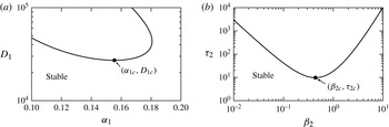
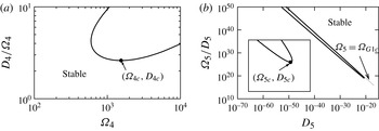
The linear neutral curves of the short-wavelength asymptotic problems for
 $S\gg 1$
. (a) The case (i). The optimal values indicated by the arrow are
 $({\it\alpha}_{1c},D_{1c})=(0.15547,27\,189)$
. (b) The case (ii). The optimal values indicated by the arrow are
 $({\it\beta}_{2c},{\it\tau}_{2c})=(0.43819,9.7352)$
. The truncation level used in the computation is
 $L=60$
.

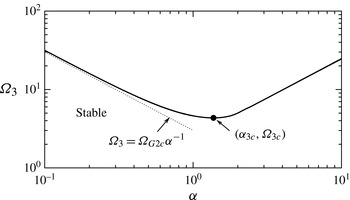
The linear neutral curves of the inviscid problem (5.5). The optimal values indicated by the arrow are
 $({\it\alpha}_{3c},{\it\Omega}_{3c})=(1.3717,4.3457)$
. The truncation level used in the computation is
 $L=60$
. The line indicated by the thin dotted line corresponds to the asymptotic analysis by GDS10.

4. Asymptotic behaviours of the disturbance equations
Motivated by the asymptotic behaviours observed in the last section, here we develop formal asymptotic theories of the governing equations (2.10) assuming at least one of
 $R$
,
 ${\it\Omega}$
and
 $S$
are asymptotically large. The nonlinear asymptotic theories in the following are relatively simple since no internal layer singularity such as a critical layer is involved. When
 $S$
is asymptotically large, the fluid layer is divided into the boundary layer of thickness
 $O(S^{-1})$
and the core layer of thickness
 $O(1)$
due to the behaviour of the basic flow (2.6). For each of the layers, a reduced problem can be derived from the Navier–Stokes equations. The overall flow dynamics is determined by one of the layers and the other layer plays only a passive role dynamically.
4.1. The long-wavelength limit
We first seek a single set of equations that is valid for the entire fluid layer assuming
 $S\sim O(1)$
. Considering the balance of the nonlinear and dissipation terms, the flow must have a long wavelength. The wavenumber
 $k=\sqrt{{\it\alpha}^{2}+{\it\beta}^{2}}$
is assumed to be asymptotically small (
 $k\ll 1$
) and at least one of
 $R$
and
 ${\it\Omega}$
are of
 $O(k^{-1})$
in this subsection. Defining the scaled variables as
 $[u,v,w,p,x,y,z,t]\rightarrow [ku,v,kw,k^{2}p,kx,y,kz,t]$
(hereafter this notation means switching the variables as
 $[{\hat{u}},\dots ]=[ku,\dots ]$
in the governing equations and then all of the circumflexes are dropped from the equations for convenience) and collecting the leading-order terms, we find
 $$\begin{eqnarray}\left.\begin{array}{@{}c@{}}\{\partial _{t}+(u_{b0}+u)\partial _{x}+(v-S)\partial _{y}+w\partial _{z}\}u+(u_{b0}^{\prime }-{\it\Omega}_{0})v=-\partial _{x}p+\partial _{yy}^{2}u,\\ {\it\Omega}_{0}u=-\partial _{y}p,\\ \{\partial _{t}+(u_{b0}+u)\partial _{x}+(v-S)\partial _{y}+w\partial _{z}\}w=-\partial _{z}p+\partial _{yy}^{2}w,\\ \partial _{x}u+\partial _{y}v+\partial _{z}w=0,\end{array}\right\}\end{eqnarray}$$
where
 $$\begin{eqnarray}u_{b0}(y)={\it\Omega}_{0}(1+y)+2(R_{0}-{\it\Omega}_{0})\frac{1-\text{e}^{-S(1+y)}}{1-\text{e}^{-2S}}\end{eqnarray}$$
is the scaled basic flow depending on parameters
 $R_{0}\equiv kR$
and
 ${\it\Omega}_{0}\equiv k{\it\Omega}$
. The boundary conditions are
 $$\begin{eqnarray}u=v=w=0\quad \text{at}\ y=\pm 1.\end{eqnarray}$$
The reduced problem has four parameters:
 ${\it\theta}_{0}\equiv \arctan ({\it\beta}/{\it\alpha})$
,
 $R_{0}$
,
 ${\it\Omega}_{0}$
and
 $S$
.
The system (4.1), valid for
 ${\it\alpha}\sim O(R^{-1})$
and
 ${\it\beta}\sim O(R^{-1})$
, and the asymptotically reduced system recently studied by Deguchi, Hall & Walton (Reference Deguchi, Hall and Walton2013), where
 ${\it\alpha}\sim O(R^{-1})$
and
 ${\it\beta}\sim O(1)$
are considered, are natural nonlinear three-dimensional extensions of the linear long-wavelength stability problem in Cowley & Smith (Reference Cowley and Smith1985). These nonlinear systems are essentially the parabolic asymptotic equations considered in boundary-layer flow, see Luchini (Reference Luchini1996) for example. The crucial difference between the two nonlinear systems is that, when
 $R$
is asymptotically large, the former equation (4.1) allows
 ${\it\Omega}$
of
 $O(R)$
whilst the latter reduced system by Deguchi et al. (Reference Deguchi, Hall and Walton2013) breaks down when
 ${\it\Omega}$
is larger than
 $O(R^{-1})$
.
4.2. The short-wavelength limits
As we noted in § 2, the basic flow has distinct wall and core layer structures for asymptotically large
 $S\ (S\gg 1)$
. The behaviours of the basic flow in the wall and core layers are governed by
 $D=R-{\it\Omega}$
and
 ${\it\Omega}$
, respectively; see (2.8) and (2.9). When we assume that the fluid motion is dominant in the wall layer, as seen in TV, SS and
 $\text{CS}_{I}$
results in § 3, it is natural to regard the order of streamwise and spanwise wavelengths as comparable to the
 $O(S^{-1})$
boundary-layer thickness. Depending on the assumptions for the asymptotic properties of
 $D$
and
 ${\it\Omega}$
, we can consider two cases as follows.
Case (i)
 ${\it\Omega}\sim O(S)$
and
$D\sim O(S)$


The scaling
 $[u,v,w,p,x,y,z,t]\rightarrow [S^{-1}u,S^{-1}v,S^{-1}w,S^{-2}p,Sx-2DSt,y,Sz,S^{2}t]$
reduces the governing equations (2.10) to
 $$\begin{eqnarray}\left.\begin{array}{@{}c@{}}\{\partial _{t}+({\it\Omega}_{1}(1+y)+u)\partial _{x}+w\partial _{z}\}u=-\partial _{x}p+(\partial _{xx}^{2}+\partial _{zz}^{2})u,\\ \{\partial _{t}+({\it\Omega}_{1}(1+y)+u)\partial _{x}+w\partial _{z}\}v=(\partial _{xx}^{2}+\partial _{zz}^{2})v,\\ \{\partial _{t}+({\it\Omega}_{1}(1+y)+u)\partial _{x}+w\partial _{z}\}w=-\partial _{z}p+(\partial _{xx}^{2}+\partial _{zz}^{2})w,\\ \partial _{x}u+\partial _{z}w=0,\end{array}\right\}\end{eqnarray}$$
to leading order, where
 $(1-y)\sim O(1)$
is assumed and
 ${\it\Omega}_{1}\equiv S^{-1}{\it\Omega}$
is the scaled system rotation rate. We can construct the Reynolds–Orr energy equation of (4.4) given by
 $$\begin{eqnarray}{\textstyle \frac{1}{2}}\partial _{t}\langle u^{2}+v^{2}+w^{2}\rangle =-\langle (\partial _{x}u)^{2}+(\partial _{z}u)^{2}+(\partial _{x}v)^{2}+(\partial _{z}v)^{2}+(\partial _{x}w)^{2}+(\partial _{z}w)^{2}\rangle <0,\end{eqnarray}$$
where
 $\langle \ast \rangle$
is the volumetric average operator in a periodic box. The new streamwise coordinate
 $x$
moves with ‘free-stream speed’
 $2D$
in the boundary-layer part of the basic flow (see (2.9)) so that the equations take the simplest form. Since (4.5) does not have an energy input, the size of the disturbance must monotonically decay in the core layer.
Non-trivial dynamics appears only in the thin boundary layer adjacent to the lower suction wall after a sufficiently long time has passed. In this wall layer, where the variables
 $[U,V,W,P,X,Y,Z,T]\rightarrow [\!S^{-1}u,S^{-1}v,S^{-1}w,S^{-2}p,Sx-2DSt,$
 $S(1+y),Sz,S^{2}t\!]$
are of
 $O(1)$
, the leading-order equations become
 $$\begin{eqnarray}\left.\begin{array}{@{}c@{}}\{\partial _{T}+(U-2D_{1}\text{e}^{-Y})\partial _{X}+(V-1)\partial _{Y}+W\partial _{Z}\}U-2D_{1}\text{e}^{-Y}V=-\partial _{X}P+{\rm\Delta}U,\\ \{\partial _{T}+(U-2D_{1}\text{e}^{-Y})\partial _{X}+(V-1)\partial _{Y}+W\partial _{Z}\}V=-\partial _{Y}P+{\rm\Delta}V,\\ \{\partial _{T}+(U-2D_{1}\text{e}^{-Y})\partial _{X}+(V-1)\partial _{Y}+W\partial _{Z}\}W=-\partial _{Z}P+{\rm\Delta}W,\\ \partial _{X}U+\partial _{Y}V+\partial _{Z}W=0,\end{array}\right\}\end{eqnarray}$$
where
 $D_{1}\equiv S^{-1}(R-{\it\Omega})$
and
 ${\rm\Delta}$
is now defined as
 $\partial _{XX}^{2}+\partial _{YY}^{2}+\partial _{ZZ}^{2}$
. To satisfy the no-slip conditions and the matching conditions to the core solution,
 $u=v=w\equiv 0$
, we require the boundary conditions
 $$\begin{eqnarray}U=V=W=0\quad \text{at}\ Y=0,\infty .\end{eqnarray}$$
Note that the system (4.6), which has parameters
 $D_{1}$
,
 ${\it\alpha}_{1}\equiv S^{-1}{\it\alpha}$
and
 ${\it\beta}_{1}\equiv S^{-1}{\it\beta}$
, coincides with the governing equations of the unbounded asymptotic suction boundary-layer flow problem with the Reynolds number
 $D_{1}$
.
Case (ii)
${\it\Omega}\sim O(S^{2})$
and
$D\sim O(S)$


When the system rotation rate
 ${\it\Omega}$
is stronger than in case (i), another valid asymptotic equation can be made. The scaling
 $[u,v,w,p,x,y,z,t]\rightarrow [\!S^{-2}u,S^{-2}v,$
 $S^{-1}w,S^{-3}p,x,y,Sz,S^{2}t\!]$
to (2.10) yields the leading-order equations in the core layer,
 $$\begin{eqnarray}\left.\begin{array}{@{}c@{}}\{\partial _{t}+({\it\Omega}_{2}(1+y)+u)\partial _{x}+v\partial _{y}+w\partial _{z}\}u=\partial _{zz}^{2}u,\\ \{\partial _{t}+({\it\Omega}_{2}(1+y)+u)\partial _{x}+v\partial _{y}+w\partial _{z}\}v+{\it\Omega}_{2}u=\partial _{zz}^{2}v,\\ 0=-\partial _{z}\,p,\\ \partial _{x}u+\partial _{y}v+\partial _{z}w=0,\end{array}\right\}\end{eqnarray}$$
where
 ${\it\Omega}_{2}\equiv S^{-2}{\it\Omega}$
. The energy balance of the
 $x$
-momentum equation of (4.8),
 $$\begin{eqnarray}{\textstyle \frac{1}{2}}\partial _{t}\langle u^{2}\rangle =-\langle (\partial _{z}u)^{2}\rangle <0,\end{eqnarray}$$
allows us to set
 $u=0$
. In this case, the
 $y$
-momentum balance of (4.8) yields
 $$\begin{eqnarray}{\textstyle \frac{1}{2}}\partial _{t}\langle v^{2}\rangle =-\langle (\partial _{z}v)^{2}\rangle <0,\end{eqnarray}$$
and together with the continuity constraint,
 $\partial _{z}w$
tends to zero when
 $u$
and
 $v$
vanish. The only velocity component that survives at this stage is the
 $z$
-averaged part of
 $w$
,
 $\breve{w}(x,y)=({\it\beta}/2{\rm\pi})\int _{0}^{2{\rm\pi}/{\it\beta}}w\text{d}z$
. The velocity component
 $\breve{w}(x,y)$
also decays, since, when
 $\boldsymbol{u}$
tends to
 $\breve{w}\boldsymbol{e}_{z}$
, the next-order
 $z$
-momentum equation of (2.10) yields
 $$\begin{eqnarray}{\textstyle \frac{1}{2}}\partial _{t}\langle \breve{w}^{2}\rangle =-\langle (\partial _{x}\breve{w})^{2}+(\partial _{y}\breve{w})^{2}\rangle <0.\end{eqnarray}$$
Therefore, after some transient motion, the disturbance
 $\boldsymbol{u}$
must vanish outside the boundary layer.
Transforming into wall layer variables as
 $[U,V,W,P,X,Y,Z,T]\rightarrow [\!{\it\Omega}_{2}S^{-1}u,S^{-1}v,$
 $S^{-1}w,S^{-2}p,x,S(1+y),Sz,S^{2}t\!]$
, the leading-order equations become
 $$\begin{eqnarray}\left.\begin{array}{@{}c@{}}\{\partial _{T}+(V-1)\partial _{Y}+W\partial _{Z}\}U+2{\it\tau}_{2}\text{e}^{-Y}V=(\partial _{YY}^{2}+\partial _{ZZ}^{2})U,\\ \{\partial _{T}+(V-1)\partial _{Y}+W\partial _{Z}\}V+U=-\partial _{Y}P+(\partial _{YY}^{2}+\partial _{ZZ}^{2})V,\\ \{\partial _{T}+(V-1)\partial _{Y}+W\partial _{Z}\}W=-\partial _{Z}P+(\partial _{YY}^{2}+\partial _{ZZ}^{2})W,\\ \partial _{Y}V+\partial _{Z}W=0,\end{array}\right\}\end{eqnarray}$$
where
 ${\it\tau}_{2}\equiv S^{-3}{\it\tau}=S^{-3}{\it\Omega}(R-{\it\Omega})$
. The boundary conditions are the same as (4.7). This system, which is independent of streamwise variable
 $X$
and has two parameters
 ${\it\tau}_{2}$
and
 ${\it\beta}_{2}\equiv S^{-1}{\it\beta}$
, takes a form similar to the Görtler vortex equations derived by Hall (Reference Hall1988), although here the vortex is driven by the Coriolis force instead of wall curvature. In the presence of uniform suction, Hall’s formulation becomes that studied by Park & Huerre (Reference Park and Huerre1995), where the system coincides with (4.12) except for the driving mechanism.
4.3. The inviscid limit
Here we consider a situation where the overall fluid dynamics is determined by the core layer when
 $S\gg 1$
, as we observed for the
 $\text{CS}_{II}$
mode. In this case, it is reasonable to set the wavelengths
 ${\sim}O(1)$
with
 ${\it\Omega}\sim O(S)$
and
 $D\sim O(S)$
. The scaling we adopt here is
 $[u,v,w,p,x,y,z,t]\rightarrow [S^{-1}u,S^{-1}v,S^{-1}w,S^{-2}p,x-2Dt,y,z,St]$
. The equations are inviscid up to the leading order:
 $$\begin{eqnarray}\left.\begin{array}{@{}c@{}}\{\partial _{t}+({\it\Omega}_{3}(1+y)+u)\partial _{x}+(v-1)\partial _{y}+w\partial _{z}\}u=-\partial _{x}p,\\ \{\partial _{t}+({\it\Omega}_{3}(1+y)+u)\partial _{x}+(v-1)\partial _{y}+w\partial _{z}\}v+{\it\Omega}_{3}u=-\partial _{y}p,\\ \{\partial _{t}+({\it\Omega}_{3}(1+y)+u)\partial _{x}+(v-1)\partial _{y}+w\partial _{z}\}w=-\partial _{z}p,\\ \partial _{x}u+\partial _{y}v+\partial _{z}w=0,\end{array}\right\}\end{eqnarray}$$
where
 ${\it\Omega}_{3}\equiv S^{-1}{\it\Omega}$
. The new streamwise coordinate
 $x$
moves with speed of
 $2D$
as in the last subsection. The boundary conditions at the upper blowing wall are given by the no-slip conditions whilst those on approaching the lower suction wall are to be given by the matching conditions to the wall layer solution.
The scaling is changed as
 $[U,V,W,P,X,Y,Z,T]\rightarrow [\!S^{-1}u,v,S^{-1}w,S^{-3}p,x-2Dt,$
 $S(1+y),z,St\!]$
to yield the leading-order equations in the lower boundary layer,
 $$\begin{eqnarray}\left.\begin{array}{@{}c@{}}-\partial _{Y}U=-\partial _{X}P+\partial _{YY}^{2}U,\\ -\partial _{Y}W=-\partial _{Z}P+\partial _{YY}^{2}W,\\ 0=-\partial _{Y}P,\\ \partial _{X}U+\partial _{Y}V+\partial _{Z}W=0,\end{array}\right\}\end{eqnarray}$$
and the boundary conditions
 $$\begin{eqnarray}U=V=W=0\quad \text{at}\ Y=0\end{eqnarray}$$
on the lower wall. The solution to these equations can be written as
 $[U,V,W]=[\widetilde{U}(1-\text{e}^{-Y}),\widetilde{V}(Y-1+\text{e}^{-Y}),\widetilde{W}(1-\text{e}^{-Y})]$
where
 $[\widetilde{U},\widetilde{V},\widetilde{W}](X,Z)$
are
 $O(1)$
functions that satisfy
 $\partial _{X}\widetilde{U}+\widetilde{V}+\partial _{Z}\widetilde{W}=0$
. The leading-order matching conditions require the core solutions
 $[u,v,w]$
to behave like
 $[\widetilde{U},\widetilde{V}(1+y),\widetilde{W}]$
as
 $y\rightarrow -1$
, i.e. the core solutions only satisfy
 $v=0$
on approaching the lower wall, and passive fluid movement in the thin wall layer adjusts the whole flow to the no-slip conditions.
Note that the inviscid equations (4.13) have parameters
 ${\it\Omega}_{3}$
,
 ${\it\alpha}$
and
 ${\it\beta}$
and are different from the Euler equations. We shall show that the linear stability of (4.13) does not coincide with the Rayleigh stability criterion in the next section.
5. Linear stability analysis of the asymptotic problems
The asymptotic problems in the last section can be numerically solved by a spectral method similar to that used for the full Navier–Stokes case. The following subsections investigate the linear stability of the reduced problems. The results show excellent agreement with the asymptotic behaviours of the linear neutral curves in § 3, confirming the validity of the reduction process in § 4.
5.1. The asymptotic behaviours of the linear instability for large suction
First we solve the short-wavelength problems (4.6) and (4.12), together with the corresponding boundary conditions in order to find the large-
 $S$
asymptotic behaviour seen in the full Navier–Stokes neutral curves of TV, SS and
 $\text{CS}_{I}$
modes. Recall that the asymptotic theories for these modes in § 4.2 showed that there is no core disturbance at the asymptotic limit; see also figures 5 and 6 for evidence from the full Navier–Stokes computation. The corresponding short-wavelength linearised potential equations in the wall boundary layer comprise
 $$\begin{eqnarray}\left(\left(s-2\text{i}{\it\alpha}_{1}D_{1}\text{e}^{-Y}-\frac{\text{d}}{\text{d}Y}\right)\left(\frac{\text{d}^{2}}{\text{d}Y^{2}}-{{\it\alpha}_{1}}^{2}\right)-2\text{i}{\it\alpha}_{1}D_{1}\text{e}^{-Y}-\left(\frac{\text{d}^{2}}{\text{d}Y^{2}}-{{\it\alpha}_{1}}^{2}\right)^{2}\right){\it\Phi}=0\end{eqnarray}$$
and
 $$\begin{eqnarray}\left.\begin{array}{@{}l@{}}\left(s-\displaystyle \frac{\text{d}}{\text{d}Y}-\left(\displaystyle \frac{\text{d}^{2}}{\text{d}Y^{2}}-{{\it\beta}_{2}}^{2}\right)\right)\left(\displaystyle \frac{\text{d}^{2}}{\text{d}Y^{2}}-{{\it\beta}_{2}}^{2}\right){\it\Phi}+\text{i}{\it\beta}_{2}{\it\Psi}=0,\\ \left(s-\displaystyle \frac{\text{d}}{\text{d}Y}-\left(\frac{\text{d}^{2}}{\text{d}Y^{2}}-{{\it\beta}_{2}}^{2}\right)\right){\it\Psi}-2\text{i}{\it\beta}_{2}{\it\tau}_{2}\text{e}^{-Y}{\it\Phi}=0,\end{array}\right\}\end{eqnarray}$$
respectively, where subscripts 1 and 2 correspond to cases (i) and (ii) in § 4.2 and we assume
 ${\it\beta}_{1}=0$
in case (i), invoking the results for the SS and
 $\text{CS}_{I}$
modes in § 3. Note that the reduced problem for case (ii) is streamwise independent as TV mode. The boundary conditions for the eigenfunctions
 ${\it\Phi}$
and
 ${\it\Psi}$
are chosen as
 $$\begin{eqnarray}{\it\Phi}={\it\Phi}^{\prime }={\it\Psi}=0\quad \text{at}\ Y=0,\infty ,\end{eqnarray}$$
so that condition (4.7) is satisfied. The problems in the semi-infinite domain can be solved by using the map
 $$\begin{eqnarray}Y=q\frac{1+{\it\eta}}{1-{\it\eta}},\end{eqnarray}$$
which transforms
 $Y\in [0,\infty ]$
to
 ${\it\eta}\in [-1,1]$
(Boyd Reference Boyd2001), where the mapping parameter
 $q$
is chosen to be unity throughout the paper. For the short-wavelength limit problems, (5.1) and (5.2), the basis functions (3.6) and the collocation points (3.7) are used for the expansion in the
 ${\it\eta}$
coordinate. The collocation method results in the neutral curves for the case (i) and (ii) short-wavelength limit problems presented in figure 10(a,b), respectively. By using the optimum values
 $({\it\alpha}_{1c},D_{1c})$
and
 $({\it\beta}_{2c},{\it\tau}_{2c})$
in the figures, the asymptotic lines for SS,
 $\text{CS}_{I}$
and TV modes are drawn as the thin dotted lines in figures 4, 7 and 8. The former critical value
 $({\it\alpha}_{1c},D_{1c})$
is consistent with the linear stability of asymptotic suction boundary-layer flow obtained by Hocking (Reference Hocking1975), Drazin & Reid (Reference Drazin and Reid1981) and Fransson & Alfredsson (Reference Fransson and Alfredsson2003a
).
The linear stability of inviscid limit equations (4.13) for
 $S\gg 1$
can also be obtained by solving
 $$\begin{eqnarray}\left(s+\text{i}{\it\alpha}{\it\Omega}_{3}(1+y)-\frac{\text{d}}{\text{d}y}\right)\left(\frac{\text{d}^{2}}{\text{d}y^{2}}-{\it\alpha}^{2}\right){\it\Phi}=0,\end{eqnarray}$$
subject to the boundary conditions
 $$\begin{eqnarray}\left.\begin{array}{@{}ll@{}}{\it\Phi}={\it\Phi}^{\prime }=0 & \quad \text{at}\ y=1,\\ {\it\Phi}=0 & \quad \text{at}\ y=-1.\end{array}\right\}\end{eqnarray}$$
As described in § 4.3, the no-slip conditions at the lower wall are taken care of by the boundary-layer solution. Discretising (5.5) at collocation points (3.7) with appropriate basis functions
 $$\begin{eqnarray}{\it\Phi}_{l}(y)=(1-y^{2})(1-y)T_{l}(y),\quad {\it\Psi}_{l}(y)=(1-y)T_{l}(y),\end{eqnarray}$$
the stability curve is drawn in figure 11. The optimal values
 $({\it\alpha}_{3c},{\it\Omega}_{3c})$
give the large-
 $S$
asymptotic line of the
 $\text{CS}_{II}$
linear stability boundary indicated by the thin dotted line in figure 8.
The scaling
 ${\it\Omega}\sim O(S),\ R\sim O(S)$
used for both the case (i) short-wavelength limit and the inviscid limit allows us to plot the large-
 $S$
linear stability boundaries of SS and CS modes in the scaled
 ${\it\Omega}{-}R$
plane as in figure 12. Note that TV mode instability, which has the scaling
 ${\it\Omega}\sim O(S^{2})$
, does not appear in this figure. Therefore, for asymptotically large
 $S$
, the linearly stable region is bounded by the SS and
 $\text{CS}_{II}$
modes.
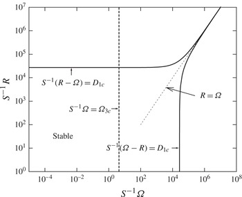
The large-
 $S$
asymptotic behaviour of the neutral curves in the scaled
 ${\it\Omega}{-}R$
plane. The two solid lines, which correspond to the SS and
 $\text{CS}_{I}$
modes, are drawn by using the case (i) short-wavelength asymptotic result (the optimised value in figure 10
a). The dashed line is the inviscid asymptotic result of the
 $\text{CS}_{II}$
mode (the optimised value in figure 11). The Rayleigh line
 $R={\it\Omega}$
is traced as the thin dotted line.

Now from figure 12 we can explain the origin of the distinct behaviours of
 $\text{CS}_{I}$
and
 $\text{CS}_{II}$
modes observed in figure 3. The neutral curves of SS and
 $\text{CS}_{I}$
modes drawn by the solid lines cannot cross the Rayleigh line
 $R={\it\Omega}$
, since both of them obey the case (i) short-wavelength scaling. In contrast, the inviscid limit asymptotic result clearly proves that the neutral curve of
 $\text{CS}_{II}$
mode drawn by the dashed line does not have such a restriction.
5.2. The long-wavelength cut-offs of the linear instabilities
By solving the reduced problem (4.1) in the long-wavelength limit, we can calculate the accurate cut-off suction values of the linear neutral curves for the SS and
 $\text{CS}_{II}$
modes. Assuming that the flow is independent of
 $z$
, i.e.
 ${\it\theta}_{0}=0$
, the Orr–Sommerfeld equation of the reduced system (4.1) can be written as
 $$\begin{eqnarray}\left(\left(s+\text{i}u_{b0}-S\frac{\text{d}}{\text{d}y}\right)\frac{\text{d}^{2}}{\text{d}y^{2}}-\text{i}u_{b0}^{\prime \prime }-\frac{\text{d}^{4}}{\text{d}y^{4}}\right){\it\Phi}=0.\end{eqnarray}$$
The boundary conditions are
 $$\begin{eqnarray}{\it\Phi}={\it\Phi}^{\prime }=0\quad \text{at}\ y=\pm 1.\end{eqnarray}$$
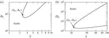
We can solve (5.8) numerically by using basis functions (3.6) and collocation points (3.7). The cut-off value of
 $S$
for the SS mode in figure 7, indicated as
 $S=S_{0c}$
, can be obtained by minimising
 $S$
along the stability curve of the long-wavelength problem (5.8) with
 ${\it\Omega}_{0}=0$
for
 $u_{b0}(y)$
in (4.2), as presented in figure 13(a). Similarly, the cut-off value of the
 $\text{CS}_{II}$
mode in figure 8 can be obtained by solving (5.8) with
 $R_{0}=0$
for
 $u_{b0}(y)$
as shown in figure 13(b).
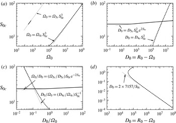
The linear neutral curves of the long-wavelength limit problem (5.8). (a) The SS mode for
 ${\it\Omega}_{0}=0$
, which gives the parameter value at cut-off
 $(S_{0c},R_{0c})=(3.3511,90\,015)$
. (b) The CS mode for
 $R=0$
, where the parameter values at cut-off are
 $(S_{0c},{\it\Omega}_{0c})=(22.163,255.36)$
. The truncation level used in the computation is
 $L=140$
.

When these analyses are generalised for non-zero
 $R_{0}$
and
 ${\it\Omega}_{0}$
, the cut-off suction value
 $S_{0c}$
becomes a function of the ratio
 $R_{0}/{\it\Omega}_{0}$
and can also be determined as a result of minimisation of
 $S$
along the neutral curve in the
 $S{-}R_{0}$
or
 $S{-}{\it\Omega}_{0}$
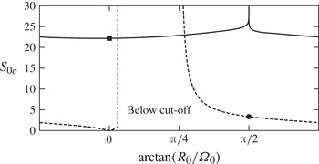
planes. The variation of the cut-off value
 $S_{0c}$
as a function of
 $\arctan (R_{0}/{\it\Omega}_{0})$
is shown in figure 14. Note that the solid and dashed curves in the figure, continued from the cut-off values of the
 $\text{CS}_{II}$
and SS modes in figure 13 respectively, must have period
 ${\rm\pi}$
. The parameter region for
 $\arctan (R_{0}/{\it\Omega}_{0})\in [0,{\rm\pi}/2]$
corresponds to the anticyclonic case. The figure shows that the appearance of the
 $\text{CS}_{II}$
mode is quite abrupt with increasing suction: this mode appears at
 $S=S_{0c}\approx 22.1$
near the solid-body rotation case and exists across the Rayleigh line at
 $S=S_{0c}\approx 22.9$
; see also figures 3 and 8. Another interesting feature of figure 14 is blow-up behaviours of the cut-off thresholds at
 $\arctan (R_{0}/{\it\Omega}_{0})\approx 0.03{\rm\pi}$
,
 ${\rm\pi}/4$
and
 ${\rm\pi}/2$
. The blow-up points at
 $\arctan (R_{0}/{\it\Omega}_{0})\approx {\rm\pi}/4$
and
 ${\rm\pi}/2$
correspond to dual limits of long-wavelength and large suction, which are not described in § 4. The detailed analyses of the dual limit problems are given in appendix A.
The variation of the long-wavelength cut-off suction value
 $S_{0c}$
of the linear instability as a function of
 $\arctan (R_{0}/{\it\Omega}_{0})$
. The solid and dashed lines correspond to the
 $\text{CS}_{II}$
and SS modes, respectively. Note that
 $\arctan (R_{0}/{\it\Omega}_{0})=0,{\rm\pi}/4$
and
 ${\rm\pi}/2$
correspond to
 $R_{0}=0,\ R_{0}={\it\Omega}_{0}$
and
 ${\it\Omega}_{0}=0$
, respectively. Symbols: ▪,
 $\text{CS}_{II}$
, and ●, SS in figure 13. The range of truncation level used in the computation is
 $L\in [100,500]$
.

5.3. Comparison with the asymptotic results of GDS10
Two types of asymptotic analyses of Taylor–Couette flow with large radial suction have been carried out by GDS10, assuming infinitesimally narrow gap for a fixed azimuthal wavenumber. Since the azimuthal wavenumber they used is based on an angle whilst our wavenumber
 ${\it\alpha}$
is based on length normalised by the half gap distance, their asymptotic limits correspond to the special case of large-
 $S$
and long-wavelength limits of our model. In fact, one of the asymptotic equations in GDS10 can be obtained by taking the limit of
 $D_{5}\rightarrow 0$
in the dual limit equation (A 5) in appendix A, leading to
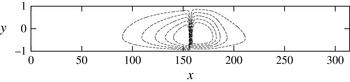
 $$\begin{eqnarray}\left(s-\text{i}{\it\Omega}_{G1}Y+\frac{\text{d}}{\text{d}Y}-\frac{\text{d}^{2}}{\text{d}Y^{2}}\right)\frac{\text{d}^{2}{\it\Phi}}{\text{d}Y^{2}}=0,\end{eqnarray}$$
where
 ${\it\Omega}_{G1}\equiv {\it\Omega}_{5}$
. In addition to the upper wall layer where
 $Y=S(1-y)\sim O(1)$
and (5.10) is valid, there are a core layer, where
 ${\it\Phi}$
has a linear profile, and a lower wall layer of thickness
 $O(S^{-3/2})$
as in the last subsection. The other asymptotic equation in GDS10,
 $$\begin{eqnarray}\left(s+\text{i}{\it\Omega}_{G2}(1+y)-\frac{\text{d}}{\text{d}y}\right)\frac{\text{d}^{2}{\it\Phi}}{\text{d}y^{2}}=0,\end{eqnarray}$$
can be found by keeping
 ${\it\Omega}_{G2}\equiv {\it\alpha}{\it\Omega}_{3}$
as
 $O(1)$
and taking
 ${\it\alpha}\rightarrow 0$
in our inviscid limit equation (5.5). The results by GDS10, evaluated as
 ${\it\Omega}_{G1c}=0.0953$
and
 ${\it\Omega}_{G2c}=3.01$
in our context, describe the asymptotic behaviours of the long-wavelength
 $\text{CS}_{II}$
mode instability.
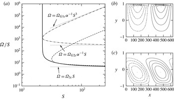
In order to compare our result with figure 7(a) of GDS10, the linear neutral curve of the
 $\text{CS}_{II}$
mode in our figure 8 is replotted as a function of
 $S$
and
 ${\it\Omega}/S$
as the solid curves in figure 15(a). By definition, the neutral curves for fixed
 ${\it\alpha}$
, drawn by dashed and dot-dashed curves for
 ${\it\alpha}=0.885$
and 0.01, respectively, are nested in this solid curve. When
 ${\it\Omega}/S$
is increased, the disturbance with the wavenumber
 ${\it\alpha}$
destabilises the basic flow and then stabilises it. The asymptotic lines defined by
 ${\it\Omega}_{G1c}$
and
 ${\it\Omega}_{G2c}$
represent the destabilising and stabilising boundaries, respectively. The smaller
 ${\it\alpha}$
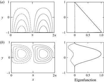
, the better approximation the asymptotic lines have. It has been reported in GDS10 that the solution of (5.10) has a vortex structure near the blowing wall whilst in the solution of (5.11) vortices emerge at the fluid core. In the corresponding full Navier–Stokes results in figure 15(b,c), where the neutral eigenmodes are shown for
 $S=100$
and
 ${\it\alpha}=0.01$
, we can see the asymptotic structures described in GDS10. The analysis here conclusively shows that the instability found by GDS10 is a special case of the
 $\text{CS}_{II}$
mode.
(a) Comparison of the neutral curves of the
 $\text{CS}_{II}$
mode for
 ${\it\alpha}=0.885$
(dashed line),
 ${\it\alpha}=0.01$
(dot-dashed line) and all
 ${\it\alpha}$
(solid line). The uppermost two thin dotted lines correspond to the asymptotic results by GDS10 with
 ${\it\alpha}=0.01$
. The lowest thin dotted line is determined by
 ${\it\Omega}_{3c}$
given in figure 11. (b,c) The stream functions of the neutral modes for
 $({\it\alpha},S)=(0.01,100)$
, corresponding to (b) the upper neutral point at
 ${\it\Omega}\approx 8.44\times 10^{6}$
and (c) the lower neutral point at
 ${\it\Omega}\approx 3.83\times 10^{4}$
. The definitions of the solid and dotted lines are the same as in figure 5.

6. The nonlinear analysis
Our concern in this section is transition from the basic state triggered by finite-amplitude disturbances. This type of transition typically occurs when finite-amplitude solutions bifurcate subcritically and continue to exist in the linearly stable regime. One of the possible ways to find finite-amplitude solutions is by means of bifurcation analysis at a linear critical point. Bifurcating solutions must inherit the property of the corresponding neutral eigenmode. For example, the neutral curves of the TV mode in § 3 were always determined by
 ${\it\alpha}=0$
with purely real eigenvalues. In this case, bifurcation of a steady longitudinal roll-type solution, which can be approximated by the Fourier–Chebyshev expansions
 $$\begin{eqnarray}\left.\begin{array}{@{}c@{}}\displaystyle {\it\phi}(x,y,z,t)=\mathop{\sum }\limits_{l=0}^{L}\mathop{\sum }\limits_{n=1}^{N}X_{ln}^{(1)}\exp (\text{i}n{\it\beta}z){\it\Phi}_{l}(y)+\text{c.c.},\\ \displaystyle {\it\psi}(x,y,z,t)=\mathop{\sum }\limits_{l=0}^{L}\mathop{\sum }\limits_{n=1}^{N}X_{ln}^{(2)}\exp (\text{i}n{\it\beta}z){\it\Psi}_{l}(y)+\text{c.c.},\\ \displaystyle \overline{u}(y)=\mathop{\sum }\limits_{l=0}^{L}X_{l0}^{(1)}{\it\Psi}_{l}(y),\\ \overline{w}(y)=0,\end{array}\right\}\end{eqnarray}$$
is expected. Here c.c. stands for complex conjugate and
 $(L,N)$
is the truncation level, where systematic resolution tests have been performed to determine the value of
 $(L,N)$
such that the results in this section are adequately resolved. The basis functions
 ${\it\Phi}_{l}(y)$
and
 ${\it\Psi}_{l}(y)$
are chosen to be those used in the linear analysis, (3.6). Substitution of expressions (6.1) into (2.15)–(2.18) results in a set of nonlinear algebraic equations for coefficients
 $X_{ln}^{(j)}$
, which can be solved by a Newton–Raphson iterative method. In order to measure how much the solutions differ from the unperturbed basic flow, we introduce the norm of mean-flow distortion,
 $$\begin{eqnarray}{\it\Delta}=\sqrt{\frac{1}{2}\int _{-1}^{1}\overline{u}^{2}\text{d}y}.\end{eqnarray}$$
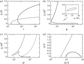
The bifurcation of the TV mode solution at the neutral curve in figure 4 is drawn in figure 16(a), where
 ${\it\Delta}$
is scaled by
 ${\it\Omega}$
so that the result depends only on the parameters
 ${\it\tau}$
,
 $S$
and
 ${\it\beta}$
. Here and hereafter, wavenumbers equal to the linear critical value are chosen unless otherwise noted. We find that the bifurcation type changes from supercritical to subcritical if
 $S$
is greater than
 ${\approx}1.69$
; see figure 16(a), where the numerical results for
 $S=1.69$
and
 $S=4$
are depicted by the dashed and solid lines, respectively. Despite the slight subcriticality, the branch of the TV mode cannot cross the Rayleigh line where
 ${\it\tau}=0$
.
We can also investigate bifurcations of the SS and CS finite-amplitude solutions assuming the following expansions:
 $$\begin{eqnarray}\left.\begin{array}{@{}c@{}}\displaystyle {\it\phi}(x,y,z,t)=\mathop{\sum }\limits_{l=0}^{L}\mathop{\sum }\limits_{n=1}^{N}X_{ln}^{(1)}\exp (\text{i}n{\it\alpha}(x-ct)){\it\Phi}_{l}(y)+\text{c.c.},\\ {\it\psi}(x,y,z,t)=0,\\ \displaystyle \overline{u}(y)=\mathop{\sum }\limits_{l=0}^{L}X_{l0}^{(1)}{\it\Psi}_{l}(y),\\ \overline{w}(y)=0.\end{array}\right\}\end{eqnarray}$$
For the SS mode, the bifurcation of the solution branch from the neutral curve in figure 7 takes place subcritically as plotted by the solid line in figure 16(b) for
 $S=4$
and
 ${\it\Omega}=0$
. Decreasing
 $S$
from 4, we find that finite-amplitude solutions can exist below the linear cut-off value
 $S=S_{0c}\approx 3.3511$
given in § 5.2. When this happens, the flow is linearly stable and the solution branch detaches from the basic flow, forming an oval loop. This loop shrinks to a point with decreasing
 $S$
, and finally ceases to exist in the bifurcation diagram. The longer the wavelength, the smaller
 $S$
the solution branch can achieve. An example of the loop solution branch is shown in the inset of figure 16(b) for
 ${\it\alpha}=0.02$
with
 $S=1.4024<S_{0c}$
. This value of
 $S$
is very close to the minimum
 $S$
that the solution can take for this wavenumber. Based on our numerical experiences, it is likely that there exists a nonlinear version of the long-wavelength cut-off at some finite
 $S$
, since this result is analogous to Deguchi & Walton (Reference Deguchi and Walton2013), where the effect of additional spanwise curvature on plane Couette flow is examined. The streamwise localisation of the flow field observed near the cut-off, presented in figure 17, also resembles that in Deguchi & Walton (Reference Deguchi and Walton2013).
The bifurcation diagrams of the finite-amplitude solutions. (a) The TV mode; the solid and dashed curves are for
 $(S,{\it\beta})=(4,2.14)$
and
 $(S,{\it\beta})=(1.69,1.68)$
, respectively. (b) The SS mode for
 ${\it\Omega}=0$
; the solid and dashed curves are for
 $(S,{\it\alpha})=(4,0.431)$
and
 $(S,{\it\alpha})=(1.4024,0.02)$
, respectively. The inset is the close-up of the dashed curve indicated by an arrow. (c) The
 $\text{CS}_{I}$
mode for
 $R=0$
; the solid and dashed curves are for
 $(S,{\it\alpha})=(4,1.27)$
and
 $(S,{\it\alpha})=(0.4,0.99)$
, respectively. (d) The
 $\text{CS}_{II}$
mode for
 $R=0$
; the solid and dashed curves are for
 $(S,{\it\alpha})=(40,0.885)$
and the inviscid limit result
 $S\rightarrow \infty$
with
 ${\it\alpha}=1.3717$
, respectively. The range of truncation level used in the computation is: (a)
 $(L,N)=(35,16)$
, (b)
 $(L,N)\in [42,80]\times [100,220]$
, (c)
 $(L,N)=(160,70)$
and (d)
 $(L,N)\in [100,140]\times [80,110]$
. The bifurcation points, indicated by the open circles, correspond to the grey arrows in figures 4, 7 and 8.

The streamwise localised flow field of the SS mode finite-amplitude solution on the lower part of the dotted oval branch in figure 16(a). The solid and dashed curves are the positive and negative isocontours of stream function at magnitudes 200, 400, 600, 800 and 1000. The parameters are
 $(R,S,{\it\alpha})=(25\,000,1.4024,0.02)$
. Only the fluctuation part is shown.

The bifurcation scenario of the CS mode is more complex, as expected from the linear stability result in figure 8. First we study bifurcating finite-amplitude solution branches of the
 $\text{CS}_{I}$
modes for
 $R=0$
. The resulting bifurcation branches for
 $S=0.4$
(
 ${\it\alpha}=0.99$
, dashed line) and
 $S=4$
(
 ${\it\alpha}=1.27$
, solid line) in figure 16(c) appear subcritically and take the minimum value of
 ${\it\Omega}\approx 26\,360$
and
 ${\approx}7403$
, respectively. We can compare these full Navier–Stokes values with those from the small/large-
 $S$
asymptotic predictions. Using the analogy between plane Poiseuille flow and the
 $\text{CS}_{I}$
mode with small
 $S$
, we obtain the estimated value of the turning point
 ${\it\Omega}=2\times 4636S^{-1}=23\,180$
for
 $S=0.4$
. Here we use the fact that in plane Poiseuille flow the Tollmien–Schlichting-wave solution branch has a turning point at
 $R_{PPF}\approx 4636$
when the streamwise wavenumber is chosen as the linear critical value 1.02. For the other solution branch for
 $S=4$
, the minimum value of
 ${\it\Omega}$
is estimated as
 $3000\times S/2=6000$
by using the result of asymptotic suction boundary layer in Milinazzo & Saffman (Reference Milinazzo and Saffman1985), where the subcritically bifurcating solution branch takes a minimum Reynolds number of
 ${\approx}3000$
. These asymptotic predictions show good agreement with the subcritical solution branches. The wiggles of the solid curve at
 ${\it\Omega}\approx 20\,000$
are considered to be a consequence of nonlinear competition between the Tollmien–Schlichting-wave and the short-wavelength structures. We further remark that our computations extended for non-zero
 $R$
suggest that these subcritical solutions do not cross the Rayleigh line as inferred by the short-wavelength limit analysis.
In contrast to the
 $\text{CS}_{I}$
mode, the solution branches of the
 $\text{CS}_{II}$
mode bifurcate supercritically as shown by the solid curve in figure 16. Consistent with the linear stability result in figure 15, the solution branch returns to the basic flow at the other linear neutral point. In the same figure, the finite-amplitude solution branch of the inviscid limit equation (4.13) is also plotted by the dashed curve in order to show that the supercriticality of the bifurcation is unchanged even when
 $S$
is asymptotically large. This nonlinear result suggests that the flow always experiences transition at the linear stability boundary for the
 $\text{CS}_{II}$
mode.
7. Summary and discussion
We have investigated hydrodynamic instability in mutually sliding parallel plates subject to uniform suction and system rotation. Three parameters, the wall shear Reynolds number
 $R$
, the rotation number
 ${\it\Omega}$
and the suction rate
 $S$
, are involved in this study. Numerical and theoretical stability analyses have mainly focused on the anticyclonic case, i.e. positive
 $R$
,
 ${\it\Omega}$
and
 $S$
. Our asymptotic theories described in §§ 4 and 5 show excellent agreements with the linear and nonlinear Navier–Stokes results in §§ 3 and 6.
The linear stability analysis in § 3 reveals that several distinct instabilities exist in the parameter space
 $(R,{\it\Omega},S)$
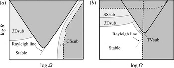
when suction is applied. The longitudinal roll-type mode studied by Taylor (Reference Taylor1923), Johnston et al. (Reference Johnston, Halleen and Lezius1972) and Min & Lueptow (Reference Min and Lueptow1994) is called the Taylor vortex (TV) mode, whilst two families of transverse-roll-type linear instabilities found in the Rayleigh-unstable and -stable parameter regions are called shear–suction (SS) and Coriolis–suction (CS) modes, respectively. For a small amount of suction, the SS and CS modes are delimited by the Rayleigh line. When the value of
 $S$
exceeds some
 $O(1)$
threshold, the linear neutral curve of the CS mode crosses the Rayleigh line whilst that of the SS mode does not. The CS mode instabilities found with increasing
 $S$
are classified as
 $\text{CS}_{I}$
and
 $\text{CS}_{II}$
modes.
When
 ${\it\Omega}=0$
, the SS mode instability corresponds to that of plane Couette flow with uniform suction. The linear stability of this flow studied by Doering et al. (Reference Doering, Spiegel and Worthing2000) is confirmed and extended to
 ${\it\Omega}>0$
in our work. The large-
 $S$
limit of the neutral curve is asymptotic suction boundary-layer flow; we also made a comparison to the linear stability studies by Hocking (Reference Hocking1975), Drazin & Reid (Reference Drazin and Reid1981) and Fransson & Alfredsson (Reference Fransson and Alfredsson2003a
) and the finite-amplitude solutions by Milinazzo & Saffman (Reference Milinazzo and Saffman1985). For transverse-roll-type two-dimensional disturbances, we found that there exists an analogy between the present rotating model and non-rotating plane Poiseuille–Couette flow subjected to uniform suction; see (2.12). The Coriolis force of the present model,
 $S{\it\Omega}$
, plays the role of pressure gradient in this analogy as shown in (2.5). For
 $R=0$
, our neutral curves of the CS mode agree with the linear stability studies of plane Poiseuille flow with uniform suction by Hains (Reference Hains1971), Sheppard (Reference Sheppard1972), Fransson & Alfredsson (Reference Fransson and Alfredsson2003b
) and Guha & Frigaard (Reference Guha and Frigaard2010). Note that our figure 8 provides a more complete stability diagram than their results. The linear instability found by GDS10 for the Rayleigh marginally stable case is essentially the
 $\text{CS}_{II}$
mode. The present work extends GDS10 to a broad parameter range including both Rayleigh-stable and -unstable cases.
Schematic of linear and subcritical instability boundaries: (a)
 $S\approx 0.4$
; (b)
 $S\approx 40$
. Thick solid, dashed and dotted curves are linear neutral curves for TV, SS and CS modes, respectively. Dark grey indicates linearly unstable region. Subcritical instabilities inferred by this study are shown by light grey; TVsub, SSsub and CSsub are the existence regions of the nonlinear solutions for the TV mode, SS mode and CS mode, respectively. The region labelled as 3Dsub indicates the existence region of the roll–streak-type three-dimensional nonlinear solutions found by Nagata (Reference Nagata1986) and Khapko et al. (Reference Khapko, Kreilos, Schlatter, Duguet, Eckhardt and Henningson2013). Thin dotted lines are the Rayleigh line.

The asymptotic studies in § 4 for large
 $R$
,
 ${\it\Omega}$
and/or
 $S$
are motivated by the numerical linear stability analyses for the full Navier–Stokes equations in § 3. A set of long-wavelength limit equations is derived for
 $S\sim O(1)$
. On the other hand, when
 $S$
is asymptotically large, the fluid layer is divided into two regions, a core layer and a wall layer. Two short-wavelength limit equations, referred to as case (i) and (ii), and a set of
 $O(1)$
wavelength equations are obtained by asymptotic reduction. The former short-wavelength cases are characterised by flow disturbances attached to the suction wall whilst in the latter
 $O(1)$
wavelength case the overall flow property is determined by the inviscid motion in the core region. We further found that the dual limits of long wavelength and large
 $S$
correspond to the two asymptotic equations by GDS10.
Now let us summarise our key results to highlight how the stability of the system changes with increasing
 $S$
and how the TV, SS and CS modes are related to these asymptotic results. As is well known, when
 $S=0$
the linear neutral curve in the
 ${\it\Omega}{-}R$
plane is that of the TV mode. When small suction is applied to the system, the
 $\text{CS}_{I}$
linear neutral curve and subcritically bifurcating finite-amplitude solutions appear. The schematic stability diagram for this suction level is pictured in figure 18(a). A notable outcome of the plane Poiseuille–Couette flow analogy is that, if there is a strong system rotation
 ${\it\Omega}$
of
 $O(S^{-1})$
, the Rayleigh-stable flow can be destabilised by asymptotically small suction. For example, for the solid-body rotation case, we observed the asymptotic linear stability threshold
 ${\it\Omega}=2\times 5772S^{-1}$
by using the analogy to the Tollmien–Schlichting-wave-type linear instability in plane Poiseuille flow without suction. The analogy also gives the saddle–node of the subcritical finite-amplitude solutions with similar
 ${\it\Omega}\sim O(S^{-1})$
scaling. This small-
 $S$
theory is only applicable when
 $R$
is sufficiently small since the Tollmien–Schlichting-wave-type linear instability disappears when the plane Couette flow component is dominant in plane Poiseuille–Couette flow without suction (Cowley & Smith Reference Cowley and Smith1985); see also appendix A.
When the small-
 $S$
asymptotic theory is not applicable, there exists a long-wavelength cut-off of the linear neutral curve at
 $S\sim O(1)$
. However, for smaller
 $O(1)$
value of
 $S$
, our analysis in § 5 suggests that a cut-off of subcritical finite-amplitude solutions exists. For example, for SS mode at
 $R=0$
, finite-amplitude solutions can be found at
 $S=1.4024$
whilst the linear neutral curve first comes into existence at
 $S=3.3511$
as shown by the long-wavelength limit analysis. For the SS and
 $\text{CS}_{I}$
modes, the corresponding linear stability cut-off value of
 $S$
is a function of the ratio
 $R/{\it\Omega}$
and recedes to infinity as the Rayleigh line is approached; see figure 14. This is consistent with the fact that the SS and
 $\text{CS}_{I}$
instabilities are separated by the Rayleigh line
 $R={\it\Omega}$
. The analysis in § 6 indicates that the bifurcation of the supercritical TV mode finite-amplitude solutions becomes subcritical at
 $S\approx 1.69$
. Both linear and nonlinear TV modes cannot cross the Rayleigh line. When
 $S\approx 22$
, the
 $\text{CS}_{II}$
mode linear neutral curve appears and then crosses the Rayleigh line. The appearance of the
 $\text{CS}_{II}$
mode is due to the long-wavelength cut-off. The supercritical bifurcation of the finite-amplitude solutions from this neutral curve is observed in § 5. The stability diagram at this stage is summarised in figure 18(b).
For asymptotically large
 $S$
, the behaviours of the SS and
 $\text{CS}_{I}$
modes are described by the case (i) short-wavelength limit, which is identical to that of asymptotic suction boundary-layer flow with the Reynolds number
 $D_{1}=S^{-1}(R-{\it\Omega})$
; see § 4.2. The results also support that these instabilities cannot exist on the Rayleigh line. By contrast, as
 $S$
increases, the
 $\text{CS}_{II}$
mode linear instability asymptotes to the inviscid limit where the critical threshold is determined by the scaled rotation rate
 ${\it\Omega}_{3}=S^{-1}{\it\Omega}$
and thus has nothing to do with the Rayleigh line; see § 4.3. Our theory and computation suggest that the asymptotic linear stability boundary of the
 $\text{CS}_{II}$
mode covers the whole linear and nonlinear
 $\text{CS}_{I}$
instabilities when
 $S$
is large. The linear critical Taylor number
 ${\it\tau}={\it\Omega}(R-{\it\Omega})$
of the TV mode is proportional to
 $S^{3}$
as
 $S\rightarrow \infty$
; see the case (ii) short-wavelength limit in § 4.2. Therefore, within the range of our research, the TV mode quickly recedes in the
 ${\it\Omega}{-}R$
plane and only the subcritical nonlinear SS and the linear
 $\text{CS}_{II}$
instabilities determine the physical stability boundary for large
 $S$
; see figures 12 and18(b).
We remark here that, in addition to the two-dimensional instabilities that we have discussed, there exist three-dimensional nonlinear instabilities with wavy longitudinal roll structures. The corresponding finite-amplitude solutions were discovered by Nagata (Reference Nagata1986) for rotating plane Couette flow without suction and by Khapko et al. (Reference Khapko, Kreilos, Schlatter, Duguet, Eckhardt and Henningson2013) for asymptotic suction boundary-layer flow. The study of Rincon, Ogilvie & Cossu (Reference Rincon, Ogilvie and Cossu2007) shows these wavy solutions cannot cross the Rayleigh line. Also, the known fully nonlinear three-dimensional asymptotic theories are not applicable for large
 ${\it\Omega}$
. For example, the vortex–wave interaction theory by Hall & Smith (Reference Hall and Smith1991) and Hall & Sherwin (Reference Hall and Sherwin2010) is not valid when
 ${\it\Omega}$
becomes larger than
 $O(R^{-1})$
, whilst the free-stream coherent structure theory by Deguchi & Hall (Reference Deguchi and Hall2014) breaks down at
 ${\it\Omega}\gtrsim O(1)$
. The existence region of these three-dimensional instabilities is also pictured in figure 18. One of the alternative candidates for three-dimensional instability in the Rayleigh-stable parameter region is finite-amplitude solutions bifurcating from the SS or CS mode solutions. These types of solutions are free from the Poiseuille–Couette flow analogy and thus may invade the linearly and nonlinearly stable parameter regions derived in this paper. Connections of the present work to recently found three-dimensional travelling waves in Rayleigh-stable Taylor–Couette flow by Deguchi, Meseguer & Mellibovsky (Reference Deguchi, Meseguer and Mellibovsky2014) is also of interest.
Variation of the cut-off suction level
 $S_{0c}$
as a function of (a)
 ${\it\Omega}_{0}$
, (b)
 $D_{0}$
and (c)
 $D_{0}/{\it\Omega}_{0}$
along the curve traced in figure 14 for
 $\arctan (R_{0}/{\it\Omega}_{0})\in [{\rm\pi}/4,{\rm\pi}/2]$
. The solid and dashed lines correspond to the
 $\text{CS}_{II}$
and SS modes, respectively. The asymptotic lines indicated by thin dotted lines are given by the optimal values in figure 21. (d) The same as panel (b) but for
 $\arctan (R_{0}/{\it\Omega}_{0})\in [0,{\rm\pi}/4]$
and smaller value of
 $S_{0c}$
. The dotted line in this panel is determined from the long-wavelength cut-off parameter value of plane Poiseuille–Couette flow problem by Cowley & Smith (Reference Cowley and Smith1985).

As shown in figure 18, we found
 $\text{CS}_{I}$
and
 $\text{CS}_{II}$
instabilities in Rayleigh-stable flow, including Keplerian motion
 ${\it\Omega}={\textstyle \frac{2}{3}}R$
, which any orbiting material under central gravitational force obeys. Therefore, the present study is considered to increase the likelihood of hydrodynamic instability in a cold accretion disk. Our theory may be applicable if we assume that the orbiting material interacts and behaves as a continuum. The rotation rate and suction effect, created by the gravitational force and by the mass loss at the edge of the black hole, respectively, may be responsible for the suction–shear–Coriolis instability in the Keplerian flow.
Acknowledgements
K.D. would like to acknowledge Dr A. H. White for his helpful comments and all the authors wish to thank the anonymous referees for their valuable comments that have improved the initial manuscript.
Appendix A. The dual limits of large suction and long wavelength
Near the blow-up points at
 $\arctan (R_{0}/{\it\Omega}_{0})\approx {\rm\pi}/4$
and
 ${\rm\pi}/2$
in figure 14, we can find asymptotic behaviours as pictured in figure 19(a,b), where the curves in figure 14 are plotted as a function of
 $D_{0}=R_{0}-{\it\Omega}_{0}$
and
 ${\it\Omega}_{0}$
. Note that the parameter range is restricted to
 $\arctan (R_{0}/{\it\Omega}_{0})\in [{\rm\pi}/4,{\rm\pi}/2]$
for the sake of simplicity. Here we analyse these asymptotic behaviours, which correspond to dual limits of long wavelength and large suction.
Visualisations of the neutral disturbances in terms of stream function (left; the definitions of solid and dotted lines are the same as in figure 5) and eigenfunction
 ${\it\Phi}$
(right; the solid line represents the real part whilst the dashed line represents the imaginary part): (a) the SS mode at
 $(S,{\it\Omega}_{0},D_{0})=(100,1.51\times 10^{9},4.09\times 10^{7})$
; (b) the
 $\text{CS}_{II}$
mode at
 $(S,{\it\Omega}_{0},D_{0})=(30,628,2.09\times 10^{8})$
.

At
 $\arctan (R_{0}/{\it\Omega}_{0c})\approx {\rm\pi}/4$
in figure 14, where the cut-off curve of the SS mode blows up,
 $D_{0}$
and
 ${\it\Omega}_{0}$
are proportional to
 $S^{2}$
and
 $S^{3}$
, respectively. Adopting the scaling
 $[{\it\Omega}_{4},D_{4},s]\rightarrow [S^{-3}{\it\Omega}_{0},S^{-2}D_{0},S^{-2}(s+2\text{i}D_{0})]$
in (5.8), we find distinct structures in the core, upper wall layer and lower wall layer. In the core layer, we find that the leading-order equation satisfies
 ${\it\Phi}^{\prime \prime }=0$
and therefore
 ${\it\Phi}$
must have a linear profile, as can be confirmed in the visualisation of the corresponding full Navier–Stokes neutral mode shown in figure 20(a). The thin upper and lower wall layers adjust the fluid motion to the no-slip boundary conditions. In the upper wall layer, where
 $Y=S^{3/2}(1-y)\sim O(1)$
and the viscous effect is recovered, the leading-order equation
 $$\begin{eqnarray}\left(2{\it\Omega}_{4}-\frac{\text{d}^{2}}{\text{d}Y^{2}}\right)\frac{\text{d}^{2}{\it\Phi}}{\text{d}Y^{2}}=0\end{eqnarray}$$
has a solution
 ${\it\Phi}=S^{-3/2}\{Y+(\text{e}^{-\sqrt{2{\it\Omega}_{4}}Y}-1)/\sqrt{2{\it\Omega}_{4}}\}$
. This solution satisfies the no-slip boundary conditions on the upper wall and the matching condition to the core solution
 ${\it\Phi}=(1-y)$
as
 $Y\rightarrow \infty$
. The linear stability is determined by the lower wall layer where
 $Y=S(1+y)\sim O(1)$
and the leading-order equation is
 $$\begin{eqnarray}\left(\left(s+\text{i}({\it\Omega}_{4}Y-2D_{4}\text{e}^{-Y})-\frac{\text{d}}{\text{d}Y}\right)\frac{\text{d}^{2}}{\text{d}Y^{2}}+2\text{i}D_{4}\text{e}^{-Y}-\frac{\text{d}^{4}}{\text{d}Y^{4}}\right){\it\Phi}=0.\end{eqnarray}$$
In order to match the core solution, the boundary conditions
 $$\begin{eqnarray}\left.\begin{array}{@{}ll@{}}{\it\Phi}={\it\Phi}^{\prime }=0 & \quad \text{at}\ Y=0,\\ {\it\Phi}^{\prime }={\it\Phi}^{\prime \prime }=0 & \quad \text{at}\ Y=\infty ,\end{array}\right\}\end{eqnarray}$$
must be satisfied. This dual limit problem (A 2) is successfully solved by using mapping (5.4) and the basis
 $$\begin{eqnarray}{\it\Phi}_{l}({\it\eta})=(1-{\it\eta}^{2})^{2}T_{l}({\it\eta})+{\textstyle \frac{4}{3}}({\it\eta}+1)^{2}({\it\eta}-2).\end{eqnarray}$$
The numerically solved neutral curve of (A 2) is shown in figure 21(a). The critical values
 $({\it\Omega}_{4c},D_{4c})=(1536,4007)$
, which can be obtained by minimising the ratio
 $D_{4}/{\it\Omega}_{4}$
along the stability curve, describe the blow-up behaviour of the dashed line in figure 14. Note that
 $(D_{0}/{\it\Omega}_{0})\ll 1$
means
 $\arctan (R_{0}/{\it\Omega}_{0})\approx {\rm\pi}/4$
. The optimised values indeed give the asymptotic line
 $(D_{0}/{\it\Omega}_{0})=(D_{4c}/{\it\Omega}_{4c})S_{0c}^{-1}$
in figure 19(c).
(a) The stability of dual asymptotic problem (A 2) where the optimal values indicated by the arrow are
 $({\it\Omega}_{4c},D_{4c})=(1536,4007)$
. (b) Similar plot to panel (a) but for the problem (A 5). The inset is the close-up of the tip of the neutral curve which determines the optimal values
 $({\it\Omega}_{5c},D_{5c})=(0.0232,2.03\times 10^{-21})$
indicated by the arrow. The thin dotted line corresponds to the asymptotic analysis by GDS10. The range of truncation level used in the computation is
 $L\in [60,100]$
.

A similar analysis can be performed for the blow-up point of the cut-off curves of the
 $\text{CS}_{II}$
mode at
 $\arctan (R_{0}/{\it\Omega}_{0})\approx {\rm\pi}/2$
. The scaling
 $[{\it\Omega}_{5},D_{5},s]\rightarrow [\!S^{-3}{\it\Omega}_{0},S^{-2}\text{e}^{-2S}D_{0},$
 $S^{-2}(s-2\text{i}D_{0}-2\text{i}{\it\Omega}_{0})\!]$
is assumed in view of figure 19(a,b). The leading-order dynamics is governed by
 $$\begin{eqnarray}\left(\left(s-\text{i}({\it\Omega}_{5}Y+2D_{5}\text{e}^{Y})+\frac{\text{d}}{\text{d}Y}\right)\frac{\text{d}^{2}}{\text{d}Y^{2}}+2\text{i}D_{5}\text{e}^{Y}-\frac{\text{d}^{4}}{\text{d}Y^{4}}\right){\it\Phi}=0,\end{eqnarray}$$
with boundary conditions
 $$\begin{eqnarray}{\it\Phi}={\it\Phi}^{\prime }=0\quad \text{at}\ Y=0,\infty\end{eqnarray}$$
in the upper wall layer, where
 $Y=S(1-y)\sim O(1)$
. Note that when the terms including
 $D_{5}\text{e}^{Y}$
are dominant, i.e.
 $Y$
is larger than
 $-\ln (D_{5})\approx -0.588$
,
 ${\it\Phi}$
decays to zero exponentially towards the boundary as shown in figure 20(b). The mapping technique (5.4) does not work for the dual limit problem (A 5) since the exponential decay of the solution leads to an ill-conditioned matrix in the linear algebraic problem. This difficulty could be overcome by posing the boundary conditions (A 6) at
 $Y=Y_{q}\equiv -\ln (qD_{5})>1$
(i.e.
 $q<1$
), instead of
 $Y\rightarrow \infty$
. The smaller the value of
 $q$
, the better the approximation. The interval
 $Y\in [0,Y_{q}]$
is mapped to
 ${\it\eta}=2Y/Y_{q}-1\in [-1,1]$
to use the basis function (5.7). The range of parameter
 $q$
is chosen as 0.0001–0.00002 by trial and error. By minimising the ratio
 ${\it\Omega}_{5}/D_{5}$
along the numerically solved neutral curve in figure 21(b), we have the optimal parameter values
 $({\it\Omega}_{5c},D_{5c})=(0.0232,2.03\times 10^{-21})$
, which determine the asymptotic line
 $({\it\Omega}_{0}/D_{0})=({\it\Omega}_{5c}/D_{5c})S\,\text{e}^{-2S}$
in figure 19(c).
The blow-up behaviour of the dashed line at
 $\arctan (R_{0}/{\it\Omega}_{0})\approx 0.03{\rm\pi}$
in figure 14 is not caused by its asymptotic nature. In the vicinity of this irregular point, we confirm that the neutral curve in the
 $S{-}R_{0}$
parameter plane (figure 13), which defines
 $S_{0c}$
, forms a loop and shrinks to a point as the irregular point is approached.
All of the calculations here are spanwise independent and therefore it is possible to compare with the results of plane Poiseuille–Couette flow with uniform suction; see (2.12). Our result is consistent with the recent investigation on the long-wavelength cut-off values of the flow configuration in Guha & Frigaard (Reference Guha and Frigaard2010) and earlier in Nicoud & Angilella (Reference Nicoud and Angilella1997).
Recalling the remark just below (2.7), we can apply the result of plane Poiseuille–Couette flow by Cowley & Smith (Reference Cowley and Smith1985) when
 $S$
is small. According to their results, Tollmien–Schlichting-wave-type linear instability of this flow experiences a long-wavelength cut-off when
 $|R_{PCF}/R_{PPF}|\approx 0.352$
and
 $|{\it\alpha}R_{PPF}|\approx 7156.5$
with increasing
 $R_{PCF}$
. This result is relevant to the small-
 $S$
behaviour of the cut-off curve of the SS mode in the vicinity of
 $\arctan (R_{0}/{\it\Omega}_{0})\approx 0$
. In figure 19(d), where the
 $D{-}S_{0c}$
diagram of the cut-off threshold is plotted for
 $\arctan (R_{0}/{\it\Omega}_{0})\in [0,{\rm\pi}/4]$
, we can see that the curve is asymptotic to the line
 $D_{0}S_{0}/2=7156.5$
. The necessary condition for the Tollmien–Schlichting-wave-type instability,
 $R_{PCF}\lesssim 0.352R_{PPF}$
, implies that, in order to create the small-
 $S$
asymptotic theory seen in figure 8, where
 ${\it\Omega}\sim O(S^{-1})$
,
 $R$
must be of
 $O(1)$
value or less. Therefore, except for
 $\arctan (R/{\it\Omega})\ll 1$
, there is a long-wavelength cut-off at finite
 $S$
.