





1. Introduction
Recently, a new discussion has been sparked regarding a phenomenon in turbulent jets referred to as ‘guided jet waves’ and ‘trapped waves’, with notable repercussions for jet far-field noise prediction in the forward-flight direction. The waves, originally identified by Tam & Hu (Reference Tam and Hu1989) as upstream-travelling neutral waves within the framework of the vortex sheet model, occur in specific frequency and wavenumber bands, and can be classified into modes identified by their azimuthal and radial structure. The signature of the trapped waves manifest as a series of tones in the near- and far-field spectra at the upstream angles. Given most anechoic facilities are not equipped to measure the far-field noise in the forward-flight angles, this phenomenon has been overlooked for a long time (Zaman et al. Reference Zaman, Bridges, Upadhyay and Brown2024). However, the last few years have seen a flurry of research interest focused towards understanding the properties of guided and trapped waves and the conditions under which they exist (Towne et al. Reference Towne, Cavalieri, Jordan, Colonius, Schmidt, Jaunet and Brès2017; Martini, Cavalieri & Jordan Reference Martini, Cavalieri and Jordan2019; Nogueira et al. Reference Nogueira, Cavalieri, Martini, Towne, Jordan and Edgington-Mitchell2024; Bogey Reference Bogey2025), and measuring their acoustic footprint in the far-field (Bogey Reference Bogey2022; Zaman Reference Zaman2023; Zaman et al. Reference Zaman, Bridges, Upadhyay and Brown2024). Furthermore, the role of upstream-travelling guided jet waves in the feedback that forms the basis for resonant tones in screeching (Shen & Tam Reference Shen and Tam2002; Edgington-Mitchell et al. 2018, 2022; Mancinelli et al. 2019, 2021) and impinging jets (Tam & Ahuja Reference Tam and Ahuja1990; Bogey & Gojon Reference Bogey and Gojon2017) has also been investigated. Trapped waves may also have engineering relevance in engine integration applications, potentially playing roles in multi-stream internally mixed nozzles (Ramsey, Mayo & Ahuja Reference Ramsey, Mayo and Ahuja2023), jet–airframe integration (Zaman et al. Reference Zaman, Fagan, Bridges and Brown2015; Tam & Chandramouli Reference Tam and Chandramouli2020) and other conditions where a high-speed jet–surface interaction can occur, such as a jet–flap interaction (Jordan et al. Reference Jordan, Jaunet, Towne, Cavalieri, Colonius, Schmidt and Agarwal2018).
The first comprehensive experimental documentation of the near-field acoustic signature of the guided jet waves in circular and rectangular nozzles was provided by Zaman, Fagan & Upadhyay (Reference Zaman, Fagan and Upadhyay2022). They subsequently demonstrated that the series of spectral tones observed in the near-field persist in the acoustic far-field in the upstream, forward-flight angles for cold and heated jets for a range of high-subsonic, and ideally and non-ideally expanded supersonic Mach numbers (Zaman et al. Reference Zaman, Bridges, Upadhyay and Brown2024). It was shown that the peaks for the rectangular nozzles appear as an integer harmonic series, whereas the tones for circular jets appeared to form a fractional series of the form
 $f_n=f_1(2n+1)/3$
(i.e. 5/3, 7/3, 9/3, etc.). Further, the spectral peaks at subsonic Mach numbers are smoothly continued in the supersonic regime as screech tones, providing additional context that the phenomena of trapped waves and screech must be connected (see figure 9 of Zaman et al. Reference Zaman, Bridges, Upadhyay and Brown2024, where tone frequencies at subsonic Mach numbers continue as screech tones when the jet becomes supersonic).
The discussion on trapped waves, initiated by Towne et al. (Reference Towne, Cavalieri, Jordan, Colonius, Jaunet, Schmidt and Brès2016, Reference Towne, Cavalieri, Jordan, Colonius, Schmidt, Jaunet and Brès2017) as theory development and Jaunet et al. (Reference Jaunet, Jordan, Cavalieri, Towne, Colonius, Schmidt and Brès2016) as an initial supporting experimental evidence, stems from the ‘soft duct’ solution of the Helmholtz equation applied to the inner stream of the jet, in contrast with the ‘vortex sheet’ solution studied by Michalke (Reference Michalke1970), Tam (Reference Tam1971) and Tam & Hu (Reference Tam and Hu1989), which considers both inner and outer streams. Under this framework, the jet is simplified to a soft duct with a pressure-release boundary condition at the wall, and the supported waves are of acoustic nature. For high subsonic Mach numbers, it was shown that both upstream- and downstream-propagating waves can exist in the jet core and, depending on the frequency and spatial wavenumber, are either fully confined within the jet core or partly transmitted through the shear layer, propagating as free stream acoustic waves in the ambient. The waves of opposing group velocities may exchange energy at the nozzle lip and a downstream turning point caused by the contraction of the potential core, potentially resulting in resonance (Towne et al. Reference Towne, Cavalieri, Jordan, Colonius, Schmidt, Jaunet and Brès2017). Schmidt et al. (Reference Schmidt, Towne, Colonius, Cavalieri, Jordan and Brès2017) further observed, in their large-eddy simulation (LES) studies of an
 $M_{\!j}=0.9$
,
 $T_{\!j}/T_\infty =1$
jet, the presence of upstream-travelling trapped waves that match the vortex sheet mode using cross-spectral density matrix analysis. Building upon these observations, Martini et al. (Reference Martini, Cavalieri and Jordan2019) provided further physical insight by observing that the vortex-sheet impedance can provide a soft- or hard-walled duct boundary to the trapped waves in limiting cases depending on whether the shear layer defines a jet or a wake, and whether the jet/wake is hotter or colder than the outer stream. Their work generalises the prediction of trapped waves to wakes and other propulsive conditions that may involve co-flow. Most recently, Nogueira et al. (Reference Nogueira, Cavalieri, Martini, Towne, Jordan and Edgington-Mitchell2024) clarified the fundamental mechanism underlying guided jet modes by showing that the acoustic waves generated within the core of the jet can undergo internal reflection and/or transmission at the shear layer depending on their frequency, wavenumber and wave angle with respect to the jet axis. Because the shear layer can be thought of as an impedance mismatch between two domains (inside and outside the jet), there are certain angles for which a total internal reflection of the waves generated within the jet is possible, making the jet behave as an acoustic waveguide for both upstream- and downstream-travelling disturbances. The discrete streamwise wavenumbers are dictated by the requirement that the radial modes defining the waves must fit within the jet shear layer (Nogueira et al. Reference Nogueira, Cavalieri, Martini, Towne, Jordan and Edgington-Mitchell2024). These findings are also supported by Bogey (Reference Bogey2025), with both works hypothesising that the transmission to the ambient is maximum for wavenumbers close to the sonic line of the ambient stream, with the transmission coefficient rapidly decreasing as the waves become increasingly more subsonic, resulting in modes that are confined within the jet.
Sketches of the dispersion diagrams for the different wave solutions to the vortex sheet problem from Tam & Hu (Reference Tam and Hu1989) at different Mach number ranges. Groups
 $\unicode {x2460}$
,
 $\unicode {x2461}$
, ‘Trapped Waves’; Group
 $\unicode {x2462}$
, ‘Guided Jet Waves’.

In other comprehensive investigations of trapped waves, careful examination has been performed in the LES by Bogey (Reference Bogey2021), showing that the modes for the guided jet wave peaks match the vortex sheet predictions of Tam & Hu (Reference Tam and Hu1989) for a wide range of Mach numbers in the range of
 $0.5\lt M_a \lt 2$
, where the supersonic cases operate as nearly ideally expanded. Near-field spectral tones due to guided jet waves with non-negligible radial support are shown to match experimental measurements and persist in the far-field (Bogey Reference Bogey2022). Further experimental evidence was provided by Edgington-Mitchell et al. (Reference Edgington-Mitchell, Weightman, Mazharmanesh and Nogueira2025), who used schlieren to visualise a trapped, upstream-propagating shock originating from the interaction of a subsonic jet with a flat plate at
 $0.85\lt M_{\!j}\lt 0.9$
, constituting the strongest experimental evidence to date of the existence of trapped waves in the jet core – although in their impinging jet case, these waves seem to coalesce into an upstream-travelling shock.
As well summarised by Ramsey (Reference Ramsey2024), the vortex sheet model of Tam & Hu (Reference Tam and Hu1989) has two categories of waves with upstream phase velocity. The so-called ‘trapped waves’ refer to the family of solutions of the vortex sheet dispersion relationship that contains large pressure fluctuations only within the jet core and very closely match the ‘soft duct’ model with the pressure-release boundary condition. However, the ‘guided jet waves’ would also be part of the same dispersion relationship for the same mode shape category (i.e. axisymmetric or helical), but would comprise waves with upstream phase velocities for which the pressure fluctuation contains a non-negligible value outside of the jet core. The transition between ‘trapped waves’ and ‘guided jet waves’ is smooth, and an increasingly larger pressure fluctuation is observed outside of the potential core of the jet as the ‘trapped waves’ wavenumber decreases and approaches the ‘guided waves’, which have the lowest wavenumbers of the group. Represented schematically in figure 1, we provide three sketches of the generic shapes for wave solutions supported by the vortex sheet model of Tam & Hu (Reference Tam and Hu1989) at different relevant Mach number ranges on a dispersion diagram, showing the neutral waves of the form
 \begin{equation} P^\prime (x,r,\theta ,t) = P_0^\prime (r) \textrm{e}^{\textrm{i}(\omega t-kx+m\theta )} \end{equation}
for a typical vortex sheet solution as a blue line. We limit figure 1 to displaying the upstream phase velocity waves located at negative
 $k$
and positive
 $\omega$
. The dashed bounds
 $u_{\!j}-a_{\!j}$
(green) and
 $-a_\infty$
(red) are the upstream-propagating sound speeds inside and outside the jet, respectively. We group the waves into three groups. The waves in Group
 $\unicode {x2460}$
are directed upstream, with upstream phase velocity (
 $\omega /k$
negative) and group velocity (
 $\partial \omega /\partial k$
also negative). These waves correspond to ‘trapped waves’, i.e. waves with non-negligible pressure fluctuations
 $P^\prime (r)$
only inside the jet core. Group
 $\unicode {x2461}$
waves are also ‘trapped waves’ that have upstream phase velocity, but downstream group velocity and have small but non-negligible pressure fluctuations outside the jet core, but the maximum fluctuation still occurs inside the jet core. These waves only occur in the transonic range in figure 1(b). Waves in Group
 $\unicode {x2462}$
have both upstream phase and group velocity, and consist of ‘guided waves’ with large pressure fluctuations both inside the jet core and also outside the jet. Although we choose the bounds at the points of zero group velocity to highlight the change in energy propagation direction, the transition between ‘trapped waves’ and ‘guided waves’ is smooth, with the ‘trapped waves’ finding an increasingly larger fluctuation outside of the jet as their wavenumber
 $|k|$
decreases.
When comparing figure 1(a,b) with figure 1(c), it is clear that the ‘trapped wave’ of Group
 $\unicode {x2460}$
, which has upstream group velocity, exists only for subsonic jets, and therefore a feedback loop through the ‘trapped waves’ mode could only be possible in subsonic jets, even if such upstream phase velocity waves also may appear to exist in the supersonic regime. More importantly, to establish the speed at which information is propagated with reference to the ambient speed of sound, the analysis of multiple wavenumber/frequency pairs is required to establish the group velocity
 $v_g=\partial \omega /\partial k$
. Experimentally, this requires time-resolved imaging.
For transonic jets shown in figure 1(b) at
 $0.8\lt M_{\!j}\lt 1$
, there are two wave groups with upstream group velocity (Groups
 $\unicode {x2460}$
and
 $\unicode {x2462}$
), transferring energy upstream. Similarly, energy can be transferred downstream by waves of Group
 $\unicode {x2461}$
and also the Kelvin–Helmholtz instability waves (not shown in figure 1). Thus, if a feedback mechanism exists transferring energy back-and-forth between different streamwise locations in the jet, it must involve one of the four possible pairings {
 $\unicode {x2460}$
,
 $\unicode {x2461}$
}; {
 $\unicode {x2462}$
,
 $\unicode {x2461}$
};
 or
 . For supersonic jets, the trapped waves from Group
 $\unicode {x2460}$
cease to exist, and the only possible pairings are {
 $\unicode {x2462}$
,
 $\unicode {x2461}$
} and
 . Prinja et al. (Reference Prinja, Martini, Jordan, Towne and Cavalieri2024) postulate in their analysis of LES data of a
 $M_{\!j}=M_a=0.9$
jet (only mode (0, 1) is analysed) that group pairings {
 $\unicode {x2460}$
,
 $\unicode {x2461}$
} and {
 $\unicode {x2462}$
,
 $\unicode {x2461}$
} are active and have high reflection coefficient at certain turning point locations, whereas the
 group has low reflection coefficient throughout. However, a mechanism for radiation of acoustic waves with higher intensity at certain frequencies is yet to be clarified.
This work will demonstrate, through analysis of time-resolved schlieren images at high-subsonic Mach numbers where shocks do not dominate the images, that a series of upstream phase and group velocity waves exists inside of the jet. We also explore the shape of the trapped wave packets through spectral proper orthogonal decomposition (POD), their relationship with the theoretical predictions from vortex-sheet modes and also our observations that these wavepackets are detected for chevron nozzles, potentially indicating that any possible feedback loop responsible for observed spectral peaks in the acoustic far-field (Zaman et al. Reference Zaman, Bridges, Upadhyay and Brown2024) do not depend on azimuthally uniform impedance boundary condition at the nozzle lip.
(a) Photograph of the SAFS set-up at the CW-17 facility with one of our chevron nozzles mounted. (b) Schematic of the SAFS system optical set-up. LPV, linear polariser (Vertical); LPH, linear polariser (horizontal); RR, Ronchi ruling; WP, Wollaston prism;
 $\lambda /4$
, quarter-wave plate.

2. Methods
2.1. Facility and nozzles
The majority of the results reported herein will be derived from experiments performed at the CW-17 open jet facility at NASA Glenn Research Center. In the CW-17 facility, compressed air passes through a 30 inch diameter plenum and discharges through the nozzle into the quiescent ambient of the test cell. The plenum is fitted with a bell-mouth with 5.16 inch exit diameter and a 17.8
 $^\circ$
wall slope. A conical adapter with a 2.558 inch exit attaches to the bellmouth and allows interchangeable mounting of various nozzles. A condition was achieved using a Sensotec pressure transducer calibrated to an uncertainty of
 $\pm 0.09\,\%$
with respect to the full scale of 50 psig, resulting in an uncertainty in the NPR of
 $\pm 0.003$
. A photograph of the test cell where the self-aligning focusing schlieren (SAFS) was performed is shown in figure 2(a).
The select acoustic spectra presented herein were acquired as a part of a different test campaign on the Small Hot Jet Acoustic Rig (SHJAR) at NASA GRC. The SHJAR is housed within the Aeroacoustic Propulsion Lab (AAPL), a 65 ft radius geodesic hemispherical dome lined with anechoic wedges, with a cutoff frequency of 200 Hz (Bridges & Wernet Reference Bridges and Wernet2012). The details of the experimental effort to acquire far-field microphone data, including in the jet forward flight angles and the prominence of an acoustic signature that could be associated with the trapped waves in the acoustic far-field are discussed by Zaman et al. (Reference Zaman, Bridges, Upadhyay and Brown2024). Some of the near-field microphone measurements presented are from CW-17. It should be noted that CW-17 is not an anechoic facility and the corresponding acoustic data are only used for clarification of the observations when data from SHJAR are not available. To further clarify which data are available for each condition, table 1 is provided; noting that whenever microphone data from SHJAR were available, these were prioritised in our analysis.
Experimental test conditions examined in this manuscript. All nozzles are convergent. NF = near-field microphones; FF = far-field microphones; SAFS = self-aligning focusing schlieren.

Table 1. Long description
A table comparing experimental test conditions for different nozzles. The table has 6 rows and 10 columns. Column headers are Nozzle, M j, M a, T j/T∞, D j [mm], u j [m s⁻¹], ReD, knyD, Stny, and CW-17 data SHJAR data. Row 1: Conical 1.5°, 0.9, 0.835, 0.861, 38.1, 288.9, 8.5 x 10, 448.3, 2.64, SAFS+NF. Row 2: Conical 1.5°, 0.983, 0.9, 0.838, 38.1, 311.4, 9.4 x 10, 448.3, 2.45, SAFS+NF. Row 3: SMC000 2″, 0.9, 0.835, 0.861, 50.8, 288.9, 1.1 x 10, 597.7, 3.26, SAFS, NF+FF. Row 4: SMC000 2″, 0.983, 0.9, 0.838, 50.8, 311.4, 1.3 x 10, 597.7, 3.52, SAFS, NF+FF. Row 5: SMC001, 0.9, 0.835, 0.861, 50.8, 288.9, 1.1 x 10, —, —, SAFS. The table compares different nozzles and their respective experimental conditions, including Mach numbers, temperature ratios, diameters, velocities, Reynolds numbers, and specific data types.
In the SHJAR facility, microphone measurements are acquired using Hottinger Brüel and Kjaer (HBK) microphones (model B&K 4939) with LAN-XI signal conditioning, and data acquisition hardware and Tescia software. The data were acquired at a sampling rate of 262 144 samples per second with a high-pass filter at 22.4 Hz and a low-pass filter set at 102.4 kHz. In CW-17, microphone measurements were acquired using B&K 4135 microphones at a sampling rate of 100 kHz with a 50 kHz low-pass filter.
Observations pertaining to three nozzles will be discussed in this manuscript: SMC000 (
 $D=2''$
), SMC001 (nominal
 $D=2''$
) and Conical (
 $D=1.5''$
) nozzle. The nozzles are displayed in figure 3 along with relevant dimensions. The nozzle geometries, along with the rationale for their choice, are further described by Bridges & Brown (Reference Bridges and Brown2004). The SMC000 and Conical
 $1.5''$
nozzles are both convergent conical 5
 $^\circ$
nozzles and both produce a traditional axisymmetric circular jet; but the diameters of the nozzles are different, leading to different physical frequencies that will aid us in ascertaining the phenomena observed are not artifacts of our acquisition system. Further, the two nozzles have different contours, mostly because the nozzle mount was designed to accommodate the SMC000
 $2''$
nozzle conical contour; and to reach the
 $1.5''$
exit diameter over the same streamwise exit plane, the Conical
 $1.5''$
nozzle has a curved region with a 19 mm radius step connecting the two different diameters inside the nozzle, as shown in figure 3. Although the exit angles of the two circular nozzles are the same, we keep the SMC000 nomenclature for the
 $2''$
nozzle to facilitate referencing to previous works.
The SMC001 nozzle, however, contains six chevrons cut into the SMC000 nozzle shape. There is no change in the internal conical profile for the SMC001 nozzle, so it is regarded as a ‘penetrating’ chevron as the petals continue converging with the 5
 $^\circ$
cone angle. The addition of chevrons, as observed by Bridges & Brown (Reference Bridges and Brown2004), shifts the noise spectrum towards higher frequencies, presenting an improvement in low-frequency noise at the detriment of high-frequency noise. Chevrons also reduce noise in the downstream angles, while increasing noise at the upstream angles. Crucially, we present this case to examine the effect of the serrations, which change the nozzle lip boundary condition and potentially could disrupt a feedback loop if a feedback mechanism with the nozzle lip is responsible for the noise emission related to these trapped waves.
Photographs and drawings containing the main dimensions of the nozzles used in this study. SMC nozzle photographs taken from Bridges & Brown (Reference Bridges and Brown2004).

Figure 3. Long description
The image contains three photos and two diagrams. Panel A and Panel B show photographs of two different SMC series nozzles with a 2-inch exit diameter. Panel C shows a photograph of a conical nozzle with a 1.5-inch exit diameter. Panel D and Panel E are diagrams illustrating the main dimensions of the SMC series nozzles and the conical nozzle, respectively. The diagrams include labels for the exit diameters and angles.
2.2. Self-aligned focusing schlieren
To acquire the images discussed in this work, a time-resolved self-aligning focusing schlieren (SAFS) system, developed initially by Bathel & Weisberger (Reference Bathel and Weisberger2022) and further described by Page et al. (Reference Page, Boyda, Fahringer, Weisberger, Bathel, Wernet and Heineck2025), was employed. A schematic of the optical train used is presented in figure 2(b). One notable difference in our SAFS system is that we employ wire-grid linear polarisers and instead of a polarisation beam splitting cube, the third wire-grid polariser is used to polarise and turn the light source beam down the axis of the SAFS system. The advantage of the SAFS system is its portability, as the optical system can be easily moved across facilities without the necessity for highly rigid mirror mounts or their alignment, being ideal to service the multiple facilities at GRC. The SAFS system was configured to provide an
 $8''$
wide field of view along the axis of the jet, encompassing approximately 5 nozzle diameters. A Photron SA-Z camera, equipped with 128 GB of RAM and sampling at 40 000 fps, captured the images formed in the SAFS optical train through a relay lens at a resolution of 1024
 $\times$
512 px.
The focusing schlieren optical train works by projecting the 20 line pairs mm−1 Ronchi ruling onto the jet schlieren object by using the Cavilux laser as a light source exposing the schlieren object for a 30 nanosecond pulse duration. The Cavilux laser light passes through a vertical linear polariser and is reflected through the plate beam splitter (another vertical polariser) into the flow domain. The light goes through the Ronchi ruling and through a glass/quartz Wollaston prism with a 7.5 arc-minute deviation angle towards the field lens, which focuses the image of the Ronchi ruling onto the retroreflective background at the opposite side of the jet. The quarter-wave plate (
 $\lambda /4$
) turns the linearly polarised light into right-handed circularly polarised light. When the light goes through the schlieren object and is reflected back from the retroreflective background, its circular polarisation handedness is flipped to left-handed circularly polarised light such that when it passes through the quarter-wave plate again, it will be delayed into horizontal linearly polarised light, which is perpendicular to the outgoing light. Only horizontally polarised light is permitted to enter the camera through the horizontal polariser and the relay lens, providing discrimination from the outgoing vertical linearly polarised light. The Wollaston prism is then able to provide a small angular shift to the oncoming beam, which is then cut off by the same Ronchi ruling without requiring any alignment as the grid automatically has a matching conjugate plane at its mirror image by construction. In our SAFS system, the field lens image focal plane sits inside the optical train and therefore a relay lens needs to be placed between the camera sensor and the beam splitter to properly image the jet. A relay lens and a set of extension tubes were required, as the conjugate plane to the schlieren object was located in front of the Ronchi ruling.
As a focusing schlieren system, we hoped that it would provide a sufficiently narrow depth of field to isolate turbulent features inside the core of our jets and exclude features from the shear layers along the optical axis. However, due to the large field of view required for this study, the depth of field was found to exceed the jet diameter and the images should be treated as traditional schlieren images. Further details on empirical estimation of the schlieren depth of field are provided in Appendix B.
To extract any coherent behaviour observed in the images acquired, the raw time-resolved SAFS images were processed using the spectral POD (SPOD) algorithm open-sourced by Towne, Schmidt & Colonius (Reference Towne, Schmidt and Colonius2018). The technique allows the estimation of the eigenvalues and eigenvectors of the cross-spectral density matrix based on measurement data (Schmidt & Colonius Reference Schmidt and Colonius2020), and correspond to an extension of the Welch periodogram method to multiple concurrent, simultaneously-acquired sensor signals such as the pixels of a high-speed camera. A mode shape is obtained for each frequency computed, encoding the relative amplitude and phase relationships through a spatial map of complex numbers for a given frequency. These modes then indicate the spatial distributions of the waves observed from the image data, as well as their direction of propagation. The reader is directed to Taira et al. (Reference Taira, Brunton, Dawson, Rowley, Colonius, McKeon, Schmidt, Gordeyev, Theofilis and Ukeiley2017) and Schmidt & Colonius (Reference Schmidt and Colonius2020) for a detailed explanation of the SPOD algorithm, its interpretation and its relationship to other modal analysis techniques.
Note, however, that the SPOD modes extracted will be biased by the type of data available for processing – in this case, the line-integrated, streamwise density gradient
 $\partial \rho /\partial x$
. Therefore, we expect the eigenvalue spectra obtained to be biased towards higher wavenumbers, since the energy norm is based only on the derivative
 $\partial \rho /\partial x \sim k_x$
. Since we are examining dispersive waves in this work, the inherent single-frequency analysis nature of SPOD will accentuate higher wavenumber content for a given temporal frequency, if any high wavenumber structure is present. Therefore, the spectral slopes do not have as much interpretability as if the waves present in the flow were non-dispersive.
The images analysed were captured at
 $f_s=40\,\text{kHz}$
, and SPOD processing was done with
 $N_{\textit{fft}}=2048$
,
 $N_{\textit{blk}}=508$
on the 261 831 images (
 ${\sim} 6.55$
s) acquired for the SMC000 and SMC001 nozzles; and
 $N_{\textit{fft}}=2048$
,
 $N_{\textit{blk}}=252$
on the 130 765 images (
 ${\sim} 3.27$
s) acquired for the Conical
 $1.5''$
nozzle cases. All cases used 75 % overlap to improve statistical convergence. Considering the optical train magnification was such that the scaling factor at the nozzle centre plane was 0.267 mm px−1, we have a spatial Nyquist frequency
 $k_{ny} D$
in radians per unit diameter and temporal Nyquist Strouhal number
 $\textit{St}_{ny}=f D/u_{\!j}$
, as indicated in table 1.
3. Results
3.1. Overview of flow images acquired
A sample snapshot from our SAFS experiment is provided in figure 4(a,b), along with the standard deviation image in figure 4(c,d). Sample
 $x$
–
 $t$
diagrams are also provided in figure 4(e, f) in the core region of the jet, demonstrating the type of streamwise propagation that is immediately evident from the examination of the time-resolved movie. The reference lines for the downstream
 $u_{\!j}$
wave (black dashed line in figure 4
e, f) and upstream
 $u_{\!j}-a_{\!j}$
wave (blue dashed line) are provided to indicate that the only propagation observed in the raw movies is in the downstream direction. A sample time-resolved movie of the raw schlieren images is also provided as supplementary movie 1 available at https://doi.org/10.1017/jfm.2026.12155. Note the high spatial frequency structures that comprise the turbulence in this flow are very energetic in the raw images. Also note from the standard deviation images in figure 4(c,d) that the trend of increasing fluctuations at the jet shear layers suddenly drops at the latter 20 % of the streamwise extent of the images; which we ascribe to a limitation of our SAFS optics that displayed a drop in background intensity in that region. Similarly, the region of lower fluctuations seen in figure 4(c) at approximately
 $x/D=2.5$
is associated with a corresponding drop in background intensity. Thus, the reader is advised to bear these limitations of our optics in mind while interpreting the results presented.
(a,b) Mean-subtracted instantaneous snapshots. (c,d) Standard deviation of the schlieren images obtained for the SMC000
 $2''$
and Conical
 $1.5''$
nozzles at
 $M_{\!j}=0.9$
. (e, f) Sample of the x–t diagram obtained by averaging the pixel intensities in the dashed yellow box in the
 $y$
direction. See supplementary movie 1 for a snippet of the high-speed footage captured.

Figure 4. Long description
Panel A: A grayscale schlieren image of a jet from an SMC000 2-inch nozzle. The x-axis is labeled x/D and ranges from 0 to 4. The y-axis is labeled y/D and ranges from -1.0 to 1.0. The color bar indicates mean-subtracted intensity counts ranging from -40 to 40. Panel B: A grayscale schlieren image of a jet from a Conical 1.5-inch nozzle. The x-axis is labeled x/D and ranges from -1 to 5. The y-axis is labeled y/D and ranges from -1.5 to 1.5. The color bar indicates mean-subtracted intensity counts ranging from -50 to 50. Panel C: A grayscale schlieren image showing the standard deviation for the SMC000 nozzle. The x-axis is labeled x/D and ranges from 0 to 4. The y-axis is labeled y/D and ranges from -1.0 to 1.0. The color bar indicates counts ranging from 0 to 8. Panel D: A grayscale schlieren image showing the standard deviation for the Conical nozzle. The x-axis is labeled x/D and ranges from -1 to 5. The y-axis is labeled y/D and ranges from -1.5 to 1.5. The color bar indicates counts ranging from 0 to 20. Panel E: A grayscale intensity diagram for the SMC000 nozzle. The x-axis is labeled x/D and ranges from 0 to 4. The y-axis is labeled tu∞/D and ranges from 0 to 10. The diagram includes dashed and solid blue lines representing different velocity components. Panel F: A grayscale intensity diagram for the Conical nozzle. The x-axis is labeled x/D and ranges from 0 to 5. The y-axis is labeled tu∞/D and ranges from 0 to 10. The diagram includes dashed and solid blue lines representing different velocity components.
3.2. Trapped waves for circular jets at
 $M_{\!j}=0.9$

First, we will discuss our observations of trapped waves in the high-subsonic regime at
 $M_{\!j}=0.9$
, for which we observe a corresponding series of spectral peaks in the far-field acoustic spectrum. Here, we define the jet Mach number
 $M_{\!j}$
and the acoustic Mach number
 $M_a$
:
 \begin{equation} M_{\!j}=u_{\!j}/a_{\!j}, \end{equation}
 \begin{equation} M_a=u_{\!j}/a_\infty, \end{equation}
where
 $u_{\!j}$
is the fully expanded jet velocity for an isentropic jet operating at the pressure ratio measured in our experiment,
 $a_{\!j}$
is the sound speed inside the fully expanded jet and
 $a_\infty$
is the sound speed in the quiescent stream outside the jet. All measurements presented herein were performed with a cold jet with ambient stagnation temperature, as presented in table 1, which is in contrast with the (heated) isothermal jet presented in the computations of Towne et al. (Reference Towne, Cavalieri, Jordan, Colonius, Schmidt, Jaunet and Brès2017).
Direct comparison between SPOD spectra and near-field microphone spectra for the circular nozzle cases at
 $M_{\!j}=0.9$
. Microphones located at
 $x=0.5''$
,
 $r=1.5''$
. Peaks marked with
 $\times$
are camera artefacts.

3.2.1. SPOD spectra on unaltered images (
$M_{\!j}=0.9$
)

In this subsection, we will first examine the SPOD analysis when performed in the original SAFS images, without any pre-processing. The SPOD spectra from the analysis of schlieren images are compared with the near-field acoustic tones in figure 5. The corresponding mode shapes and their direction of propagation are subsequently exhibited in figure 6. Within the discussion, we identify the modal structure related to the peaks by using the subscript
 $(m,n)$
, where
 $m$
is the azimuthal wavenumber in (1.1),
 $n$
is the ordered root number (the
 $n{\rm th}$
root of the dispersion relation according to Towne et al. (Reference Towne, Cavalieri, Jordan, Colonius, Schmidt, Jaunet and Brès2017)). The mode shape is inferred from careful examination of the entire context encompassing mode shape, location of the mode in the dispersion diagram and nearest dispersion line from the vortex sheet theory.
The two circular nozzles examined (SMC000
 $2''$
and Conical
 $1.5''$
) have different outlet diameters to ensure that any frequencies found are not an artefact of the camera sampling or the optical train; the flow phenomena should scale such that the physical frequencies collapse to an approximately constant Strouhal number. We also note that the relative amplitudes of the SPOD spectral features and high-ranking modes are highly dependent on the spatial extents of the visibility window. Therefore, for the two nozzles of different diameters, the SPOD processing window was chosen such that the same spatial extent for both jets was considered:
 $(0,-1.34)\lt (x/D,y/D)\lt (4.38,1.34)$
.
(a,b) Spectra from SPOD for
 $M_{\!j}=0.9$
and eigenmodes corresponding to selected frequencies at the (c,d) first, (e, f) second and (g,h) third (smaller) peak. Arrows indicate the propagation direction of the waves observed. Centred red-white-blue colourmap used to plot the modes in panels (c–f) is scaled to 30 % of the maximum absolute value contained in the field. Peaks marked with
 $\times$
are camera artefacts. See supplementary movie 2 for cyclic movies corresponding to the modes shown.

An examination of the SPOD spectra presented in figure 5 shows that both circular nozzles contain a series of prominent and somewhat broad peaks. A linear frequency scale is chosen to facilitate comparison between peak frequencies. Note that certain single-frequency peaks in the SPOD spectra, marked with an
 $\times$
in all spectra shown, are not physical, and are believed to be sampling artefacts related to the camera pixel electronics and jitters in the laser intensity, and will henceforth be excluded from the discussion in all SPOD results that follow.
The detectable SPOD peaks in figure 5(a) for the SMC000 nozzle appear to match the first two peaks observed in the acoustic measurements performed in the anechoic SHJAR facility at corresponding conditions (Zaman et al. Reference Zaman, Bridges, Upadhyay and Brown2024); the tone series has also been shown to persist in the far-field in the forward flight arc. Figure 5(b) shows a similar match for the first few peaks between the SPOD and near-field spectra for the Conical
 $1.5''$
nozzle. We note that microphone measurements for this nozzle were acquired in the CW17 (non-anechoic) facility and contain some contamination due to reflections from the walls and equipment in the room. Therefore, the results in figure 5(b) are presented only to provide a reference for the general behaviour of the near-field acoustics for the Conical
 $1.5''$
nozzle with respect to the peaks observed in SPOD, and the presence of other potentially spurious peaks should not be over-analysed.
Although the match in SPOD and NF microphone peaks seems to be fairly good for both cases in figure 5, we note that a small peak located at
 $\textit{St}_{(0,2)}$
in figure 5(a) lies between the two acoustic peaks detected by the microphone. As will be discussed later in this section, this peak corresponds to the
 $(0,2)$
axisymmetric mode, gleaned from its SPOD mode shape. However, this shows that the match is not excellent and that there is more to the story. This mismatch will be elaborated further when we discuss the upstream/downstream decomposition presented in § 3.2.3.
The acoustic peaks in the near-field spectra of figure 5, outside of the jet, are identified as sawtooth patterns where the peaks have a slow rise and sharp fall with increasing frequency; whereas the SPOD peaks have a sharp rise and slow fall. This seems to be consistent with the behaviour for sound generated by a source inside of the jet, as documented in the calculations of Bogey (Reference Bogey2025). The sharp rise inside the jet (i.e. in the SPOD peak) would be explained by the sudden cut-on behaviour for these first two modes, as the cut-on marks the frequency at which trapped acoustic waves become propagative. Although figure 5 shows only the first two peaks with a sawtooth behaviour, it is further clarified in § 3.2.3 that this also occurs for the subsequent peaks.
In figure 6, we present a snapshot of the real part at an arbitrary phase of the mode shapes corresponding to the relevant peaks observed in the SPOD spectra for the two round nozzles. The spectra for the first three SPOD modes are presented once again in figure 6(a,b) to facilitate discussion. The logarithmic frequency axis is chosen here to highlight the relative prominence of the spectral peaks with respect to the broadband hump related to the turbulent shear layer. The first two spectral peaks for both the nozzles are observed at
 $\textit{St}_{(0,1)}\approx 0.42$
and
 $\textit{St}_{(1,1)}\approx 0.65$
, respectively, and the broadband humps peak at
 $\textit{St}\sim 1.2$
. For the SMC000 nozzle, several more peaks are observed in the SPOD spectrum compared with the conical nozzle.
The SPOD mode shapes related to the first few peaks shown in figure 6(c–h) are most noteworthy. The mode shape for the
 $\textit{St}_{(0,1)}\approx 0.42$
peak shown in figure 6(c,d) is an axisymmetric
 $(0,1)$
acoustic wave propagating upstream and trapped within the jet potential core, as indicated by the yellow arrows in the viewgraphs. The direction of propagation can be gleaned from the complex-valued coefficients of the SPOD mode, and is visually evident when the cycling movie is advanced in time for that specific frequency by multiplying the SPOD mode by
 $e^{2\pi if t}$
. Corresponding movies to the plots presented in figure 6 are provided as supplementary movie 2. The black arrows in the same figures present the downstream-advecting shear layer structures, which are comparatively much longer in wavelength and can only be distinguished in the movies. However, the upstream-travelling trapped waves are salient in our experimental data and easily distinguishable in the mode shapes presented. The (0,1) axisymmetric mode is also shown as a wavenumber decomposition in figure 7(a). The wavenumber decomposition of the SPOD modes follows the analysis presented by Edgington-Mitchell et al. (Reference Edgington-Mitchell, Li, Liu, He, Wong, Mackenzie and Nogueira2022), allowing the phase velocity direction to be gleaned from the sign of the wavenumber
 $k$
, where negative
 $k$
waves have upstream phase velocity. As seen in figure 7(a), a peak is observed at
 $kD\sim -16$
for this SPOD mode.
Further examining the SPOD modes presented in figure 6(e, f) corresponding to the second peak at
 $\textit{St}_{(1,1)}\approx 0.65$
, we see that a helical (
 $m=1$
) upstream phase velocity trapped wave is also observed for both nozzles, which can be gleaned by the opposite-polarity intensity zones across the jet axis. Its wavenumber decomposition, shown in figure 7(b), shows a broader set of negative wavenumbers.
Finally, the second axisymmetric mode at
 $\textit{St}_{(0,2)}\approx 0.82$
is visible in both nozzles, as evidenced in figure 6(g,h), though with a significantly weaker signature when compared with the downstream-convecting shear layer modes, which are also present in the image. Once again, the wavenumber decomposition separates the upstream phase velocity trapped waves from the downstream Kelvin–Helmholtz waves, as shown in figure 7(c). The family of shear layer waves related to Kelvin–Helmholtz instability are present throughout the SPOD spectrum over all frequencies comprising the broadband hump, and correspond to the majority of the modes observed in our decomposition. They are, however, more well understood, and are omitted from the discussion to retain the focus of our study on the trapped waves and guided jet modes.
These observations are, to the knowledge of the authors, the first imaging-based fully time-resolved documented experimental visualisation of the trapped waves predicted by Towne et al. (Reference Towne, Cavalieri, Jordan, Colonius, Schmidt, Jaunet and Brès2017) in free subsonic jets. As previously discussed, the first two spectral peaks for the waves revealed by SPOD match the acoustic tones measured by Zaman et al. (Reference Zaman, Bridges, Upadhyay and Brown2024) for the same nozzles, thereby establishing, for the first time experimentally, a connection between trapped waves in the jet potential core and acoustic emission in the forward direction in the far-field.
Wavenumber decomposition of the SPOD modes shown in figure 6 for the SMC000 nozzle.

Figure 7. Long description
Panel A: A heatmap graph shows acoustic spectra at a frequency of 2363 Hz and a Strouhal number of 0.415. The horizontal axis is labeled kD, ranging from -60 to 60. The vertical axis is labeled y/D, ranging from -1.0 to 1.0. The heatmap displays a concentration of acoustic energy around the center. Panel B: A heatmap graph shows acoustic spectra at a frequency of 3926 Hz and a Strouhal number of 0.689. The horizontal axis is labeled kD, ranging from -60 to 60. The vertical axis is labeled y/D, ranging from -1.0 to 1.0. The heatmap displays a more dispersed pattern of acoustic energy with distinct regions of higher intensity. Panel C: A heatmap graph shows acoustic spectra at a frequency of 4688 Hz and a Strouhal number of 0.824. The horizontal axis is labeled kD, ranging from -60 to 60. The vertical axis is labeled y/D, ranging from -1.0 to 1.0. The heatmap displays a concentrated region of high acoustic energy near the center with additional regions of lower intensity.
3.2.2. Empirical dispersion diagrams at
$M_{\!j}=0.9$

To ascertain that the upstream phase velocity waves are indeed propagated in the correct direction and are not an artefact of the temporal aliasing due to the limited sampling rate of our camera, we also construct the dispersion diagrams shown in figure 8 for the SMC000
 $2''$
and Conical
 $1.5''$
nozzles operating at
 $M_{\!j}=0.9$
. To build these diagrams, a long rectangular window at the core of the nozzle stream (shown in figure 4
a) is defined and the pixel intensity values are averaged in the
 $y$
direction; forming a row of intensity values for each frame acquired. The averaging in the
 $y$
direction is done to improve the resilience of this approach to the high-energy turbulent signal, in an effort to improve the signal-to-noise ratio of the dispersion diagrams. The window is deliberately selected off-centre to highlight the helical modes that would cancel out with a symmetric
 $y$
window. The rows are then arranged in an
 $x$
–
 $t$
diagram as shown in figure 4(e, f), producing a wave diagram. The dispersion diagram
 $k$
–
 $\omega$
can be then obtained by taking the two-dimensional (2-D) Fourier transform of the wave diagram. A total of 508 space-time blocks (fast Fourier transform (FFT) images) were averaged using the Welch method to obtain better estimates of the underlying dispersion diagram, as shown in figure 8. A logarithmic grey scale spanning 40 dB (in power spectral density) is used to highlight some of the weaker features related to the higher order guided and trapped waves herein discussed.
Welch-averaged dispersion diagrams for the pixel row at the jet core for the SMC000
 $2''$
and Conical
 $1.5''$
nozzles at
 $M_{\!j}=0.9$
(
 $M_a=0.835$
) using 32
 $x$
–
 $t$
blocks and 2048 images/block plotted along with vortex sheet model predictions. Colour scale represents pixel amplitude squared (power per bin) on a logarithmic scale spanning 40 dB. Least dispersive waves (inflection points) from model marked with a star.

In the Fourier plane, there will be four quadrants that represent the wave propagation directions based on phase velocity. Defining phase velocity as
 $v_{ph}=\omega /k$
, the top-right quadrant plotted in figure 8 represents downstream phase velocity waves (positive
 $k$
and positive
 $\omega$
). The bottom-left quadrant also has downstream phase velocity waves (negative
 $k$
and negative
 $\omega$
), equivalent to the top-right quadrant since the underlying data are real-valued. The top-left and bottom-right quadrants represent upstream phase velocity waves (
 $k$
and
 $\omega$
have opposite signs). Presenting the four quadrants provides the opportunity to show annotations in one of the quadrants and still present the unannotated data in the opposite quadrant.
Highlighted in figure 8 as a black dashed line, we see the downstream propagation at the jet speed
 $M_{\!j}=0.9$
. Most hydrodynamic waves present in the contours propagate at this speed and, therefore, this is where most of the energy in the diagram is present. Note that the bright band with the same inclination repeats cyclically in the horizontal (spatial frequency) direction throughout the diagram, showing as diagonal stripes in the dispersion plane. This occurs because a wave travelling downstream at
 $M_{\!j}=0.9$
with the temporal Nyquist frequency has a wavenumber much lower than the spatial Nyquist frequency (see table 1 for values). More specifically, an unaliased high-wavenumber spatial wave (
 $k\lt k_{ny}$
) that moves at the speed
 $u_{\!j}$
will cause an oscillation of pixel intensity at a high temporal frequency that is aliased (
 $\textit{St}\gt St_{ny}$
), such that it will wrap around the dispersion diagram and show first as a negative temporal frequency, then as a positive temporal frequency at the incorrect frequency (but correct wavenumber), and so on, resulting in a striped dispersion diagram that separates the non-aliased waves (close to the origin) from the aliased waves (the repeated stripes above the positive and negative Nyquist limits).
Perhaps the more interesting feature that can be gleaned from both dispersion diagrams in figure 8 is the group of highly dispersive upstream phase velocity waves that show with very good contrast in the top-left quadrant before the aliased waves dominate the chart (i.e. for
 $-25\lesssim kD\lt 0, St\gt 0$
). There are between 6 and 8 groups for the SMC000
 $2''$
nozzle (depending on how the different regions are clustered), and 6 groups of upstream phase velocity waves distinguishable for the Conical
 $1.5''$
nozzle, as presented in figure 8. The upstream-travelling wave speeds approximately asymptote to the upstream-propagating acoustic speed (shown as a green dashed line in figure 8).
Magnified view of the empirical dispersion diagram for the SMC000 nozzle (from figure 8
a) for
 $M_{\!j}=0.9$
,
 $M_a=0.835$
,
 $T_{\!j}/T_\infty =0.861$
, and its comparison with the vortex sheet theory. Yellow dots from upstream SPOD analysis in § 3.2.3.

Figure 9. Long description
A line graph depicting the empirical dispersion diagram for the SMC000 nozzle. The horizontal axis is labeled k D and ranges from -60 to 0. The vertical axis is labeled S t and ranges from 0 to 2. The graph includes multiple lines representing different modes and inflection points. The black dashed line represents u j, the green dashed line represents u j - a j, and the red dashed line represents -a infinity. The blue dashed line represents (0, n) modes, and the magenta dashed line represents (1, n) modes. Yellow dots indicate upstream SPOD modes, and blue and magenta stars indicate (0, n) and (1, n) inflection points, respectively. Yellow dotted lines represent NF tones. The graph shows various trends and intersections of these lines, indicating the relationship between different modes and inflection points.
A closer view of the dispersion relationship showing only the top-left quadrant where upstream-travelling waves are is highlighted in figure 9 for the SMC000 nozzle. We can note that the bright regions containing waves in the dispersion diagram match closely with the predictions for the vortex sheet mode shown as dashed blue and magenta lines calculated based on (3.15) of Towne et al. (Reference Towne, Cavalieri, Jordan, Colonius, Schmidt, Jaunet and Brès2017). Also note the prediction for the vortex sheet and the soft duct (not shown) models match almost exactly up to the inflection point of the vortex sheet curve (marked with a blue/magenta star); so we choose to omit the duct mode from our charts to minimise clutter and ensure the experimental result of this manuscript is presented without being exceedingly overlapped by prediction curves.
As discussed by Towne et al. (Reference Towne, Cavalieri, Jordan, Colonius, Schmidt, Jaunet and Brès2017) and also evident in the magnified view of figure 9, none of the waves identified by SPOD (where peak
 $k$
is identified and displayed as yellow dots in figure 9) transfer energy upstream faster than the upstream-propagating sound wave inside the potential core because their group velocity (the slope of the dispersion curve) is smaller in magnitude than the upstream sound wave. For the longer waves (small
 $|kD|$
, waves to the right of the minima), the slope of the dispersion curve is positive – meaning the wave’s phase velocity points upstream, but energy propagates downstream. These longer waves, while observed in the dispersion diagram, are not detected by SPOD.
As seen in figure 9, the general shape of the empirical dispersion curves from our experiments is well matched by the prediction from the vortex sheet model, but the quantitative positions of the solutions are only an excellent match for the first axisymmetric
 $(0,1)$
and helical
 $(1,1)$
modes. The remaining modes show an increasing mismatch, owing to the simplicity of the vortex sheet assumptions such as perturbation linearity, flow parallelism, infinitely thin shear layer and zero viscosity. Nonetheless, under the additional experimental context of the evidence provided herein, it appears to be clear that the vortex sheet dispersion relationships are sufficiently close for a first-order analytical model prediction.
3.2.3. Upstream/downstream phase velocity decomposition at
$M_{\!j}=0.9$

Now that a discussion on the empirical dispersion relations has been elaborated, a decomposition of the waves based on their phase velocity direction will further elucidate the role of the various waves observed in our images. To accomplish this decomposition, we perform two completely separate SPOD analyses, one for the upstream phase velocity waves and another for the downstream phase velocity waves. This is done by performing the following steps as a modification to the original SPOD processing code:
Results of the SPOD performed only on upstream or downstream phase velocity waves for SMC000 at
 $M_{\!j}=0.9$
,
 $M_a=0.835$
,
 $T_{\!j}/T_\infty =0.861$
. (a) SPOD spectra for Mode 1 versus NF microphones. SPOD peaks marked with
 $\times$
are camera artefacts. Shaded red areas highlight regions between stationary points for first three jet modes to facilitate grouping. (b) Upstream SPOD mode shapes for upstream peaks. (c) Downstream SPOD mode shapes for downstream peaks. (d) Upstream SPOD mode shapes matching downstream peak frequencies.

-
(i) collect a block with
$N_{\textit{fft}}=2048$
images, yielding a three-dimensional (3-D) matrix with
$(n_x\times n_y\times N_{\textit{fft}})=512\times 1024\times 2048$
; -
(ii) perform a 2-D FFT row-by-row, in the
$n_x\times N_{\textit{fft}}$
directions. This yields
$n_y$
dispersion diagrams like the ones presented in figure 8, one for each row of the images; -
(iii) for upstream waves, set the FFT coefficients corresponding to quadrants 1 and 3 to zero. For downstream waves, set quadrants 2 and 4 to zero;
-
(iv) reconstruct the block time series by performing a row-by-row inverse 2-D FFT;
-
(v) perform one-dimensional FFT only in the
$N_{\textit{fft}}$
(time) direction for all pixels in the image; -
(vi) construct the SPOD block matrix (columns
$\hat {q}$
in equation (20) of Schmidt & Colonius (Reference Schmidt and Colonius2020)); -
(vii) continue the SPOD algorithm.


This analysis was performed for the SMC000 nozzle. It isolates the upstream phase velocity waves from the downstream phase velocity waves prior to performing SPOD. Therefore, the two independent SPOD analyses yield one SPOD spectrum each, which are presented as black and blue lines in figure 10(a), only for the first mode. Unfortunately, it is not possible to isolate group velocity directions with this technique, as the slopes of the 2-D FFT peaks cannot be identified reliably. Note that this wavenumber decomposition analysis does not change the underlying physics of this problem, nor does it change the interactions between waves with opposing group velocities. This analysis will effectively serve to separate the K–H instability waves (downstream phase velocity) from the trapped/guided jet waves (upstream phase velocity), so we can more easily observe the weaker upstream phase velocity waves.
The spectrum in figure 10(a) effectively isolates the upstream phase velocity waves (black line) from the downstream phase velocity waves (blue line). We also add the near-field microphone spectrum as a transparent red line and the position of the zero group velocity waves at
 $\textit{St}_{\textit{min}}$
and
 $\textit{St}_{\textit{max}}$
corresponding to the trough and peak of the vortex sheet dispersion curve for comparison. The reference lines are bound by a red window to facilitate distinction between the different jet modes, and lines corresponding to modes
 $(1,2)$
and higher order modes are suppressed to avoid clutter, as there is overlap between
 $\textit{St}_{\textit{min}}$
and
 $\textit{St}_{\textit{max}}$
for these modes.
First, we note that the downstream SPOD spectrum shows a broadband hump that corresponds to the K–H instability waves, which is continued as aliased waves in the folded SPOD spectrum of the upstream waves (i.e. the black and blue lines connect at the Nyquist limit because the broadband hump continues as negative frequencies and shows as upstream waves). This means that we can effectively identify that the modes in the upstream SPOD spectrum at Strouhal numbers greater than
 ${\sim} 1.2$
are also K–H structures propagating in the wrong direction due to aliasing.
Now that the broadband K–H hump feature in the spectrum is addressed, we can focus our attention on the individual peaks in the downstream SPOD spectrum (blue), marked with (1d, 2d, …). These peaks also correspond to K–H structures, but these structures have increased energy in the SPOD spectrum. The shape of the structures marked in these peaks is shown in figure 10(c), all of them propagating with downstream phase velocity. Not only do these waves have increasing wavenumber with temporal frequency (as expected), but also their mode shape clearly alternates according to the mode series previously identified. For example, peaks 1d, 3d and 5d correspond to axisymmetric modes since their structures have the same polarity on both sides of the shear layer, whereas peaks 2d and 4d correspond to helical modes, as the structures change polarity across the jet centreline.
Most notably, however, is that the downstream SPOD peak series is an excellent match with the near-field microphone peaks (shown in transparent red lines). In contrast, this is not the case for the upstream peak series (1u, 2u, …), which loosely matches for the first microphone peak at 1u, but increasingly becomes misaligned for the subsequent peaks. However, the upstream phase velocity peak series clearly shows a series of trapped wave mode shapes matching the series of axisymmetric and helical jet modes, as evidenced in figure 10(b).
Leveraging our observations of the
 $k{-}St$
diagrams presented in figure 9, we observe three effects that compound to produce the upstream SPOD peaks at a frequency misaligned with the near-field acoustics. First, the soft-duct cut-on frequency
 $\textit{St}_{\textit{min}}$
causes the trapped waves for a given mode to start very close to the SPOD peak frequency, which appears to have significant energy in the dispersion relation of figure 8. Second, SPOD isolates temporally coherent waves by forcing them to be single-frequency, meaning the cut-on frequency
 $\textit{St}_{\textit{min}}$
will contain more wavenumbers at the same frequency because it corresponds to a zero group velocity point, compounding their energy. Third, our SAFS naturally highlights high-wavenumber waves, as the intensity signal is proportional to the density gradient
 $\partial \rho /\partial x$
, which for a sinusoidal wave
 $\rho ^\prime =\rho _0^\prime \textrm{e}^{\textrm{i}(kx-\omega t)}$
will already produce an intensity signal proportional to the wavenumber
 $k$
. Most importantly, we observe the acoustic peaks occur at frequencies that are increasingly far from both zero group velocity temporal frequencies
 $\textit{St}_{\textit{min}}$
and
 $\textit{St}_{\textit{max}}$
for the higher order modes of the jet. Although the shape of the upstream spectrum and the cut-on behaviour inside of the jet at
 $\textit{St}_{\textit{min}}$
agrees with what is observed by Bogey (Reference Bogey2025) in the simplified problem set-up of a monopole source inside a laminar jet and by Bogey (Reference Bogey2021) on a LES of a round jet, the near-field peak (which coincides with the far-field peaks in the forward-flight directions) does not match either
 $\textit{St}_{\textit{min}}$
or
 $\textit{St}_{\textit{max}}$
, suggesting
 $\textit{St}_{\textit{max}}$
is simply a cut-off frequency for the supported waves, not the frequency where far-field propagative acoustic waves are produced.
The observation that the K–H wave peaks match the NF microphone spectral peaks is also notable. If the K–H waves have a broadband receptivity but peaks exist in the spectrum, then the forcing amplitude must be higher at the peak frequencies.
Finally, we highlight that the shape of the upstream phase velocity waves at the mode shapes with frequencies matching the near-field acoustic peaks, presented in figure 10(d), show only waves related to the trapped wave (duct) mode. It is evident the waves in figure 10(d), 1d–3d, are trapped waves because the wavenumber/frequency of these waves places them on region
 $\unicode {x2460}$
of the dispersion diagram in figure 1, which is further corroborated when looking at all waves detected in the upstream SPOD analysis, which are plotted as yellow dots in the magnified dispersion chart of figure 8 (wavenumber identification from SPOD modes is detailed in Appendix A). We detect no guided jet waves (region
 $\unicode {x2462}$
of the dispersion diagram) in the SPOD decomposition up to mode 6, even though they should exist according to the vortex sheet dispersion relationship. One possibility for the absence of guided waves in our data is that our schlieren apparatus, which highlights higher wavenumber waves, is not sensitive enough to detect these low-wavenumber waves as effectively.
3.3. Trapped waves for circular jets at
$M_{\!j}=0.983$

3.3.1. SPOD spectra on unaltered images
Similar SPOD processing was applied to the full-frame images acquired at
 $M_{\!j}=0.983$
(no upstream/downstream decomposition), corresponding to an acoustic Mach number of
 $M_a=0.9$
for the unheated jet. The raw images for the
 $M_{\!j}=0.983$
case look qualitatively very similar to the images presented in figure 4 and are omitted for brevity.
Direct comparison between SPOD spectra and near-field microphone spectra for the circular nozzle cases at
 $M_{\!j}=0.983$
. Peaks marked with
 $\times$
are camera artefacts.

First, we examine the SPOD spectra compared directly with the near-field microphone spectra for
 $M_{\!j}=0.983$
, as displayed in figure 11. As is evident in figure 11, the SPOD peaks are completely misaligned from the near-field microphone spectra in both nozzles. The spectrum of figure 11(a) for the SMC000 nozzle clearly shows that there are no acoustic peaks in the near-field corresponding to the two low-frequency tones related to the trapped waves observed in SPOD. What is gleaned from the comparison in figure 11, therefore, is that the trapped waves at
 $M_{\!j}=0.983$
have acoustic propagation that is confined to the jet potential core as duct-like modes and do not efficiently transmit outside of the shear layer. As previously discussed in § 3.2.3, trapped waves for a given mode shape are most prominent near the zero group velocity region (with cut-on near
 $\textit{St}_{\textit{min}}$
). As expected, SPOD highlights these waves trapped in the jet core which belong to the same family as the radiating waves, but oscillate at a lower temporal frequency. The frequency misalignment between trapped and radiated waves for a given mode is greatly exaggerated because of the positioning of the dispersion lines, as will be further evidenced in § 3.3.2.
(a,b) Spectra from SPOD for
 $M_{\!j}=0.983$
and most energetic eigenmodes corresponding to selected frequencies at the (c,d) first, (e, f) second and (g,h) third peak. Plots produced similarly to figure 6. Peaks marked with
 $\times$
are camera artefacts. SPOD mode shape movies are provided as supplementary movie 3.

A summary of the SPOD analysis for the
 $M_{\!j}=0.983$
cases is presented in figure 12. The SPOD spectra shown in figure 12(a,b) for the SMC000
 $2''$
and Conical
 $1.5''$
nozzle show a broadband hump, related to the shear layer instability, and two very tall peaks at a frequency significantly lower than the shear layer group. The sharper peaks correspond to the trapped wave modes shown in figure 12(c–g) and are now shifted to a significantly lower frequency when compared with the
 $M_{\!j}=0.9$
case. Movies for the modes shown in figure 12 are also provided as supplementary movie 3.
The Conical
 $1.5''$
nozzle SPOD spectrum now contains two plateau-shaped peaks, whereas the SMC000
 $2''$
nozzle spectrum also contains an additional smaller peak indicated by ‘g’ in figure 12(a). The first peak (panels c,d) for both nozzles, with the tallest value located at
 $\textit{St}=0.153$
but spanning
 $0.15\lt St_{(0,1)}\lt 0.19$
, is the most energetic feature in the images and comprises a group of upstream-propagating axisymmetric trapped waves with a very short wavelength
 $\lambda$
when compared with
 $M_{\!j}=0.9$
, as displayed in figure 12(c). The second peak/plateau (panels e, f), located in the range
 $0.23\lt St_{(1,1)}\lt 0.31$
, is constituted by a family of upstream-propagating helical waves. Note the approximate ratio of the centre bands
 $\textit{St}_{(1,1)}/St_{(0,1)}\approx 0.27/0.17 = 1.59$
is very close to the
 $5/3$
ratio observed by Zaman et al. (Reference Zaman, Bridges, Upadhyay and Brown2024), but the physical frequency of the peaks is completely mismatched from the acoustics as previously discussed.
Specifically, for the SMC000
 $2''$
nozzle, another small peak is present in the spectrum corresponding to the mode shape shown in figure 12, matching a
 $(0,2)$
axisymmetric mode shape. This peak is absent in the SPOD spectrum for the Conical
 $1.5''$
nozzle when performing the computation with all pixels in the image. It is likely that the energy of the shear layer structures in other regions of the image overwhelm the signal intensity and, hence, the norm used for SPOD highlights the shear layer structures, of the kind shown in figure 12(h), instead of the trapped waves.
Examining the waves comprising the SPOD peaks in more detail, we can observe all mode shapes correspond to trapped waves. The trapped waves for the first axisymmetric
 $(0,1)$
and helical
 $(1,1)$
modes are displayed in detail in figure 13(a) for the SMC000
 $2''$
(first two columns) the waves belonging to the
 $(0,2)$
axisymmetric mode for the SMC000 nozzle are relatively weaker and are omitted here. The family of trapped waves comprises several wavepackets that begin and end at different downstream locations within the jet. Further examination of figure 13(a) shows that the higher frequency portion of the trapped wave band tends to be confined further downstream of the jet, whereas the lower frequency portion of the band is trapped further upstream, eventually reaching the lip of the nozzle. These trapped waves appear to match the R3 duct mode described by Towne et al. (Reference Towne, Cavalieri, Jordan, Colonius, Schmidt, Jaunet and Brès2017), where the wave reflection is terminated by an evanescent wave in both upstream and downstream sides of the wave packet, meaning the entire wave packet stands between two streamwise locations. The streamwise location of the trapped wave consistently moves downstream as frequency is increased, until the conditions for its existence disappear or it exits the limited viewing window of our SAFS system. Finally, notice that some of the helical modes in figure 13(a) (i.e.
 $\textit{St}=0.229$
,
 $\textit{St}=0.236$
for SMC000) are not completely symmetric around the nozzle axis, though it is unclear whether this is a feature of the SPOD processing.
Turning our attention to figure 13(b), which shows the wavenumber decomposition of the SPOD modes shown in figure 13(a), we see that a peak is observed at negative wavenumbers for all cases. The peak slowly trends towards lower
 $|k|$
with higher
 $\textit{St}$
for both modes. The peaks are also broadband, which is consistent with the wavepacket shape not extending over the entire jet length, following the Fourier uncertainty relation. For the higher frequency mode shapes for the
 $(0,1)$
mode of the SMC000 nozzle in figure 13(a) (
 $\textit{St}=0.178$
,
 $\textit{St}=0.194$
), two different wave packets of different wavelengths are superposed, which show as two separate peaks in the corresponding charts of figure 13(b). This makes sense as the empirical dispersion diagram (see figure 14) displays U-shaped curves, meaning that the same temporal frequency will potentially have two different wavenumbers, and therefore two distinct phase and group velocities. The fact they both appear at certain frequencies in the same SPOD mode means the two different wavenumbers are correlated, providing some support that a feedback between these two opposing group velocity waves may exist in this jet.
(a) SPOD waves for SMC000
 $2''$
nozzle at
 $M_{\!j}=0.983$
. Last row is eigenvalue-weighted reconstruction for a sample time snapshot. A movie corresponding to this figure is provided as supplementary movie 4. (b) Wavenumber decomposition of corresponding SPOD modes.

Figure 13. Long description
Panel A: This panel contains multiple scatter plots showing SPOD waves for SMC000 nozzle configurations. Each subplot represents different frequencies and Strouhal numbers. The x-axis is labeled x/D and the y-axis is labeled y/D. The last row shows eigenvalue-weighted reconstructions for a sample time snapshot. Panel B: This panel contains heatmaps showing the wavenumber decomposition of corresponding SPOD modes. Each subplot represents different frequencies and Strouhal numbers. The x-axis is labeled kD and the y-axis is labeled y/D.
The last row in figure 13(a) presents the sum of all the trapped waves within its corresponding peak/plateau frequency band, weighed by their corresponding SPOD eigenvalue. It represents the reconstruction of the first SPOD mode based on the band-limited SPOD frequencies composing a given trapped wave shape. Evidently, the reconstruction shape varies over time as the waves propagate upstream and the wavepackets interact; and here we display a representative snapshot of this time series. It becomes evident that despite each frequency containing a wave packet limited to a given streamwise extent, the wave packets combine to a full wave train along the majority of the axial extent of the jet probed (i.e. in the range
 $0\lt x/D\lt 4$
). We believe the waves would have extended further downstream if the SAFS optics were not imposing excessive blur in the raw images for the
 $x/D\gt 4$
locations.
3.3.2. Empirical dispersion diagrams at
$M_{\!j}=0.983$

Figure 14 presents the empirical dispersion diagrams generated in the same manner as described in § 3.2.2. The general observations are very similar: a large fraction of the waves observed are downstream-convecting at the jet speed
 $u_{\!j}$
, following the black dashed line, with similar aliasing artefacts as observed for the
 $M_{\!j}=0.9$
case. The upstream-travelling group of waves are shown in the top-left and bottom-right quadrants of the
 $k{-}\omega$
spectrum as six visible groups of waves for both SMC000
 $2''$
and Conical
 $1.5''$
nozzles, though some of the groups are very weak in intensity. Note that when we increase the Mach number of the jet to
 $M_{\!j}=0.983$
, the quantity of wavenumbers with near-zero group velocity becomes significantly higher and waves with very small wavelength (high
 $|k|$
) begin to exist. Since these high-wavenumber waves have larger streamwise density gradients (Settles Reference Settles2001), they become more prominent to our schlieren system.
Welch-averaged dispersion diagrams produced with the same procedure as figure 8 for
 $M_{\!j}=0.983$
(
 $M_a=0.9$
).

Figure 14. Long description
Panel A: The graph for the SMC000 2-inch nozzle shows a wavenumber decomposition of SPOD modes. The x-axis is labeled kD and ranges from -50 to 50. The y-axis is labeled St and ranges from -2.0 to 2.0. Various modes and tones are marked with different colors and line styles. Panel B: The graph for the Conical 1.5-inch nozzle shows a similar wavenumber decomposition. The x-axis is labeled kD and ranges from -50 to 50. The y-axis is labeled St and ranges from -2.0 to 2.0. Different modes and tones are also marked with various colors and line styles. Both graphs display peaks and trends that indicate the behavior of the modes at different wavenumbers.
Note in figure 14, the upstream propagating trapped waves that are responsible for the peaks in the SPOD spectra are the most prominent near zero group velocity regions, with the cut-on near
 $\textit{St}_{\textit{min}}$
for each mode. Due to the shape of the dispersion curves at
 $M_{\!j}=0.983$
, the strongest trapped waves for each mode occur at temporal frequencies that are much lower and are, therefore, fairly separated from the frequencies of the radiated waves, as shown by the yellow dotted lines.
A more magnified view of the empirical dispersion diagrams for the SMC000 nozzle is provided in figure 15 to facilitate the comparison with the vortex sheet dispersion curves. We can observe the bright regions on our dispersion diagram form bands that match well with the theoretical dispersion curves, but the bands themselves have significant thickness and energy is not concentrated in a narrow line as the theoretical relation would predict. This is despite our choice of processing window excluding the shear layer (see yellow dashed rectangle in figure 4 a). As the bands have thickness in some cases comparable to the distance between two prediction lines, we can state that the real jet is only approximated by the vortex sheet.
We can also see in figure 15 that the guided jet waves (group
 $\unicode {x2462}$
in figure 1) are not conclusively detected in our observations. Although one could initially ascribe this absence to our schlieren apparatus preferring high-wavenumber waves, it is evident in figure 15 that waves with
 $|kD|\gtrsim 5$
are detectable and waves with
 $|kD|\gtrsim 10$
are well above the noise floor. Therefore, the guided waves for the higher-order modes (modes above (
 $1,2$
)) should be as visible in figure 1. A very faint signature may be argued to exist around the curve for modes (
 $1,2$
) and (
 $0,3$
), but at this point, we cannot confirm their existence with the data we captured.
3.3.3. Upstream/downstream phase velocity decomposition at
$M_{\!j}=0.983$

Magnified view of the empirical dispersion diagram for the SMC000 nozzle for
 $M_{\!j}=0.983$
,
 $M_a=0.9$
,
 $T_{\!j}/T_\infty =0.833$
, and its comparison with the vortex sheet theory.

Results of the SPOD performed only on upstream or downstream phase velocity waves for SMC000 at nominal
 $M_{\!j}=0.983$
,
 $M_a=0.9$
,
 $T_{\!j}/T_\infty =0.838$
. SPOD spectra for Mode 1 versus NF microphones. SPOD peaks marked with
 $\times$
are camera artefacts.

Figure 16. Long description
A line graph titled ‘Upstream/downstream SPOD and mic spectra’ with the horizontal axis labeled ‘f (kHz)’ ranging from 0 to 20 and the vertical axis labeled with a logarithmic scale ranging from 10 to 1000. The graph includes four data lines: Upstream SPOD in black, Downstream SPOD in blue, NF mics in red, and vertical dashed lines indicating St_min and St_max at M_j = 0.982. The Upstream SPOD line shows a peak around 1 kHz and decreases thereafter. The Downstream SPOD line increases steadily up to around 10 kHz. The NF mics line shows multiple peaks and troughs. An annotation indicates aliasing at the Nyquist limit.
The upstream/downstream phase velocity decomposition discussed in § 3.2.3 was also performed for the SMC000 at
 $M_{\!j}=0.983$
case, as displayed in figure 16. In this condition, the decomposition was not necessarily required because the upstream peaks shown in the black traces of figure 16(a) already clearly separate from the downstream waves shown in blue.
However, we show this result not only for completeness, but also because we initially expected that the SPOD analysis of the downstream-only (positive
 $k$
) waves would reveal new peaks closely matching the NF microphone spectra in a similar manner to the
 $M_{\!j}=0.9$
condition because the upstream phase velocity waves were separated; which turned out not to be the case. Although a large number of peaks is indeed present around the K–H spectral hump in the blue trace of figure 16, none of them seem to have significant prominence over the variability that could be ascribed to spectral noise. Furthermore, some peaks match the acoustic tones seen in the near-field, but peaks in between the NF tones can also be identified in the downstream SPOD spectrum. This lack of prominence of the K–H peaks and excessive number of intermediate local peaks indicates this jet Mach number behaved differently with respect to the trapped waves; demonstrating a much lower degree of coupling of the K–H spectrum than the
 $M_{\!j}=0.9$
case.
Note the lines for the zero group velocity
 $\textit{St}_{\textit{min}}$
from the vortex sheet prediction are also provided in figure 16 as red dashed lines for the first three modes. We do not provide the mode shapes, as they match the mode shapes shown in figure 12. We see that the
 $\textit{St}_{\textit{min}}$
lines at
 $M_{\!j}=0.982$
match the positions where the upstream SPOD peaks find their cut-on frequency, whereas the
 $\textit{St}_{\textit{max}}$
lines appear to be the cut-off of the near-field peaks, similar to what was observed for
 $M_{\!j}=0.9$
. Finally, note that the Mach number used to create the
 $\textit{St}_{\textit{min}}$
,
 $\textit{St}_{\textit{max}}$
lines was adjusted from the nominal
 $M_{\!j}=0.983$
because the vortex sheet prediction lines are very sensitive to Mach number close to
 $M_{\!j}=1$
, and our NPR uncertainty of
 $\pm 0.003$
results in a jet Mach number uncertainty of
 $\pm 0.0014$
, which is sufficient to justify the mismatch that we observed against the prediction curves at
 $M_{\!j}=0.983$
.
3.4. Discussion on circular jet results
By combining the upstream/downstream SPOD results with the dispersion diagram, we are able to successfully detect and reveal trapped waves over downstream convecting turbulence that overwhelms the raw images for both
 $M_{\!j}=0.9$
and
 $M_{\!j}=0.983$
. This detection, combined with the matching curves from the vortex sheet model prediction, provide compelling experimental evidence that trapped, upstream-propagating wavepackets physically exist in transonic jets.
From our data, the only waves with upstream group velocity that are detectable in both nozzles and at both Mach numbers are the trapped waves corresponding to the duct mode in Group
 $\unicode {x2460}$
(from dispersion diagram and SPOD) and Group
 $\unicode {x2461}$
(only from dispersion diagram). The guided waves in Group
 $\unicode {x2462}$
are yet to be visualised experimentally. This is a gap in the evidence base that should be explored further experimentally, perhaps with a targeted experiment using a smaller jet diameter and a larger field of view.
However, the downstream SPOD analysis shown in § 3.2.3 revealed that, at least in the
 $M_{\!j}=0.9$
case, the K–H instability waves were excited forming peaks matching the near-field acoustics. This would indicate the K–H instability may couple with the upstream-travelling guided/trapped waves, but the lack of similar peaks at
 $M_{\!j}=0.983$
raises the question of whether the K–H instability plays any role in a feedback loop that produces the acoustic peaks witnessed. In fact, reviewing the near-field and far-field microphone measurements for the two conditions tested, we do not see any drop in acoustic intensity at
 $M=0.983$
that could be related to the drop in amplitude of the downstream K–H related SPOD peak.
Thus, although we have provided conclusive experimental evidence of the existence of upstream-propagating trapped waves in high-subsonic jets, we are yet to demonstrate conclusively, in experiments, the presence of Group
 $\unicode {x2462}$
guided jet waves in these conditions. Further, experimental methods to extract quantitative information about reflection coefficients and interaction between the upstream and downstream group velocity waves still remain elusive, since the real dispersion relationships are much wider in bandwidth (both in wavenumber and frequency) and are difficult to organise by group velocity.
Summary of the observations for the SMC001 chevron nozzle running at
 $M_{\!j}=0.9$
(
 $M_a=0.835$
,
 $T_{\!j}/T_\infty =0.861$
) and
 $M_{\!j}=0.983$
(
 $M_a=0.9$
,
 $T_{\!j}/T_\infty =0.838$
). (a,b) Empirical dispersion diagrams from
 $x{-}t$
diagrams near nozzle axis. The dispersion diagram colour scale spans 35 dB in power per bin. (c,d) SPOD spectra from full image analysis. Peaks marked with an
 $\times$
are camera artefacts. (e, f) Selected mode shapes for the upstream-travelling waves observed in the chevron case, which are also provided in the supplementary movie 5.

3.5. Chevron cases
Spectral POD and dispersion diagram analyses were also performed on the SMC001 nozzle containing a chevron shape at the nozzle lip. The analysis procedures follow the same guidelines as previously described for the circular nozzles on the unaltered images. A summary of the results is provided in figure 17. Only the upstream-propagating (top-left quadrant) part of the dispersion diagrams is provided to improve the magnification of the figures now that the downstream phase velocity waves are well described. The charts for the chevron cases are provided in physical units because the normalisation diameter is not immediately clear due to the chevrons changing the shape of the shear layer to a star pattern (we refer the reader to Opalski, Wernet & Bridges (Reference Opalski, Wernet and Bridges2005) for PIV cross-sections of the chevron flows showing the shape of the shear layers).
As can be noted in the dispersion charts presented in figure 17(a,b), the bright regions related to the upstream phase velocity waves match the circular nozzle cases provided in figures 8 and 14 surprisingly well. A total of five bright bands corresponding to upstream-travelling groups of waves are detectable for the SMC001 nozzle for both Mach numbers. Their general shape and behaviour match very well with the circular nozzles, indicating the trapped waves exist regardless of the serrations at the nozzle lip.
However, it is clear in the SPOD mode spectra presented in figure 17(c,d) that the SMC001 chevrons have some effect on the peaks related to the higher order modes at higher frequencies, but not necessarily affect the first two modes very significantly. Examining the SPOD mode shapes presented in figure 17(e, f), we see that the axisymmetric
 $(0,1)$
mode is found for both Mach numbers. This insensitivity of the axisymmetric mode to lobe-shaped vortex sheets was predicted by Lyu & Dowling (Reference Lyu and Dowling2019), though for an incompressible jet and with a simplified lobe definition as a perturbation around the circular shape. It appears that the helical mode is also insensitive to the serrated nozzle lip. Notably, the wavelength of both axisymmetric and helical upstream-travelling trapped waves is smaller than the chevron cut depth in the streamwise direction, yet the jagged contour does not appear to disrupt the phase-matching mechanism at the impedance change boundary.
A final observation for the chevron case analysed that may be worth further investigation is the slight frequency shift observed for the SPOD peaks in both Mach numbers when compared with the circular nozzle cases. The introduction of the chevrons slightly increased the frequency of both the axisymmetric and helical mode peaks, as is observed by comparing the values of the frequencies presented in figure 17(e) versus figures 6(c,e) and 17( f) versus figure 12(c,e). As the chevron shape changes the shear layer towards a star shape, it is possible that the star-shaped vortex sheet has an effectively reduced diameter for the guidance of the jet modes, resulting in an upwards shift of the frequencies seen. Further investigation needs to be performed to analyse this effect in more detail with quantitative techniques.
4. Conclusion
In this work, compelling experimental visualisations are documented from the analysis of time-resolved schlieren images of subsonic jets that the trapped wave modes predicted by Tam & Hu (Reference Tam and Hu1989), and later in LES, indeed exist with clear demonstrations of the associated mode shapes. Not only is the low-order axisymmetric mode shape clearly identified, but also the higher-order helical shape and the first two double antinode axisymmetric and helical shapes, for both jet Mach numbers of
 $M_{\!j}=0.9$
and
 $M_{\!j}=0.983$
are presented. Note that different from LES, which can be pre-processed to isolate certain azimuthal wavenumbers, the schlieren raw data are dominated by the high-intensity signal from the turbulence outside of the jet core and the projection of the 3-D shape of these modes into 2-D images that cannot be disentangled; making the successful recovery of relatively weaker acoustics from these trapped waves rather impressive and speaks to their high degree of coherence.
It is also clear from the empirically derived dispersion relationships that even higher-order modes also exist for these jets, though their mode shape was not possible to define through SPOD. The dispersion diagrams along with SPOD analysis show that trapped waves in the jet potential core are the most prominent near the regions of zero group velocities, with the cut-on near the minimum (
 $\textit{St}_{\textit{min}}$
) for each mode. Although both upstream- and downstream-propagating trapped waves are revealed in the dispersion diagrams, only upstream group velocity waves are observed through SPOD analysis. This occurs because the schlieren signal is proportional to the streamwise density gradient, resulting in SPOD preferring the upstream-propagating high-wavenumber structures. The dispersion curves further help clarify the observed differences in peak frequencies of the trapped waves for the two jet Mach numbers. Furthermore, the differences between temporal frequencies of the trapped waves peaks in the jet potential core and peaks detected in the far-field spectra due to radiated guided jet waves can also be inferred from the results.
Most of the predictions of the vortex sheet model seem to be a good match to our observations, especially for the first axisymmetric and helical modes. Further assessment of the guided jet waves (Group
 $\unicode {x2462}$
waves) predicted by the vortex sheet model requires a tailored experiment looking at the longer wavelengths with a time-resolved technique, as these waves could not be detected or ruled out in our experiment conclusively.
Finally, our examinations of a chevron nozzle demonstrates that trapped waves still exist with a serrated boundary with both axisymmetric and helical modes having wavelengths much smaller than the serration depth, providing evidence that, if any feedback loop exists, it is not heavily dependent on the nozzle lip boundary condition being axisymmetric. This sheds doubt on whether the feedback loop really depends on an impedance mismatch at the nozzle lip and it is possible that these waves are self-sustaining regardless of the nozzle lip shape.
Supplementary movies
Supplementary movies are available at https://doi.org/10.1017/jfm.2026.12155.
Acknowledgements
This work was supported by NASA’s Commercial Supersonic Technology project which has merged into the High-Speed Flight project. The authors also acknowledge Dr Khairul Zaman for the insightful discussions.
Declaration of interests
The authors declare no competing interests.
Appendix A. Phase and group velocity of trapped waves
A more detailed examination of the propagation speed of these waves can be performed by measuring the wavelength
 $\lambda$
gleaned from the SPOD mode shapes at each frequency bin. To accomplish this, we first considered detecting the wavelength
 $\lambda$
from the SPOD mode shapes through the discrete Fourier transform (DFT) of the image (a similar process used to generate the dispersion diagrams in figures 8 and 14). However, we observed that the longer waves present in the images had only a few cycles visible in the cropped window streamwise extent, meaning there would be a large roundoff due to DFT being limited to integer multiples of the longest wave that fits in the window.
Upstream-propagating phase
 $(v_{ph})$
and group
 $(v_g)$
velocities calculated from examining all mode shapes from cropped-window SPOD for the SMC000 nozzle at both
 $M_{\!j}=0.9$
and
 $M_{\!j}=0.983$
. Numbers in parentheses are the mode shape
 $(m,n)$
gleaned from the mode shapes.

Figure 18. Long description
Panel A: A scatter plot shows the relationship between frequency (f) in Hertz (Hz) on the horizontal axis and velocity in the lab frame (m/s) on the vertical axis for the SMC000 nozzle at Mach number 0.9. The plot includes data points for different modes labeled as (0,1), (1,1), (0,2), and (1,2). The data points are marked with black asterisks for phase velocity (v_ph) and red asterisks for group velocity (v_g). A blue dotted line represents the jet convection speed (a_j). Panel B: Another scatter plot shows the relationship between frequency (f) in Hertz (Hz) on the horizontal axis and velocity in the lab frame (m/s) on the vertical axis for the SMC000 nozzle at Mach number 0.983. The plot includes data points for different modes labeled as (0,1), (1,1), and (0,2). The data points are marked with black asterisks for phase velocity (v_ph) and red asterisks for group velocity (v_g). A blue dotted line represents the jet convection speed (a_j).
Therefore, we adopted a procedure where the wavelength
 $\lambda$
of a sine wave in the streamwise direction
 $\sin (2\pi x/\lambda + \phi )$
is found by maximising the discrete integral over the entire image representing the mode shape:
 \begin{equation} J(\lambda )=\sum _y \left[\bigg (\sum _x I(x,y)\sin (2\pi x/\lambda ) \Delta x\bigg )^2 + \bigg (\sum _x I(x,y)\cos (2\pi x/\lambda ) \Delta x\bigg )^2 \right]\Delta y ,\end{equation}
where
 $I(x,y)$
is the real intensity of the SPOD mode shape image at zero phase and
 $J$
is the quantity to be maximised to find
 $\lambda$
. This discrete sum simply comprises the Fourier sine and cosine coefficients in the streamwise direction, added over all rows of the image; however, it can be evaluated for any
 $\lambda$
, not being restricted to integer multiples of the lowest wave in the image window as in the DFT. Note that by performing the integral row-by-row, we avoid the potential problem of sign flip in the helical
 $(1,1)$
mode or the higher order axisymmetric modes such as
 $(0,2)$
, since energy will be transferred from the sine integral to the cosine integral automatically as needed for each row of the image.
The results of this analysis are plotted in figure 18 for both
 $M_{\!j}=0.9$
and
 $M_{\!j}=0.983$
for the SMC000 nozzle. The values obtained were verified to match against manual calculations based on the wave sizes in the raw mode shapes for a few representative modes to ensure the expression outlined in (A1) was adequate to process the image sets. In figure 18, we present the SPOD mode phase velocity
 $v_{ph}$
as black asterisks based on the wavelength
 $\lambda$
obtained as previously described and the frequency
 $f$
of the SPOD mode. Therefore, the phase velocity,
 \begin{equation} v_{ph}=\lambda f ,\end{equation}
can be computed to find the phase velocity in the lab frame of reference. Since all the waves detected in the range are upstream-propagating, we can compare their speed with the acoustic speed of a linear acoustic wave propagating through the jet core against the flow, in the lab frame of reference. For
 $M_{\!j}=0.9$
, this speed is
 $a_{\!j}-u_{\!j}=32.1$
m s−1 and for
 $M_{\!j}=0.983$
, this speed is
 $a_{\!j}-u_{\!j}=5.4$
m s−1; as displayed by the dotted blue lines in figure 18.
All waves identified from the SPOD mode shapes have upstream-propagating, lab-frame phase velocities that exceed the lab-frame velocity of the acoustic wave inside the jet core, corroborating the observations previously outlined in the discussions surrounding figures 8 and 14. Considering that this analysis is the result of examining 210 mode shapes for
 $M_{\!j}=0.9$
and 94 mode shapes for
 $M_{\!j}=0.983$
, it provides credibility that all of the waves detected have phase velocities faster than the sound speed in the reference frame moving with the jet. In both Mach numbers tested, the waves detected by SPOD travel with phase velocities up to
 ${\sim} 1.1a_{\!j}$
upstream.
A supersonic phase velocity for a density disturbance wave is not controversial because the phase velocity cannot propagate information or energy across the flow. The propagation of energy occurs at the group velocity of the wave packet (Lighthill Reference Lighthill1965):
 \begin{equation} v_g=\frac {\partial \omega }{\partial k}. \end{equation}
Therefore, one must be careful when extracting single-frequency information from non-time-resolved techniques, because it will yield modal shapes for which a supersonic phase velocity relationship could be inferred, but for which context would be lacking (say, from a neighbouring wavenumber) to establish a subsonic or sonic group velocity. This context can only be extracted from spatiotemporally resolved data.
In fact, computing the group velocities for the SPOD mode shapes in the current data always yields subsonic speeds, as demonstrated by the red asterisks plotted in figure 18. The group velocities are extracted from the noisy phase velocities by first fitting a fourth-order polynomial to the wavelengths
 $\lambda$
extracted from the images for each mode group, only for the cases where the curve fit quality exceeded an
 $r^2$
value of 0.9. As can be seen in figure 18, all group velocities are lower than the acoustic speed
 $a_{\!j}$
at the jet temperature, further corroborating that energy is not travelling faster than sound in the upstream direction through the jet. Also, the relationship
 $v_g v_{ph} = a_{\!j}^2$
seems to hold for the waves analysed to within 4 %, indicating the waves detected are commensurate with a typical waveguide (Kinsler et al. Reference Kinsler, Frey, Coppens and Sanders2000), further indicating the detected waves match a duct-like set of modes. Therefore, we can conclude that the waves that were detected through SPOD correspond to the duct-like portion of the dispersion relationship.
To further support this observation, we bring the reader’s attention back to the empirical dispersion diagrams of figures 9 and 15, and compare with the general dispersion diagram for a transonic jet presented in figure 1(b). Although all bright regions in the top-left quadrant of figures 9 and 15 are located at phase velocities faster than the upstream-propagating sound wave (i.e. above the green dashed line), the slope of all bright regions is lower than the slope of the green dashed line. We can also identify the subgroups of waves in figure 1(b), with increasing wavelength (decreasing
 $|k|$
): Group
 $\unicode {x2460}$
are upstream-propagating, subsonic group velocity
 $v_g^-$
waves for
 $kD\lt kD_{\textit{min}}$
, where
 $kD_{\textit{min}}$
is the value of
 $kD$
for the minimum Strouhal number, or the first saddle point where
 $v_g=\partial \omega /\partial k=0$
; Group
 $\unicode {x2461}$
are downstream-propagating group velocity
 $v_g^+$
waves between
 $kD_{\textit{min}}\lt kD\lt kD_{\textit{max}}$
where
 $kD_{\textit{max}}$
corresponds to the second saddle point where
 $v_g=\partial \omega /\partial k=0$
; and group
 $\unicode {x2462}$
are upstream-propagating group velocity
 $v_g^-$
waves for
 $kD\gt kD_{\textit{max}}$
, which are not all visible in our empirical dispersion maps (possibly due to limitations in our domain size that limits
 $\Delta k$
and sensitivity limitations on our schlieren system for long waves). Within Group
 $\unicode {x2462}$
, there are certain waves in our measurements presented in figures 9 and 15 that could be identified as belonging to subgroup
 , i.e. upstream-propagating
 $v_g^-$
waves with
 $v_g\lt u_{\!j}-a_{\!j}$
(up to sonic upstream group velocity). However, the waves in subgroup
 , i.e. upstream-propagating
 $v_g^-$
waves with
 $u_{\!j}-a_{\!j}\lt v_g\lt a_\infty$
, do not seem to be present in our measurement dispersion diagrams. These would be waves with supersonic upstream-propagating group velocity within the jet core, and they are the missing evidence that would indicate whether there is any supersonic feedback loop (which would require a high evidence standard). So far, with the data obtained in our campaign, evidence for supersonic upstream-propagating group velocity waves is still missing.
Observation of such waves would have important consequences for supersonic jets (not examined herein). The vortex sheet model clearly predicts waves with supersonic group velocity that could enact a feedback loop with non-zero pressure fluctuation amplitude inside the jet core. Currently, we do not observe these waves in the transonic regime and, therefore, we stand with the intuitive expectation that information cannot be transferred upstream supersonically. If this is true, then the duct ‘trapped wave’ mode cannot be a feedback mechanism for supersonic jets. To prove otherwise, a specialised experiment would be required: one that cannot only detect waves within the jet in a time-resolved manner to assure that a group velocity can be measured, but also waves of rather long wavelength (up to approximately
 $kD=1.7$
in the cases studied here; or
 $\lambda \gt 3.7D$
as the minimum viewing window size, possibly more to ensure multiple waves are captured within the window). Considering the trend observed in figure 13 shows that longer waves appear to form further downstream of the nozzle lip, it is not unlikely that a viewing window focusing further downstream may be required. Such an experiment would pose significant technical challenges, as the schlieren signal is inversely proportional to the wavelength, and it may be more attainable in a smaller jet diameter or with a different technique such as laser-induced fluorescence.
Appendix B. SAFS depth of field
To further understand the extent of the depth of field of our images, we performed an auxiliary experiment to estimate the diameter of the circle of confusion as a function of the out-of-plane depth for the SAFS system set to the same configuration as used in the CW-17 test rig. We determined the blur function by photographing a small nozzle and a small (1 mm diameter) turbulent R152a jet (used in lab dusters) at different depths mounted to an optical rail aligned with the optical axis of the SAFS system.
Two blur function radii were determined. First, the object blur radius of the real image was estimated by finding the half-prominence width of the duster nozzle shadow from the blurry images and subtracting the width of the estimated sharp nozzle width based on the image sequence. Second, the schlieren blur radius was also estimated by calculating the inverse of the radius of the wavenumbers containing information above the noise floor for the average 2-D FFT from 20 images of the small jet at different depths, which was used as a proxy to the bandwidth of the noise signal produced by the distortion caused by the turbulent jet imaged. Evidently, these techniques are proxies to the blur radius; as the deconvolution problem is not straightforward and is beyond the scope of this manuscript, it is not the intent of this approach to make an authoritative determination of the exact blur function radius as a function of depth, but to estimate its shape (potentially scaled by a constant close to unity) to determine the relative values as a function of depth such that the depth of field can be empirically found.
Estimated blur radius from image shadow (object) and schlieren image (schlieren) compared with the extents of the jet plume.

The results from this analysis are provided in figure 19. It is evident that the estimated blur radius in camera pixels is constant throughout the nozzle diameter, and the existence of a plateau over the large distance along the optical axis indicates the SAFS system likely has a diffraction-limited depth of field. The agreement of the black data points (the object blur) with the dotted line representing the theoretical circle of confusion (which only takes ray optics into consideration) indicates the diffraction effect takes over at approximately a
 $\pm 75$
mm depth from the intended focal plane. A similar conclusion is extracted from the schlieren blur function plotted as blue asterisks in figure 19, though the values for the blur radius are larger potentially because of the lack of small-scale structure on the R152a jet.
It is evident from these measurements, however, that the depth of field of the SAFS system used for these tests is at least
 $150$
mm and therefore far exceeds the jet diameter. Thus, the images taken with this focusing schlieren system should be treated as regular schlieren images with a depth of field that encompasses all fluid dynamics. It is not straightforward to effectively reduce this depth of field, though. Apart from decreasing the imaging lens f-number, which is heavily limited by the quality of the lenses used, the only way to easily reduce the depth of field is to reduce the field of view as
 $\textit{DOF}\sim \textit{FOV}^{2}$
. Evidently, this would lead to excessive cropping of the images and limit the usefulness of the analyses we could perform.

 ①
 ②
 ③

 λ/4
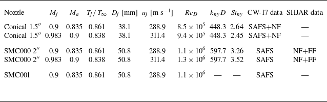


 2″
 1.5″
 Mj=0.9
 y

 Mj=0.9
 x=0.5″
 r=1.5″
 ×

 Mj=0.9
 ×


 2″
 1.5″
 Mj=0.9
 Ma=0.835
 x
 t

 Mj=0.9
 Ma=0.835
 Tj/T∞=0.861

 Mj=0.9
 Ma=0.835
 Tj/T∞=0.861
 ×

 Mj=0.983
 ×

 Mj=0.983
 ×

 2″
 Mj=0.983

 Mj=0.983
 Ma=0.9

 Mj=0.983
 Ma=0.9
 Tj/T∞=0.833

 Mj=0.983
 Ma=0.9
 Tj/T∞=0.838
 ×

 Mj=0.9
 Ma=0.835
 Tj/T∞=0.861
 Mj=0.983
 Ma=0.9
 Tj/T∞=0.838
 x−t
 ×

 (vph)
 (vg)
 Mj=0.9
 Mj=0.983
 (m,n)


 Open access

