
 Qt
 R













1. Introduction
Let us consider the stochastic differential equations (SDEs)
 \begin{align} \textrm{d} X_t & = b(X_t)\,\textrm{d} t + \sigma\,\textrm{d} L_t, \qquad X_0 = x, \end{align}
 \begin{align} \textrm{d} Y_t & = b(Y_t)\,\textrm{d} t + \sigma\,\textrm{d} B_t, \qquad Y_0 = y, \end{align}
driven by a standard d-dimensional Brownian motion
 $(B_t)_{t\geq0}$
and a stable Lévy process
 $(L_t)_{t\geq0}$
with the characteristic function
 $\mathbb{E}\,\textrm{e}^{\mathop{\textrm{i}} \xi L_t}=\textrm{e}^{-t|\xi|^\alpha/2}$
,
 $1\lt \alpha\lt 2$
; this is a standard rotationally symmetric
 $\alpha$
-stable process run at half speed. Our main assumptions are as follows:
-
(H1)
 $\sigma\in{\mathbb{R}}^{d\times d}$
is an invertible
$d \times d$
matrix.
-
(H2)
$b \in C^2({\mathbb{R}^d}, {\mathbb{R}^d})$
and there exist constants
$\theta_0\gt 0$
,
$K \ge 0$
,
$\theta_1 \ge 0$
, and
$\theta_2\geq 0$
such that, for all
$x,y,v,v_1,v_2\in {\mathbb{R}^d}$
, (1.3)
\begin{align} \langle x-y, b(x)-b(y)\rangle & \leq -\theta_0|x-y|^2+K, \end{align}
(1.4)
\begin{align} |\nabla_v b(x)| & \leq \theta_1|v|, \end{align}
(1.5)
\begin{align} |\nabla_{v_2}\nabla_{v_1} b(x)| & \leq \theta_2|v_1||v_2|. \end{align}








It is well known that under (1.4) both SDEs (1.1) and (1.2) have unique non-explosive (strong) solutions, which we denote by
 $X^x_t$
and
 $Y^y_t$
respectively. From the classical Lyapunov function criterion (see, e.g., [Reference Meyn and Tweedie9]) we know that under (H1) and (H2) the solutions to the SDEs (1.1) and (1.2) are ergodic. That means, each SDE has a unique invariant distribution (also called the ergodic measure in this case) such that, for any initial value, the distribution of the solution converges to this invariant distribution as
 $t\to\infty$
. The long-term average behaviour of the system depends only on the ensemble averages determined by this invariant distribution. For further details regarding the ergodicity of SDEs, we refer to [Reference Hairer7] (see also [Reference Sandrić, Arapostathis and Pang13] for ergodicity of Markov processes in Wasserstein distance). Denote by
 $\mu_\alpha$
and
 $\mu_2$
the respective ergodic measures of
 $X^x_t$
and
 $Y^y_t$
.
Continuing the work started in [Reference Deng, Schilling and Xu5], we establish an optimal bound between
 $X_t^x$
and
 $Y_t^y$
in total variation distance and consequently an optimal bound between
 $\mu_\alpha$
and
 $\mu_2$
. Combining this bound with a recent interpolation result from [Reference Huang, Ren and Wang8], we can extend these bounds to the Wasserstein-p distance with
 $0 < p < 1$
.
1.1. Notation
Before stating our main results, let us introduce the notation that we will use. We denote by
 $C({\mathbb{R}^d}, {\mathbb{R}}^m)$
the set of all continuous functions from
 ${\mathbb{R}^d}$
to
 ${\mathbb{R}}^m$
and by
 $C_\textrm{b}({\mathbb{R}^d}, {\mathbb{R}})$
the set of all bounded continuous functions from
 ${\mathbb{R}^d}$
to
 ${\mathbb{R}}$
. Given
 $k \in \mathbb{N}$
, denote by
 $C^k({\mathbb{R}^d}, {\mathbb{R}})$
the set of all continuous functions from
 ${\mathbb{R}^d}$
to
 ${\mathbb{R}}$
with continuous 1st-, …, kth-order derivatives, and by
 $C^k_\textrm{b}({\mathbb{R}^d}, {\mathbb{R}})$
the set of all bounded continuous functions from
 ${\mathbb{R}^d}$
to
 ${\mathbb{R}}$
with bounded continuous 1st-,…,kth-order derivatives. For a sufficiently smooth function
 $f\colon{\mathbb{R}^d}\rightarrow{\mathbb{R}}$
, the directional derivative in direction
 $v\in{\mathbb{R}^d}$
is defined as
 \begin{equation*} \nabla_{v} f(x) \,:\!= \lim_{\varepsilon\to 0} \frac{f(x+\varepsilon v)-f(x)}{\varepsilon} = \nabla f(x)\cdot v,\end{equation*}
and
 $\nabla_{v_2}\nabla_{v_1} f(x) \,:\!= \nabla_{v_2}(\nabla_{v_1} f)(x) = \nabla^2f(x){v_1}\cdot {v_2}$
for
 $v_1,v_2\in{\mathbb{R}^d}$
. The vector and matrix norms of
 $\nabla f$
and
 $\nabla^2 f$
are given by
 $|\nabla f(x)| = \sup_{v\in{\mathbb{R}^d}, |v|=1}|\nabla_v f(x)|$
and
 \begin{equation*} \|\nabla^2 f(x)\|_\textrm{op} = \sup\nolimits_{v_1,v_2\in{\mathbb{R}^d}, |v_1|=|v_2|=1}|\nabla_{v_2}\nabla_{v_1}f(x)| = \sup\nolimits_{v_1,v_2\in{\mathbb{R}^d}, |v_1|=|v_2|=1}\langle\nabla^2f(x),v_1v_2^\top\rangle_\textrm{HS}.\end{equation*}
Moreover, we define
 $\|\nabla f\|_\infty\,:\!=\sup\nolimits_{x \in {\mathbb{R}^d}} |\nabla f(x)|$
and
 $\|\nabla^2 f\|_{\textrm{op},\infty}\,:\!=\sup\nolimits_{x \in {\mathbb{R}^d}} \|\nabla^2 f(x)\|_\textrm{op}$
. This notation extends naturally to vector-valued functions
 $f=(f_{1},f_{2},\ldots,f_{d})^{\top}\colon {\mathbb{R}^d}\to {\mathbb{R}^d}$
:
 \begin{align*} \nabla f(x)v & = \nabla_{v}f(x) = (\nabla_{v}f_{1}(x),\dots,\nabla_{v}f_{d}(x))^{\top}, \\ \nabla^2f(x)v_1v_2 & = \nabla_{v_2}\nabla_{v_1}f(x) = (\nabla_{v_2}\nabla_{v_1}f_{1}(x),\dots,\nabla_{v_2}\nabla_{v_1}f_{d}(x))^{\top}.\end{align*}
For
 $x \in {\mathbb{R}^d}$
, we see
 $\nabla f(x) \in {\mathbb{R}^d}$
and
 $\nabla^2 f(x) \in {\mathbb{R}}^{d \times d}$
. The Hilbert–Schmidt inner product of two matrices
 $A, B \in {\mathbb{R}}^{d \times d}$
is
 $\langle A, B\rangle_{\textrm{HS}}=\sum_{i,j=1}^d A_{ij} B_{ij}$
, and the Hilbert–Schmidt norm is
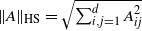 $\|A\|_{\textrm{HS}}=\sqrt{\sum_{i,j=1}^dA_{ij}^2}$
.
Recall that
 $X_t^x$
and
 $Y_t^y$
are the solutions to the SDEs (1.1) and (1.2), respectively. The operator semigroup induced by the Markov process
 $(X_t^x)_{t\geq 0}$
is
 $P_t f(x) = \mathbb{E} f(X^x_t)$
,
 $f \in C_\textrm{b}({\mathbb{R}^d},{\mathbb{R}})$
,
 $t \gt 0$
. We need to study
 $P_t$
on the Banach space
 $(C_{\textrm{lin}}({\mathbb{R}^d},{\mathbb{R}}),\|\cdot\|_\textrm{lin})$
of linearly growing continuous functions
 \begin{equation*} C_{\textrm{lin}}({\mathbb{R}^d},{\mathbb{R}}) = \bigg\{f\in C({\mathbb{R}^d},{\mathbb{R}})\colon \|f\|_\textrm{lin} \,:\!= \sup\nolimits_{x\in{\mathbb{R}^d}}\frac{|f(x)|}{1+|x|}\lt \infty\bigg\}.\end{equation*}
By [Reference Deng, Schilling and Xu5], the semigroup
 $(P_t)_{t \ge 0}$
is well defined on
 $C_{\textrm{lin}}({\mathbb{R}^d},{\mathbb{R}})$
. The infinitesimal generator
 $\mathscr{A \,}^P$
of the semigroup
 $(P_t)_{t\geq 0}$
has the domain
 \begin{align*} \mathcal{D}(\mathscr{A}^{\, P}) \,:\!= \bigg\{f\in C_{\textrm{lin}}({\mathbb{R}^d},{\mathbb{R}}) \colon g(x) &= \lim_{t\to 0}\frac{P_t f(x)-f(x)}{t} \text{ exists for all $x\in{\mathbb{R}^d}$} \\ & \quad \text{ and } g \in C_{\textrm{lin}}({\mathbb{R}^d},{\mathbb{R}})\bigg\},\end{align*}
and the infinitesimal generator
 $\mathscr{A \, }^P$
is given by
 \begin{equation*} \mathscr{A \,}^P f(x) \,:\!= \lim_{t\downarrow0}\frac{P_t f(x)-f(x)}{t}, \quad f\in \mathcal{D}(\mathscr{A \,}^P).\end{equation*}
In the same way, we can consider the semigroup
 $Q_t$
of
 $(Y_t^y)_{t\geq 0}$
and its generator
 $(\mathscr{A \,}^Q, \mathcal{D}(\mathscr{A \,}^Q))$
.
Write
 $\mathscr{C}_\textrm{b}(1) = \{h\in C_\textrm{b}({\mathbb{R}^d},{\mathbb{R}})\colon \|h\|_\infty \leq 1\}$
for the unit ball in
 $C_\textrm{b}({\mathbb{R}^d},{\mathbb{R}})$
. The total variation distance of two probability measures (on
 ${\mathbb{R}^d}$
)
 $\mu$
and
 $\nu$
is given by
 \begin{equation*} \|\mu-\nu\|_\textrm{TV} \,:\!= \sup\nolimits_{h\in\mathscr{C}_\textrm{b}(1)}|\mu(h)-\nu(h)|\end{equation*}
(as usual we write
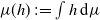 $\mu(h)\,:\!=\int h\,\textrm{d}\mu$
, etc.). It is clear that
 $\|\mu-\nu\|_\textrm{TV}\leq2$
for all probability measures
 $\mu$
and
 $\nu$
. For
 $p\in(0,1]$
, the Wasserstein-p distance (see [Reference Villani16, Theorem 1.14 and Section 7.1]) for two probability measures
 $\mu,\nu$
is given by
 \begin{equation*} \|\mu-\nu\|_{W_p}=\sup\nolimits_{|h(x)-h(y)|\leq|x-y|^p}|\mu(h)-\nu(h)|.\end{equation*}
Finally,
 $\textrm{Lip}(1)$
is the family of all Lipschitz functions
 $f\colon{\mathbb{R}^d}\to{\mathbb{R}}$
whose Lipschitz constant satisfies
 $$\|f\|_{\textrm{Lip}}\,:\!=\sup\nolimits_{x \neq y}\frac{|f(x)-f(y)|}{|x-y|} \le 1.$$
1.2. Main results
Throughout this paper, C,
 $C_1$
, and
 $C_2$
denote positive constants that may depend on
 $\theta_0$
,
 $\theta_1$
,
 $\theta_2$
, K,
 $\|\sigma\|_{\textrm{op}}$
, or
 $\|\sigma^{-1}\|_{\textrm{op}}$
, but they are always independent of d and
 $\alpha$
; their values may change from line to line. Recall that
 $\mu_\alpha$
and
 $\mu_2$
are the respective ergodic measures of
 $X^x_t$
and
 $Y^y_t$
.
Theorem 1.1. Assume (H1) and (H2). For any
 $\alpha \in (1,2)$
,
 $x,y\in{\mathbb{R}^d}$
, and
 $t \gt 0$
,
 \begin{multline*} \|\textrm{law}(X_{t}^x)-\textrm{law}(Y_{t}^y)\|_\textrm{TV} \\ \leq C_{1}\{t^{-1/2} \vee 1\}\textrm{e}^{-C_{2}t}|x-y| + \frac{Cd\log(1+d)}{\alpha-1}(2-\alpha) \cdot \{(t^{-({1}/{\alpha})+({1}/{2})}\log({1}/{t})) \vee 1\}. \end{multline*}
In particular,
 \begin{equation} \|\mu_\alpha-\mu_2\|_\textrm{TV} \leq \frac{Cd\log(1+d)}{\alpha-1}(2-\alpha). \end{equation}
We shall show that the bound in (1.6) is optimal with respect to
 $\alpha$
for a one-dimensional Ornstein–Uhlenbeck system (Proposition 5.1).
Applying a recent interpolation result established in [Reference Huang, Ren and Wang8], we obtain the following corollary.
Corollary 1.1. Assume (H1) and (H2). For any
 $p\in(0,1)$
and
 $\alpha\in(1,2)$
,
 \begin{equation*} \|\mu_\alpha-\mu_2\|_{W_p} \leq \frac{Cd^{(p+3)/2}\log(1+d)}{\alpha-1}(2-\alpha). \end{equation*}
2. A key gradient estimate for Theorem 1.1
This section is devoted to proving the following gradient estimate by integration by parts in Malliavin calculus, which is crucial for the proof of our main result.
Proposition 2.1. Assume (1.4) and (1.5). For any
 $t\in(0,1]$
,
 $\alpha\in(0,2)$
, and
 $f\in C^{2}_\textrm{b}({\mathbb{R}^d},{\mathbb{R}})$
,
 \begin{equation*} \|P_t\nabla^2f\|_{\textrm{op},\infty} \le C\sqrt{\Gamma(1+({2}/{\alpha}))}\, 2^{1/\alpha}t^{-1/\alpha}\|\nabla f\|_{\infty}. \end{equation*}
2.1. A random time-change method
This method was originally proposed by X. Zhang and our presentation follows [Reference Zhang18], with some ingredients from [Reference Chen, Deng, Schilling and Xu1]. In order to keep the presentation self-contained, we recall the basic ingredients here. Using Bochner’s subordination, it is not difficult to see that the stable Lévy process
 $(L_t)_{t\geq 0}$
with characteristic function
 $\exp\big({-}\frac 12 t |\xi|^\alpha\big)$
has the same distribution as the time-changed Brownian motion
 $(W_{S_t})_{t\geq 0}$
, where
 $(W_t)_{t\geq 0}$
is a standard Brownian motion with characteristic function
 $\exp\big({-}\frac 12 t |\xi|^2\big)$
and
 $(S_t)_{t\geq 0}$
is an independent stable subordinator (i.e. an
 ${\mathbb{R}}^+$
-valued Lévy process) with the Laplace transform
 $\mathbb{E}[\textrm{e}^{-rS_t}] = \textrm{e}^{-2^{-1}t(2r)^{\alpha/2}}$
,
 $r \gt 0$
,
 $t\geq 0$
; see, e.g., [Reference Cho, Kim, Song and Vondracek2, Reference Schilling, Song and Vondraček15, Reference Zhang18]. Since we are interested only in the distributional properties of the solution to the SDE (1.1), we may replace it by
 \begin{equation} \textrm{d}X_{t} = b(X_{t})\,\textrm{d}t + \sigma\,\textrm{d}W_{S_{t}}, \qquad X_{0}=x.\end{equation}
Let
 $\mathbb{W}$
be the space of all continuous functions from
 $[0,\infty)$
to
 ${\mathbb{R}^d}$
vanishing at
 $t=0$
; we equip
 $\mathbb{W}$
with the topology of locally uniform convergence. The corresponding Borel
 $\sigma$
-algebra is denoted by
 $\mathcal{B}(\mathbb{W})$
and
 $\mu_{\mathbb{W}}$
is the Wiener measure. Thus, the coordinate process
 $W_{t}(w)=w_{t}$
,
 $t\geq 0$
, is a standard d-dimensional Brownian motion. Let
 $\mathbb{S}$
be the space of all increasing, càdlàg (right continuous with finite left limits) functions from
 $[0,\infty)$
to
 $[0,\infty)$
vanishing at
 $t=0$
. We use on
 $\mathbb{S}$
the Skorohod metric and the corresponding Borel
 $\sigma$
-algebra
 $\mathcal{B}(\mathbb{S})$
. The probability measure
 $\mu_{\mathbb{S}}$
is chosen in such a way that, for any
 $l \in \mathbb S$
, the coordinate process
 $S_{t}(l)\,:\!=l_{t}$
is an
 $({\alpha}/{2})$
-stable subordinator. Consider the product measure space
 \begin{equation*} (\Omega,\mathcal{F},\mathbb{P}) \,:\!= (\mathbb{W}\times\mathbb{S}, \mathcal{B}(\mathbb{W})\otimes\mathcal{B}(\mathbb{S}), \mu_{\mathbb{W}}\times\mu_{\mathbb{S}}).\end{equation*}
This allows us to calculate the expectation of the solution
 $X_{t}^{x}$
to the SDE (2.1) as [Reference Zhang18]
 \begin{equation} \mathbb{E}f(X_{t}^{x}) = \int_{\mathbb{S}}\int_{\mathbb{W}}f(X_{t}^{x}(w\circ\ell))\,\mu_{\mathbb{W}}(\textrm{d}w)\, \mu_{\mathbb{S}}(\textrm{d}\ell).\end{equation}
This means that we can freeze the path of the subordinator and do all our calculations for a time-changed Brownian motion with a deterministic time change
 $\ell = (\ell_t)_{t\geq 0}\in\mathbb{S}$
. After that, we only need to make sure that our results remain stable under integration with respect to
 $\mu_{\mathbb{S}}(\textrm{d}\ell)$
. If needed, we write
 $\mathbb{E}^\mathbb{W}$
and
 $\mathbb{E}^\mathbb{S}$
for the expectation taken only in the
 $\mathbb{W}$
or
 $\mathbb{S}$
component.
For fixed
 $\ell\in\mathbb{S}$
, denote by
 $X_{t}^{\ell;x}$
the solution to the SDE
 \begin{equation} \textrm{d}X_{t}^{x;\ell} = b\big(X_{t}^{x;\ell}\big)\,\textrm{d}t + \sigma\,\textrm{d}W_{\ell_{t}-\ell_{0}}, \qquad X_{0}^{x;\ell}=x.\end{equation}
By construction,
 $W_{\ell_{t}}$
is a càdlàg
 $\mathscr{F}_{\ell_{t}}^{\mathbb{W}}$
-martingale. Thus, (H1) and (H2) guarantee that the SDE (2.3) admits a unique càdlàg
 $\mathscr{F}_{\ell_{t}}^{\mathbb{W}}$
-adapted solution
 $X_{t}^{x;\ell}$
for each initial value
 $x\in{\mathbb{R}^d}$
.
For technical reasons, we have to regularize
 $\ell\in\mathbb{S}$
. Fix
 $\varepsilon\in(0,1)$
and define
 \begin{equation*} \ell_{t}^{\varepsilon} \,:\!= \frac{1}{\varepsilon}\int_{t}^{t+\varepsilon}\ell_{s}\,\textrm{d}s + \varepsilon t = \int_{0}^{1}\ell_{\varepsilon s+t}\,\textrm{d}s + \varepsilon t.\end{equation*}
It is not hard to see that
 $\ell_t^\varepsilon\downarrow \ell_t$
(
 $t\geq 0$
) as
 $\varepsilon\downarrow 0$
, and
 $t\mapsto \ell_{t}^{\varepsilon}$
is absolutely continuous and strictly increasing. In a slight abuse of notation we write
 $X_{t}^{x;\ell^\varepsilon}$
for the solution to the SDE (2.3) with
 $\ell$
replaced by
 $\ell^\varepsilon$
.
Let
 $\gamma^{\varepsilon}$
be the inverse function of
 $\ell^{\varepsilon}$
, i.e.
 $\ell^\varepsilon\circ\gamma^{\varepsilon}_{t} = t$
for all
 $t\geq \ell_{0}^{\varepsilon}$
, and
 $\gamma^\varepsilon\circ\ell^{\varepsilon}_t=t$
for all
 $t\geq 0$
. By construction,
 $t\mapsto\gamma_{t}^{\varepsilon}$
is absolutely continuous on
 $[\ell_{0}^{\varepsilon},\infty)$
. Define
 $Z_{t}^{x;\ell^{\varepsilon}} \,:\!= X_{\gamma_{t}^{\varepsilon}}^{x;\ell^{\varepsilon}}$
,
 $t\geq \ell_{0}^{\varepsilon}$
. From (2.3) (with
 $\ell\rightsquigarrow\ell^\varepsilon$
) and with a change of variables, we see that, for
 $t\geq \ell_{0}^{\varepsilon}$
,
 \begin{equation} Z_{t}^{x;\ell^{\varepsilon}} = x + \int_{0}^{\gamma_{t}^{\varepsilon}}b\big(X_{s}^{x;\ell^{\varepsilon}}\big)\,\textrm{d}s + \sigma W_{t-\ell^\varepsilon_0} = x + \int_{\ell_{0}^{\varepsilon}}^{t}b\big(Z_{s}^{x;\ell^{\varepsilon}}\big)\dot{\gamma}_{s}^{\varepsilon}\,\textrm{d}s + \sigma W_{t-\ell^\varepsilon_0}.\end{equation}
2.2. Integration by parts via the Malliavin calculus
For fixed
 $t \gt\ell^{\varepsilon}_{0}$
, consider the Hilbert space
 $H\,:\!=L^{2}([\ell^{\varepsilon}_{0},t],{\mathbb{R}^d})$
equipped with the inner product
 $\langle f, g \rangle_{H}\,:\!= \int_{\ell^{\varepsilon}_{0}}^{t} \langle f(s),g(s) \rangle\,\textrm{d} s$
for
 $f,g\in H$
. Let
 $W=\{W(h)\colon h\in H \}$
be an isonormal Gaussian process associated with H, i.e.
 $\mathbb{E}^{\mathbb{W}}[W(f)W(g)]=\langle f, g \rangle_{H}$
,
 $f,g\in H$
, which is defined on the Wiener space
 $(\mathbb{W},\mathscr{B}(\mathbb{W}),\mu_{\mathbb{W}})$
. For the ith standard coordinate vector
 $e_{i}\in{\mathbb{R}^d}$
,
 $i=1,2,\dots,d$
, it is clear that
 $W\big(e_{1}\boldsymbol{1}_{[\ell^{\varepsilon}_{0},s]}\big), \dots, W\big(e_{d}\boldsymbol{1}_{[\ell^{\varepsilon}_{0},s]}\big)$
,
 $\ell^{\varepsilon}_{0}\le s\le t$
, are pairwise independent one-dimensional Brownian motions.
Let D denote the Malliavin derivative; the directional Malliavin derivative of a random variable
 $F\in \mathbb{D}^{1,2}$
(this is the domain of D in
 $L^{2}(\mathbb{W},\mathscr{B}(\mathbb{W}),\mu_{\mathbb{W}})$
) along
 $u\in H$
is
 \begin{equation*} D_{u}F \,:\!= \langle DF, u \rangle_{H} = \int_{\ell^{\varepsilon}_{0}}^t \langle D F(s),u(s)\rangle\,\textrm{d} s,\end{equation*}
with
 $DF \in L^2(\mathbb{W}, H)$
. For a d-dimensional random vector
 $F=(F_{1},\dots, F_{d})^{\top}$
with
 $F_{i}\in \mathbb{D}^{1,2}$
for each
 $1\leq i\leq d$
, we set
 $DF\,:\!=(DF_{1},\dots DF_{d})^{\top}$
and
 $D_{u}F= (D_{u}F_{1}, \dots, D_{u} F_{d} )^{\top}$
.
Let
 $\delta$
be the divergence operator, i.e. the adjoint of D. It is well known that, for any
 $u\in \textrm{Dom}(\delta)$
and
 $F\in \mathbb{D}^{1,2}$
,
 $\delta(u)$
satisfies
 \begin{equation} \mathbb{E}^\mathbb{W}[F\delta(u)] = \mathbb{E}^\mathbb{W}[\langle DF,u \rangle_{H}].\end{equation}
The following auxiliary lemma is crucial for proving Proposition 2.1.
Lemma 2.1. Assume (1.4) and (1.5), and fix
 $\ell\in\mathbb{S}$
and
 $\varepsilon\in(0,1)$
. For any
 $v\in{\mathbb{R}}^d$
,
 $t \gt 0$
,
 $f\in C^{1}_\textrm{b}({\mathbb{R}^d},{\mathbb{R}})$
, and
 $x\in{\mathbb{R}^d}$
,
 \begin{equation*} \big|\mathbb{E}^\mathbb{W}\big[\nabla_v f\big(X^{x;\ell^{\varepsilon}}_{t}\big)\big]\big| \leq C|v|\bigg(\frac{1}{\sqrt{\ell^{\varepsilon}_{t}-\ell^{\varepsilon}_{0}}\,} + t\bigg)\textrm{e}^{2\theta_{1}t} \sqrt{\mathbb{E}^\mathbb{W}\big[\big|f(X^{x;\ell^{\varepsilon}}_{t})\big|^{2}\big]}. \end{equation*}
Proof. By (2.4), the Malliavin derivative of
 $Z^{x;\ell^{\varepsilon}}_{t}$
along the direction
 $u\in H$
satisfies
 \begin{equation*} \textrm{d}D_{u}Z^{x;\ell^{\varepsilon}}_{t} = \big[\nabla b\big(Z^{x;\ell^{\varepsilon}}_{t}\big) \dot{\gamma}^{\varepsilon}_{t}D_{u}Z^{x;\ell^{\varepsilon}}_{t} + \sigma u(t)\big]\,\textrm{d}t, \quad t \ge \ell^{\varepsilon}_{0}. \end{equation*}
Since
 $D_{u}Z^{x;\ell^{\varepsilon}}_{\ell^{\varepsilon}_{0}}=0$
, this equation has a solution of the form
 \begin{equation} D_{u}Z^{x;\ell^{\varepsilon}}_{t} = \int_{\ell^{\varepsilon}_{0}}^{t} J_{s,t}\sigma u(s)\,\textrm{d}s, \end{equation}
where
 $J_{s,t} \,:\!= \exp\big(\int_{s}^{t}\nabla b\big(Z^{x;\ell^{\varepsilon}}_{r}\big)\dot{\gamma}^{\varepsilon}_{r}\,\textrm{d}r\big)$
,
 $\ell^{\varepsilon}_{0}\leq s\leq t$
. For any fixed
 $t \gt\ell^{\varepsilon}_{0}$
and
 $v\in{\mathbb{R}}^d$
, let
 \begin{equation} u_0(s) \,:\!= \frac{1}{t-\ell^{\varepsilon}_{0}}\,\sigma^{-1}J_{s,t}^{-1}v. \end{equation}
It can be easily verified that
 $D_{u_{0}}Z^{x;\ell^{\varepsilon}}_{t}=v$
. Combining this with the duality (2.5) between the Malliavin derivative and the divergence operator gives us, for any
 $f\in C^{1}_\textrm{b}({\mathbb{R}^d},{\mathbb{R}})$
,
 \begin{align*} \mathbb{E}^\mathbb{W}\big[\nabla_v f\big(Z^{x;\ell^{\varepsilon}}_{t}\big)\big] & = \mathbb{E}^\mathbb{W}\big[\big\langle\nabla f\big(Z^{x;\ell^{\varepsilon}}_{t}\big),v\big\rangle\big] \\ & = \mathbb{E}^\mathbb{W}\big[\big\langle\nabla f\big(Z^{x;\ell^{\varepsilon}}_{t}\big), D_{u_{0}}Z^{x;\ell^{\varepsilon}}_{t}\big\rangle\big] \\ & = \mathbb{E}^\mathbb{W}\big[D_{u_{0}}f\big(Z^{x;\ell^{\varepsilon}}_{t}\big)\big] = \mathbb{E}^\mathbb{W}\big[f\big(Z^{x;\ell^{\varepsilon}}_{t}\big)\delta(u_{0})\big]. \end{align*}
By the Cauchy–Schwarz inequality and [Reference Nualart11, Proposition 1.3.1], we obtain
 \begin{align} \big|\mathbb{E}^\mathbb{W}\big[\nabla_v f\big(Z^{x;\ell^{\varepsilon}}_{t}\big)\big]\big| & \leq \sqrt{\mathbb{E}^\mathbb{W}\big[\big|f\big(Z^{x;\ell^{\varepsilon}}_{t}\big)\big|^{2}\big]} \sqrt{\mathbb{E}^\mathbb{W}[\delta(u_{0})^{2}]} \nonumber \\ & \leq \sqrt{\mathbb{E}^\mathbb{W}\big[\big|f\big(Z^{x;\ell^{\varepsilon}}_{t}\big)\big|^{2}\big]} \sqrt{\mathbb{E}^\mathbb{W}[\|u_{0}\|_{H}^{2}+\|Du_{0}\|_{H\otimes H}^{2}]}, \end{align}
where
 $\|\cdot\|_{H\otimes H}$
denotes the norm on the tensor space
 $H\otimes H$
. By (1.4) and (2.7), we have
 \begin{align} \|u_{0}\|_{H}^{2} & = \frac{1}{(t-\ell^{\varepsilon}_{0})^{2}}\int_{\ell^{\varepsilon}_{0}}^{t} \bigg|\sigma^{-1}\exp\bigg({-}\int_{s}^{t}\nabla b\big(Z^{x;\ell^{\varepsilon}}_{r}\big) \dot{\gamma}^{\varepsilon}_{r}\,\textrm{d}r\bigg)v\bigg|^{2}\,\textrm{d}s \nonumber \\ & \le \frac{\|\sigma^{-1}\|_{\textrm{op}}^{2}|v|^2}{(t-\ell^{\varepsilon}_{0})^{2}} \int_{\ell^{\varepsilon}_{0}}^{t}\exp\bigg(2\theta_{1}\int_{s}^{t}\dot{\gamma}^{\varepsilon}_{r}\,\textrm{d}r\bigg)\, \textrm{d}s \le \frac{\|\sigma^{-1}\|_{\textrm{op}}^{2}|v|^2}{t-\ell^{\varepsilon}_{0}}\, \textrm{e}^{2\theta_{1}\gamma^{\varepsilon}_{t}}. \end{align}
Similarly, using (1.4) and (2.6) gives, for any
 $u\in H$
,
 \begin{equation} \big|D_{u}Z^{x;\ell^{\varepsilon}}_{t}\big| \leq \|\sigma\|_{\textrm{op}}\|u\|_{H} \textrm{e}^{\theta_{1}\gamma^{\varepsilon}_{t}}\sqrt{t-\ell^{\varepsilon}_{0}}. \end{equation}
Furthermore, by the chain rule for matrix exponential functions (see, e.g., [Reference Najfeld and Havel10]), we have
 \begin{align*} D_{u}J_{s,t}^{-1} & = \int_{0}^{1}\exp\bigg({-}\tau\int_{s}^{t}\nabla b\big(Z^{x;\ell^{\varepsilon}}_{r}\big) \dot{\gamma}^{\varepsilon}_{r}\,\textrm{d}r\bigg) \\ & \quad \times \bigg({-}\int_{s}^{t}\nabla^{2}b\big(Z^{x;\ell^{\varepsilon}}_{r}\big)D_{u}Z^{x;\ell^{\varepsilon}}_{r} \dot{\gamma}^{\varepsilon}_{r}\,\textrm{d}r\bigg) \exp\bigg({-}\,(1-\tau)\int_{s}^{t}\nabla b\big(Z^{x;\ell^{\varepsilon}}_{r}\big) \dot{\gamma}^{\varepsilon}_{r}\,\textrm{d}r\bigg)\,\textrm{d}\tau, \end{align*}
which, together with (1.4), (1.5), and (2.10), yields
 \begin{equation*} \|D_{u}J_{s,t}^{-1}\|_{\textrm{op},\infty} \le \|\sigma\|_{\textrm{op}}\theta_{2}\|u\|_{H} \sqrt{t-\ell^{\varepsilon}_{0}}\gamma^{\varepsilon}_{t}\textrm{e}^{2\theta_{1}\gamma^{\varepsilon}_{t}}, \quad s\in [\ell^{\varepsilon}_{0},t]. \end{equation*}
Then, it follows from (2.7) that
 \begin{align*} \|D_{u}u_{0}\|^{2}_{H} & = \frac{1}{(t-\ell^{\varepsilon}_{0})^{2}}\int_{\ell^{\varepsilon}_0}^{t} \big|\sigma^{-1}\big\{D_{u}J_{s,t}^{-1}\big\}v\big|^{2}\,\textrm{d}s \\ & \le \|\sigma^{-1}\|_{\textrm{op}}^2\|\sigma\|_{\textrm{op}}^2\theta_{2}^{2}\|u\|_{H}^{2}(\gamma^{\varepsilon}_{t})^{2} \textrm{e}^{4\theta_{1}\gamma^{\varepsilon}_{t}}|v|^2. \end{align*}
Since this holds for any
 $u\in H$
, we can deduce that
 \begin{equation*} \|Du_{0}\|^{2}_{H\otimes H} \le \|\sigma^{-1}\|_{\textrm{op}}^2\|\sigma\|_{\textrm{op}}^2 \theta_{2}^{2}(\gamma^{\varepsilon}_{t})^{2}\textrm{e}^{4\theta_{1} \gamma^{\varepsilon}_{t}}|v|^2. \end{equation*}
Combining this with (2.8) and (2.9) gives, for
 $t \gt\ell^{\varepsilon}_{0}$
,
 \begin{align*} & \big|\mathbb{E}^\mathbb{W}\big[\nabla_{v}f\big(Z^{x;\ell^{\varepsilon}}_{t}\big)\big]\big| \\ & \qquad \le \bigg(\frac{\|\sigma^{-1}\|_{\textrm{op}}|v|}{\sqrt{t-\ell^{\varepsilon}_{0}}}\, \textrm{e}^{\theta_{1}\gamma^{\varepsilon}_{t}} + \|\sigma^{-1}\|_{\textrm{op}}\|\sigma\|_{\textrm{op}} \theta_{2}\gamma^{\varepsilon}_{t}\textrm{e}^{2\theta_{1}\gamma^{\varepsilon}_{t}}|v|\bigg) \sqrt{\mathbb{E}^\mathbb{W}\big[\big|f\big(Z^{x;\ell^{\varepsilon}}_{t}\big)\big|^{2}\big]} \\ & \qquad \leq C|v|\bigg(\frac{1}{\sqrt{t-\ell^{\varepsilon}_{0}}\,} + \gamma^{\varepsilon}_{t}\bigg) \textrm{e}^{2\theta_{1}\gamma^{\varepsilon}_{t}} \sqrt{\mathbb{E}^\mathbb{W}\big[\big|f\big(Z^{x;\ell^{\varepsilon}}_{t}\big)\big|^{2}\big]}. \end{align*}
Since
 $Z_{\ell_t^\varepsilon}^{x;\ell^\varepsilon}=X_{t}^{x;\ell^\varepsilon}$
, we can replace t by
 $\ell_t^\varepsilon$
and get the desired estimate.
2.3. Proof of Proposition 2.1
Lemma 2.2. Assume (1.4) and (1.5). For any
 $\alpha\in(0,2)$
,
 $t\in(0,1]$
, and
 $f\in C^{1}_\textrm{b}({\mathbb{R}^d},{\mathbb{R}})$
,
 \begin{equation*} \|P_{t}\nabla f\|_\infty \leq C\sqrt{\Gamma(1+({2}/{\alpha}))}\,2^{1/\alpha}t^{-1/\alpha}\|f\|_\infty. \end{equation*}
Proof. Letting
 $\varepsilon\downarrow0$
in Lemma 2.1 and using
 $\ell^\varepsilon_t\downarrow\ell_t$
and [Reference Zhang18, Lemma 2.2], we get, for
 $t \gt 0$
,
 \begin{equation*} \big|\mathbb{E}^\mathbb{W}\big[\nabla_{v}f\big(X^{x;\ell}_{t}\big)\big]\big| \le C|v|(\ell_t^{-1/2}+t)\textrm{e}^{2\theta_{1}t} \sqrt{\mathbb{E}^\mathbb{W}\big[\big|f(X^{x;\ell}_{t})\big|^{2}\big]}. \end{equation*}
Now we ‘unfreeze’ the fixed path
 $\ell$
and use (2.2). From the Cauchy–Schwarz inequality we get, for all
 $t \gt 0$
,
 $v\in{\mathbb{R}}^d$
, and
 $x\in{\mathbb{R}}^d$
,
 \begin{align*} |P_t(\nabla_vf)(x)| & = \bigg|\int_{\mathbb{S}}\mathbb{E}^\mathbb{W}\big[\nabla_{v}f\big(X^{x;\ell}_{t}\big)\big]\, \mu_{\mathbb{S}}(\textrm{d}\ell)\bigg| \\ & \leq \int_{\mathbb{S}}\big|\mathbb{E}^\mathbb{W}\big[\nabla_{v}f\big(X^{x;\ell}_{t}\big)\big]\big|\, \mu_{\mathbb{S}}(\textrm{d}\ell) \\ & \leq C|v|\textrm{e}^{2\theta_{1}t}\int_{\mathbb{S}}\big(\ell_t^{-1/2}+t\big) \sqrt{\mathbb{E}^\mathbb{W}\big[\big|f(X^{x;\ell}_{t})\big|^{2}\big]}\,\mu_{\mathbb{S}}(\textrm{d}\ell) \\ & \leq C|v|\textrm{e}^{2\theta_{1}t}\sqrt{\int_{\mathbb{S}}\big(\ell_t^{-1/2}+t\big)^2\, \mu_{\mathbb{S}}(\textrm{d}\ell)}\, \sqrt{\int_{\mathbb{S}}\mathbb{E}^\mathbb{W}\big[\big|f(X^{x;\ell}_{t})\big|^{2}\big]\, \mu_{\mathbb{S}}(\textrm{d}\ell)} \\ & \leq C|v|\textrm{e}^{2\theta_{1}t}\sqrt{\int_{\mathbb{S}}(\ell_t^{-1}+t^2)\,\mu_{\mathbb{S}}(\textrm{d}\ell)}\, \sqrt{\mathbb{E}[|f(X^{x}_{t})|^{2}]} \\ & = C|v|\textrm{e}^{2\theta_{1}t}\sqrt{\mathbb{E}[S_t^{-1}]+t^2}\,\sqrt{P_t|f|^2(x)} \\ & \leq C|v|\textrm{e}^{2\theta_{1}t}\Big(\sqrt{\mathbb{E}[S_t^{-1}]}+t\Big)\|f\|_\infty. \end{align*}
From [Reference Deng and Schilling3, Lemma 4.1], we know the following moment identity for
 $\alpha\in(0,2)$
:
 \begin{equation*} \mathbb{E}[S_t^{-1}] = \frac12\,\Gamma\bigg(1+\frac{2}{\alpha}\bigg)2^{2/\alpha}t^{-2/\alpha}, \quad t \gt 0. \end{equation*}
Substituting this identity into the previous inequality, we obtain the claimed estimate for
 $t\in(0,1]$
.
Proof of Proposition
2.1. It follows from Lemma 2.2 that, for all
 $t\in(0,1]$
and
 $\alpha\in(0,2)$
,
 \begin{align*} \|P_t\nabla^2f\|_{\textrm{op},\infty} & = \sup\nolimits_{x\in{\mathbb{R}}^d}\sup\nolimits_{v_1,v_2\in{\mathbb{R}}^d,|v_1|=|v_2|=1}|P_t\nabla_{v_2}\nabla_{v_1}f(x)| \\ & \leq C\sqrt{\Gamma(1+({2}/{\alpha}))}\,2^{1/\alpha}t^{-1/\alpha} \sup\nolimits_{v_1\in{\mathbb{R}}^d,|v_1|=1}\|\nabla_{v_1}f\|_\infty. \end{align*}
Finally,
 $\sup\nolimits_{v\in{\mathbb{R}}^d,|v|=1}\|\nabla_vf\|_\infty = \sup\nolimits_{x\in{\mathbb{R}}^d}\sup\nolimits_{v\in{\mathbb{R}}^d,|v|=1} |\langle\nabla f(x),v\rangle| = \|\nabla f\|_\infty$
, and this completes the proof.
3. Gradient estimates of
${\boldsymbol{Q}}_{\boldsymbol{t}}$
and comparison of the generators

In this section we collect further tools for the proof of Theorem 1.1. Recall that
 $\mathscr{C}_\textrm{b}(1)$
is the unit ball in
 $C_\textrm{b}({\mathbb{R}^d},{\mathbb{R}})$
.
Lemma 3.1. Assume (H1) and (H2). For all
 $h\in\mathscr{C}_\textrm{b}(1)$
and
 $t \gt 0$
,
 \begin{align}\quad\ \ \ \ \|\nabla Q_{t}h\|_{\infty} & \le C_{1}\{t^{-1/2} \vee 1\}\textrm{e}^{-C_{2}t},\end{align}
 \begin{align}\|\nabla^{2}Q_{t}h\|_{\textrm{op},\infty} & \le C_{1}\{t^{-1} \vee 1\}\textrm{e}^{-C_{2}t},\end{align}
where both
 $C_1$
and
 $C_2$
do not depend on the dimension d.
Proof. By Proposition A.1 below, we have for any
 $t \gt 0$
and
 $x,y\in {\mathbb{R}^d}$
,
 \begin{equation*} \sup\nolimits_{f\in\textrm{Lip}(1)}|Q_{t}f(x)-Q_{t}f(y)| = \|\operatorname{law}(Y_t^{x})-\operatorname{law}(Y_t^{y})\|_{W_1} \le C_{1}\textrm{e}^{-C_{2}t}|x-y|. \end{equation*}
This means that, for any
 $f\in \textrm{Lip}(1)$
,
 $\| \nabla Q_{t}f \|_{\infty}\le C_{1}\textrm{e}^{-C_{2}t}$
for all
 $t \gt 0$
. On the other hand, it follows from [Reference Priola and Wang12] that, for all
 $h\in \mathscr{C}_\textrm{b}(1)$
and
 $t\in (0,1]$
,
 $\|\nabla Q_{t}h\|_{\infty}\le C t^{-1/2}$
, which implies that
 $Q_{t}h$
is a Lipschitz function with Lipschitz constant
 $C t^{-1/2}$
. Hence, if
 $t\in (0,1]$
, (3.1) holds. If
 $t \gt 1$
, we have
 \begin{equation*} \|\nabla Q_{t}h\|_{\infty} = \|\nabla Q_{t-1}\{Q_{1}h\}\|_{\infty} \le CC_1\textrm{e}^{-C_2(t-1)} = CC_1\textrm{e}^{C_2}\textrm{e}^{-C_2t}, \end{equation*}
which yields (3.1).
To prove (3.2), we first note that by [Reference Deng, Schilling and Xu5, Lemma‘2.1, (2.2)], for any
 $f\in \textrm{Lip}(1)$
and
 $t\in (0,1]$
,
 $\|\nabla^{2} Q_{t}f\|_{\textrm{op},\infty}\le C t^{-1/2}$
. From (3.1) and
 $t\in (0,2]$
, we see that for
 $h\in \mathscr{C}_\textrm{b}(1)$
the function
 $f=Q_{t/2}h$
is Lipschitz continuous with Lipschitz constant
 $C_1 (t/2)^{-1/2}\textrm{e}^{-C_2t/2}$
. Together with the previous estimate we see that
 \begin{align*} \|\nabla^{2}Q_{t}h\|_{\textrm{op},\infty} = \|\nabla^{2} Q_{t/2}\{ Q_{t/2}h\}\|_{\textrm{op},\infty} & \leq C_1(t/2)^{-1/2}\textrm{e}^{-C_2t/2}C(t/2)^{-1/2} \\ & = 2C_1Ct^{-1}\textrm{e}^{-C_2t/2}, \end{align*}
while for
 $t \gt 2$
we have, for
 $h\in \mathscr{C}_\textrm{b}(1)$
,
 \begin{equation*} \|\nabla^{2}Q_{t}h\|_{\textrm{op},\infty} = \|\nabla^{2} Q_{1}\{ Q_{t-1}h\}\|_{\textrm{op},\infty} \le C_1\textrm{e}^{-C_2(t-1)}C=C_1C\textrm{e}^{C_2}\textrm{e}^{-C_2t}. \end{equation*}
This completes the proof of (3.2).
In the following lemma, we will frequently need the constants
 \begin{equation*} A(d,\alpha) \,:\!= \frac{\alpha\Gamma(({d+\alpha})/{2})}{2^{2-\alpha}\pi^{d/2}\Gamma(1-(\alpha/2))}, \qquad \omega_{d-1} \,:\!= \frac{2\pi^{d/2}}{\Gamma({d}/{2})},\end{equation*}
which can be estimated as follows (see [Reference Deng, Schilling and Xu5, Lemma 3.3]):
 \begin{equation} \frac{A(d,\alpha)\omega_{d-1}}{d(2-\alpha)}\leq C \quad\text{and}\quad \bigg| \frac{A(d,\alpha)\omega_{d-1}}{d(2-\alpha)} - 1\bigg| \leq C(2-\alpha)\log(1+d).\end{equation}
Lemma 3.2. Assume (H1) and (H2).
-
1. For any
$\alpha \in (1,2)$
and
$0 \lt s \lt t\le 1$
,
\begin{multline*} \sup\nolimits_{h\in\mathscr{C}_b(1)}\big\|P_{t-s}\big(\mathscr{A \,}^P-\mathscr{A \,}^Q\big)Q_{s}h\big\|_{\infty} \\ \leq C(t-s)^{-1/\alpha}s^{-1/2}\bigg(3-\alpha-\frac{1}{3-\alpha}s^{1-({\alpha}/{2})}\bigg)d\log(1+d) + \frac{C}{\alpha-1}(2-\alpha)s^{-1/2}d. \end{multline*}
-
2. For any
$\alpha \in (1,2)$
,
$0 \lt s \lt t\le 1$
, and
$k=1,2,\dots$
,
\begin{multline*} \sup\nolimits_{h\in\mathscr{C}_b(1)}\big\|P_{t-s}\big(\mathscr{A \,}^P-\mathscr{A \,}^Q\big)Q_{s+k}h\big\|_{\infty} \\ \leq C_1(2-\alpha)\bigg((t-s)^{-1/\alpha}+\frac{1}{\alpha-1}\bigg)\textrm{e}^{-C_2k}d\log(1+d). \end{multline*}


Proof. We begin with some general preparations. Let
 $h\in\mathscr{C}_\textrm{b}(1)$
and set
 $f\,:\!=Q_{s+k}h$
for
 $k\in\{0,1,2,\dots\}$
. It is not hard to see that, for any
 $f\in C^2_\textrm{b}({\mathbb{R}^d},{\mathbb{R}})$
, the generators of the semigroups
 $(P_t)_{t\geq 0}$
and
 $(Q_t)_{t\geq 0}$
are given by
 \begin{align*} \mathscr{A \,}^Pf(x) & = \langle\nabla f(x),b(x)\rangle + \int\limits_{{{\mathbb{R}^d}\setminus\{0\}}}\big[f(x+\sigma z) - f(x) - \langle\nabla f(x),\sigma z\rangle\boldsymbol{1}_{(0,1)}(|z|)\big] \frac{A(d,\alpha)}{|z|^{d+\alpha}}\,\textrm{d}z, \\ \mathscr{A \,}^Qf(x) & = \langle\nabla f(x),b(x)\rangle + \frac12\langle\nabla^2f(x),\sigma\sigma^{\top}\rangle_{\textrm{HS}}. \end{align*}
Therefore,
 \begin{align*} & \big(\mathscr{A \,}^P-\mathscr{A \,}^Q\big)f(x) \\ & \qquad = \bigg\{\int_{|z|<1}[f(x+\sigma z)-f(x)-\langle\nabla f(x),\sigma z\rangle] \frac{A(d,\alpha)}{|z|^{d+\alpha}}\,\textrm{d}z - \frac12\langle\nabla^2f(x),\sigma\sigma^{\top}\rangle_{\textrm{HS}}\bigg\} \\ & \qquad\quad + \int_{|z|\geq 1}[f(x+\sigma z)-f(x)]\frac{A(d,\alpha)}{|z|^{d+\alpha}}\,\textrm{d}z \, =\!: \, \mathsf{J}_1(x) + \mathsf{J}_2(x). \end{align*}
By the first inequality in (3.3), for all
 $\alpha \in (1,2)$
,
 \begin{align} |\mathsf{J}_2(x)| & \leq \int_{|z|\geq 1}|f(x+\sigma z)-f(x)|\frac{A(d,\alpha)}{|z|^{d+\alpha}}\,\textrm{d}z \nonumber \\ & \leq \|\nabla f\|_{\infty}\|\sigma\|_{\textrm{op}}\int_{|z|\geq 1}|z| \frac{A(d,\alpha)}{|z|^{d+\alpha}}\,\textrm{d}z \nonumber \\ & = \|\nabla f\|_{\infty}\|\sigma\|_{\textrm{op}}\frac{A(d,\alpha)\omega_{d-1}}{\alpha-1} \leq \frac{C}{\alpha-1}\|\nabla f\|_{\infty}(2-\alpha) d. \end{align}
We can rewrite
 $\mathsf{J}_1(x)$
in the following form:
 \begin{align*} \mathsf{J}_1(x) & = \int_{|z| < 1}[f(x+\sigma z)-f(x)-\langle\nabla f(x),\sigma z\rangle] \frac{A(d,\alpha)}{|z|^{d+\alpha}}\,\textrm{d}z - \frac12\langle\nabla^2f(x),\sigma\sigma^{\top}\rangle_{\textrm{HS}} \\ & = \int_{|z| < 1}\int_0^1\langle\nabla^2f(x+r\sigma z),(\sigma z)(\sigma z)^{\top}\rangle_{\textrm{HS}} (1-r)\,\textrm{d}r\frac{A(d,\alpha)}{|z|^{d+\alpha}}\,\textrm{d}z - \frac12\langle\nabla^2f(x),\sigma\sigma^{\top}\rangle_{\textrm{HS}} \\ & = \bigg\{\int_{|z| < 1}\int_0^1\langle\nabla^2f(x),(\sigma z)(\sigma z)^{\top}\rangle_{\textrm{HS}} (1-r)\,\textrm{d}r\frac{A(d,\alpha)}{|z|^{d+\alpha}}\,\textrm{d}z - \frac12\langle\nabla^2f(x),\sigma\sigma^{\top}\rangle_{\textrm{HS}}\bigg\} \\ & \quad + \int_{|z| < 1}\int_0^1\langle\nabla^2f(x+r\sigma z) - \nabla^2f(x), (\sigma z)(\sigma z)^{\top}\rangle_{\textrm{HS}}(1-r)\,\textrm{d}r \frac{A(d,\alpha)}{|z|^{d+\alpha}}\,\textrm{d}z \\ & \, =\!: \, \mathsf{J}_{11}(x) + \mathsf{J}_{12}(x). \end{align*}
Using the symmetry of the measure
 $\rho(\textrm{d}z) = |z|^{-d-\alpha}\,\textrm{d}z$
, it is clear that
 $\int_{|z|\leq 1}z_i z_j\,\rho(\textrm{d}z) = \delta_{ij}(1/d)\int_{|z|\leq 1}|z|^2\,\rho(\textrm{d}z)$
, and so we get
 \begin{align*} & \int_{|z| < 1}\int_0^1\langle\nabla^2f(x),(\sigma z)(\sigma z)^{\top}\rangle_{\textrm{HS}}(1-r)\textrm{d}r \frac{A(d,\alpha)}{|z|^{d+\alpha}}\,\textrm{d}z \\ & \qquad = \frac12\int_{|z| < 1}\langle\nabla^2f(x),\sigma(zz^{\top})\sigma^{\top}\rangle_{\textrm{HS}} \frac{A(d,\alpha)}{|z|^{d+\alpha}}\,\textrm{d}z \\ & \qquad = \frac12\frac{1}{d}\int_{|z| < 1}\langle\nabla^2f(x),|z|^2\sigma\sigma^{\top}\rangle_{\textrm{HS}} \frac{A(d,\alpha)}{|z|^{d+\alpha}}\,\textrm{d}z \\ & \qquad = \frac{1}{2d}\langle\nabla^2f(x),\sigma\sigma^{\top}\rangle_{\textrm{HS}} \int_{|z|<1}\frac{A(d,\alpha)}{|z|^{d+\alpha-2}}\,\textrm{d}z = \frac{A(d,\alpha)\omega_{d-1}}{2d(2-\alpha)}\langle\nabla^2f(x),\sigma\sigma^{\top}\rangle_{\textrm{HS}}. \end{align*}
Combining this with (3.3), Proposition 2.1, and the fact that
 $\|\sigma\sigma^\top\|_\textrm{HS}\leq\sqrt{d}\|\sigma\sigma^\top\|_\textrm{op}\leq\sqrt{d}\|\sigma\|_\textrm{op}^2$
, we obtain, for all
 $\alpha \in (1,2)$
,
 \begin{align} |P_{t-s}\mathsf{J}_{11}(x)| & = \bigg|\frac12\bigg[\frac{A(d,\alpha)\omega_{d-1}}{d(2-\alpha)}-1\bigg] \langle P_{t-s}\nabla^2f(x),\sigma\sigma^{\top}\rangle_{\textrm{HS}}\bigg| \nonumber \\ & \leq \frac12\bigg|\frac{A(d,\alpha)\omega_{d-1}}{d(2-\alpha)}-1\bigg| \|P_{t-s}\nabla^{2}f(x)\|_{\textrm{HS}}\|\sigma\sigma^\top\|_{\textrm{HS}} \nonumber \\ & \leq \frac12\bigg|\frac{A(d,\alpha)\omega_{d-1}}{d(2-\alpha)}-1\bigg| d\|P_{t-s}\nabla^{2}f(x)\|_{\textrm{op},\infty}\|\sigma\|_\textrm{op}^2 \nonumber \\ & \leq C(2-\alpha)(t-s)^{-1/\alpha}\|\nabla f\|_\infty d\log(1+d). \end{align}
Let us now estimate
 $P_{t-s}\mathsf{J}_{12}(x)$
. It follows from Proposition 2.1 that, for any
 $r\in[0,1]$
and
 $\alpha \in (1,2)$
,
 \begin{align*} & \big|\langle P_{t-s}[\nabla^2(f(x+r\sigma z)-f(x))], (\sigma z)(\sigma z)^{\top}\rangle_{\textrm{HS}}\big| \\ & \qquad \le \|P_{t-s}\nabla^2\{f(\cdot+r\sigma z)-f(\! \cdot \!)\}(x)\|_{\textrm{op}}|\sigma z|^2 \\ & \qquad \le C(t-s)^{-1/\alpha}\|\nabla\{f(\cdot+r\sigma z)-f(\! \cdot \!)\}\|_\infty|\sigma z|^2 \\ & \qquad \le C(t-s)^{-1/\alpha}\{[2\|\nabla f\|_\infty]\wedge[\|\nabla^2 f\|_{\textrm{op},\infty}r|\sigma z|]\} |\sigma z|^2 \\ & \qquad \le C(t-s)^{-1/\alpha}\{\|\nabla f\|_\infty\wedge[\|\nabla^2 f\|_{\textrm{op},\infty}|z|]\}|z|^2. \end{align*}
This yields, for
 $\alpha \in (1,2)$
,
 \begin{align} & |P_{t-s}\mathsf{J}_{12}(x)| \nonumber \\ & \quad \leq \int_{|z|<1}\int_0^1|\langle P_{t-s}\nabla^2f(x+r\sigma z)-P_{t-s}\nabla^2f(x), (\sigma z)(\sigma z)^{\top}\rangle_{\textrm{HS}}|(1-r)\,\textrm{d}r \frac{A(d,\alpha)}{|z|^{d+\alpha}}\,\textrm{d}z \nonumber \\ & \quad \leq C(t-s)^{-1/\alpha}\int_{|z|<1}\bigg(\int_0^1(1-r)\,\textrm{d}r\bigg) \{\|\nabla f\|_\infty\wedge[\|\nabla^2 f\|_{\textrm{op},\infty}|z|]\}|z|^{2} \frac{A(d,\alpha)}{|z|^{d+\alpha}}\,\textrm{d}z \nonumber \\ & \quad = \frac{C}{2}(t-s)^{-1/\alpha}\int_{|z|<1}\{\|\nabla f\|_\infty\wedge[\|\nabla^2 f\|_{\textrm{op},\infty}|z|]\} \frac{A(d,\alpha)}{|z|^{d+\alpha-2}}\,\textrm{d}z. \end{align}
Now we are ready to prove Lemma 3.2.
-
(i) Take, in the above calculations,
$k=0$
. Note that
$f=Q_{s}h$
and
$s\in(0,1)$
. By (3.1), we get
$\|\nabla f\|_\infty\leq Cs^{-1/2}$
. Then, by (3.4) and (3.5), for all
$\alpha\in (1,2)$
, Moreover, by (3.2),
\begin{align*} |\mathsf{J}_{2}(x)| & \leq \frac{C}{\alpha-1}(2-\alpha)s^{-1/2}d, \\ |P_{t-s}\mathsf{J}_{11}(x)| & \leq C(2-\alpha)(t-s)^{-1/\alpha}s^{-1/2} d\log(1+d), \end{align*}
$\|\nabla^2 f\|_{\textrm{op},\infty}\leq Cs^{-1}$
. It follows from the first inequality in (3.3) that, for all
$\alpha\in(0,2)$
, Therefore, we obtain from (3.6) that, for
\begin{equation*} \frac{A(d,\alpha)\omega_{d-1}}{2-\alpha}\leq C d. \end{equation*}
$\alpha \in (1,2)$
, Combining these estimates we get, for all
\begin{align*} |P_{t-s}\mathsf{J}_{12}(x)| & \leq C(t-s)^{-1/\alpha}\int_{|z|<1}\{s^{-1/2}\wedge [s^{-1}|z|]\} \frac{A(d,\alpha)}{|z|^{d+\alpha-2}}\,\textrm{d}z \\ & = C(t-s)^{-1/\alpha}\bigg(\int_{|z|\leq\sqrt{s}}s^{-1}|z|\frac{A(d,\alpha)}{|z|^{d+\alpha-2}}\,\textrm{d}z + \int_{\sqrt{s}<|z|<1}s^{-1/2}\frac{A(d,\alpha)}{|z|^{d+\alpha-2}}\,\textrm{d}z\bigg) \\ & = C(t-s)^{-1/\alpha}s^{-1/2}A(d,\alpha)\omega_{d-1} \bigg(s^{-1/2}\int_0^{\sqrt{s}}r^{2-\alpha}\,\textrm{d}r + \int_{\sqrt{s}}^1r^{1-\alpha}\,\textrm{d}r\bigg) \\ & = C(t-s)^{-1/\alpha}s^{-1/2}\bigg(1-\frac{1}{3-\alpha}s^{1-({\alpha}/{2})}\bigg) \frac{A(d,\alpha)\omega_{d-1}}{2-\alpha} \\ & \leq C(t-s)^{-1/\alpha}s^{-1/2}\bigg(1-\frac{1}{3-\alpha}s^{1-({\alpha}/{2})}\bigg)d. \end{align*}
$\alpha\in (1,2)$
,
$x\in{\mathbb{R}^d}$
, and
$0 \lt s \lt t\leq1$
, from which we immediately get the first part of the lemma.
\begin{align*} & \big|P_{t-s}\big(\mathscr{A \,}^P-\mathscr{A \,}^Q\big)f(x)\big| \\ & \quad \leq |P_{t-s}\mathsf{J}_{11}(x)| + |P_{t-s}\mathsf{J}_{12}(x)| + |P_{t-s}\mathsf{J}_{2}(x)| \\ & \quad \leq C(t-s)^{-1/\alpha}s^{-1/2}\bigg[(2-\alpha)+\bigg(1-\frac{1}{3-\alpha}s^{1-({\alpha}/{2})}\bigg)\bigg] d\log(1+d)\\ &\qquad + \frac{C}{\alpha-1}(2-\alpha)s^{-1/2}d, \end{align*}
-
(ii) Let
$k\geq1$
. Since
$f=Q_{s+k}h$
and
$s+k\gt 1$
, it follows from Lemma 3.1 that
$\|\nabla f\|_\infty\leq C_1\textrm{e}^{-C_2k}$
and
$\|\nabla^2 f\|_{\textrm{op},\infty}\leq C_1\textrm{e}^{-C_2k}$
. Using (3.4) and (3.5) implies that, for all
$\alpha\in(1,2)$
, With the first estimate in (3.3), it is easy to check that, for any
\begin{align*} |\mathsf{J}_{2}(x)| & \leq \frac{C_1}{\alpha-1}(2-\alpha)\textrm{e}^{-C_2k}d, \\ |P_{t-s}\mathsf{J}_{11}(x)| & \leq C_1(2-\alpha)(t-s)^{-1/\alpha}\textrm{e}^{-C_2k} d\log(1+d). \end{align*}
$\alpha \in (0,2)$
, the following estimate holds:Using (3.6) we get, for all
\begin{equation*} \frac{A(d,\alpha)\omega_{d-1}}{3-\alpha}\leq C(2-\alpha)d. \end{equation*}
$\alpha\in(1,2)$
, Finally, combining all the estimates, we conclude that, for all
\begin{align*} |P_{t-s}\mathsf{J}_{12}(x)| & \leq C_1(t-s)^{-1/\alpha}\int_{|z|\leq1}\textrm{e}^{-C_2k}|z|\frac{A(d,\alpha)}{|z|^{d+\alpha-2}}\,\textrm{d}z \\ & = C_1(t-s)^{-1/\alpha}\textrm{e}^{-C_2k}A(d,\alpha)\omega_{d-1}\int_0^1r^{2-\alpha}\,\textrm{d}r \\ & = C_1(t-s)^{-1/\alpha}\textrm{e}^{-C_2k}\frac{A(d,\alpha)\omega_{d-1}}{3-\alpha} \leq C_1(2-\alpha)(t-s)^{-1/\alpha}\textrm{e}^{-C_2k}d. \end{align*}
$\alpha\in (1,2)$
, which completes the proof of the second part of the lemma.
\begin{align*} \big|P_{t-s}\big(\mathscr{A \,}^P-\mathscr{A \,}^Q\big)f(x)\big| & \leq |P_{t-s}\mathsf{J}_{11}(x)| + |P_{t-s}\mathsf{J}_{12}(x)| + |P_{t-s}\mathsf{J}_{2}(x)| \\ & \leq C_1(2-\alpha)(t-s)^{-1/\alpha}\textrm{e}^{-C_2k}d\log(1+d) + \frac{C_1}{\alpha-1}(2-\alpha)\textrm{e}^{-C_2k}d, \end{align*}












4. Proofs of Theorem 1.1 and Corollary 1.1
Lemma 4.1. For any
 $t\in(0,1]$
and
 $\alpha\in (1,2)$
,
 \begin{equation*} \int_{0}^{t}(t-s)^{-{1}/{\alpha}}s^{-1/2} \bigg(3-\alpha-\frac{1}{3-\alpha}s^{1-({\alpha}/{2})}\bigg)\,\textrm{d}s \le \frac{C}{\alpha-1}(2-\alpha)t^{-({1}/{\alpha})+({1}/{2})}\bigg(1+\log\frac{1}{t}\bigg). \end{equation*}
Proof. Using the elementary estimate
 \begin{equation*} 1-s^\kappa = -\log s\int_0^\kappa s^x\,\textrm{d}x \leq (\! -\log s)\kappa = \kappa\log\frac1s, \quad 0 \lt s \lt 1,\ \kappa\gt 0, \end{equation*}
yields, for all
 $s\in (0,1)$
and
 $\alpha\in(0,2)$
,
 \begin{align*} 3-\alpha-\frac{s^{1-({\alpha}/{2})}}{3-\alpha} & = \frac{(4-\alpha)(2-\alpha)}{3-\alpha}+\frac{1}{3-\alpha}(1-s^{1-({\alpha}/{2})}) \\ & < 2(2-\alpha)+\bigg(1-\frac\alpha2\bigg)\log\frac{1}{s} \\ & < 2(2-\alpha)\bigg(1+\log\frac{1}{s}\bigg). \end{align*}
This, together with the change of variables
 $s=t\tau$
, implies that, for any
 $t\in (0,1]$
and
 $\alpha\in(1,2)$
,
 \begin{align} & \int_{0}^{t}(t-s)^{-{1}/{\alpha}}s^{-1/2} \bigg(3-\alpha-\frac{1}{3-\alpha}s^{1-({\alpha}/{2})}\bigg)\,\textrm{d}s \nonumber \\ &\qquad \leq 2(2-\alpha)\int_{0}^{t}(t-s)^{-{1}/{\alpha}}s^{-1/2}\bigg(1+\log\frac{1}{s}\bigg)\,\textrm{d}s \nonumber \\ &\qquad = 2(2-\alpha)t^{-({1}/{\alpha})+({1}/{2})}\int_{0}^{1}(1-\tau)^{-{1}/{\alpha}}\tau^{-{1}/{2}} \bigg(1+\log\frac{1}{t\tau}\bigg)\,\textrm{d}\tau \nonumber \\ &\qquad = 2(2-\alpha)t^{-({1}/{\alpha})+({1}/{2})} \bigg(\int_{0}^{1}(1-\tau)^{-{1}/{\alpha}}\tau^{-{1}/{2}}\bigg(1+\log\frac{1}{\tau}\bigg)\,\textrm{d}\tau + \operatorname{B}\bigg(1-\frac{1}{\alpha},\frac{1}{2}\bigg)\log\frac1t\bigg). \end{align}
As usual,
 $\operatorname{B}(\cdot,\cdot)$
is Euler’s Beta function. From
 $\Gamma(x)<1/x$
for
 $x\in(0,1)$
, we see that, for all
 $\alpha\in(1,2)$
,
 \begin{equation} \operatorname{B}\bigg(1-\frac{1}{\alpha},\frac{1}{2}\bigg) = \frac{\Gamma(1-({1}/{\alpha}))\Gamma({1}/{2})}{\Gamma((3/2)-({1}/{\alpha}))} < \sqrt{\pi}\,\Gamma(1-({1}/{\alpha})) < \sqrt{\pi}\,\frac{\alpha}{\alpha-1} < \frac{2\sqrt{\pi}}{\alpha-1}. \end{equation}
Noting that there exists some constant
 $C\gt 0$
such that
 $1+\log\tfrac{1}{\tau}\leq C\tau^{-1/4}$
for all
 $\tau\in(0,1)$
, as in (4.2) we have, for all
 $\alpha\in(1,2)$
,
 \begin{align*} & \int_{0}^{1}(1-\tau)^{-{1}/{\alpha}}\tau^{-{1}/{2}}\bigg(1+\log\frac{1}{\tau}\bigg)\,\textrm{d}\tau \\ &\qquad \leq C\int_{0}^{1}(1-\tau)^{-{1}/{\alpha}}\tau^{-{3}/{4}}\,\textrm{d}\tau \\ &\qquad = C\operatorname{B}\bigg(1-\frac{1}{\alpha},\frac{1}{4}\bigg) \\ &\qquad = C\frac{\Gamma(1-({1}/{\alpha}))\Gamma({1}/{4})}{\Gamma((5/4)-({1}/{\alpha}))} < C\frac{\Gamma({1}/{4})}{\Gamma({3}/{4})}\Gamma\bigg(1-\frac{1}{\alpha}\bigg) < \frac{\Gamma({1}/{4})}{\Gamma({3}/{4})}\frac{2C}{\alpha-1}. \end{align*}
Proposition 4.1. Assume (H1) and (H2). For all
 $\alpha \in (1,2)$
and
 $t \gt 0$
,
 \begin{equation*} \sup\nolimits_{x\in{\mathbb{R}}^d}\|\textrm{law}(X_t^x)-\textrm{law}(Y_t^x)\|_\textrm{TV} \leq \frac{Cd^{3/2}}{\alpha-1}(2-\alpha)\cdot\bigg\{\bigg(t^{-({1}/{\alpha})+({1}/{2})}\log\frac{1}{t}\bigg)\vee1\bigg\}. \end{equation*}
Proof. Recall that
 $\mathscr{C}_\textrm{b}(1)$
is the unit ball in
 $C_\textrm{b}({\mathbb{R}^d},{\mathbb{R}})$
. Since
 \begin{align*} & \qquad\qquad\qquad\qquad \|\textrm{law}(X_t^x)-\textrm{law}(Y_t^x)\|_\textrm{TV}=\sup\nolimits_{h\in \mathscr{C}_{b}(1)}|P_t h(x)-Q_t h(x)| \\ & \textrm{and} \\ &\qquad\qquad\qquad P_t h-Q_t h = -\int_0^t\frac{\textrm{d}}{\textrm{d}s}\,P_{t-s} Q_s h \,\textrm{d}s = \int_0^t P_{t-s}\big(\mathscr{A \,}^P-\mathscr{A \,}^Q\big)Q_s h\,\textrm{d}s, \\ & \textrm{we get} \\ & \qquad \sup\nolimits_{x\in{\mathbb{R}}^d}\|\textrm{law}(X_t^x)-\textrm{law}(Y_t^x)\|_\textrm{TV} = \sup\nolimits_{h\in\mathscr{C}_\textrm{b}(1)}\sup\nolimits_{x\in{\mathbb{R}}^d} \bigg|\int_0^t P_{t-s}\big(\mathscr{A \,}^P-\mathscr{A \,}^Q\big)Q_s h(x)\,\textrm{d}s\bigg|. \end{align*}
From Lemmas 3.2 and 4.1 we see that, for all
 $\alpha\in(1,2)$
and
 $t\in(0,1]$
,
 \begin{align} & \sup\nolimits_{h\in\mathscr{C}_\textrm{b}(1)}\int_0^t\big\|P_{t-s}\big(\mathscr{A \,}^P-\mathscr{A \,}^Q\big)Q_s h\big\|_\infty\, \textrm{d}s \nonumber \\ & \qquad \leq Cd\log(1+d)\cdot\int_{0}^{t}(t-s)^{-{1}/{\alpha}}s^{-1/2} \bigg(3-\alpha-\frac{1}{3-\alpha}s^{1-({\alpha}/{2})}\bigg)\,\textrm{d}s \nonumber \\ & \qquad\quad + \frac{Cd}{\alpha-1}(2-\alpha)\int_0^ts^{-1/2}\,\textrm{d}s \nonumber \\ & \qquad \leq \frac{Cd\log(1+d)}{\alpha-1}(2-\alpha)t^{-({1}/{\alpha})+({1}/{2})}\bigg(1+\log\frac{1}{t}\bigg) + \frac{2Cd}{\alpha-1}(2-\alpha)t^{1/2} \nonumber \\ & \qquad \leq \frac{C_1d\log(1+d)}{\alpha-1}(2-\alpha)t^{-({1}/{\alpha})+({1}/{2})}\bigg(1+\log\frac{1}{t}\bigg). \end{align}
Combining this with
 \begin{equation*} \sup\nolimits_{x\in{\mathbb{R}}^d}\|\textrm{law}(X_t^x)-\textrm{law}(Y_t^x)\|_\textrm{TV} \leq \sup\nolimits_{h\in\mathscr{C}_\textrm{b}(1)}\int_0^t\big\|P_{t-s}\big(\mathscr{A \,}^P-\mathscr{A \,}^Q\big)Q_sh\big\|_\infty\, \textrm{d}s \end{equation*}
proves the assertion for
 $t\in(0,1]$
.
Next, we consider the case
 $t \gt 1$
. Denote by
 $\lfloor t\rfloor$
the largest integer less than or equal to
 $t \gt 1$
. From
 \begin{align*} & \int_0^t P_{t-s}\big(\mathscr{A \,}^P-\mathscr{A \,}^Q\big)Q_s h\,\textrm{d}s \\ &\qquad = \sum_{k=0}^{\lfloor t\rfloor-1}\int_{k}^{k+1}P_{t-k-1}P_{k+1-s} \big(\mathscr{A \,}^P-\mathscr{A \,}^Q\big)Q_sh\,\textrm{d}s + \int_{\lfloor t\rfloor}^tP_{t-s}\big(\mathscr{A \,}^P-\mathscr{A \,}^Q\big)Q_s h\,\textrm{d}s \\ & \qquad= \sum_{k=0}^{\lfloor t\rfloor-1}\int_{0}^{1}P_{t-k-1}P_{1-s} \big(\mathscr{A \,}^P-\mathscr{A \,}^Q\big)Q_{s+k} h\,\textrm{d}s + \int_{0}^{t-\lfloor t\rfloor}P_{t-\lfloor t\rfloor-s}\big(\mathscr{A \,}^P-\mathscr{A \,}^Q\big)Q_{\lfloor t\rfloor +s}h\, \textrm{d}s, \end{align*}
we obtain
 \begin{align} \sup\nolimits_{x\in{\mathbb{R}}^d}\|\textrm{law}(X_t^x)-\textrm{law}(Y_t^x)\|_\textrm{TV} & \leq \sup\nolimits_{h\in\mathscr{C}_\textrm{b}(1)}\int_{0}^{1}\big\|P_{1-s} \big(\mathscr{A \,}^P-\mathscr{A \,}^Q\big)Q_{s}h\big\|_\infty\,\textrm{d}s \nonumber \\ & \quad + \sum_{k=1}^{\lfloor t\rfloor-1}\sup\nolimits_{h\in\mathscr{C}_\textrm{b}(1)}\int_{0}^{1} \big\|P_{1-s}\big(\mathscr{A \,}^P-\mathscr{A \,}^Q\big)Q_{s+k}h\big\|_\infty\,\textrm{d}s \nonumber \\ & \quad + \sup\nolimits_{h\in\mathscr{C}_\textrm{b}(1)}\int_{0}^{t-\lfloor t\rfloor} \big\|P_{t-\lfloor t\rfloor-s}\big(\mathscr{A \,}^P-\mathscr{A \,}^Q\big)Q_{\lfloor t\rfloor +s}h\big\|_\infty\, \textrm{d}s, \end{align}
where we use the ‘empty-sum convention’
 $\sum_{k=1}^0\dots=0$
. Using (4.3) with
 $t=1$
, we see that, for all
 $\alpha\in(1,2)$
,
 \begin{equation*} \sup\nolimits_{h\in\mathscr{C}_\textrm{b}(1)}\int_0^1\big\|P_{1-s}\big(\mathscr{A \,}^P-\mathscr{A \,}^Q\big)Q_sh\big\|_{\infty}\, \textrm{d}s \leq \frac{Cd\log(1+d)}{\alpha-1}(2-\alpha). \end{equation*}
By Lemma 3.2(ii), we find that, for all
 $\alpha \in (1,2)$
,
 \begin{align*} & \sup\nolimits_{h\in\mathscr{C}_\textrm{b}(1)}\int_{0}^{1}\big\|P_{1-s}\big(\mathscr{A \,}^P-\mathscr{A \,}^Q\big)Q_{s+k}h\big\|_\infty \,\textrm{d}s \\ & \qquad \leq C_1(2-\alpha)\textrm{e}^{-C_2k}\int_0^1\bigg((1-s)^{-1/\alpha}+\frac{1}{\alpha-1}\bigg)\, \textrm{d}s \cdot d\log(1+d) \\ & \qquad = C_1(2-\alpha)\textrm{e}^{-C_2k}\bigg(\frac{\alpha}{\alpha-1}+\frac{1}{\alpha-1}\bigg)d\log(1+d) \\ & \qquad \leq \frac{3C_1d\log(1+d)}{\alpha-1}(2-\alpha)\textrm{e}^{-C_2k} \end{align*}
and
 \begin{align*} & \sup\nolimits_{h\in\mathscr{C}_\textrm{b}(1)}\int_{0}^{t-\lfloor t\rfloor} \big\|P_{t-\lfloor t\rfloor-s}\big(\mathscr{A \,}^P-\mathscr{A \,}^Q\big)Q_{s+\lfloor t\rfloor}h\big\|_\infty\,\textrm{d}s \\ & \qquad \leq C_1(2-\alpha)\textrm{e}^{-C_2\lfloor t\rfloor}\int_{0}^{t-\lfloor t\rfloor} \bigg((t-\lfloor t\rfloor-s)^{-1/\alpha}+\frac{1}{\alpha-1}\bigg)\,\textrm{d}s \cdot d\log(1+d) \\ & \qquad = C_1(2-\alpha)\textrm{e}^{-C_2\lfloor t\rfloor} \bigg((t-\lfloor t\rfloor)^{1-1/\alpha}\frac{\alpha}{\alpha-1} + \frac{1}{\alpha-1}(t-\lfloor t\rfloor)\bigg)d\log(1+d) \\ & \qquad \leq C_1(2-\alpha)\bigg(\frac{\alpha}{\alpha-1}+\frac{1}{\alpha-1}\bigg)d\log(1+d) \\ & \qquad \leq \frac{3C_1d\log(1+d)}{\alpha-1}(2-\alpha). \end{align*}
Substituting these estimates into (4.4) shows that, for all
 $t\geq1$
and
 $\alpha\in(1,2)$
,
 \begin{align*} \sup\nolimits_{x\in{\mathbb{R}}^d}\|\textrm{law}(X_t^x)-\textrm{law}(Y_t^x)\|_\textrm{TV} & \leq \frac{C_1d\log(1+d)}{\alpha-1}(2-\alpha) \Bigg(1+\sum_{k=1}^{\lfloor t\rfloor-1}\textrm{e}^{-C_2k}\Bigg) \\ & \leq \frac{Cd\log(1+d)}{\alpha-1}(2-\alpha). \end{align*}
This completes the proof.
Proposition 4.2. Assume (H1) and (H2). For all
 $x,y\in {\mathbb{R}^d}$
and
 $t \gt 0$
,
 \begin{equation*} \|\textrm{law}(Y^{x}_{t})-\textrm{law}(Y^{y}_{t})\|_{\textrm{TV}} \leq C_{1}\{t^{-1/2} \vee 1\}\textrm{e}^{-C_{2}t}|x-y|. \end{equation*}
Proof. By the definition of the total variation norm
 $\|\cdot\|_\textrm{TV}$
, we have
 \begin{equation*} \|\textrm{law}(Y^{x}_{t})-\textrm{law}(Y^{y}_{t})\|_{\textrm{TV}} = \sup\nolimits_{h\in\mathscr{C}_\textrm{b}(1)}|Q_th(x)-Q_th(y)| \leq \sup\nolimits_{h\in\mathscr{C}_\textrm{b}(1)}\|\nabla Q_th\|_\infty|x-y|. \end{equation*}
Together with (3.1), we get the claimed estimate.
Proof of Theorem 1.1. Note that
 \begin{equation*} \|\textrm{law}(X_{t}^x)-\textrm{law}(Y_{t}^y)\|_\textrm{TV} \leq \|\textrm{law}(X_{t}^x)-\textrm{law}(Y_{t}^x)\|_\textrm{TV} + \|\textrm{law}(Y_{t}^x)-\textrm{law}(Y_{t}^y)\|_\textrm{TV}. \end{equation*}
Therefore, the first assertion follows directly from Propositions 4.1 and 4.1.
From the classical ergodic theory for Markov processes (see, for instance, [Reference Wang17]), we have
 \begin{equation*} \lim_{t\to\infty}\|\textrm{law}(X_{t}^x)-\mu_\alpha\|_\textrm{TV} = \lim_{t\to\infty}\|\textrm{law}(Y_{t}^y)-\mu_2\|_\textrm{TV} = 0, \quad x,y\in{\mathbb{R}^d}. \end{equation*}
Since, for any fixed
 $x,y\in {\mathbb{R}^d}$
,
 \begin{equation*} \|\mu_\alpha-\mu_2\|_\textrm{TV} \leq \|\mu_\alpha-\textrm{law}(X_{t}^x)\|_\textrm{TV} + \|\textrm{law}(X_{t}^x)-\textrm{law}(Y_{t}^y)\|_\textrm{TV} + \|\textrm{law}(Y_{t}^y)-\mu_2\|_\textrm{TV}, \end{equation*}
we can let
 $t\to\infty$
to get (1.6) from the first part.
Proof of Corollary
1.1. It follows from [Reference Huang, Ren and Wang8, Lemma 2.1] with
 $\psi(r)=r^{p}$
that, for any
 $p\in(0,1)$
and probability measures
 $\mu,\nu$
,
 \begin{align*} \|\mu-\nu\|_{W_p} & \leq \inf_{t \gt 0}\{t^{p/2}\sqrt{d}\,\|\mu-\nu\|_\textrm{TV} + t^{(p-1)/2}d\|\mu-\nu\|_{ W_1}\} \\ & \leq d^{(p+1)/2}\{\|\mu-\nu\|_\textrm{TV}+\|\mu-\nu\|_{ W_1}\}. \end{align*}
If (H1) and (H2) hold, we know from [Reference Deng, Schilling and Xu5, Theorem 1.1] that, for any
 $\alpha\in(1,2)$
,
 \begin{equation*} \|\mu_\alpha-\mu_2\|_{W_1} \leq \frac{Cd\log(1+d)}{\alpha-1} (2-\alpha). \end{equation*}
Combining these two estimates with (1.6), we obtain the desired estimate.
5. Optimality for the Ornstein–Uhlenbeck process on
${\mathbb{R}}$

In this section, we assume that
 $\mu_\alpha$
is the invariant measure of the Ornstein–Uhlenbeck process on
 ${\mathbb{R}}$
, which solves the SDE
 $\textrm{d}X_{t} = -X_{t}\,\textrm{d}t + \textrm{d}L_{t}$
,
 $X_{0}=x\in{\mathbb{R}}$
. Here,
 $L_{t}$
is a rotationally symmetric
 $\alpha$
-stable Lévy process on
 ${\mathbb{R}}$
with
 $\mathbb{E}[\textrm{e}^{\mathop{\textrm{i}}\xi L_t}]=\textrm{e}^{-t|\xi|^\alpha/2}$
, and
 $\mu_2$
is the invariant measure of
 $\textrm{d}Y_{t} = -Y_{t}\,\textrm{d}t + \textrm{d}B_{t}$
,
 $Y_{0}=y\in{\mathbb{R}}$
, where
 $B_{t}$
is a standard Brownian motion on
 ${\mathbb{R}}$
with
 $\mathbb{E}[\textrm{e}^{\mathop{\textrm{i}}\xi B_t}]=\textrm{e}^{-t|\xi|^2/2}$
.
It is easy to see that (H1) holds with
 $\sigma=1$
, while (H2) holds with
 $\theta_0=1$
,
 $K=0$
,
 $\theta_1=1$
, and
 $\theta_2=0$
.
Proposition 5.1.
 \begin{equation*} 0 < \liminf_{\alpha\uparrow2}\frac{\|\mu_\alpha-\mu_2\|_\textrm{TV}}{2-\alpha} \leq \limsup_{\alpha\uparrow2}\frac{\|\mu_\alpha-\mu_2\|_\textrm{TV}}{2-\alpha} < \infty. \end{equation*}
Proof. The upper bound follows from Theorem 1.1. For the lower bound we use the fact that
 $X_{t}=\textrm{e}^{-t}x+\textrm{e}^{-t}\int_{0}^{t}\textrm{e}^{s}\,\textrm{d}L_{s}$
. For
 $\xi\in{\mathbb{R}}$
we see that
 \begin{align*} \mathbb{E}[\textrm{e}^{\mathop{\textrm{i}}\xi X_{t}}] & = \textrm{e}^{\mathop{\textrm{i}}\xi\textrm{e}^{-t}x}\mathbb{E}\bigg[ \exp\bigg\{\mathop{\textrm{i}}\int_{0}^{t}\xi\textrm{e}^{-t}\textrm{e}^{s}\,\textrm{d}L_{s}\bigg\}\bigg] \\ & = \textrm{e}^{\mathop{\textrm{i}}\xi\textrm{e}^{-t}x} \exp\bigg\{{-}2^{-1}\int_{0}^{t}|\xi\textrm{e}^{-t}\textrm{e}^{s}|^{\alpha}\,\textrm{d}s\bigg\} \\ & = \textrm{e}^{\mathop{\textrm{i}}\xi\textrm{e}^{-t}x}\textrm{e}^{-(2\alpha)^{-1}|\xi|^{\alpha}(1-\textrm{e}^{-\alpha t})} \xrightarrow[]{t\to\infty} \textrm{e}^{-|\xi|^{\alpha}/(2\alpha)} = \mathbb{E}\big[\textrm{e}^{\mathop{\textrm{i}}\xi\alpha^{-1/\alpha}L_{1}}\big], \end{align*}
where the second identity follows from [Reference Sato14, p. 105]; see also [Reference Deng, Schilling and Xu4, Lemma 2.1]. Thus, the ergodic measure
 $\mu_\alpha$
is given by the law of
 $\alpha^{-1/\alpha}L_{1}$
. Similarly,
 $\mu_2=\textrm{law}(2^{-1/2}B_{1})$
.
Let
 $h(x) \,:\!= \cos x = \operatorname{Re}\textrm{e}^{\mathop{\textrm{i}}x}$
,
 $x\in{\mathbb{R}}$
. Since
 $|h(x)|\leq 1$
, it follows that
 \begin{align*} \|\mu_2-\mu_\alpha\|_\textrm{TV} & \geq \mu_2(h)-\mu_\alpha(h) \\ & = \operatorname{Re}\int_{\mathbb{R}}\textrm{e}^{\mathop{\textrm{i}}x}\mathbb{P}(2^{-1/2}B_{1}\in\textrm{d}x) - \operatorname{Re}\int_{\mathbb{R}}\textrm{e}^{\mathop{\textrm{i}}x}\mathbb{P}(\alpha^{-1/\alpha}L_{1}\in\textrm{d}x) \\ & = \mathbb{E}[\textrm{e}^{\mathop{\textrm{i}}2^{-1/2}B_{1}}] - \mathbb{E}[\textrm{e}^{\mathop{\textrm{i}}\alpha^{-1/\alpha}L_{1}}] \\ & = \textrm{e}^{-1/4}-\textrm{e}^{-1/(2\alpha)}, \end{align*}
which yields
 \begin{equation*} \liminf_{\alpha\uparrow2}\frac{\|\mu_2-\mu_\alpha\|_\textrm{TV}}{2-\alpha} \geq \lim_{\alpha\uparrow2}\frac{\textrm{e}^{-1/4} - \textrm{e}^{-1/(2\alpha)}}{2-\alpha} = \frac18\textrm{e}^{-1/4}. \end{equation*}
Appendix A. Exponential contraction result
The following exponential contraction result is due to Eberle [Reference Eberle6, Corollary 2], but in concrete situations it is very hard to verify the rather general conditions of that paper without examining the proofs. Therefore, and for the convenience of our readers, we decided to give a short proof of our own, based on Eberle’s ideas, which is very easy to apply in the present situation.
Proposition A.1. Consider the SDE (1.2) and assume (H1), (1.3), and (1.4). There exist constants
 $C_1,C_2\gt 0$
such that, for all
 $x,y\in{\mathbb{R}^d}$
and
 $t\geq 0$
,
 \begin{equation*} \|\textrm{law}(Y^{x}_{t})-\textrm{law}(Y^{y}_{t})\|_{W_1} \leq C_1\textrm{e}^{-C_{2}t}|x-y|. \end{equation*}
We begin with a few preparations. Set
 $R_0\,:\!=(2K/\theta_0)^{1/2}$
. It follows from (1.3) and (1.4) that, for all
 $x,y\in{\mathbb{R}^d}$
,
 \begin{equation} \langle x-y, b(x)-b(y)\rangle\leq\phi(|x-y|)|x-y|,\end{equation}
where
 $\phi(r)\,:\!=\theta_1r\boldsymbol{1}_{[0,R_0]}(r) - \frac{1}{2}\theta_0r\boldsymbol{1}_{(R_0,\infty)}(r)$
,
 $r\geq0$
. Without loss of generality, we may assume that the matrix
 $\sigma\in{\mathbb{R}}^{d\times d}$
is symmetric and positive definite; otherwise, we could replace
 $\sigma$
by
 $(\sigma\sigma^\top)^{1/2}$
. Denote by
 $\lambda_{\min}$
the smallest eigenvalue of
 $\sigma$
. For
 $r\geq 0$
, let
 \begin{equation*} f(r) \,:\!= \int_0^r\exp\bigg[{-}\frac{\theta_0+2\theta_1}{8\lambda_{\min}}(s\wedge R_0)^2\bigg]\,\textrm{d}s.\end{equation*}
It is easy to verify that f is piecewise of class
 $C^2$
,
 $f'\gt 0$
is continuous and decreasing on
 $[0,\infty)$
, and
 \begin{equation} f'(R_0)r \leq f(r) \leq r,\quad r\geq 0.\end{equation}
Lemma A.1. For all
 $r\in[0,\infty)\setminus\{R_0\}$
,
 $f'(r)\phi(r)+2\lambda_{\min}f''(r) \leq -\frac12{\theta_0}f'(R_0)f(r)$
.
Proof. If
 $r\in[0,R_0)$
we get, by the definition of f, the monotonicity of f’ and the second inequality in (A.2),
 \begin{align*} f'(r)\phi(r)+2\lambda_{\min}f''(r) & = \theta_1rf'(r)+2\lambda_{\min}f''(r) \\ & = -\frac{\theta_0}{2}rf'(r) \leq -\frac{\theta_0}{2}f'(R_0)r \leq -\frac{\theta_0}{2}f'(R_0)f(r). \end{align*}
If
 $r \gt R_0$
, then
 $f'(r)=f'(R_0)$
and
 $f''(r)=0$
, and we get
 \begin{equation*} f'(r)\phi(r)+2\lambda_{\min}f''(r) = f'(R_0)\cdot\bigg({-}\frac{\theta_0}{2}r\bigg) \leq -\frac{\theta_0}{2}f'(R_0)f(r). \end{equation*}
Proof of Proposition
A.1. Fix
 $x,y\in{\mathbb{R}^d}$
and assume that
 $x\neq y$
. Consider the following SDE with initial value
 $\hat{Y}_0=y$
:
 \begin{equation*} \left\{ \begin{aligned} \textrm{d}\hat{Y}_t & = b(\hat{Y}_t)\,\textrm{d}t + \sigma(I_{d\times d}-2e_te_t^\top)\,\textrm{d}B_t, && t\lt \tau, \\ \hat{Y}_t & =Y_t^x, && t\geq\tau, \end{aligned}\right. \end{equation*}
where
 $I_{d\times d}\in{\mathbb{R}}^{d\times d}$
is the identity matrix,
 $$e_t\,:\!= \frac{\sigma^{-1}(Y_t^x-\hat{Y}_t)}{|\sigma^{-1}(Y_t^x-\hat{Y}_t)|},$$
and
 $\tau\,:\!=\inf\{t\geq 0\colon\hat{Y}_t=Y_t^x\}$
is the coupling time. Since the process
 $(I_{d\times d}-2e_te_t^\top)_{t\geq 0}$
takes values in the orthogonal
 $d\times d$
-matrices, we know from Lévy’s criterion that
 \begin{equation*} \int_0^t\big(I_{d\times d}-2e_se_s^\top\boldsymbol{1}_{\{s \lt \tau\}}\big)\,\textrm{d}B_s, \quad t\geq0 \end{equation*}
is a standard Brownian motion in
 ${\mathbb{R}^d}$
. Therefore,
 $\textrm{law}(\hat{Y}_t)=\textrm{law}(Y_t^y)$
for all
 $t\geq 0$
. Set
 $Z_t\,:\!=Y_t^x-\hat{Y}_t$
and note that
 $(W_t)_{t\geq 0}$
,
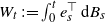 $W_t\,:\!=\int_0^t e_s^\top\,\textrm{d}B_s$
, is a standard Brownian motion in
 ${\mathbb{R}}$
. By the Itô–Meyer formula we get, for all
 $t \lt \tau$
,
 \begin{equation*} \textrm{d}|Z_t| = \frac{1}{|Z_t|}\langle Z_t,b(Y_t^x)-b(\hat{Y}_t)\rangle\,\textrm{d}t + \frac{2|Z_t|}{|\sigma^{-1}Z_t|}\,\textrm{d}W_t \end{equation*}
(note that the local-time part vanishes as
 $t \lt \tau$
, i.e.
 $Z_t\neq 0$
). Since f is piecewise
 $C^2$
and f’ is continuous, we can use Itô’s formula and the expression for
 $\textrm{d}|Z_t|$
to get, for all
 $t \lt \tau$
,
 \begin{equation*} \textrm{d}f(|Z_t|) = \frac{f'(|Z_t|)}{|Z_t|}\langle Z_t,b(Y_t^x)-b(\hat{Y}_t)\rangle\,\textrm{d}t + f''(|Z_t|)\frac{2|Z_t|^2}{|\sigma^{-1}Z_t|^2}\,\textrm{d}t + f'(|Z_t|)\frac{2|Z_t|}{|\sigma^{-1}Z_t|}\,\textrm{d}W_t. \end{equation*}
Since
 $f''\leq0$
on
 $[0,\infty)\setminus\{R_0\}$
and
 $|\sigma^{-1}x| \leq |x|/\lambda_{\min}$
for
 $x\in{\mathbb{R}^d}$
, it follows from (A.1) and Lemma A.1 that
 \begin{align*} \textrm{d}f(|Z_t|) & \leq [f'(|Z_t|)\phi(|Z_t|)+2\lambda_{\min}f''(|Z_t|)]\,\textrm{d}t + f'(|Z_t|)\frac{2|Z_t|}{|\sigma^{-1}Z_t|}\,\textrm{d}W_t \\ & \leq -Cf(|Z_t|)\,\textrm{d}t + f'(|Z_t|)\frac{2|Z_t|}{|\sigma^{-1}Z_t|}\,\textrm{d}W_t, \end{align*}
where
 $C = \frac 12\theta_0f'(R_0)$
. This implies that, for
 $t \lt \tau$
,
 \begin{equation*} \textrm{d}[\textrm{e}^{Ct}f(|Z_t|)] \leq \textrm{e}^{Ct}f'(|Z_t|)\frac{2|Z_t|}{|\sigma^{-1}Z_t|}\,\textrm{d}W_t. \end{equation*}
Using the finite stopping times
 $\tau_n \,:\!= \inf\{t\geq0\colon|Z_t|\notin[1/n,n]\} \leq \tau$
and optional stopping, we see that the right-hand side of the above inequality is a mean-zero martingale. Hence,
 \begin{equation*} \mathbb{E}[\textrm{e}^{C(t\wedge\tau_n)}f(|Z_{t\wedge\tau_n}|)] \leq f(|Z_0|)=f(|x-y|),\quad t\geq 0. \end{equation*}
Since
 $\tau_n\uparrow\tau$
as
 $n\uparrow\infty$
, we can apply Fatou’s lemma and get
 $\mathbb{E}[\textrm{e}^{C(t\wedge\tau)}f(|Z_{t\wedge\tau}|)] \leq f(|x-y|)$
. Noting that
 $Z_t=0$
for
 $t\geq\tau$
and
 $f(0)=0$
, we conclude that
 $\textrm{e}^{Ct}\mathbb{E} f(|Z_t|)\leq f(|x-y|)$
. Because of (A.2), we see that, for all
 $t\geq0$
,
 \begin{equation*} f'(R_0)\mathbb{E}|Y_t^x-\hat{Y}_t| \leq \mathbb{E}f(|Z_t|) \leq \textrm{e}^{-Ct}f(|x-y|) \leq \textrm{e}^{-Ct}|x-y|. \end{equation*}
Since, by construction,
 $\textrm{law}(\hat{Y}_t)=\textrm{law}(Y_t^y)$
, the proof is finished.
Acknowledgements
We would like to thank the anonymous referees for their careful comments and useful suggestions.
Funding information
C.-S. Deng is supported by the National Natural Science Foundation of China (12371149), the Fundamental Research Funds for the Central Universities (Grant No. 2042025kf0020), and the Alexander von Humboldt Foundation. R.L. Schilling is supported by the 6G-Life project (BMFTR Grant No. 16KISK001K) and TU Dresden’s ScaDS.AI initiative. L. Xu is supported by the National Natural Science Foundation of China No. 12071499, the Science and Technology Development Fund (FDCT) of Macau S.A.R. FDCT 0074/2023/RIA2, and the University of Macau grants MYRG2020-00039-FST, MYRG-GRG2023-00088-FST.
Competing interests
There are no competing interests to declare which arose during the preparation process of this article.



