1 Introduction
A major effort in medicine concerns the ability to regulate biochemical processes by controlling for molecular concentration. Living cells sequester biochemical reactions within semi-permeable membrane enveloped compartments and microscopic protein channels transport solutes between compartments (Eisenberg Reference Eisenberg1999; Hille Reference Hille2001). But it is also possible to increase membrane permeability by hybridization. Fusion and lysis, for example, interrupt membrane continuity by forming a macroscopic fluid bridge that connects previously separate aqueous regions (Chang, Chiang & Jackson Reference Chang, Chiang and Jackson2017). There are a number of ways to experimentally disrupt membrane continuity (Riske & Dimova Reference Riske and Dimova2005; Helfield et al. Reference Helfield, Chen, Watkins and Villanueva2016; Sengela & Wallacea Reference Sengela and Wallacea2016), and among these ways illumination and osmotic stress are important techniques because of the impact pressure has on cell shape and uptake of molecules (Manoussaki et al. Reference Manoussaki, Shin, Waterman and Chadwick2015; Arroyo & Trepat Reference Arroyo and Trepat2017).
Leak-out describes the physical process where an increase in cytosolic pressure ruptures the normally intact plasma membrane. To distinguish the forces generating the motion, researchers model leak-out in liposomes (Sandre, Moreaux & Brochard-Wyart Reference Sandre, Moreaux and Brochard-Wyart1999), spherical vesicle compartments enclosing a viscous fluid volume. Experimenters adjust conditions so that the liposome becomes tense and exerts a pressure on its fluid contents. Following nucleation, the rapid expansion of a pore and concomitant pressure driven outflow release energy stored in stretching. The widened pore allows intracellular contents to escape into the aqueous environment and the introduction of exogenous molecules.
To describe leak-out phenomena theoretically, models throughout the literature make the assumption that volumetric outflow rate is directly proportional to membrane tension. The rationale for this assumption is that tension determines the difference in internal and ambient pressures since it is the force responsible for rupture. Fluid should then leak out at a rate proportional to the pressure difference. Because the pore is small, the coefficient of proportionality closely approximates that for a hole in a plane wall. But is it possible, contrary to standard approaches, that tension accounts for only one part of the flow rate?
Sampson calculated the Stokes flow through a hole in plane wall in 1891, giving one of the early examples of fluid flow past a non-convex body. Weissberg (Reference Weissberg1962), Dagan, Weinbaum & Pfeffer (Reference Dagan, Weinbaum and Pfeffer1982) and Jensen, Valente & Stone (Reference Jensen, Valente and Stone2014) extended Sampson’s result to static cylindrical pores and pore distributions. But despite its widespread use in vesicle studies, the accuracy of approximation by Sampson flow has never been theoretically or experimentally tested, mainly due to the fact that the flow fields are unknown for the spherical case.
The spherical cap is a mathematical shape well suited to describing a round liposome with a circular pore. It is a bounded, zero thickness surface containing the disk and plane wall with a hole as limiting cases. Several decades ago, Ranger and coworkers introduced an integral transformation technique called the complementary integral method and determined the steady Stokes flow past the spherical cap (Ranger Reference Ranger1973; Dorrepaal, O’Neill & Ranger Reference Dorrepaal, O’Neill and Ranger1976). At the time, the main results of interest were rheological properties of dilute particle suspensions and studies centred on rigid body motions (Dorrepaal Reference Dorrepaal1978, Reference Dorrepaal1984). Aubin & Ryham (Reference Aubin and Ryham2016) adapted the complementary integral method to a problem where the spherical cap is not rigid, but deforms in the angle defining the pore.
The main theoretical contribution of the present study is a new and exact solution to low Reynolds number flows. The problem in § 4 considers a spherical cap that expels fluid by shrinking in radius. The calculations use the complementary integral method to find an infinite series for the streamfunction and sum the series in elementary form. To realistically model a bursting liposome, the study combines the present Stokes flow solution with prior closed-form results, yielding a general solution whose motions include changes in the spherical radius, as occurs when a liposome expels fluids, changes in the hole angle, replicating the expanding pore, and translation along the axis of revolution. The translation component enables the overall motion to conserve momentum.
Section 6 develops an identity for the rates of energy dissipation of a general, possibly non-axisymmetric surface acting on the fluid. This identity is crucial to determining the resistance coefficients characterizing the hydrodynamic forces and the pressures that arise with a deformable spherical cap. As a direct application, an analysis of the force equation for translation shows that appropriate changes in the spherical radius and hole angle lead to a novel active swimmer locomotion.
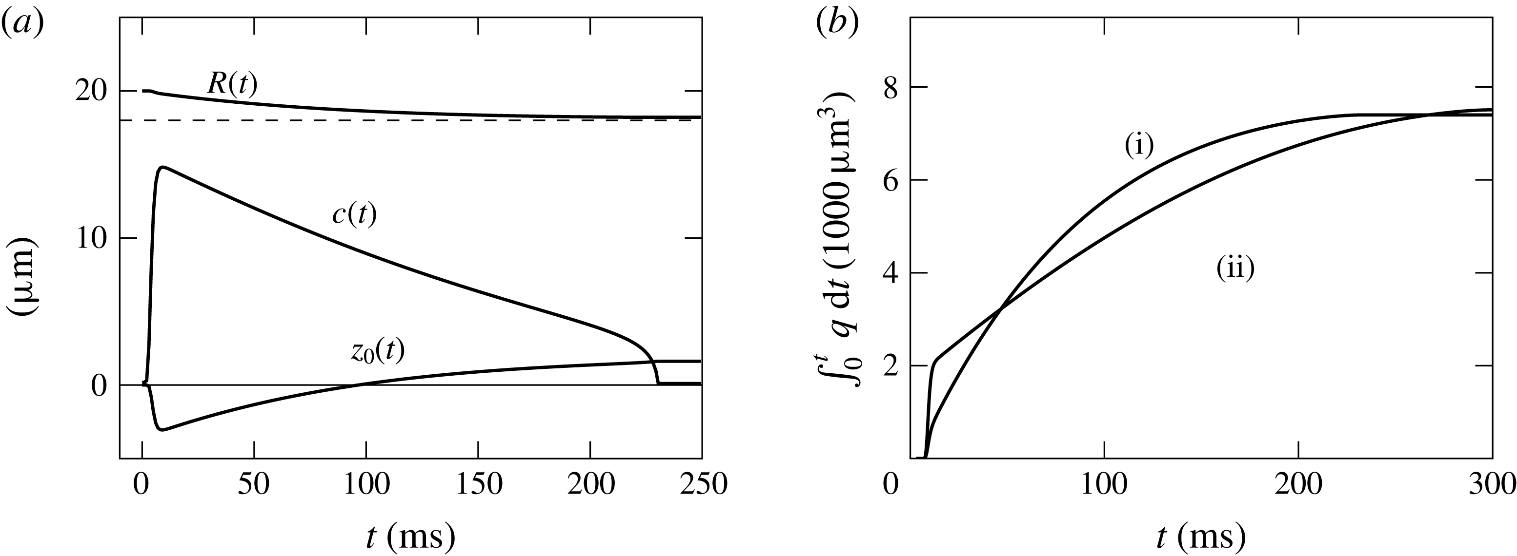
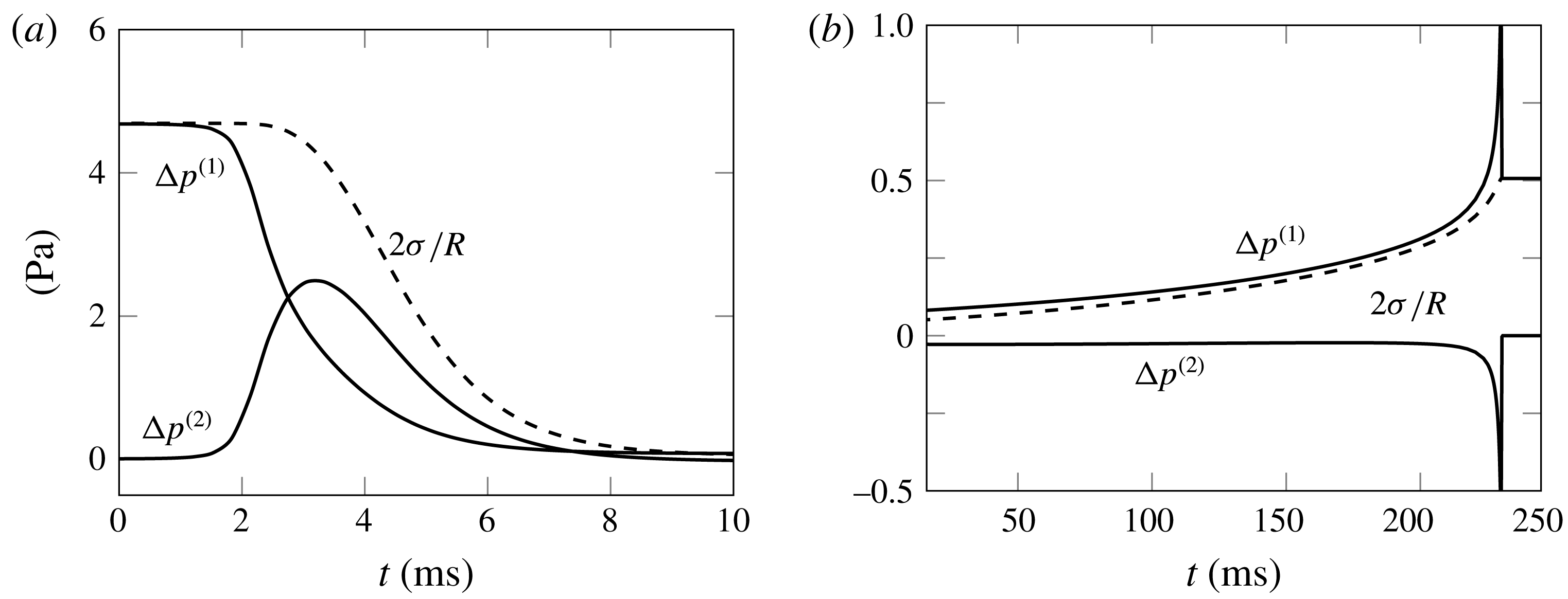
Returning to the biological question that motivated the present study, § 7 proposes a Stokes flow based formulation of pore kinetics. The model uses explicit expressions for the dissipative forces calculated from the closed-form solution to determine pore trajectories. One of the key simulation findings is that by assuming a pressure that depends solely on tension (i.e. one that is independent of pore velocity), models that rely on the Sampson approximation potentially miscalculate the volume of fluid expelled in the process. The reason for this is that during the stage initiating leak-out, the velocity of a rapidly expanding pore contributes roughly the same amount of internal pressure as the tension responsible for rupture. The modified expression for leak-out (7.7) contains the correction to the Sampson relation that appropriately accounts for the rate of hole widening.
2 Problem formulation
Consider a surface
 $\unicode[STIX]{x1D6F4}$
forming the shape of a hollow sphere with a single circular hole. This spherical cap, or calotte, is the portion of the sphere bounded by a circle of latitude:
 $$\begin{eqnarray}\unicode[STIX]{x1D6F4}=\{\boldsymbol{x}\in \mathbb{R}^{3}:r=|\boldsymbol{x}-\boldsymbol{x}_{0}|=R,0\leqslant \unicode[STIX]{x1D703}\leqslant \unicode[STIX]{x1D6FC}\}.\end{eqnarray}$$
The parameter
 $R$
is the spherical radius, the parameter
 $\unicode[STIX]{x1D6FC}$
is the hole angle and
 $(r,\unicode[STIX]{x1D703},\unicode[STIX]{x1D719})$
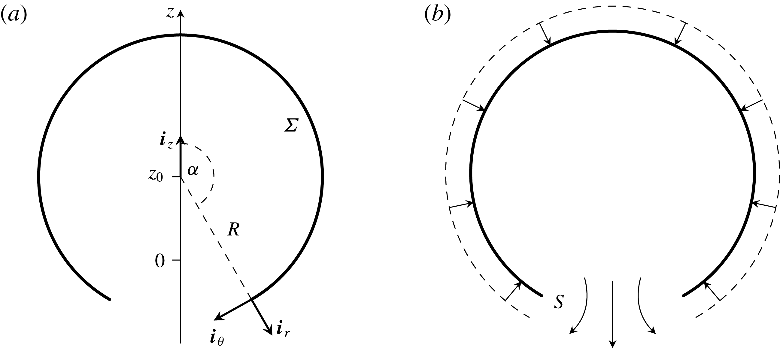
are spherical coordinates (figure 1
a). The centre
 $\boldsymbol{x}_{0}=z_{0}\boldsymbol{i}_{z}$
can move up and down the axis of symmetry. The scalar velocities
 $$\begin{eqnarray}U_{1}=\frac{\text{d}R}{\text{d}t},\quad U_{2}=R\frac{\text{d}\unicode[STIX]{x1D6FC}}{\text{d}t},\quad U_{3}=\frac{\text{d}z_{0}}{\text{d}t},\end{eqnarray}$$
describe the rates of spherical dilation, hole closure and translation along the axis of symmetry, respectively. The spherical cap is rim-less, meaning that stretching and compression of surface area is uniform.
Panel (a) depicts the coordinate vectors and parametrization. In the most basic pattern of leak-out (b), a spherical cap with initially larger radius (dashed arc) contracts to a smaller radius (solid arc). The surface velocity agrees with a sink directed toward the centre. Fluid leaks out through the hole opening
 $S$
(the open part of the sphere) into the ambient aqueous region.

A viscous, incompressible fluid bathes
 $\unicode[STIX]{x1D6F4}.$
Both the inner and outer sides of the surface are in contact with the aqueous region
 $\mathbb{R}^{3}\setminus \unicode[STIX]{x1D6F4}.$
The fluid is steady in the far field and the movements of
 $\unicode[STIX]{x1D6F4}$
drive the liquid. A Stokes boundary value problem describes the fluid motion at low Reynolds number:
 $$\begin{eqnarray}-\unicode[STIX]{x1D707}\unicode[STIX]{x1D6FB}^{2}\boldsymbol{u}+\unicode[STIX]{x1D735}p=0,\quad \operatorname{div}\boldsymbol{u}=0,\quad \text{in }\mathbb{R}^{3}\setminus \unicode[STIX]{x1D6F4},\end{eqnarray}$$
for viscosity
 $\unicode[STIX]{x1D707},$
fluid velocity
 $\boldsymbol{u}$
and fluid pressure
 $p,$
with boundary and far field conditions
 $$\begin{eqnarray}\boldsymbol{u}=U_{1}\boldsymbol{i}_{r}+U_{2}\frac{\tan (\unicode[STIX]{x1D703}/2)}{\tan (\unicode[STIX]{x1D6FC}/2)}\boldsymbol{i}_{\unicode[STIX]{x1D703}}+U_{3}\boldsymbol{i}_{z}\quad \text{on }\unicode[STIX]{x1D6F4},\quad \lim _{r\rightarrow \infty }\boldsymbol{u}=\mathbf{0}.\end{eqnarray}$$
The vectors
 $(\boldsymbol{i}_{r},\boldsymbol{i}_{\unicode[STIX]{x1D703}},\boldsymbol{i}_{\unicode[STIX]{x1D719}})$
are the unit basis for spherical coordinates. The equations (2.3) are the zero Reynolds number, quasi-static, creeping flow approximation. They are the appropriate formulation of the equations of motion for liposome and microscopic swimmer studies where the Reynolds numbers are typically several orders of magnitude smaller than one. The form of (2.4) derives from the fact that the spherical cap is rim-less if and only if the tangential velocity profile is a multiple of
 $\tan (\unicode[STIX]{x1D703}/2)$
(Aubin & Ryham Reference Aubin and Ryham2016). Accordingly, the two-dimensional divergence,
 $$\begin{eqnarray}\text{div}_{\unicode[STIX]{x1D6F4}}\boldsymbol{u}=\unicode[STIX]{x1D735}\boldsymbol{u}\boldsymbol{ : }(\boldsymbol{i}_{\unicode[STIX]{x1D703}}\boldsymbol{i}_{\unicode[STIX]{x1D703}}+\boldsymbol{i}_{\unicode[STIX]{x1D719}}\boldsymbol{i}_{\unicode[STIX]{x1D719}})=\frac{1}{R}\left(2U_{1}+\cot \frac{\unicode[STIX]{x1D6FC}}{2}U_{2}\right)\quad \text{on }\unicode[STIX]{x1D6F4},\end{eqnarray}$$
is independent of
 $\unicode[STIX]{x1D703}.$
The surface
 $\unicode[STIX]{x1D6F4}$
is impervious to the fluid but liquid freely passes across the hole opening
 $$\begin{eqnarray}S=\{\boldsymbol{x}\in \mathbb{R}^{3}:r=R,\unicode[STIX]{x1D6FC}<\unicode[STIX]{x1D703}\leqslant \unicode[STIX]{x03C0}\}.\end{eqnarray}$$
The volumetric leak-out flow rate across
 $S$
is
 $$\begin{eqnarray}q=2\unicode[STIX]{x03C0}R^{2}(\cos \unicode[STIX]{x1D6FC}-1)U_{1}.\end{eqnarray}$$
Note that
 $q$
is positive whenever
 $U_{1}$
is negative (figure 1
b).
The Stokes equations (2.3) are linear in the velocity
 $\boldsymbol{u}$
and pressure
 $p.$
This makes it possible to solve for the boundary values (2.4) by the method of linear superposition of solutions. Let
 $(\boldsymbol{u}^{(i)},p^{(i)}),$
 $i=1,2,3$
be the particular solutions to the Stokes equations (2.3) with the boundary conditions
 $$\begin{eqnarray}\boldsymbol{u}^{(1)}=U_{1}\boldsymbol{i}_{r},\quad \boldsymbol{u}^{(2)}=U_{2}\frac{\tan (\unicode[STIX]{x1D703}/2)}{\tan (\unicode[STIX]{x1D6FC}/2)}\boldsymbol{i}_{\unicode[STIX]{x1D703}},\quad \boldsymbol{u}^{(3)}=U_{3}\boldsymbol{i}_{z},\quad \text{on }\unicode[STIX]{x1D6F4}.\end{eqnarray}$$
That is,
 $(\boldsymbol{u}^{(1)},p^{(1)}),$
 $(\boldsymbol{u}^{(2)},p^{(2)})$
and
 $(\boldsymbol{u}^{(3)},p^{(3)})$
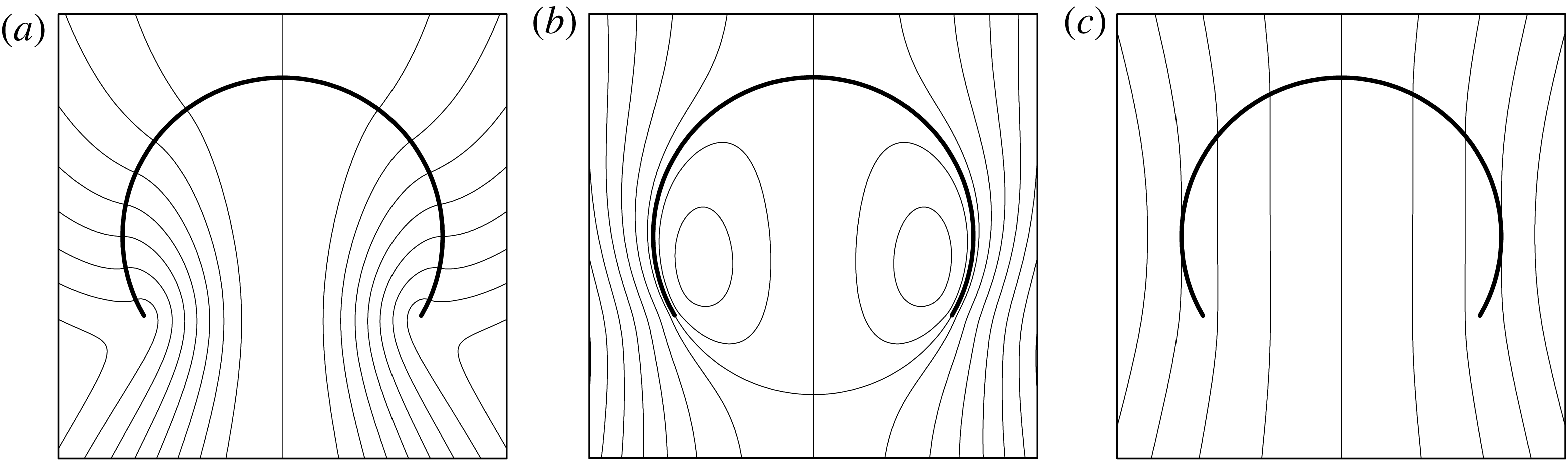
denote the dilation, hole closure and translations components of the motion, respectively (figure 2). Dorrepaal et al. (Reference Dorrepaal, O’Neill and Ranger1976) and Aubin & Ryham (Reference Aubin and Ryham2016) derived closed-form expressions for the motions
 $(\boldsymbol{u}^{(2)},p^{(2)})$
and
 $(\boldsymbol{u}^{(3)},p^{(3)}),$
respectively. The present work gives the calculations for the motion
 $(\boldsymbol{u}^{(1)},p^{(1)}).$
The solution procedure, as outlined in § 4, relies on integral transformation techniques to calculate an infinite series representation for the streamfunction and then sum the series in elementary form. The appendix A gives the explicit formulas for all three cases.
Panels (a–c) show the streamlines for the velocity fields
 $\boldsymbol{u}^{(1)},$
 $\boldsymbol{u}^{(2)}$
and
 $\boldsymbol{u}^{(3)}$
respectively. Accordingly, in panel (a) the streamlines are everywhere perpendicular to the spherical cap and in panel (b) the streamlines are everywhere tangential to the spherical cap. In panel (c) the streamlines intersect
 $\unicode[STIX]{x1D6F4}$
vertically because
 $\boldsymbol{u}^{(3)}=U_{3}\boldsymbol{i}_{z}$
on the spherical cap. The far field is stationary in all three cases.

Summing the boundary conditions (2.8) and applying the linearity of the Stokes equations shows that
 $$\begin{eqnarray}\boldsymbol{u}=\mathop{\sum }_{i=1}^{3}\boldsymbol{u}^{(i)},\quad p=\mathop{\sum }_{i=1}^{3}p^{(i)},\end{eqnarray}$$
3 Main results
In the boundary value problem (2.3), (2.4), the radial velocity kinematically sets the leak-out flow rate
 $q.$
To make physical deductions, it is useful to have a formula that explicitly relates leak-out flow rate to pressure differences. Let
 $$\begin{eqnarray}\unicode[STIX]{x0394}p_{L}=\mathop{\sum }_{i=1}^{3}\unicode[STIX]{x0394}p^{(i)},\quad \unicode[STIX]{x0394}p^{(i)}=p^{(i)}(\boldsymbol{x}_{0})-\lim _{\boldsymbol{x}\rightarrow \infty }p^{(i)}(\boldsymbol{x}),\quad i=1,2,3.\end{eqnarray}$$
The Laplace pressure
 $\unicode[STIX]{x0394}p_{L}$
agrees with the pressure jump across an intact sphere. But in the present study, the sphere has a hole and is no longer intact. It is therefore of interest to know how the pressure difference depends on the flow parameters. The ensuing closed-form solution for (2.9) makes it possible to quantify these jumps in pressure exactly.
The following equation generalizes the Sampson relationship for an unbounded fluid passing through a circular hole in an infinite plane wall to the case of fluid passing through the a hole in a bounded hollow sphere:
 $$\begin{eqnarray}\displaystyle \unicode[STIX]{x0394}p^{(1)} & = & \displaystyle \frac{1}{\unicode[STIX]{x03C0}^{2}}\left[(1-2\cos \unicode[STIX]{x1D6FC})\sin ^{2}\unicode[STIX]{x1D6FC}+\frac{1}{2}\unicode[STIX]{x1D6FC}(11-\cos \unicode[STIX]{x1D6FC})\sin \unicode[STIX]{x1D6FC}\right.\nonumber\\ \displaystyle & & \displaystyle \left.+\,3\unicode[STIX]{x1D6FC}^{2}(2+\cos \unicode[STIX]{x1D6FC})\sin ^{2}\frac{\unicode[STIX]{x1D6FC}}{2}\right]\frac{\unicode[STIX]{x1D707}q}{c^{3}}.\end{eqnarray}$$
The parameter
 $c=R\sin \unicode[STIX]{x1D6FC}$
is the radius of the hole opening. Although valid for
 $0<\unicode[STIX]{x1D6FC}<\unicode[STIX]{x03C0},$
of particular interest are the values of (3.2) in the range of
 $\unicode[STIX]{x1D6FC}$
for which the hole is small in relation to the sphere. At
 $\unicode[STIX]{x1D6FC}=\unicode[STIX]{x03C0},$
(3.2) has the Taylor expansion
 $$\begin{eqnarray}\unicode[STIX]{x0394}p^{(1)}=3\frac{\unicode[STIX]{x1D707}q}{c^{3}}+\frac{3}{4}\frac{\unicode[STIX]{x1D707}q}{c^{3}}(\unicode[STIX]{x1D6FC}-\unicode[STIX]{x03C0})^{2}+O\left(\frac{\unicode[STIX]{x1D707}q}{c^{3}}(\unicode[STIX]{x1D6FC}-\unicode[STIX]{x03C0})^{3}\right).\end{eqnarray}$$
The leading-order term agrees with the expression given by Sampson (Reference Sampson1891) (Happel & Brenner (Reference Happel and Brenner1965), p. 153).
Theoretical studies of membrane poration often use Sampson flow as an idealized model for the overall pressure jump
 $\unicode[STIX]{x0394}p_{L}.$
The basic assumption is that the transversal pressure jump is independent of lateral motion. Although strictly correct for a planar membrane, the assumption ignores the fact that the spherical cap is a finite body. The following expressions for the motions
 $(\boldsymbol{u}^{(2)},p^{(2)})$
and
 $(\boldsymbol{u}^{(3)},p^{(3)})$
show that the integral effect of pressures coming from lateral motion persists even for a small hole:
 $$\begin{eqnarray}\displaystyle & \displaystyle \unicode[STIX]{x0394}p^{(2)}=-12\cot \frac{\unicode[STIX]{x1D6FC}}{2}\left(\unicode[STIX]{x1D6FC}-\sin \unicode[STIX]{x1D6FC}+\unicode[STIX]{x1D6FC}^{2}\tan \frac{\unicode[STIX]{x1D6FC}}{2}\right)\frac{\unicode[STIX]{x1D707}U_{2}}{4\unicode[STIX]{x03C0}R}, & \displaystyle\end{eqnarray}$$
 $$\begin{eqnarray}\displaystyle & \displaystyle \unicode[STIX]{x0394}p^{(3)}=-(6\unicode[STIX]{x1D6FC}+8\sin \unicode[STIX]{x1D6FC}+\sin 2\unicode[STIX]{x1D6FC})\frac{\unicode[STIX]{x1D707}U_{3}}{4\unicode[STIX]{x03C0}R}. & \displaystyle\end{eqnarray}$$
The identity (3.4) has
 $\unicode[STIX]{x0394}p^{(2)}\simeq -3\unicode[STIX]{x03C0}\unicode[STIX]{x1D707}U_{2}/R$
at
 $\unicode[STIX]{x1D6FC}=\unicode[STIX]{x03C0},$
yielding a value that is in some circumstances comparable to the total pressure
 $\unicode[STIX]{x0394}p_{L}.$
This suggests that Sampson flow by itself inadequately characterizes the leak-out process.
3.1 The forces and rates of work of a body acting on the fluid
A central topic in fluid mechanics deals with the forces that a body exerts on its fluid environment. For a single rigid body in a fluid at rest at infinity, the general approach applies a rigid body motion as the velocity boundary condition and determines the rate of work done on the fluid by the rigid motion. The rate of work is quadratic in the translation and torque components, yielding the translation, rotation, and coupling tensors tabulating the interaction coefficients (Happel & Brenner Reference Happel and Brenner1965). For the case of a rigid spherical cap, Ranger (Reference Ranger1973) calculated the torque for a non-axisymmetric streaming flow perpendicular to the axis of rotation. Dorrepaal (Reference Dorrepaal1978, Reference Dorrepaal1984) determined the fundamental resistance tensors and analysed the motion of a spherical cap in shear flow. Crowdy (Reference Crowdy2016) derived the Jeffery equations for an arc geometry similar to the spherical cap in two dimensional shear flow.
The resistance tensor approach adopted in the present study is analogous to that for rigid bodies. The main difference being that instead of applying boundary conditions for a rigid body motion, I apply boundary conditions for a deformable body. The axisymmetric flow is torque free and steady in the far field. The spherical cap has the state variables
 $R,$
 $\unicode[STIX]{x1D6FC}$
and
 $z_{0}$
along with the parameters
 $U_{1},$
 $U_{2}$
and
 $U_{3}$
that control the rates of change in
 $R,$
 $\unicode[STIX]{x1D6FC}$
and
 $z_{0}$
independently. The motions
 $(\boldsymbol{u}^{(1)},p^{(1)}),$
 $(\boldsymbol{u}^{(2)},p^{(2)})$
and
 $(\boldsymbol{u}^{(3)},p^{(3)})$
that make up the superposition solution (2.9) are proportional to their respective values for
 $U_{i},$
 $i=1,2,3.$
Viscous dissipations limit the movements of the spherical cap. The rate of work is quadratic in the parameters
 $U_{i},$
 $i=1,2,3$
and scales with the viscosity
 $\unicode[STIX]{x1D707}$
and
 $R.$
This motivates the following definition for the dimensionless resistance coefficients
 $[F_{ij}]:$
 $$\begin{eqnarray}\unicode[STIX]{x1D707}RF_{ij}U_{i}U_{j}=\int _{\unicode[STIX]{x1D6F4}}[\boldsymbol{u}^{(i)}\boldsymbol{\cdot }\unicode[STIX]{x1D64F}^{(j)}\boldsymbol{\cdot }\text{d}\boldsymbol{S}]_{\pm },\quad i,j=1,2,3.\end{eqnarray}$$
Here
 $\unicode[STIX]{x1D64F}^{(j)}=-\boldsymbol{I}p^{(j)}+2\unicode[STIX]{x1D707}\unicode[STIX]{x1D750}^{(j)}$
and
 $\unicode[STIX]{x1D750}^{(j)}=[\unicode[STIX]{x1D735}\boldsymbol{u}^{(j)}+(\unicode[STIX]{x1D735}\boldsymbol{u}^{(j)})^{\text{T}}]/2$
are the dyadic stress tensor and rate of deformation tensor for the motion
 $(\boldsymbol{u}^{(j)},p^{(j)})$
(Leal Reference Leal2006). The area element is
 $\text{d}\boldsymbol{S}=\boldsymbol{i}_{r}\text{d}S$
and the operation
 $[(\cdot )]_{\pm }=\lim _{r\rightarrow R^{-}}(\cdot )-\lim _{r\rightarrow R^{+}}(\cdot )$
accounts for the net rate of work performed by the inner and outer leaflets of
 $\unicode[STIX]{x1D6F4}$
respectively. By the Lorentz reciprocal identity, the coefficients form a symmetric tensor:
 $$\begin{eqnarray}\mathit{F}_{ij}=\mathit{F}_{ji},\quad i,j=1,2,3.\end{eqnarray}$$
Fundamental fluid mechanical quantities follow from the definition (3.6). The dissipation function
 ${\mathcal{E}}$
quantifies the rate energy of dissipation for the motion
 $\boldsymbol{u}=\sum _{i=1}^{3}\boldsymbol{u}^{(i)},$
 $p=\sum _{i=1}^{3}p^{(i)}$
due to viscous losses in the aqueous phase. It takes the various forms (Happel & Brenner Reference Happel and Brenner1965)
 $$\begin{eqnarray}\displaystyle {\mathcal{E}} & = & \displaystyle \int _{\mathbb{R}^{3}}2\unicode[STIX]{x1D707}\unicode[STIX]{x1D750}\boldsymbol{ : }\unicode[STIX]{x1D750}\,\text{d}x=\int _{\unicode[STIX]{x1D6F4}}[\boldsymbol{u}\boldsymbol{\cdot }\unicode[STIX]{x1D64F}\boldsymbol{\cdot }\text{d}\boldsymbol{S}]_{\pm }\nonumber\\ \displaystyle & = & \displaystyle \mathop{\sum }_{i,j=1}^{3}\int _{\unicode[STIX]{x1D6F4}}[\boldsymbol{u}^{(i)}\boldsymbol{\cdot }\unicode[STIX]{x1D64F}^{(j)}\boldsymbol{\cdot }\text{d}\boldsymbol{S}]_{\pm }=\mathop{\sum }_{i,j=1}^{3}\unicode[STIX]{x1D707}R\mathit{F}_{ij}U_{i}U_{j}.\end{eqnarray}$$
The dyadics
 $\unicode[STIX]{x1D750}$
and
 $\unicode[STIX]{x1D64F}$
are for the motion
 $(\boldsymbol{u},p)$
.
To derive kinetic equations, suppose that the spherical cap has the internal energy
 $W(R,\unicode[STIX]{x1D6FC},z_{0}).$
A liposome with a single pore, for example, has the internal energy of mechanical stretching and edge energy of the pore. In any event, the principle of maximum dissipation states that the dissipative force (one half the gradient in dissipation with respect to velocity) balances the conservative force (the gradient in internal energy) (Strutt Reference Strutt1871; Onsager Reference Onsager1931a
,Reference Onsager
b
; Martínez-Balbuena, Hernández-Zapata & Santamaría-Holek Reference Martínez-Balbuena, Hernández-Zapata and Santamaría-Holek2015):
 $$\begin{eqnarray}{\textstyle \frac{1}{2}}\unicode[STIX]{x1D735}_{U}{\mathcal{E}}+\unicode[STIX]{x1D735}W=0.\end{eqnarray}$$
Expressing (3.9) component-wise yields a system of linear equations in the velocity parameters
 $U_{i},$
 $i=1,2,3.$
Solving for the velocity parameters yields a set of ordinary differential equations in the parameters
 $R,$
 $\unicode[STIX]{x1D6FC}$
and
 $z_{0}.$
The components of the system (3.9) contain the dissipative part of the force,
 $$\begin{eqnarray}F_{i}=\frac{1}{2}\frac{\unicode[STIX]{x2202}{\mathcal{E}}}{\unicode[STIX]{x2202}U_{i}}=\unicode[STIX]{x1D707}R(F_{i1}U_{1}+F_{i2}U_{2}+F_{i3}U_{3}),\quad i=1,2,3,\end{eqnarray}$$
of the surface acting on the fluid in the direction of the
 $i$
th state variable: here,
 $R,$
 $\unicode[STIX]{x1D6FC}$
and
 $z_{0}$
are the first, second and third state variable, respectively.
To make use of (3.9), it is necessary to determine the nine entries of the coefficient matrix
 $[\mathit{F}_{ij}].$
Actually, the symmetry relations (3.7) reduce this determination to six unknowns. The coefficient
 $F_{33}$
is the drag coefficient for axisymmetric streaming flow past the spherical cap. Dorrepaal et al. (Reference Dorrepaal, O’Neill and Ranger1976) furnish the value
 $$\begin{eqnarray}F_{33}=6\unicode[STIX]{x1D6FC}+8\sin \unicode[STIX]{x1D6FC}+\sin 2\unicode[STIX]{x1D6FC},\quad 0<\unicode[STIX]{x1D6FC}<\unicode[STIX]{x03C0}.\end{eqnarray}$$
This expression contains the drag coefficient for the sphere (
 $\unicode[STIX]{x1D6FC}\rightarrow \unicode[STIX]{x03C0}$
) and the disk (
 $\unicode[STIX]{x1D6FC}\rightarrow 0$
) as limiting cases. Aubin & Ryham (Reference Aubin and Ryham2016) derived the value of the second diagonal coefficient:
 $$\begin{eqnarray}F_{22}=8\cot ^{2}\frac{\unicode[STIX]{x1D6FC}}{2}\left(\unicode[STIX]{x1D6FC}-\sin \unicode[STIX]{x1D6FC}+\unicode[STIX]{x1D6FC}^{2}\tan \frac{\unicode[STIX]{x1D6FC}}{2}\right),\quad 0<\unicode[STIX]{x1D6FC}<\unicode[STIX]{x03C0},\end{eqnarray}$$
where
 ${\mathcal{C}}=F_{22}/(2\unicode[STIX]{x03C0}\sin \unicode[STIX]{x1D6FC}),$
in their notation, denotes the aqueous drag coefficient for pore velocity.
The remainder of this section gives the four remaining and formerly undetermined coefficients
 $F_{11},$
 $F_{12},$
 $F_{13}$
and
 $F_{23}.$
The calculation of force acting in the positive
 $z$
-direction gives the value of the coefficient
 $F_{23}$
(see the remark following (4.24)). Section 6.1 contains the relevant derivation for the radial resistance coefficients
 $F_{11},$
 $F_{12}$
and
 $F_{13}.$
Crucial to these derivations is the following identity, developed in § 6, for the rate of work of the surface acting on the fluid through dilation or contraction:
 $$\begin{eqnarray}\int _{\unicode[STIX]{x1D6F4}}[\boldsymbol{u}^{(1)}\boldsymbol{\cdot }\unicode[STIX]{x1D64F}^{(j)}\boldsymbol{\cdot }\text{d}\boldsymbol{S}]_{\pm }=-4\unicode[STIX]{x03C0}R^{2}U_{1}\unicode[STIX]{x0394}p^{(j)},\quad j=1,2,3.\end{eqnarray}$$
The left-hand side equals
 $\unicode[STIX]{x1D707}RF_{1j}U_{1}U_{j},$
 $j=1,2,3,$
showing that the jumps in pressure
 $\unicode[STIX]{x0394}p^{(j)}$
determine the values for
 $F_{1j}.$
That is why § 5 introduces an analytical method for calculating the pressure field. The identity (3.13) is analogous to the expression for the additional jump in pressure due to the presence of a particle suspension in an infinitely long cylinder (Brenner Reference Brenner1958), and generalizes to surfaces of arbitrary shape.
Following (3.13), the force acting in the radial direction is
 $$\begin{eqnarray}\displaystyle F_{1} & = & \displaystyle \unicode[STIX]{x1D707}R(F_{11}U_{1}+F_{12}U_{2}+F_{13}U_{3})\nonumber\\ \displaystyle & = & \displaystyle -4\unicode[STIX]{x03C0}R^{2}(\unicode[STIX]{x0394}p^{(1)}+\unicode[STIX]{x0394}p^{(2)}+\unicode[STIX]{x0394}p^{(3)}).\end{eqnarray}$$
If
 $U_{1}$
is negative and
 $U_{2}$
and
 $U_{3}$
are zero, then (3.14) is equivalent to the force exerted on a rigid obstruction
 $\unicode[STIX]{x1D6F4}$
by a sink flow with volumetric flow rate
 $4\unicode[STIX]{x03C0}U_{1}R^{2}.$
Lateral stresses arise due to the tangential part of the no-slip condition (2.4), as well as the radial and translation parts of the motion:
 $$\begin{eqnarray}\displaystyle F_{2} & = & \displaystyle \unicode[STIX]{x1D707}R(F_{21}U_{1}+F_{22}U_{2}+F_{23}U_{3})\nonumber\\ \displaystyle & = & \displaystyle \unicode[STIX]{x1D707}R\left[\cot \frac{\unicode[STIX]{x1D6FC}}{2}\left(\unicode[STIX]{x1D6FC}-\sin \unicode[STIX]{x1D6FC}+\unicode[STIX]{x1D6FC}^{2}\tan \frac{\unicode[STIX]{x1D6FC}}{2}\right)\left(12U_{1}+8\cot \frac{\unicode[STIX]{x1D6FC}}{2}U_{2}\right)\right.\nonumber\\ \displaystyle & & \displaystyle +\left.\cot \frac{\unicode[STIX]{x1D6FC}}{2}(\sin 2\unicode[STIX]{x1D6FC}+4\unicode[STIX]{x1D6FC}\cos \unicode[STIX]{x1D6FC}-2\unicode[STIX]{x1D6FC}-4\sin \unicode[STIX]{x1D6FC})U_{3}\right].\end{eqnarray}$$
Consistent with the reciprocal identity, note how the coefficients for
 $U_{1}$
and
 $U_{3}$
in (3.15) mirror the coefficients in (3.14) and the subsequent (3.16), respectively.
A freely suspended spherical cap conserves linear momentum. It is therefore important to have the force
 $F_{3}$
acting parallel to the axis of revolution:
 $$\begin{eqnarray}\displaystyle F_{3} & = & \displaystyle \unicode[STIX]{x1D707}R(F_{31}U_{1}+F_{32}U_{2}+F_{33}U_{3})\nonumber\\ \displaystyle & = & \displaystyle \unicode[STIX]{x1D707}R\left[(6\unicode[STIX]{x1D6FC}+8\sin \unicode[STIX]{x1D6FC}+\sin 2\unicode[STIX]{x1D6FC})(U_{1}+U_{3})\right.\nonumber\\ \displaystyle & & \displaystyle +\left.\cot \frac{\unicode[STIX]{x1D6FC}}{2}(\sin 2\unicode[STIX]{x1D6FC}+4\unicode[STIX]{x1D6FC}\cos \unicode[STIX]{x1D6FC}-2\unicode[STIX]{x1D6FC}-4\sin \unicode[STIX]{x1D6FC})U_{2}\right].\end{eqnarray}$$
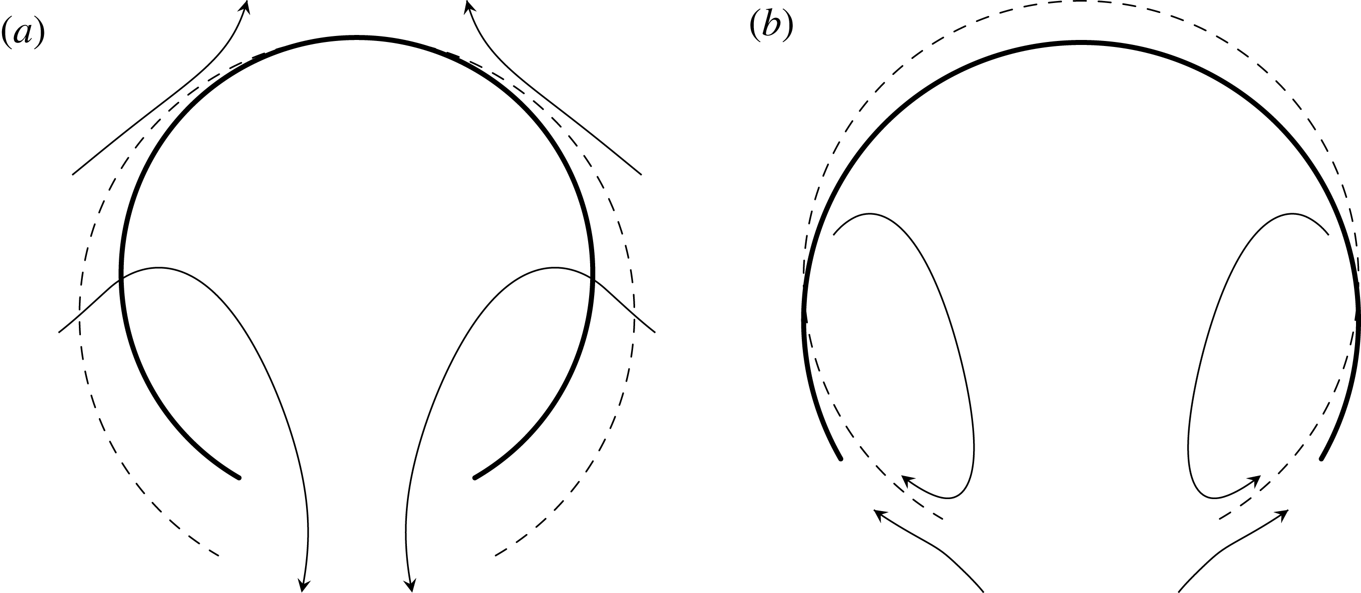
As an illustration, equation (3.16) states that a deflating spherical cap tends to stay in place whenever the hole angle is fixed (figure 3
a, supplementary movie 1 available online at https://doi.org/10.1017/jfm.2017.807). To see this, consider a fluid sphere under interfacial tension (Reyssat & Quéré Reference Reyssat and Quéré2006) with a solid ring attached to the interface. Assume that
 $U_{2}$
is zero, since the hole angle is essentially constant when the ring diameter is sufficiently small. Puncturing the spanning film allows fluid to escape under the action of tension (Jackson & Sleyman Reference Jackson and Sleyman2010). In the absence of any external influence,
 $F_{3}=0$
and it follows from (3.16) that
 $U_{1}+U_{3}$
must be zero.
The diagrams depict how a freely suspended spherical cap translates along the axis of symmetry to conserve ambient fluid momentum. (a) For a fixed hole angle, the aft part of the sphere advances exactly twice the change in spherical radius and the fore part of the spherical cap is a stagnation point. (b) For a fixed spherical radius, hole widening and circulation draw the fore part of the spherical downward.

In light-triggered bursting of vesicles, for example, it is helpful to the observation that the vesicles remain within the field of view (Lira et al.
Reference Lira, Steinkühler, Knorr, Dimova and Riske2016; Peyret et al.
Reference Peyret, Ibarboure, Tron, Beauté, Rust, Sandre, McClenaghan and Lecommandoux2017). Perhaps the stationarity implied by (3.16) offers a plausible explanation as to why bursting vesicles do not propel uncontrollably out of the focal plane. More generally, the coefficient for
 $U_{2}$
in (3.16) is negative while the coefficient for
 $U_{1}+U_{3}$
is positive. The physical interpretation of this sign difference is that hole widening tends to draw the fore part of the spherical cap backward (figure 3
b, supplementary movie 2).
3.2 Locomotion for a spherical cap swimmer
The preliminary analysis of the term
 $F_{3}$
reveals that the translation force transmitted by spherical contraction and hole closure pushes the spherical cap a finite distance along the axis of revolution (figure 3). But at zero Reynolds number, a dilation reverting the contraction, for example, moves the shape back to its original position because the motion uses only one degree of freedom – the spherical radius
 $R$
(Purcell Reference Purcell1977). This raises the question of whether it is possible to define a cyclic shape deformation that utilizes both degrees of freedom, radius and angle, to turn the spherical cap into a swimmer.
To study the matter conceptually, consider a piecewise deformation initiated by a contraction
 $(a)$
, moving the centre a distance forward, followed by a hole widening
 $(b)$
moving the centre backwards (figure 4). To bring the spherical cap back to its original shape, continue with a dilation
 $(a^{\prime })$
followed by a hole closure
 $(b^{\prime })$
. The overall sequence of moves
 $aba^{\prime }b^{\prime }$
is irreversible because
 $aba^{\prime }b^{\prime }\neq bab^{\prime }a^{\prime }$
. It results in locomotion because the hole widening step
 $(b)$
occurred at a smaller radius than that of the final hole closure step
 $(b^{\prime })$
.
To illustrate the locomotion mathematically, let
 $R(t)$
and
 $\unicode[STIX]{x1D6FC}(t)$
be
 $T$
-periodic functions, modelling cyclic motion of an active spherical cap swimmer. Under the absence of external forces, it holds that
 $$\begin{eqnarray}0=F_{31}\left(\frac{\text{d}R}{\text{d}t}+\frac{\text{d}z_{0}}{\text{d}t}\right)+F_{32}R\frac{\text{d}\unicode[STIX]{x1D6FC}}{\text{d}t},\quad 0\leqslant t<\infty ,\end{eqnarray}$$
where
 $F_{31}=F_{33}$
and
 $F_{32}$
are the coefficients from (3.16). Equation (3.17) gives rise to non-time-reversible effects arise due to the factor
 $R$
appearing in front of the time derivative
 $\text{d}\unicode[STIX]{x1D6FC}/\text{d}t;$
the force magnitude delivered by changes in the hole angle depends on the radius. Solving for
 $\text{d}z_{0}/\text{d}t,$
integrating over the period
 $t\in [0,T]$
and using
 $R(T)=R(0)$
implies that
 $$\begin{eqnarray}z_{0}(T)-z_{0}(0)=-\int _{0}^{T}R(t)\frac{F_{32}(\unicode[STIX]{x1D6FC}(t))}{F_{31}(\unicode[STIX]{x1D6FC}(t))}\frac{\text{d}\unicode[STIX]{x1D6FC}}{\text{d}t}\,\text{d}t.\end{eqnarray}$$
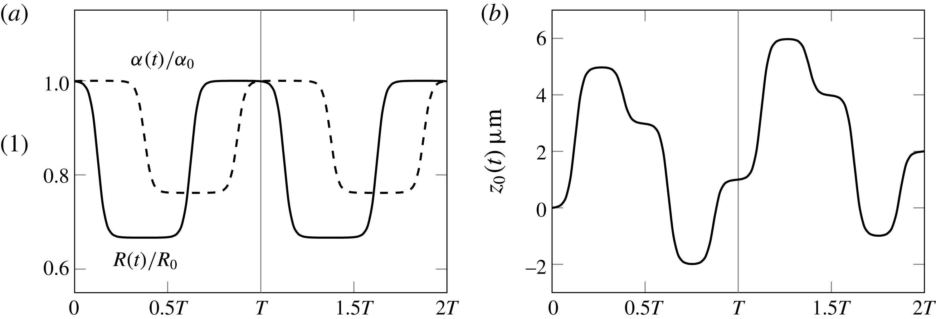
The dynamic shape deformations yield locomotion whenever the integral in (3.18) is positive. Figure 5 illustrates the locomotive process over two periods.
The dashed and solid arcs illustrate sequential shape changes that lead to spherical cap swimming. The filled circle marks the translated centre in reference to the original centre (
 $+$
).

In (a), the spherical radius circulates between the values
 $R_{0}=15~\unicode[STIX]{x03BC}\text{m}$
and
 $R_{1}=10~\unicode[STIX]{x03BC}\text{m}$
while the hole angle circulates between the values
 $\unicode[STIX]{x1D6FC}_{0}=160^{\circ }$
and
 $\unicode[STIX]{x1D6FC}_{1}=120^{\circ }$
over a period
 $T$
(grey, vertical line). The transitions in
 $R(t)$
and
 $\unicode[STIX]{x1D6FC}(t)$
are staggered by a quarter of the period. In (b), after two periods, the shape of the spherical cap is the same as at
 $t=0$
but the net translation of the centre (3.18) is about
 $2~\unicode[STIX]{x03BC}\text{m}$
.

Locomotion for the arc and disc geometries appears in other contexts as well. Lauga & Davis (Reference Lauga and Davis2012) calculate the Marangoni propulsion for a circular disk using integral transformation techniques very similar to the ones employed in the present work (see § 4.1 of the present work). The spherical cap also resembles the bi-concave vesicle studied in Evans, Spagnolie & Lauga (Reference Evans, Spagnolie and Lauga2010), where the authors exploit changes in surface and volume composition to generate propulsion.
4 A spherical cap changing in size
The explicit expressions for pressure and force from § 3 derive from closed-form solutions to Stokes boundary value problems for the spherical cap. Dorrepaal et al. (Reference Dorrepaal, O’Neill and Ranger1976) and Aubin & Ryham (Reference Aubin and Ryham2016) derived the motions
 $(\boldsymbol{u}^{(3)},p^{(3)})$
and
 $(\boldsymbol{u}^{(2)},p^{(2)})$
for the case of translation parallel to the axis of revolution and changes in the hole angle, respectively. The goal of the present section is to derive the leak-out motion
 $(\boldsymbol{u}^{(1)},p^{(1)})$
for changes in the spherical radius, thereby completing the superposition solution (2.9).
To outline the approach, the calculations cast the axisymmetric equations of motion as a single fourth-order scalar equation for the streamfunction. The solution of the streamfunction equation proceeds by the method of separation of variables and expresses the series solution in closed form using a set of generating functions. This yields the velocity
 $\boldsymbol{u}^{(1)}.$
To derive the pressure
 $p^{(1)}$
, § 5 introduces an analytical technique for explicitly calculating the pressure field in terms of the streamfunction generating function representation. Neither Dorrepaal et al. (Reference Dorrepaal, O’Neill and Ranger1976) nor Aubin & Ryham (Reference Aubin and Ryham2016) attempted a calculation of the pressure to this level of detail.
In the leak-out motion
 $(\boldsymbol{u}^{(1)},p^{(1)}),$
the spherical radius of the surface
 $\unicode[STIX]{x1D6F4}$
is changing with rate
 $U_{1}$
but the hole angle and centre relative to the far field are constant. This corresponds to setting
 $U_{2}=U_{3}=0$
in (2.3), (2.4), yielding the boundary value problem
 $$\begin{eqnarray}-\unicode[STIX]{x1D707}\unicode[STIX]{x1D6FB}^{2}\boldsymbol{u}+\unicode[STIX]{x1D735}p=0,\quad \operatorname{div}\boldsymbol{u}=0,\quad \text{in }\mathbb{R}^{3}\setminus \unicode[STIX]{x1D6F4},\end{eqnarray}$$
with boundary and far field conditions
 $$\begin{eqnarray}\boldsymbol{u}=U_{1}\boldsymbol{i}_{r}\quad \text{on }\unicode[STIX]{x1D6F4},\quad \lim _{r\rightarrow \infty }\boldsymbol{u}=\mathbf{0}.\end{eqnarray}$$
Since the flow is axisymmetric, a streamfunction
 $\unicode[STIX]{x1D713}$
prescribes the fluid velocity:
 $$\begin{eqnarray}u_{r}(r,\unicode[STIX]{x1D703})=-\frac{U_{1}R^{2}}{r^{2}\sin \unicode[STIX]{x1D703}}\frac{\unicode[STIX]{x2202}}{\unicode[STIX]{x2202}\unicode[STIX]{x1D703}}\left[\unicode[STIX]{x1D713}\left(\frac{r}{R},\unicode[STIX]{x1D703}\right)\right],\quad u_{\unicode[STIX]{x1D703}}(r,\unicode[STIX]{x1D703})=\frac{U_{1}R^{2}}{r\sin \unicode[STIX]{x1D703}}\frac{\unicode[STIX]{x2202}}{\unicode[STIX]{x2202}r}\left[\unicode[STIX]{x1D713}\left(\frac{r}{R},\unicode[STIX]{x1D703}\right)\right],\quad u_{\unicode[STIX]{x1D719}}\equiv 0.\end{eqnarray}$$
The scaling in (4.3) makes
 $\unicode[STIX]{x1D713}$
dimensionless and the streamfunction satisfies
 $$\begin{eqnarray}\left\{\begin{array}{@{}ll@{}}\displaystyle E^{4}\unicode[STIX]{x1D713}=0, & \\ \displaystyle \unicode[STIX]{x1D713}(1,\unicode[STIX]{x1D703})=\cos \unicode[STIX]{x1D703}-1, & 0\leqslant \unicode[STIX]{x1D703}\leqslant \unicode[STIX]{x1D6FC},\\ \displaystyle \unicode[STIX]{x2202}_{r}\unicode[STIX]{x1D713}(1,\unicode[STIX]{x1D703})=0, & 0\leqslant \unicode[STIX]{x1D703}\leqslant \unicode[STIX]{x1D6FC}.\end{array}\right.\end{eqnarray}$$
The geometry for the boundary value problem (4.4) is the same as for figure 1 with the radius
 $R$
scaled to unity. Here
 $E^{4}=(E^{2})^{2}$
and
 $E^{2}$
stands for the Stokes operator (Happel & Brenner Reference Happel and Brenner1965, p. 105):
 $$\begin{eqnarray}E^{2}=\frac{\unicode[STIX]{x2202}^{2}}{\unicode[STIX]{x2202}r^{2}}+\frac{\sin \unicode[STIX]{x1D703}}{r^{2}}\frac{\unicode[STIX]{x2202}}{\unicode[STIX]{x2202}\unicode[STIX]{x1D703}}\left(\frac{1}{\sin \unicode[STIX]{x1D703}}\frac{\unicode[STIX]{x2202}}{\unicode[STIX]{x2202}\unicode[STIX]{x1D703}}\right).\end{eqnarray}$$
The formulation (4.4) takes boundary values at
 $r=1,$
making it convenient to look for a streamfunction of the form (Dorrepaal et al.
Reference Dorrepaal, O’Neill and Ranger1976)
 $$\begin{eqnarray}\unicode[STIX]{x1D713}={\textstyle \frac{1}{2}}(r^{2}-1)r\unicode[STIX]{x2202}_{r}V_{1}-V_{1}-(r^{2}-1)V_{2}.\end{eqnarray}$$
This solution form transforms the fourth-order mixed boundary value problem (4.4) into a system of second-order elliptic problems. Substitution shows that (4.6) satisfies (4.4) provided
 $$\begin{eqnarray}\left\{\begin{array}{@{}ll@{}}\displaystyle E^{2}V_{1}=0, & E^{2}V_{2}=0,\\ \displaystyle V_{1}(1,\unicode[STIX]{x1D703})=1-\cos \unicode[STIX]{x1D703}, & V_{2}(1,\unicode[STIX]{x1D703})=0,0\leqslant \unicode[STIX]{x1D703}\leqslant \unicode[STIX]{x1D6FC}.\end{array}\right.\end{eqnarray}$$
The system of elliptic problems has a unique solution provided the velocity
 $\boldsymbol{u}$
is bounded. To avoid confusion, note that the subscripts in (4.6) are unrelated to those of the scalar velocities (2.2) from § 2.
4.1 Streamfunction
The separation of variables solution of the Stokes operator equation
 $E^{2}V_{j}=0$
is
 $$\begin{eqnarray}V_{j}(r,\unicode[STIX]{x1D703})=\mathop{\sum }_{n=1}^{\infty }A_{n}^{(j)}r^{n+1}{\mathcal{Q}}_{n}(\cos \unicode[STIX]{x1D703}),\quad r\leqslant 1,j=1,2,\end{eqnarray}$$
where
 ${\mathcal{Q}}_{n}(x)=P_{n-1}(x)-P_{n+1}(x)$
and
 $P_{n}(x)$
are Legendre polynomials (Leal Reference Leal2006). (The notation for
 ${\mathcal{Q}}_{n}$
uses a scripted font in order to distinguish it from the second solution
 $Q_{n}$
of the Legendre equation.) The inversion formula
 $$\begin{eqnarray}V_{j}(r,\unicode[STIX]{x1D703})=rV_{j}(r^{-1},\unicode[STIX]{x1D703}),\quad 0<r<\infty ,j=1,2,\end{eqnarray}$$
supplies the values of
 $V_{j},$
 $j=1,2$
for
 $r>1.$
To calculate the Fourier–Legendre coefficients
 $A_{n}^{(j)},$
I employ an integral transformation technique called the complementary integral method (Ranger Reference Ranger1973). At issue is the absence of boundary data for
 $\unicode[STIX]{x1D703}\in (\unicode[STIX]{x1D6FC},\unicode[STIX]{x03C0}]$
(the open part of the sphere
 $S$
) in the formulation (4.4). The complementary integral method overcomes this difficulty by realizing the coefficients
 $A_{n}^{(j)}$
in terms of an appropriate Fourier sine series.
Define the conjugate harmonic functions
 $$\begin{eqnarray}w_{j}(r,\unicode[STIX]{x1D706})+\text{i}v_{j}(r,\unicode[STIX]{x1D706})=\frac{2^{3/2}}{\unicode[STIX]{x03C0}}\mathop{\sum }_{n=1}^{\infty }A_{n}^{(j)}(r\text{e}^{\text{i}\unicode[STIX]{x1D706}})^{n+1/2},\quad r\leqslant 1,j=1,2.\end{eqnarray}$$
Applying the Mehler–Dirichlet integrals (Whittaker & Watson Reference Whittaker and Watson2006) to (4.8) yields the integral representations
 $$\begin{eqnarray}V_{j}(r,\unicode[STIX]{x1D703})=r^{1/2}\int _{0}^{\unicode[STIX]{x1D703}}\frac{v_{j}(r,\unicode[STIX]{x1D706})\sin \unicode[STIX]{x1D706}}{\sqrt{\cos \unicode[STIX]{x1D706}-\cos \unicode[STIX]{x1D703}}}\,\text{d}\unicode[STIX]{x1D706}=-r^{1/2}\int _{\unicode[STIX]{x1D703}}^{\unicode[STIX]{x03C0}}\frac{w_{j}(r,\unicode[STIX]{x1D706})\sin \unicode[STIX]{x1D706}}{\sqrt{\cos \unicode[STIX]{x1D703}-\cos \unicode[STIX]{x1D706}}}\,\text{d}\unicode[STIX]{x1D706},\end{eqnarray}$$
for
 $0\leqslant r\leqslant 1$
and
 $j=1,2.$
To calculate the values of
 $v_{j}(1,\unicode[STIX]{x1D706})$
on the interval
 $[0,\unicode[STIX]{x1D6FC}],$
substitute the boundary data from (4.7) into (4.11). These substitutions form two integral equations of Abel type (Bocher Reference Bocher1926):
 $$\begin{eqnarray}1-\cos \unicode[STIX]{x1D703}=\int _{0}^{\unicode[STIX]{x1D703}}\frac{v_{1}(1,\unicode[STIX]{x1D706})\sin \unicode[STIX]{x1D706}}{\sqrt{\cos \unicode[STIX]{x1D706}-\cos \unicode[STIX]{x1D703}}}\,\text{d}\unicode[STIX]{x1D706},\quad 0=\int _{0}^{\unicode[STIX]{x1D703}}\frac{v_{2}(1,\unicode[STIX]{x1D706})\sin \unicode[STIX]{x1D706}}{\sqrt{\cos \unicode[STIX]{x1D706}-\cos \unicode[STIX]{x1D703}}}\,\text{d}\unicode[STIX]{x1D706},\end{eqnarray}$$
for
 $0\leqslant \unicode[STIX]{x1D703}\leqslant \unicode[STIX]{x1D6FC}.$
Solving the integral equations gives
 $$\begin{eqnarray}v_{1}(1,\unicode[STIX]{x1D706})=2^{3/2}\unicode[STIX]{x03C0}^{-1}\sin \frac{\unicode[STIX]{x1D706}}{2},\quad v_{2}(1,\unicode[STIX]{x1D706})=0,\quad 0\leqslant \unicode[STIX]{x1D706}\leqslant \unicode[STIX]{x1D6FC}.\end{eqnarray}$$
The Stokes equation
 $E^{4}\unicode[STIX]{x1D713}=0$
holds everywhere in the aqueous region and requires that
 $\unicode[STIX]{x2202}_{r}^{k}\unicode[STIX]{x1D713}(r,\unicode[STIX]{x1D703})$
be continuous at
 $r=1$
for
 $\unicode[STIX]{x1D6FC}<\unicode[STIX]{x1D703}\leqslant \unicode[STIX]{x03C0}$
and orders
 $k=0,1,2,3,4.$
The functions
 $\unicode[STIX]{x1D713}$
and
 $\unicode[STIX]{x2202}_{r}\unicode[STIX]{x1D713}$
are automatically continuous based on (4.6) and (4.9). Continuity of
 $\unicode[STIX]{x2202}_{r}^{k}\unicode[STIX]{x1D713}$
for orders
 $k=2$
and
 $3$
requires that
 $$\begin{eqnarray}\left.\begin{array}{@{}ll@{}}\displaystyle v_{1}(1,\unicode[STIX]{x1D706})=2^{3/2}(\tilde{A}\sin \unicode[STIX]{x1D706}+{\textstyle \frac{1}{2}}C+D\cos \unicode[STIX]{x1D706}), & \unicode[STIX]{x1D6FC}<\unicode[STIX]{x1D706}<\unicode[STIX]{x03C0},\\ \displaystyle v_{2}(1,\unicode[STIX]{x1D706})=2^{3/2}({\textstyle \frac{3}{4}}\tilde{A}\sin \unicode[STIX]{x1D706}+{\textstyle \frac{1}{2}}B+{\textstyle \frac{3}{4}}D\cos \unicode[STIX]{x1D706}), & \unicode[STIX]{x1D6FC}<\unicode[STIX]{x1D706}<\unicode[STIX]{x03C0},\end{array}\right\}\end{eqnarray}$$
with constants of integration
 $\tilde{A},$
 $B,$
 $C$
and
 $D.$
This last calculation uses the polar form of the Cauchy–Riemann equations (
 $r\unicode[STIX]{x2202}_{r}w_{j}=\unicode[STIX]{x2202}_{\unicode[STIX]{x1D706}}v_{j}$
and
 $\unicode[STIX]{x2202}_{\unicode[STIX]{x1D706}}w_{j}=-r\unicode[STIX]{x2202}_{r}v_{j}$
) to transform
 $r$
-derivatives of
 $w_{j}$
in (4.11) into
 $\unicode[STIX]{x1D706}$
-derivatives of
 $v_{j}.$
Bounded velocity requires that
 $\tilde{A}=0$
and
 $C/2+D\cos \unicode[STIX]{x1D6FC}=\unicode[STIX]{x03C0}^{-1}\sin (\unicode[STIX]{x1D6FC}/2).$
To see why this is the case, consider the formula
 $$\begin{eqnarray}\displaystyle U_{1}^{-1}u_{r}(R,\unicode[STIX]{x1D703}) & = & \displaystyle \frac{1}{\sin \unicode[STIX]{x1D703}}\frac{\unicode[STIX]{x2202}V_{1}}{\unicode[STIX]{x2202}\unicode[STIX]{x1D703}}(1,\unicode[STIX]{x1D703})=\frac{2}{\unicode[STIX]{x03C0}}\sin ^{-1}\left(\frac{\sin \unicode[STIX]{x1D6FC}/2}{\sin \unicode[STIX]{x1D703}/2}\right)-2^{5/2}D(\cos \unicode[STIX]{x1D6FC}-\cos \unicode[STIX]{x1D703})^{1/2}\nonumber\\ \displaystyle & & \displaystyle +\,2^{3/2}\left(\tilde{A}\sin \unicode[STIX]{x1D6FC}+\frac{1}{2}C+D\cos \unicode[STIX]{x1D6FC}-\unicode[STIX]{x03C0}^{-1}\sin \frac{\unicode[STIX]{x1D6FC}}{2}\right)(\cos \unicode[STIX]{x1D6FC}-\cos \unicode[STIX]{x1D703})^{-1/2}\nonumber\\ \displaystyle & & \displaystyle +\,2^{3/2}\tilde{A}\unicode[STIX]{x1D709}(\unicode[STIX]{x1D703}),\quad \unicode[STIX]{x1D6FC}<\unicode[STIX]{x1D703}<\unicode[STIX]{x03C0},\end{eqnarray}$$
determined from (4.3), (4.11), (4.13) and (4.14). The last term in (4.15) involves the incomplete elliptic integral
 $$\begin{eqnarray}\unicode[STIX]{x1D709}(\unicode[STIX]{x1D703})=\int _{\unicode[STIX]{x1D6FC}}^{\unicode[STIX]{x1D703}}\frac{\cos \unicode[STIX]{x1D706}}{(\cos \unicode[STIX]{x1D706}-\cos \unicode[STIX]{x1D703})^{1/2}}\,\text{d}\unicode[STIX]{x1D706}.\end{eqnarray}$$
But
 $\lim _{\unicode[STIX]{x1D703}\rightarrow \unicode[STIX]{x03C0}^{-}}\unicode[STIX]{x1D709}(\unicode[STIX]{x1D703})=-\infty$
due to the inequalities
 $0<\cos \unicode[STIX]{x1D706}-\cos \unicode[STIX]{x1D703}<\cos \unicode[STIX]{x1D706}+1<(\unicode[STIX]{x03C0}-\unicode[STIX]{x1D706})^{2}/2$
for
 $0<\unicode[STIX]{x1D706}<\unicode[STIX]{x1D703}<\unicode[STIX]{x03C0},$
whereas the remaining terms in (4.15) are finite at
 $\unicode[STIX]{x1D703}=\unicode[STIX]{x03C0}.$
As a result
 $\tilde{A}=0.$
Continuing, the coefficient of the term
 $(\cos \unicode[STIX]{x1D6FC}-\cos \unicode[STIX]{x1D703})^{-1/2}$
in (4.15) must also be zero since this term diverges to positive infinity as
 $\unicode[STIX]{x1D703}\rightarrow \unicode[STIX]{x1D6FC}^{+}.$
Finally, setting
 $\unicode[STIX]{x1D703}=\unicode[STIX]{x03C0}$
in (4.11),
 $j=1,2$
yields two additional constraints
 $$\begin{eqnarray}\displaystyle & \displaystyle 0=V_{1}(1,\unicode[STIX]{x03C0})=2\left[(\unicode[STIX]{x1D6FC}+\sin \unicode[STIX]{x1D6FC})\unicode[STIX]{x03C0}^{-1}-\frac{16}{3}\cos ^{3}\frac{\unicode[STIX]{x1D6FC}}{2}D\right], & \displaystyle\end{eqnarray}$$
 $$\begin{eqnarray}\displaystyle & \displaystyle 0=V_{2}(1,\unicode[STIX]{x03C0})=2^{3/2}\sqrt{\cos \unicode[STIX]{x1D6FC}+1}\left[B+({\textstyle \frac{1}{2}}\cos \unicode[STIX]{x1D6FC}-1)D\right]. & \displaystyle\end{eqnarray}$$
In summary,
 $\tilde{A}=0$
and
 $$\begin{eqnarray}D=\frac{3}{16\unicode[STIX]{x03C0}}\frac{\unicode[STIX]{x1D6FC}+\sin \unicode[STIX]{x1D6FC}}{\cos ^{3}(\unicode[STIX]{x1D6FC}/2)},\quad C=2\unicode[STIX]{x03C0}^{-1}\sin \frac{\unicode[STIX]{x1D6FC}}{2}-2D\cos \unicode[STIX]{x1D6FC},\quad B=\left(1-\frac{1}{2}\cos \unicode[STIX]{x1D6FC}\right)D.\end{eqnarray}$$
Calculating the Fourier coefficients for (4.10) based on (4.13) and (4.14) yields
 $$\begin{eqnarray}\displaystyle A_{n}^{(1)} & = & \displaystyle \frac{1}{\unicode[STIX]{x03C0}}\left(\frac{\sin n\unicode[STIX]{x1D6FC}}{n}-\frac{\sin (n+1)\unicode[STIX]{x1D6FC}}{n+1}\right)\nonumber\\ \displaystyle & & \displaystyle +\,C\frac{\cos (n+1/2)\unicode[STIX]{x1D6FC}}{n+1/2}+D\left(\frac{\cos (n+3/2)\unicode[STIX]{x1D6FC}}{n+3/2}+\frac{\cos (n-1/2)\unicode[STIX]{x1D6FC}}{n-1/2}\right),\end{eqnarray}$$
 $$\begin{eqnarray}\displaystyle A_{n}^{(2)}=B\frac{\cos (n+1/2)\unicode[STIX]{x1D6FC}}{n+1/2}+\frac{3}{4}D\left(\frac{\cos (n+3/2)\unicode[STIX]{x1D6FC}}{n+3/2}+\frac{\cos (n-1/2)\unicode[STIX]{x1D6FC}}{n-1/2}\right). & & \displaystyle\end{eqnarray}$$
Substituting (4.8) into (4.6) expresses
 $\unicode[STIX]{x1D713}$
by its infinite series:
 $$\begin{eqnarray}\unicode[STIX]{x1D713}(r,\unicode[STIX]{x1D703})=\left\{\begin{array}{@{}l@{}}\displaystyle \mathop{\sum }_{n=1}^{\infty }\left\{(r^{2}-1)\left[\frac{1}{2}(n+1)A_{n}^{(1)}-A_{n}^{(2)}\right]-A_{n}^{(1)}\right\}r^{n+1}{\mathcal{Q}}_{n}(\cos \unicode[STIX]{x1D703}),\quad r\leqslant 1,\\ \displaystyle \mathop{\sum }_{n=1}^{\infty }\left\{(r^{2}-1)\left[-\frac{1}{2}nA_{n}^{(1)}-A_{n}^{(2)}\right]-A_{n}^{(1)}\right\}r^{-n}{\mathcal{Q}}_{n}(\cos \unicode[STIX]{x1D703}),\quad r>1.\end{array}\right.\end{eqnarray}$$
It is immediate that the series satisfies
 $E^{4}\unicode[STIX]{x1D713}=0$
for
 $r\neq 1.$
Numerical computations show that (4.22) is smooth on the open part of the sphere, and that it takes the requisite mixed boundary values of (4.4).
4.2 The forces acting on the fluid
The coefficients
 $A_{n}^{(1)}$
and
 $A_{n}^{(2)}$
determine the force
 $F_{3}$
of the surface acting on the fluid in the positive
 $z$
-direction for the case
 $U_{2}=U_{3}=0.$
The surface in the formulation (4.1), (4.2) exerts a force because the centre is fixed relative to the far field (e.g. by means of an optical tweezer or a thin thread attached to the body (Childress Reference Childress2012)). Based on (4.20), (4.21) and equation 4–14.19 in Happel & Brenner (Reference Happel and Brenner1965) (where
 $F_{z}=-F_{3}$
),
 $$\begin{eqnarray}F_{3}=12\unicode[STIX]{x03C0}\unicode[STIX]{x1D707}U_{1}R({\textstyle \frac{1}{2}}A_{1}^{(1)}+A_{1}^{(2)})=\unicode[STIX]{x1D707}U_{1}R(6\unicode[STIX]{x1D6FC}+8\sin \unicode[STIX]{x1D6FC}+\sin 2\unicode[STIX]{x1D6FC}),\end{eqnarray}$$
when
 $U_{2}=U_{3}=0.$
This gives the coefficient
 $F_{31}$
in (3.16). If the centre now also travels along the axis of symmetry, the velocity
 $U_{3}$
introduces a drag force for flow past the spherical cap. Remarkably, the coefficient in
 $F_{31}$
is identical to the drag coefficient
 $F_{33}$
for a spherical cap in a streaming flow (3.11). Their summation yields
 $$\begin{eqnarray}F_{3}=\unicode[STIX]{x1D707}(U_{1}+U_{3})R(6\unicode[STIX]{x1D6FC}+8\sin \unicode[STIX]{x1D6FC}+\sin 2\unicode[STIX]{x1D6FC}),\end{eqnarray}$$
for the case
 $U_{2}=0.$
Applying the calculation found in the left equation of (4.23) to the series expansion for the motion
 $(\boldsymbol{u}^{(2)},p^{(2)})$
(see Aubin & Ryham Reference Aubin and Ryham2016, equation 2.16) yields the coefficient
 $F_{32}.$
Adding the result to (4.24) gives the general expression (3.16) for
 $F_{3}.$
4.3 The streamfunction in closed form
The slow decay of the coefficients
 $A_{n}^{(j)},$
 $j=1,2$
makes the series (4.22) inefficient for numerical investigation. Convergence is especially poor near the edge of the hole, where an inordinately large number of terms is required to resolve the flow fields. It is therefore advantageous to carry out the calculations in closed form. The methods developed in this section also simplify later calculations for the pressure.
The closed-form representation for
 $\unicode[STIX]{x1D713}$
utilizes modifications of the well-known generating function for the Legendre polynomials,
 $$\begin{eqnarray}\frac{1}{\sqrt{1-2x\unicode[STIX]{x1D701}+\unicode[STIX]{x1D701}^{2}}}=\mathop{\sum }_{n=0}^{\infty }\unicode[STIX]{x1D701}^{n}P_{n}(x).\end{eqnarray}$$
Based on (4.25) and
 ${\mathcal{Q}}_{n}(x)=P_{n-1}(x)-P_{n+1}(x),$
define
 $$\begin{eqnarray}\displaystyle & \displaystyle g(\unicode[STIX]{x1D701},x)=1+x\unicode[STIX]{x1D701}+\frac{\unicode[STIX]{x1D701}^{2}-1}{\sqrt{1-2x\unicode[STIX]{x1D701}+\unicode[STIX]{x1D701}^{2}}}=\mathop{\sum }_{n=1}^{\infty }\unicode[STIX]{x1D701}^{n+1}{\mathcal{Q}}_{n}(x), & \displaystyle\end{eqnarray}$$
 $$\begin{eqnarray}\displaystyle & \displaystyle k_{m}(r,\unicode[STIX]{x1D703})=r^{m-1}\int _{0}^{r\text{e}^{\text{i}\unicode[STIX]{x1D6FC}}}g(\unicode[STIX]{x1D709},\cos \unicode[STIX]{x1D703})\frac{\text{d}\unicode[STIX]{x1D709}}{\unicode[STIX]{x1D709}^{m}}=\mathop{\sum }_{n=1}^{\infty }\frac{\text{e}^{\text{i}\unicode[STIX]{x1D6FC}(n-m+2)}}{n-m+2}r^{n+1}{\mathcal{Q}}_{n}(\cos \unicode[STIX]{x1D703}). & \displaystyle\end{eqnarray}$$
for
 $-1\leqslant x\leqslant 1,$
 $|\unicode[STIX]{x1D701}|<1$
and
 $r<1.$
In the sequel, let
 $\unicode[STIX]{x1D701}=r\text{e}^{\text{i}\unicode[STIX]{x1D6FC}}$
and
 $x=\cos \unicode[STIX]{x1D703}.$
The functions
 $g$
and
 $k_{m}$
are solutions of the Stokes operator equation
 $E^{2}g=E^{2}k_{m}=0.$
The definitions (4.26) and (4.27) extend to
 $r>1$
using the same inversion formula (4.9) as for
 $V_{j},$
 $j=1,2.$
That is,
 $$\begin{eqnarray}g(r\text{e}^{\text{i}\unicode[STIX]{x1D6FC}},\cos \unicode[STIX]{x1D703})=rg(r^{-1}\text{e}^{\text{i}\unicode[STIX]{x1D6FC}},\cos \unicode[STIX]{x1D703}),\quad k_{m}(r,\unicode[STIX]{x1D703})=rk_{m}(r^{-1},\unicode[STIX]{x1D703}),\quad 0<r<\infty .\end{eqnarray}$$
To replicate the coefficients (4.20), (4.21), note that the real, respectively imaginary, part of
 $k_{m}$
forms a sequence that for appropriate values of
 $m$
is identical to the summands of the sequence
 $A_{n}^{(j)},$
 $n=1,2,\ldots .$
Comparing the real and imaginary part of (4.27) with (4.20) and (4.21) shows that
 $$\begin{eqnarray}\displaystyle & \displaystyle V_{1}=\unicode[STIX]{x03C0}^{-1}\text{Im}(k_{2}-k_{1})+\text{Re}[Ck_{3/2}+D(k_{1/2}+k_{5/2})], & \displaystyle\end{eqnarray}$$
 $$\begin{eqnarray}\displaystyle & \displaystyle V_{2}=\text{Re}[Bk_{3/2}+{\textstyle \frac{3}{4}}D(k_{1/2}+k_{5/2})]. & \displaystyle\end{eqnarray}$$
Prior to substituting (4.29) and (4.30) in for (4.6), it is worthwhile pointing out a crucial simplification that takes place at this stage of the calculation. The integrations of the functions
 $k_{m}$
do not generally lend themselves to closed-form expression. The term
 $k_{1/2}+k_{5/2}$
in (4.29) and (4.30), for example, involves incomplete elliptic integrals. However, when isolated to (4.6), the elliptic integrals cancel out and do not enter in the final formula:
 $$\begin{eqnarray}\unicode[STIX]{x1D713}=\left\{\begin{array}{@{}ll@{}}\displaystyle \unicode[STIX]{x03C0}^{-1}\text{Im}[k_{1}-k_{2}+{\textstyle \frac{1}{2}}(r^{2}-1)k_{2}] & \\ \displaystyle \quad +\,\text{Re}\{[(r^{2}-1)({\textstyle \frac{1}{4}}C-B)-C]k_{3/2}-D(r^{2}k_{1/2}+k_{5/2})\}, & r<1,\\ \displaystyle \unicode[STIX]{x03C0}^{-1}\text{Im}[k_{1}-k_{2}-{\textstyle \frac{1}{2}}(r^{2}-1)k_{1}] & \\ \displaystyle \quad +\,\text{Re}\{[(r^{2}-1)({\textstyle \frac{1}{4}}C-B)-C]k_{3/2}-D(k_{1/2}+r^{2}k_{5/2})\}, & r>1.\end{array}\right.\end{eqnarray}$$
The constants
 $B,$
 $C$
and
 $D$
defining (4.31) are the same as in (4.19). It is possible to express
 $\unicode[STIX]{x1D713},$
and consequently the leak-out motion
 $(\boldsymbol{u}^{(1)},p^{(1)}),$
using elementary functions because
 $$\begin{eqnarray}\displaystyle & \displaystyle k_{1}=x\unicode[STIX]{x1D701}+s-1+x\log \left(\frac{\unicode[STIX]{x1D701}-x+s}{1-x}\right)+\log \left(\frac{1-x\unicode[STIX]{x1D701}+s}{2}\right), & \displaystyle\end{eqnarray}$$
 $$\begin{eqnarray}\displaystyle & \displaystyle k_{3/2}=2\text{e}^{-\text{i}\unicode[STIX]{x1D6FC}/2}(s+\unicode[STIX]{x1D701}x-1), & \displaystyle\end{eqnarray}$$
 $$\begin{eqnarray}\displaystyle & \displaystyle k_{2}=r\left[\frac{s-1}{\unicode[STIX]{x1D701}}+x+\log \left(\frac{\unicode[STIX]{x1D701}-x+s}{1-x}\right)+x\log \left(\frac{1-\unicode[STIX]{x1D701}x+s}{2}\right)\right], & \displaystyle\end{eqnarray}$$
 $$\begin{eqnarray}\displaystyle & \displaystyle r^{2}k_{1/2}+k_{5/2}=\frac{2}{3}\text{e}^{-3\text{i}\unicode[STIX]{x1D6FC}/2}(s^{3}-1+6x\unicode[STIX]{x1D701}s-3x\unicode[STIX]{x1D701}+3\unicode[STIX]{x1D701}^{2}+x\unicode[STIX]{x1D701}^{3}), & \displaystyle\end{eqnarray}$$
for
 $r<1,$
where
 $\unicode[STIX]{x1D701}=r\text{e}^{\text{i}\unicode[STIX]{x1D6FC}},$
 $x=\cos \unicode[STIX]{x1D703}$
and
 $s=\sqrt{1-2x\unicode[STIX]{x1D701}+\unicode[STIX]{x1D701}^{2}}$
.
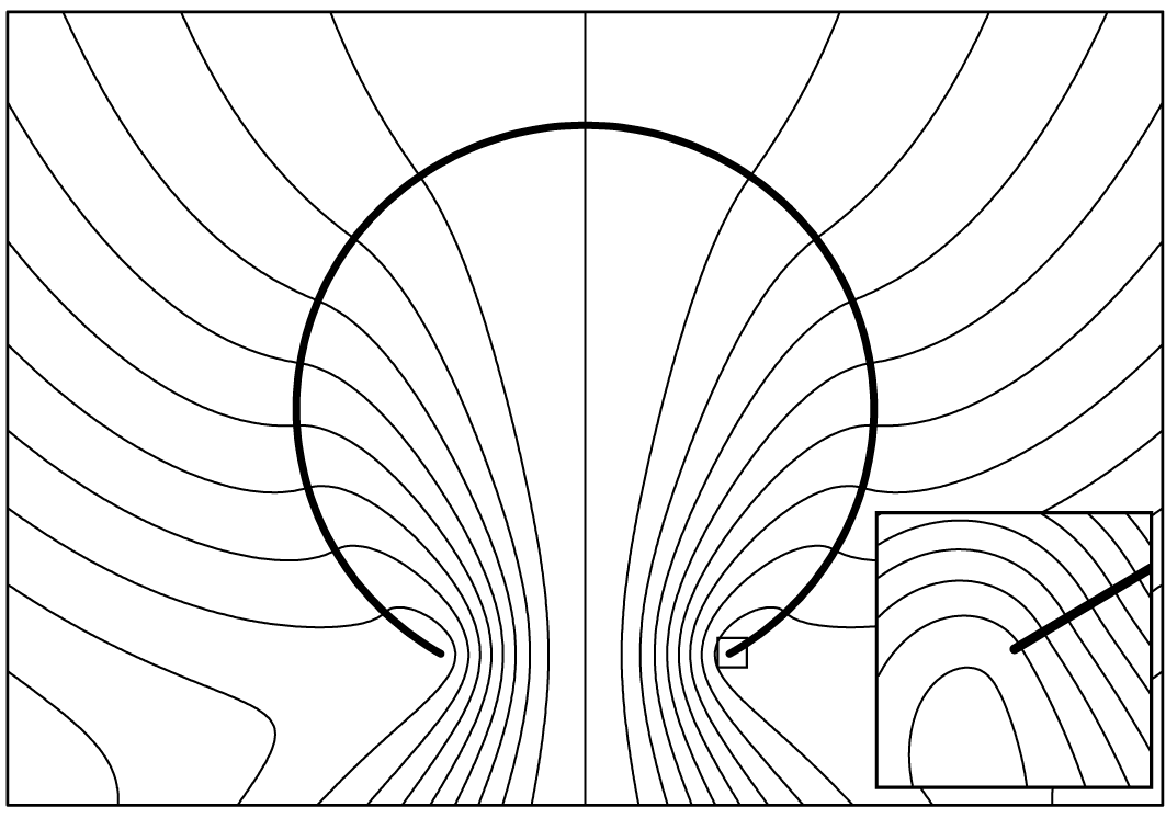
In accord with the boundary condition (4.2), the streamlines of the closed-form expression (4.31) are everywhere perpendicular to
 $\unicode[STIX]{x1D6F4}.$
Assuming
 $U_{1}$
is negative,
 $\unicode[STIX]{x1D6F4}$
moves towards the origin as if in a sink flow while streamlines point outward through the hole opening. Even though
 $\unicode[STIX]{x1D6F4}$
and the efflux move in apparently opposite directions, the velocity is continuous at the edge of the surface (inset, diameter one thousandth that of the sphere, (4.36) and (4.37)).

I have numerically compared (4.31) against the series (4.22) and the two representations are in agreement everywhere. Figure 6 plots the streamlines generated from (4.31). Sending
 $r\rightarrow 1$
in (4.31) gives
 $$\begin{eqnarray}\unicode[STIX]{x1D713}(1,\unicode[STIX]{x1D703})=\left\{\begin{array}{@{}ll@{}}\displaystyle \cos \unicode[STIX]{x1D703}-1, & 0\leqslant \unicode[STIX]{x1D703}\leqslant \unicode[STIX]{x1D6FC},\\ \displaystyle (\cos \unicode[STIX]{x1D703}-1)\left[1-\frac{2}{\unicode[STIX]{x03C0}}\operatorname{atan}\left(\frac{\unicode[STIX]{x1D708}}{2\sin (\unicode[STIX]{x1D6FC}/2)}\right)\right] & \\ \displaystyle \quad +\,\frac{4}{3}D\unicode[STIX]{x1D708}^{3}-2\unicode[STIX]{x03C0}^{-1}\sin \left(\frac{\unicode[STIX]{x1D6FC}}{2}\right)\unicode[STIX]{x1D708}, & \unicode[STIX]{x1D6FC}<\unicode[STIX]{x1D703}\leqslant \unicode[STIX]{x03C0},\end{array}\right.\end{eqnarray}$$
and
 $$\begin{eqnarray}\frac{\unicode[STIX]{x2202}\unicode[STIX]{x1D713}}{\unicode[STIX]{x2202}r}(1,\unicode[STIX]{x1D703})=\left\{\begin{array}{@{}ll@{}}\displaystyle 0, & 0\leqslant \unicode[STIX]{x1D703}\leqslant \unicode[STIX]{x1D6FC},\\ \displaystyle -4D(1+\cos \unicode[STIX]{x1D703})\unicode[STIX]{x1D708}, & \unicode[STIX]{x1D6FC}<\unicode[STIX]{x1D703}\leqslant \unicode[STIX]{x03C0},\end{array}\right.\end{eqnarray}$$
where
 $\unicode[STIX]{x1D708}=\sqrt{2(\cos \unicode[STIX]{x1D6FC}-\cos \unicode[STIX]{x1D703})}.$
Comparing (4.36), (4.37) to (4.4) on
 $[0,\unicode[STIX]{x1D6FC}]$
furnishes the analytical validation of formula (4.31). These piecewise expressions also supply the mixed boundary values that were absent on
 $(\unicode[STIX]{x1D6FC},\unicode[STIX]{x03C0}],$
the open part of the sphere. The functions
 $\unicode[STIX]{x2202}_{\unicode[STIX]{x1D703}}\unicode[STIX]{x1D713}(1,\unicode[STIX]{x1D703})$
and
 $\unicode[STIX]{x2202}_{r}\unicode[STIX]{x1D713}(1,\unicode[STIX]{x1D703})$
are continuous along
 $[0,\unicode[STIX]{x03C0}],$
showing that the velocity components
 $u_{r}$
and
 $u_{\unicode[STIX]{x1D703}}$
are everywhere continuous (figure 6, inset). They behave as the square root in the distance to the edge of the hole (Moffatt Reference Moffatt1964).
5 Vorticity and pressure
This section introduces a change of basis formula that enables the analytic expression of the pressure without further complication. The procedure begins by applying the Stokes operator to (4.31):
 $$\begin{eqnarray}E^{2}\unicode[STIX]{x1D713}=\text{Im}\left\{\begin{array}{@{}ll@{}}\displaystyle 3\unicode[STIX]{x03C0}^{-1}k_{2}+\text{i}(C-4B)k_{3/2}+(1+\text{e}^{-\text{i}\unicode[STIX]{x1D6FC}})(\unicode[STIX]{x03C0}^{-1}-4\text{i}\text{e}^{+\text{i}\unicode[STIX]{x1D6FC}/2}D)g, & r<1,\\ \displaystyle -3\unicode[STIX]{x03C0}^{-1}k_{1}+\text{i}(C-4B)k_{3/2}+(1+\text{e}^{-\text{i}\unicode[STIX]{x1D6FC}})(\unicode[STIX]{x03C0}^{-1}+4\text{i}\text{e}^{-\text{i}\unicode[STIX]{x1D6FC}/2}D)g, & r>1.\end{array}\right.\end{eqnarray}$$
In accord with the Stokes equation
 $E^{4}\unicode[STIX]{x1D713}=0,$
the dimensionless vorticity
 $E^{2}\unicode[STIX]{x1D713}$
is a linear combination of solutions to the Stokes operator equation;
 $E^{2}g=E^{2}k_{m}=0.$
This motivates the following definitions. For
 $-1\leqslant x\leqslant 1,$
 $|\unicode[STIX]{x1D701}|<1$
and
 $r<1,$
let
 $$\begin{eqnarray}\displaystyle & \displaystyle h(\unicode[STIX]{x1D701},x)=\frac{1}{\sqrt{1-2x\unicode[STIX]{x1D701}+\unicode[STIX]{x1D701}^{2}}}-1=\mathop{\sum }_{n=1}^{\infty }\unicode[STIX]{x1D701}^{n}P_{n}(x), & \displaystyle\end{eqnarray}$$
 $$\begin{eqnarray}\displaystyle & \displaystyle l_{m}(r,\unicode[STIX]{x1D703})=r^{m-1}\int _{0}^{r\text{e}^{\text{i}\unicode[STIX]{x1D6FC}}}h(\unicode[STIX]{x1D709},\cos \unicode[STIX]{x1D703})\frac{\text{d}\unicode[STIX]{x1D709}}{\unicode[STIX]{x1D709}^{m}}=\mathop{\sum }_{n=1}^{\infty }\frac{\text{e}^{\text{i}(n-m+1)\unicode[STIX]{x1D6FC}}}{n-m+1}r^{n}P_{n}(\cos \unicode[STIX]{x1D703}), & \displaystyle\end{eqnarray}$$
 $$\begin{eqnarray}\displaystyle l_{m_{1},m_{2}}(r,\unicode[STIX]{x1D703}) & = & \displaystyle r^{m_{1}+m_{2}-2}\int _{0}^{r\text{e}^{\text{i}\unicode[STIX]{x1D6FC}}}\int _{0}^{\unicode[STIX]{x1D709}_{2}}h(\unicode[STIX]{x1D709}_{1},\cos \unicode[STIX]{x1D703})\frac{\text{d}\unicode[STIX]{x1D709}_{1}}{\unicode[STIX]{x1D709}_{1}^{m_{1}}}\frac{\text{d}\unicode[STIX]{x1D709}_{2}}{\unicode[STIX]{x1D709}_{2}^{m_{2}}}\nonumber\\ \displaystyle & = & \displaystyle \mathop{\sum }_{n=1}^{\infty }\frac{\text{e}^{\text{i}(n-m_{1}-m_{2}+2)\unicode[STIX]{x1D6FC}}}{(n-m_{1}+1)(n-m_{1}-m_{2}+2)}r^{n}P_{n}(\cos \unicode[STIX]{x1D703}).\end{eqnarray}$$
Like the pressure
 $p$
in the Stokes equations, the functions
 $h,$
 $l_{m}$
and
 $l_{m_{1},m_{2}}$
are harmonic. The reflection method,
 $$\begin{eqnarray}f(r,\unicode[STIX]{x1D703})=r^{-1}f(r^{-1},\unicode[STIX]{x1D703}),\quad 0<r<\infty ,\end{eqnarray}$$
applied to
 $f(r,\unicode[STIX]{x1D703})=h(r\text{e}^{\text{i}\unicode[STIX]{x1D6FC}},\cos \unicode[STIX]{x1D703}),$
 $l_{m}(r,\unicode[STIX]{x1D703}),$
 $l_{m_{1},m_{2}}(r,\unicode[STIX]{x1D703})$
gives the appropriate harmonic extension to the values (5.2), (5.3) and (5.4) for
 $r>1.$
The selection of the coefficients in (5.3) and (5.4), as made evident shortly, stems from the way the coefficients of (4.26) and (4.27) transform under the vorticity to pressure map.
The dimensionless pressure
 $\tilde{p}$
comes from the vorticity
 $E^{2}\unicode[STIX]{x1D713}$
by way of the formula
 $$\begin{eqnarray}\frac{1}{r^{2}\sin \unicode[STIX]{x1D703}}\frac{\unicode[STIX]{x2202}E^{2}\unicode[STIX]{x1D713}}{\unicode[STIX]{x2202}\unicode[STIX]{x1D703}}=-\frac{\unicode[STIX]{x2202}\tilde{p}}{\unicode[STIX]{x2202}r}.\end{eqnarray}$$
Applying (5.6) to the series (4.26) and (4.27) gives
 $$\begin{eqnarray}\frac{1}{r^{2}\sin \unicode[STIX]{x1D703}}\frac{\unicode[STIX]{x2202}g}{\unicode[STIX]{x2202}\unicode[STIX]{x1D703}}=\frac{\unicode[STIX]{x2202}}{\unicode[STIX]{x2202}r}\left\{\begin{array}{@{}l@{}}\displaystyle 2\text{e}^{\text{i}\unicode[STIX]{x1D6FC}}h+\text{e}^{\text{i}\unicode[STIX]{x1D6FC}}l_{1},\\ \displaystyle -2\text{e}^{\text{i}\unicode[STIX]{x1D6FC}}h+l_{0},\end{array}\right.\quad \frac{1}{r^{2}\sin \unicode[STIX]{x1D703}}\frac{\unicode[STIX]{x2202}k_{m}}{\unicode[STIX]{x2202}\unicode[STIX]{x1D703}}=\frac{\unicode[STIX]{x2202}}{\unicode[STIX]{x2202}r}\left\{\begin{array}{@{}l@{}}\displaystyle 2l_{m-1}+l_{1,m-1},\\ \displaystyle -2l_{m-1}+l_{0,m}.\end{array}\right.\end{eqnarray}$$
The piecewise definitions are for the conditions
 $r<1$
and
 $r>1,$
respectively. The identities in (5.7) follow from the relation
 ${\mathcal{Q}}_{n}^{\prime }(x)=-(2n+1)P_{n}(x).$
To deal with the term
 $k_{3/2},$
there are also the helpful simplifications
 $$\begin{eqnarray}2l_{1/2}+l_{1,1/2}=2\text{e}^{\text{i}\unicode[STIX]{x1D6FC}/2}l_{1},\quad -2l_{1/2}+l_{0,3/2}=-2\text{e}^{-\text{i}\unicode[STIX]{x1D6FC}/2}l_{0},\end{eqnarray}$$
coming from term-wise comparison of the series (5.3) and (5.4).
Applying (5.6), (5.7) and (5.8) to (5.1) furnishes the analytical expression for the dimensionless pressure:
 $$\begin{eqnarray}\displaystyle \tilde{p} & = & \displaystyle \int \frac{\unicode[STIX]{x2202}\tilde{p}}{\unicode[STIX]{x2202}r}\,\text{d}r=-\int \frac{1}{r^{2}\sin \unicode[STIX]{x1D703}}\frac{\unicode[STIX]{x2202}E^{2}\unicode[STIX]{x1D713}}{\unicode[STIX]{x2202}\unicode[STIX]{x1D703}}\text{d}r\nonumber\\ \displaystyle & = & \displaystyle \left\{\begin{array}{@{}l@{}}\displaystyle \tilde{p}_{0}-\text{Im}[\!3\unicode[STIX]{x03C0}^{-1}(2l_{1}+l_{1,1})+2\text{i}(C-4B)\text{e}^{+\text{i}\unicode[STIX]{x1D6FC}/2}l_{1}\\ \displaystyle \quad +\,(1+\text{e}^{-\text{i}\unicode[STIX]{x1D6FC}})(\unicode[STIX]{x03C0}^{-1}-4\text{i}\text{e}^{+\text{i}\unicode[STIX]{x1D6FC}/2}D)(2\text{e}^{\text{i}\unicode[STIX]{x1D6FC}}h+\text{e}^{\text{i}\unicode[STIX]{x1D6FC}}l_{1})\!],\quad r<1,\\ \displaystyle \tilde{p}_{\infty }-\text{Im}[3\unicode[STIX]{x03C0}^{-1}(2l_{0}-l_{0,1})-2\text{i}(C-4B)\text{e}^{-\text{i}\unicode[STIX]{x1D6FC}/2}l_{0}\\ \displaystyle \quad -\,(1+\text{e}^{-\text{i}\unicode[STIX]{x1D6FC}})(\unicode[STIX]{x03C0}^{-1}+4\text{i}\text{e}^{-\text{i}\unicode[STIX]{x1D6FC}/2}D)(2\text{e}^{\text{i}\unicode[STIX]{x1D6FC}}h-l_{0})],\quad r>1.\end{array}\right.\end{eqnarray}$$
The scalar parameters
 $\tilde{p}_{0}$
and
 $\tilde{p}_{\infty }$
are constants of integration. The constant
 $\tilde{p}_{0}$
is the internal pressure evaluated at the origin and
 $\tilde{p}_{\infty }$
is the ambient reference pressure. They satisfy the matching condition
 $$\begin{eqnarray}\lim _{r\rightarrow 1^{-}}\tilde{p}(r,\unicode[STIX]{x03C0})-\lim _{r\rightarrow 1^{+}}\tilde{p}(r,\unicode[STIX]{x03C0})=0,\end{eqnarray}$$
since
 $\tilde{p}(r,\unicode[STIX]{x1D703})$
is continuous at
 $r=1$
for any
 $\unicode[STIX]{x1D703}\in (\unicode[STIX]{x1D6FC},\unicode[STIX]{x03C0}].$
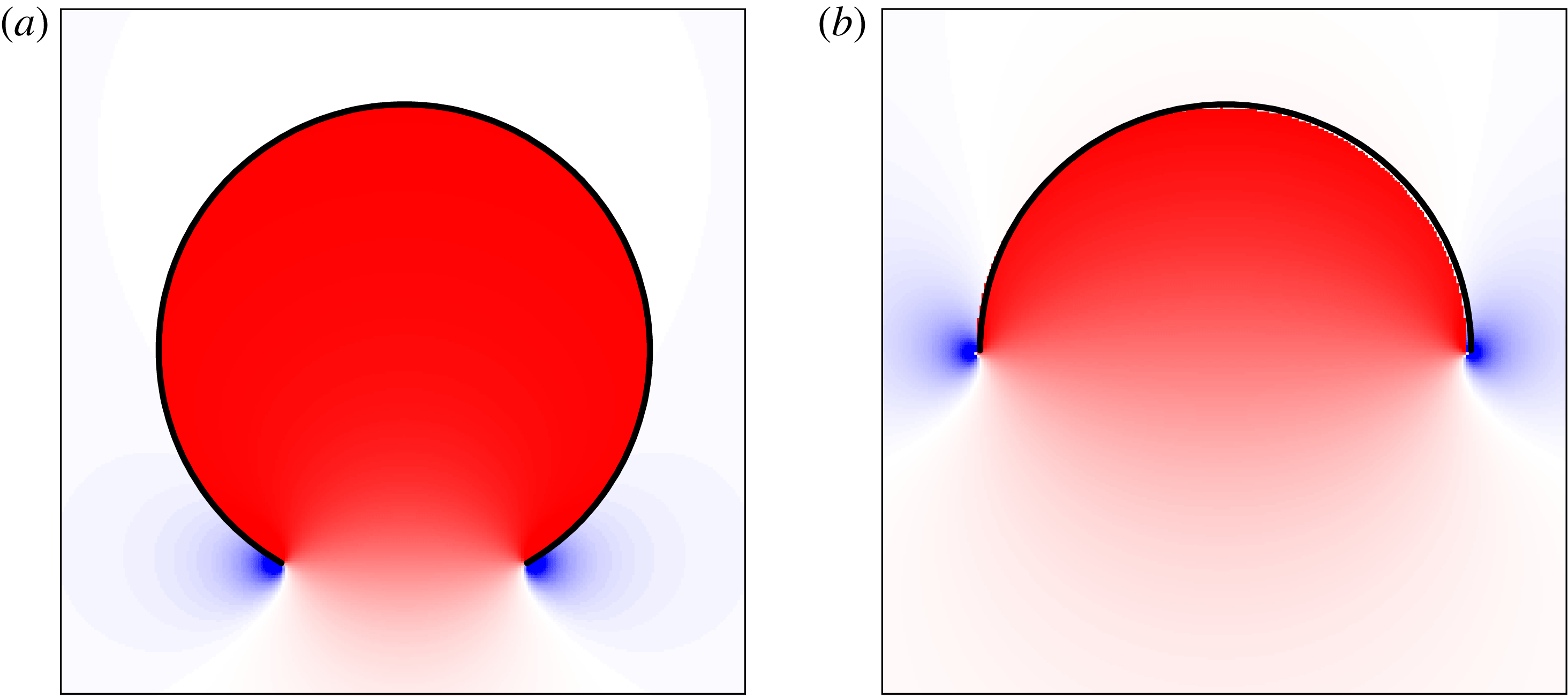
Figure 7 shows how the piecewise definition of pressure is smooth across the hole opening.
To evaluate the limit (5.10), set
 $r=1$
and
 $\unicode[STIX]{x1D703}=\unicode[STIX]{x03C0}$
in (5.2), (5.3) and (5.4). This gives the Taylor series
 $$\begin{eqnarray}\displaystyle h(\unicode[STIX]{x1D701},-1)=\frac{-\unicode[STIX]{x1D701}}{1+\unicode[STIX]{x1D701}},\quad l_{0}(1,\unicode[STIX]{x03C0})=\log (1+\unicode[STIX]{x1D701})-\unicode[STIX]{x1D701},\quad l_{1}(1,\unicode[STIX]{x03C0})=-\text{log}\,(1+\unicode[STIX]{x1D701}),\quad \qquad & & \displaystyle\end{eqnarray}$$
 $$\begin{eqnarray}\displaystyle l_{0,1}(1,\unicode[STIX]{x03C0})=-\unicode[STIX]{x1D701}-\operatorname{Li}_{2}(-\unicode[STIX]{x1D701}),\quad l_{1,1}(1,\unicode[STIX]{x03C0})=\operatorname{Li}_{2}(-\unicode[STIX]{x1D701}), & & \displaystyle\end{eqnarray}$$
where
 $\unicode[STIX]{x1D701}=\text{e}^{\text{i}\unicode[STIX]{x1D6FC}}$
and where
 $\operatorname{Li}_{2}(\unicode[STIX]{x1D709})=\sum _{n=1}^{\infty }\unicode[STIX]{x1D709}^{n}/n^{2}$
is Spence’s dilogarithm function (Zagier Reference Zagier2007). Making the appropriate substitutions into the matching condition (5.10) yields the dimensionless pressure jump:
 $$\begin{eqnarray}\displaystyle \unicode[STIX]{x0394}\tilde{p}=\tilde{p}_{0}-\tilde{p}_{\infty } & = & \displaystyle \frac{2(\cos \unicode[STIX]{x1D6FC}-1)}{\unicode[STIX]{x03C0}\sin ^{3}\unicode[STIX]{x1D6FC}}\left[(1-2\cos \unicode[STIX]{x1D6FC})\sin ^{2}\unicode[STIX]{x1D6FC}+\frac{1}{2}\unicode[STIX]{x1D6FC}(11-\cos \unicode[STIX]{x1D6FC})\sin \unicode[STIX]{x1D6FC}\right.\nonumber\\ \displaystyle & & \displaystyle +\left.3\unicode[STIX]{x1D6FC}^{2}(2+\cos \unicode[STIX]{x1D6FC})\sin ^{2}\frac{\unicode[STIX]{x1D6FC}}{2}\right].\end{eqnarray}$$
In accord with the dilation implied by (4.4),
 $\unicode[STIX]{x0394}\tilde{p}$
is negative for all
 $0<\unicode[STIX]{x1D6FC}<\unicode[STIX]{x03C0}.$
The dilogarithm terms cancel in the subtraction (5.10) and do not enter (5.13).
The pressure maps derive from the expressions (5.9) and (5.14). White represents a zero ambient reference pressure and red coloration is for a positive internal pressure. Blue colouration shows the negative inverse square root singularity just outside the edge of the hole. (a) For a small hole,
 $p$
behaves like the Laplace pressure of an intact sphere, with internal values almost everywhere equal to
 $\unicode[STIX]{x0394}p.$
(b) For a larger hole, the pressure gradients are more diffuse than in panel (a).

The measured and dimensionless pressures
 $p$
and
 $\tilde{p},$
respectively, satisfy
 $$\begin{eqnarray}p(r,\unicode[STIX]{x1D703})=\frac{\unicode[STIX]{x1D707}U_{1}}{R}\tilde{p}\left(\frac{r}{R},\unicode[STIX]{x1D703}\right).\end{eqnarray}$$
Let
 $q$
be the volumetric flow rate. Volume conservation sets the radial velocity
 $U_{1}$
as a function of
 $q$
according to (2.7). Using the change of variables (5.14) gives
 $$\begin{eqnarray}\unicode[STIX]{x0394}p=\frac{\unicode[STIX]{x1D707}U_{1}}{R}\unicode[STIX]{x0394}\tilde{p}=\frac{\unicode[STIX]{x0394}\tilde{p}\sin ^{3}\unicode[STIX]{x1D6FC}}{2\unicode[STIX]{x03C0}(\cos \unicode[STIX]{x1D6FC}-1)}\frac{\unicode[STIX]{x1D707}q}{c^{3}},\end{eqnarray}$$
where
 $c=R\sin \unicode[STIX]{x1D6FC}$
is the radius of the hole opening. This supplies the derivation of the identity (3.2) for
 $\unicode[STIX]{x0394}p^{(1)}.$
Let
 ${\mathcal{K}}=\unicode[STIX]{x0394}\tilde{p}\sin ^{3}(\unicode[STIX]{x1D6FC})/[2\unicode[STIX]{x03C0}(\cos \unicode[STIX]{x1D6FC}-1)]$
be the dimensionless factor in (5.15). Recall from the Taylor series (3.3) that
 ${\mathcal{K}}$
equals
 $3$
to second order at
 $\unicode[STIX]{x1D6FC}=\unicode[STIX]{x03C0}.$
Perhaps surprisingly, the absolute maximum
 ${\mathcal{K}}\approx 3.0613,$
attained at
 $\unicode[STIX]{x1D6FC}\approx 2.6544$
radians, is slightly larger than the value
 $3$
attained at
 $\unicode[STIX]{x1D6FC}=\unicode[STIX]{x03C0}.$
To derive the identities (3.4) and (3.5) for the pressure jumps
 $\unicode[STIX]{x0394}p^{(2)}$
and
 $\unicode[STIX]{x0394}p^{(3)},$
respectively, I applied the methods of the present section to the motions
 $(\boldsymbol{u}^{(2)},p^{(2)})$
and
 $(\boldsymbol{u}^{(3)},p^{(3)})$
from previous works. An alternative, perhaps more straightforward derivation of (3.5) uses (4.23) to record the value of the coefficient
 $F_{31},$
the reciprocal identity
 $F_{13}=F_{31}$
and finally (3.13) to get
 $\unicode[STIX]{x0394}p^{(3)}=-\unicode[STIX]{x1D707}F_{13}U_{3}/(4\unicode[STIX]{x03C0}R).$
I numerically verified (5.9) and (5.13) against the infinite series for
 $\tilde{p}$
derived directly from (4.22). To evaluate (5.9) at other points in the aqueous region,
 $$\begin{eqnarray}l_{0}(r,\unicode[STIX]{x1D703})=r^{-1}\left[\log \left(\frac{\unicode[STIX]{x1D701}-x+s}{1-x}\right)-\unicode[STIX]{x1D701}\right],\quad l_{1}(r,\unicode[STIX]{x1D703})=-\text{log}\left(\frac{1-\unicode[STIX]{x1D701}x+s}{2}\right),\end{eqnarray}$$
for
 $r<1,$
where
 $\unicode[STIX]{x1D701}=r\text{e}^{\text{i}\unicode[STIX]{x1D6FC}},$
 $x=\cos \unicode[STIX]{x1D703}$
and
 $s=\sqrt{1-2x\unicode[STIX]{x1D701}+\unicode[STIX]{x1D701}^{2}}.$
The functions
 $l_{0,1}$
and
 $l_{1,1}$
do not admit an expression in terms of elementary functions. Their series (5.4), however, converge quadratically and so truncation is an efficient way to estimate their sum.
6 A theorem concerning the dissipation function
Energy dissipation for the contracting spherical cap is a special case that generalizes to arbitrary piecewise smooth, bounded surfaces
 $\unicode[STIX]{x1D6E4}.$
Like the spherical cap, the surface
 $\unicode[STIX]{x1D6E4}$
is an internal boundary, meaning that every surface element makes contact with the aqueous region on two sides. The main identity (6.9) of this section quantifies the rate of work performed by the surface contracting in the fluid.
Consider any solution
 $(\boldsymbol{u},p)$
to the creeping motion equations that takes boundary values on
 $\unicode[STIX]{x1D6E4}$
continuously and has bounded pressure. Assume that
 $\boldsymbol{x}_{0}\notin \unicode[STIX]{x1D6E4}$
and let
 $\boldsymbol{u}^{\ast }$
be the sink or source flow (Happel & Brenner Reference Happel and Brenner1965, p. 107)
 $$\begin{eqnarray}\boldsymbol{u}^{\ast }=\frac{q^{\ast }}{4\unicode[STIX]{x03C0}r^{2}}\boldsymbol{i}_{r}\quad \text{in }\mathbb{R}^{3}\setminus \{\boldsymbol{x}_{0}\},\end{eqnarray}$$
with
 $r=|\boldsymbol{x}-\boldsymbol{x}_{0}|.$
Select
 $a>0$
sufficiently small so that the intersection of
 $\unicode[STIX]{x1D6E4}$
with
 $\{r<a\}$
is empty and
 $b_{0}<\infty$
sufficiently large so that
 $\unicode[STIX]{x1D6E4}$
is contained in the ball
 $\{r<b_{0}\}.$
Let
 $b>b_{0}.$
Employing the reciprocal identity of Lorentz,
 $$\begin{eqnarray}\displaystyle 0 & = & \displaystyle \int _{\{a<r<b\}}\operatorname{div}(\boldsymbol{u}^{\ast }\boldsymbol{\cdot }\unicode[STIX]{x1D64F}-\boldsymbol{u}\boldsymbol{\cdot }\unicode[STIX]{x1D64F}^{\ast })\,\text{d}x\nonumber\\ \displaystyle & = & \displaystyle \int _{\{r=b\}}(\boldsymbol{u}^{\ast }\boldsymbol{\cdot }\unicode[STIX]{x1D64F}-\boldsymbol{u}\boldsymbol{\cdot }\unicode[STIX]{x1D64F}^{\ast })\boldsymbol{\cdot }\boldsymbol{i}_{r}\,\text{d}A-\int _{\{r=a\}}(\boldsymbol{u}^{\ast }\boldsymbol{\cdot }\unicode[STIX]{x1D64F}-\boldsymbol{u}\boldsymbol{\cdot }\unicode[STIX]{x1D64F}^{\ast })\boldsymbol{\cdot }\boldsymbol{i}_{r}\,\text{d}A\nonumber\\ \displaystyle & & \displaystyle +\,\int _{\unicode[STIX]{x1D6E4}}[(\boldsymbol{u}^{\ast }\boldsymbol{\cdot }\unicode[STIX]{x1D64F}-\boldsymbol{u}\boldsymbol{\cdot }\unicode[STIX]{x1D64F}^{\ast })\boldsymbol{\cdot }\text{d}\boldsymbol{S}]_{\pm }=I_{1}+I_{2}+I_{3}.\end{eqnarray}$$
Here
 $$\begin{eqnarray}\unicode[STIX]{x1D64F}^{\ast }=\frac{\unicode[STIX]{x1D707}q^{\ast }}{2\unicode[STIX]{x03C0}r^{3}}(\boldsymbol{I}-3\boldsymbol{i}_{r}\boldsymbol{i}_{r}),\quad \unicode[STIX]{x1D64F}=-\boldsymbol{I}p+2\unicode[STIX]{x1D707}\unicode[STIX]{x1D750},\end{eqnarray}$$
are dyadic stress tensors for
 $\boldsymbol{u}^{\ast }$
and
 $\boldsymbol{u},$
respectively. The symbol
 $[(\;\;)\boldsymbol{\cdot }\text{d}\boldsymbol{S}]_{\pm }$
denotes the net rate of work done by the two sides of the surface element.
The application of the divergence theorem in (6.2) is justified because the singularity of
 $\boldsymbol{u}^{\ast }$
and
 $\unicode[STIX]{x1D64F}^{\ast }$
lies outside the domain of integration. Also,
 $\boldsymbol{u}$
is everywhere continuous; the singularities of the stress
 $\unicode[STIX]{x1D64F}$
are summable and
 $O(\unicode[STIX]{x1D70C}^{-1/2})$
in the distance
 $\unicode[STIX]{x1D70C}$
to any edges or corners (Moffatt Reference Moffatt1964).
By the divergence theorem and the identities
 $\operatorname{div}((\boldsymbol{x}-\boldsymbol{x}_{0})\boldsymbol{\cdot }\unicode[STIX]{x1D64F})=-3p$
and
 $\operatorname{div}\boldsymbol{u}=0,$
 $$\begin{eqnarray}\displaystyle I_{2} & = & \displaystyle -\frac{q^{\ast }}{4\unicode[STIX]{x03C0}a^{3}}\int _{\{r=a\}}[(\boldsymbol{x}-\boldsymbol{x}_{0})\boldsymbol{\cdot }\unicode[STIX]{x1D64F}+4\unicode[STIX]{x1D707}\boldsymbol{u}]\boldsymbol{\cdot }\boldsymbol{i}_{r}\,\text{d}A\nonumber\\ \displaystyle & = & \displaystyle -\frac{q^{\ast }}{4\unicode[STIX]{x03C0}a^{3}}\int _{\{r<a\}}\operatorname{div}((\boldsymbol{x}-\boldsymbol{x}_{0})\boldsymbol{\cdot }\unicode[STIX]{x1D64F})+4\unicode[STIX]{x1D707}\operatorname{div}\boldsymbol{u}\,\text{d}x=\frac{3q^{\ast }}{4\unicode[STIX]{x03C0}a^{3}}\int _{\{r<a\}}p\,\text{d}x.\end{eqnarray}$$
Applying the mean value identity to the last integral gives
 $$\begin{eqnarray}I_{2}=q^{\ast }p(\boldsymbol{x}_{0}).\end{eqnarray}$$
Any bounded harmonic function
 $p$
on the exterior domain
 $\{r>b_{0}\}$
has a well-defined limit
 $p_{\infty }$
at infinity. In three space dimensions (Dancer, Daners & Hauer Reference Dancer, Daners and Hauer2015), there is a constant
 $C_{0}$
for which
 $$\begin{eqnarray}|p-p_{\infty }|\leqslant C_{0}r^{-1},\quad \text{for all }r>b_{0}.\end{eqnarray}$$
Using
 $\operatorname{div}((\boldsymbol{x}-\boldsymbol{x}_{0})\boldsymbol{\cdot }\unicode[STIX]{x1D64F})=-3p$
and
 $\operatorname{div}\boldsymbol{u}=0$
to integrate over
 $\{b_{0}<r<b\},$
 $$\begin{eqnarray}\displaystyle I_{1} & = & \displaystyle \frac{q^{\ast }}{4\unicode[STIX]{x03C0}b^{3}}\left(\int _{\{r=b_{0}\}}[(\boldsymbol{x}-\boldsymbol{x}_{0})\boldsymbol{\cdot }\unicode[STIX]{x1D64F}+4\unicode[STIX]{x1D707}\boldsymbol{u}]\boldsymbol{\cdot }\boldsymbol{i}_{r}\,\text{d}A-3\int _{b_{0}<r<b}p\,\text{d}x\right)\nonumber\\ \displaystyle & = & \displaystyle \frac{q^{\ast }}{4\unicode[STIX]{x03C0}b^{3}}\left(\int _{\{r=b_{0}\}}[(\boldsymbol{x}-\boldsymbol{x}_{0})\boldsymbol{\cdot }\unicode[STIX]{x1D64F}+4\unicode[STIX]{x1D707}\boldsymbol{u}]\boldsymbol{\cdot }\boldsymbol{i}_{r}\,\text{d}A-3\int _{b_{0}<r<b}p-p_{\infty }\,\text{d}x\right)\nonumber\\ \displaystyle & & \displaystyle -\,q^{\ast }p_{\infty }\left(1-\frac{b_{0}^{3}}{b^{3}}\right)=-q^{\ast }p_{\infty }+O(b^{-1}).\end{eqnarray}$$
This implies that
 $\lim _{b\rightarrow \infty }I_{1}=-q^{\ast }p_{\infty }.$
But
 $I_{1}+I_{2}+I_{3}=0$
with
 $I_{2}$
and
 $I_{3}$
independent of
 $b.$
It follows that
 $$\begin{eqnarray}I_{1}=-q^{\ast }p_{\infty }.\end{eqnarray}$$
In the integral
 $I_{3},$
 $[\boldsymbol{u}\boldsymbol{\cdot }\unicode[STIX]{x1D64F}^{\ast }\boldsymbol{\cdot }\text{d}\boldsymbol{S}]_{\pm }=0$
since the fields
 $\boldsymbol{u}$
and
 $\unicode[STIX]{x1D64F}^{\ast }$
attain values on
 $\unicode[STIX]{x1D6E4}$
continuously. Using (6.2), (6.8) and (6.5) yields
 $$\begin{eqnarray}\int _{\unicode[STIX]{x1D6E4}}[\boldsymbol{u}^{\ast }\boldsymbol{\cdot }\unicode[STIX]{x1D64F}\boldsymbol{\cdot }\text{d}\boldsymbol{S}]_{\pm }=-q^{\ast }\unicode[STIX]{x0394}p_{L},\end{eqnarray}$$
where
 $\unicode[STIX]{x0394}p_{L}=p(\boldsymbol{x}_{0})-\lim _{\boldsymbol{x}\rightarrow \infty }p(\boldsymbol{x}).$
The interpretation of (6.9) is that the rate of work transmitted by a surface onto a sink/source flow, regardless of the prevailing boundary conditions, is the same as the strength of sink/source times the negative jump in pressure.
6.1 Derivation of the radial resistance coefficients
As an application of (6.9), consider the special case
 $$\begin{eqnarray}\unicode[STIX]{x1D6E4}=\unicode[STIX]{x1D6F4},\quad q^{\ast }=4\unicode[STIX]{x03C0}R^{2}U_{1}.\end{eqnarray}$$
Take the motion
 $(\boldsymbol{u},p)$
to be the superposition solution (2.9). Then
 $\boldsymbol{u}^{\ast }=\boldsymbol{u}^{(1)}$
on
 $\unicode[STIX]{x1D6F4}.$
It follows from (3.6) and (6.9) that
 $$\begin{eqnarray}\displaystyle F_{1}U_{1} & = & \displaystyle \unicode[STIX]{x1D707}RU_{1}(F_{11}U_{1}+F_{12}U_{2}+F_{13}U_{3})\nonumber\\ \displaystyle & = & \displaystyle \int _{\unicode[STIX]{x1D6F4}}[\boldsymbol{u}^{(1)}\boldsymbol{\cdot }\unicode[STIX]{x1D64F}\boldsymbol{\cdot }\text{d}\boldsymbol{S}]_{\pm }=\int _{\unicode[STIX]{x1D6F4}}[\boldsymbol{u}^{\ast }\boldsymbol{\cdot }\unicode[STIX]{x1D64F}\boldsymbol{\cdot }\text{d}\boldsymbol{S}]_{\pm }=-4\unicode[STIX]{x03C0}R^{2}U_{1}\unicode[STIX]{x0394}p_{L}\nonumber\\ \displaystyle & = & \displaystyle -4\unicode[STIX]{x03C0}R^{2}U_{1}(\unicode[STIX]{x0394}p^{(1)}+\unicode[STIX]{x0394}p^{(2)}+\unicode[STIX]{x0394}p^{(3)}).\end{eqnarray}$$
Dividing through by
 $U_{1}$
furnishes the derivation of the identity (3.14) for
 $F_{1}.$
To evaluate the radial resistance coefficients
 $F_{1i},$
note that the jumps in pressure
 $\unicode[STIX]{x0394}p^{(i)}$
are proportional to
 $U_{i},$
 $i=1,2,3,$
respectively. Thus
 $$\begin{eqnarray}F_{1i}=\frac{-4\unicode[STIX]{x03C0}R\unicode[STIX]{x0394}p^{(i)}}{\unicode[STIX]{x1D707}U_{i}},\quad i=1,2,3.\end{eqnarray}$$
The expressions (3.2), (3.4) and (3.5) for
 $\unicode[STIX]{x0394}p^{(i)}$
then furnish the desired values for
 $F_{1i}.$
To compare (6.9) to other well-known results, consider the case
 $U_{2}=U_{3}=0$
so that
 $(\boldsymbol{u},p)=(\boldsymbol{u}^{(1)},p^{(1)}).$
Then
 $\unicode[STIX]{x1D64F}=\unicode[STIX]{x1D64F}^{(1)}$
and
 $\unicode[STIX]{x0394}p_{L}=\unicode[STIX]{x0394}p^{(1)}$
give
 $$\begin{eqnarray}{\mathcal{E}}=\int _{\unicode[STIX]{x1D6F4}}[\boldsymbol{u}^{(1)}\boldsymbol{\cdot }\unicode[STIX]{x1D64F}^{(1)}\boldsymbol{\cdot }\text{d}\boldsymbol{S}]_{\pm }=-4\unicode[STIX]{x03C0}R^{2}U_{1}\unicode[STIX]{x0394}p^{(1)},\end{eqnarray}$$
where
 ${\mathcal{E}}$
is the dissipation function (3.8). Based on the expression (5.15), the dissipation function has the Taylor expansion
 $$\begin{eqnarray}{\mathcal{E}}=16c\unicode[STIX]{x1D707}U_{1}^{2}+{\textstyle \frac{64}{3}}c\unicode[STIX]{x1D707}U_{1}^{2}\unicode[STIX]{x1D6FC}^{2}+O(\unicode[STIX]{x1D6FC}^{4}c\unicode[STIX]{x1D707}U_{1}^{2}),\end{eqnarray}$$
at
 $\unicode[STIX]{x1D6FC}=0.$
For small
 $\unicode[STIX]{x1D6FC},$
the spherical cap resembles a flat circular disk of radius
 $c=R\sin \unicode[STIX]{x1D6FC}.$
The leading-order term in (6.14) correctly predicts the drag force
 $16c\unicode[STIX]{x1D707}U_{1}$
for broadside translation of the disk parallel to the axis of symmetry.
7 Lateral pressures in pore kinetics
In theoretical studies, researchers have often assumed a Sampson flow to characterize the leak-out flow rate and a one-dimensional pore rate equation, effectively a pore in an infinite planar bilayer, to model pore growth and shrinkage in a liposome. But to account for the spherical geometry and aqueous interactions, consider the dynamical equations (3.9). Pore widening and surface stretching store the energy
 $$\begin{eqnarray}W=2\unicode[STIX]{x03C0}\unicode[STIX]{x1D6FE}c+{\textstyle \frac{1}{2}}K_{A}A_{0}(A/A_{0}-1)^{2},\end{eqnarray}$$
with edge tension
 $\unicode[STIX]{x1D6FE},$
hole radius
 $c=R\sin \unicode[STIX]{x1D6FC},$
area modulus
 $K_{A},$
surface area
 $A=2\unicode[STIX]{x03C0}R^{2}(1-\cos \unicode[STIX]{x1D6FC})$
and area
 $A_{0}=4\unicode[STIX]{x03C0}R_{0}^{2}$
at rest. The pore grows or shrinks depending on whether it is smaller or larger than the critical pore radius set by the available tension (Ilton, DiMaria & Dalnoki-Veress Reference Ilton, Dimaria and Dalnoki-Veress2016). (To prevent
 $c$
from becoming non-positive, the simulations use the modified edge energy
 $2\unicode[STIX]{x03C0}\unicode[STIX]{x1D6FE}c(1+c_{\ast }^{2}/c^{2})$
with
 $c_{\ast }$
equalling the pore radius of minimal edge energy (Poignard, Silve & Wegner Reference Poignard, Silve, Wegner and Damijan2016).)
The internal energy
 $W$
of the spherical cap liposome model is a function of the state variables
 $(R,\unicode[STIX]{x1D6FC},z_{0}),$
and the release of energy sets the surrounding viscous fluid in motion. The kinetic equations (3.9) describing the motion are
 $$\begin{eqnarray}\displaystyle & \displaystyle F_{1}+F_{1}^{\text{s}}=-\unicode[STIX]{x2202}_{R}W=-2\unicode[STIX]{x03C0}\unicode[STIX]{x1D6FE}\sin \unicode[STIX]{x1D6FC}-4\unicode[STIX]{x03C0}\unicode[STIX]{x1D70E}(1-\cos \unicode[STIX]{x1D6FC})R, & \displaystyle\end{eqnarray}$$
 $$\begin{eqnarray}\displaystyle & \displaystyle F_{2}+F_{2}^{\text{s}}=-R^{-1}\unicode[STIX]{x2202}_{\unicode[STIX]{x1D6FC}}W=-2\unicode[STIX]{x03C0}\unicode[STIX]{x1D6FE}\cos \unicode[STIX]{x1D6FC}-2\unicode[STIX]{x03C0}\unicode[STIX]{x1D70E}c, & \displaystyle\end{eqnarray}$$
 $$\begin{eqnarray}\displaystyle & \displaystyle F_{3}+F_{3}^{\text{s}}=-\unicode[STIX]{x2202}_{z_{0}}W=0, & \displaystyle\end{eqnarray}$$
with tension
 $\unicode[STIX]{x1D70E}=K_{A}(A/A_{0}-1).$
The factor
 $R^{-1}$
in (7.3) normalizes the partial derivative in
 $\unicode[STIX]{x1D6FC}.$
The expressions for the aqueous forces
 $F_{i},$
 $i=1,2,3$
use (3.14), (3.15) and (3.16), respectively.
(a) The curves show the numerically integrated time course for (7.2)–(7.4). The model parameters are
 $R(0)=20~\unicode[STIX]{x03BC}\text{m}$
,
 $R_{0}=18~\unicode[STIX]{x03BC}\text{m}$
(horizontal dashed line),
 $K_{A}=2\times 10^{-4}~\text{N}~\text{m}^{-1}$
,
 $c(0)=c_{\ast }=0.05~\unicode[STIX]{x03BC}\text{m}$
,
 $z(0)=0~\unicode[STIX]{x03BC}\text{m}$
,
 $\unicode[STIX]{x1D6FE}=12~\text{pN}$
,
 $\unicode[STIX]{x1D707}=1~\text{mP}~\text{s}$
for distilled water and
 $\unicode[STIX]{x1D707}_{s}=3\times 10^{-9}~\text{Pa}~\text{m}~\text{s}$
(Honerkamp-Smith et al.
Reference Honerkamp-Smith, Woodhouse, Kantsler and Goldstein2013). (b) The curves (i) and (ii) are the transient leak-out volume for (7.2)–(7.4) and (7.6), respectively. The characteristic time of (ii) is shorter in the rapid widening stage and longer in the slow, linear closure stage than for (i). The net efflux at the time of pore collapse for the two models (around 230 ms and 300 ms respectively) is nearly the same, approximately 20 % of initial volume.

In applications, the zero thickness surface
 $\unicode[STIX]{x1D6F4}$
is an idealization of an incompressible fluid layer (e.g. a membrane bilayer) with thickness
 $l\ll R$
and viscosity
 $\unicode[STIX]{x1D707}_{l}.$
The quantities
 $F_{i}^{\text{s}}=(\unicode[STIX]{x2202}_{U_{i}}{\mathcal{E}}_{s})/2$
,
 $i=1,2,3$
are the surface forces for the rate of energy dissipation in
 $\unicode[STIX]{x1D6F4}$
:
 $$\begin{eqnarray}{\mathcal{E}}_{s}=4\unicode[STIX]{x03C0}\unicode[STIX]{x1D707}_{s}[6(1-\cos \unicode[STIX]{x1D6FC})U_{1}^{2}+6\sin \unicode[STIX]{x1D6FC}U_{1}U_{2}+(1+\unicode[STIX]{x1D702}(\unicode[STIX]{x1D6FC}))U_{2}^{2}],\end{eqnarray}$$
with surface viscosity
 $\unicode[STIX]{x1D707}_{s}=l\unicode[STIX]{x1D707}_{l}$
and
 $\unicode[STIX]{x1D702}(\unicode[STIX]{x1D6FC})=2(1+\cos \unicode[STIX]{x1D6FC})[1+2(1-\cos \unicode[STIX]{x1D6FC})^{-1}\log (\cos (\unicode[STIX]{x1D6FC}/2))].$
These expressions agree with previous calculations for the rim-less planar film (Debrégeas, Martin & Brochard-Wyart Reference Debrégeas, Martin and Brochard-Wyart1995) (i.e.
 $F_{2}^{\text{s}}\simeq 4\unicode[STIX]{x03C0}\unicode[STIX]{x1D707}_{s}U_{2}$
at
 $\unicode[STIX]{x1D6FC}=\unicode[STIX]{x03C0}$
).
The derivation of (7.5) assumes the rate of surface dissipation
 $2\unicode[STIX]{x1D707}_{s}\unicode[STIX]{x1D750}_{\unicode[STIX]{x1D6F4}}\boldsymbol{ : }\unicode[STIX]{x1D750}_{\unicode[STIX]{x1D6F4}}+\unicode[STIX]{x1D705}_{s}(\unicode[STIX]{x1D735}_{\unicode[STIX]{x1D6F4}}\boldsymbol{\cdot }\boldsymbol{u})^{2}$
with two-dimensional rate of strain tensor
 $\unicode[STIX]{x1D750}_{\unicode[STIX]{x1D6F4}}$
for the motion (2.4) (Fournier Reference Fournier2015). The bulk viscosity
 $\unicode[STIX]{x1D705}_{s}=2\unicode[STIX]{x1D707}_{s}$
(Leal (Reference Leal2006)) accounts for the change in thickness required to maintain constant volume under (2.5).
Assume a liposome under weak tensions. The membrane surface is not completely smooth but rather has microscopic infoldings that flatten out as the liposome dilates. Thus, the smooth surface
 $\unicode[STIX]{x1D6F4}$
actually represents the projected membrane area and
 $K_{A}=2\times 10^{-4}$
N m
 $^{-1}$
is a suitable area modulus for suppressing infoldings (Fournier & Barbetta Reference Fournier and Barbetta2008; Alam Shibly et al.
Reference Alam Shibly, Ghatak, Sayem Karal, Moniruzzaman and Yamazaki2016). (To clarify, the value of
 $K_{A}$
depends on external factors like strength of illumination. In micropipette aspiration, for example, the taut liposome fluctuates very little and
 $K_{A}$
takes the large value 0.2 N m
 $^{-1}$
for exposing hydrophobic acyl chain to water (Evans & Rawicz Reference Evans and Rawicz1990; Puech & Brochard-Wyart Reference Puech and Brochard-Wyart2004).)
The time course predicted by (7.2)–(7.4) replicates the experimental pattern of pore kinetics (figure 8
a (Brochard-Wyart, de Gennes & Sandre Reference Brochard-Wyart, de Gennes and Sandre2000; Portet & Dimova Reference Portet and Dimova2010)). The simulation starts with a tensed liposome of radius
 $20~\unicode[STIX]{x03BC}\text{m}$
. The radius is
 $18~\unicode[STIX]{x03BC}\text{m}$
in the un-stretched state. This set-up yields an initial tension
 $\unicode[STIX]{x1D70E}=K_{A}(A/A_{0}-1)=4.7\times 10^{-5}~\text{N}~\text{m}^{-1}$
and Young–Laplace pressure
 $2\unicode[STIX]{x1D70E}/R=4.7~\text{Pa}$
sufficient to widen the initially small pore (
 $c=0.05~\unicode[STIX]{x03BC}\text{m}$
at time
 $t=0$
). Both hole widening and spherical contraction can decrease energy. But the resistance to instantaneous changes in
 $\unicode[STIX]{x1D6FC}$
is initially much less than for changes in
 $R,$
and so maximal energy dissipation selects a trajectory where the hole widens first (figure 8
a). Except for very large values of surface viscosity
 $\unicode[STIX]{x1D707}_{s}$
(orders of magnitude larger than
 $3\times 10^{-9}~\text{Pa}~\text{m}~\text{s}$
), it is the aqueous viscosity
 $\unicode[STIX]{x1D707}$
that sets the characteristic time of the trajectories.
Translation is a consequence of momentum conservation (7.4) with
 $F_{3}=0.$
The displacements in the
 $z_{0}$
-variable are appreciable (figure 8
a), and, as far as I am aware, have not been accounted for in any prior theoretical or experimental study of liposome bursting. Moreover, the closed-form solution (2.9) allows for pointwise visualization of the fluid velocity and pressure (supplementary movies 3 and 4), details not easily accessible to microscopy techniques. Figure 11(a), for example, tracks the time taken by individual tracers particles to pass across the hole opening (Singer et al.
Reference Singer, Schuss, Holcman and Eisenberg2006).
It is helpful to compare the Stokes formulation model (7.2)–(7.4) to the classic pore kinetics model (Brochard-Wyart et al. Reference Brochard-Wyart, de Gennes and Sandre2000):
 $$\begin{eqnarray}(2\unicode[STIX]{x03C0}\unicode[STIX]{x1D707}c+2\unicode[STIX]{x1D707}_{s})c^{\prime }=-\unicode[STIX]{x1D6FE}+\unicode[STIX]{x1D70E}c,\quad q=\frac{2\unicode[STIX]{x1D70E}}{R}\frac{c^{3}}{3\unicode[STIX]{x1D707}},\end{eqnarray}$$
with
 $c^{\prime }=\text{d}c/\text{d}t,$
pore radius
 $c=R\sin \unicode[STIX]{x1D6FC},$
tension
 $\unicode[STIX]{x1D70E}=K_{A}(A/A_{0}-1)$
and leak-out flow rate
 $q=-4\unicode[STIX]{x03C0}R^{2}R^{\prime }.$
Note that
 $\cos \unicode[STIX]{x1D6FC}\sim -1$
as
 $\unicode[STIX]{x1D6FC}\rightarrow \unicode[STIX]{x03C0}$
in the right-hand side of (7.3). Although qualitatively similar, there are important distinctions between (7.2)–(7.4) and (7.6).
The classic model ignores translation effects and is thermodynamically inconsistent (Martínez-Balbuena et al.
Reference Martínez-Balbuena, Hernández-Zapata and Santamaría-Holek2015). Actually, (7.6) is a limiting case that takes all reciprocal terms in (7.2)–(7.4) to be zero. For example, the derivation of (7.6b
) assumes that Laplace pressure
 $\unicode[STIX]{x0394}p_{L}$
is independent of pore velocity
 $c^{\prime }.$
The explicit calculations of pressure show, however, that this is generally not an accurate description of the hydrodynamics. To get an accurate description, deploying the approximation (3.3) for
 $\unicode[STIX]{x0394}p^{(1)},$
the expression (3.4) for
 $\unicode[STIX]{x0394}p^{(2)}$
and (7.2) gives, to leading order,
 $$\begin{eqnarray}q=\left(\frac{2\unicode[STIX]{x1D70E}}{R}-\frac{3\unicode[STIX]{x03C0}\unicode[STIX]{x1D707}}{R}c^{\prime }\right)\frac{c^{3}}{3\unicode[STIX]{x1D707}}.\end{eqnarray}$$
Evidently (7.7) contains (7.6b
) for the limiting case of zero pore velocity. But the difference when pore velocity is non-zero can be substantial (figure 9). The approximation (7.6b
) overestimates the volume of fluid expelled in the initial rapid widening stage, where
 $c^{\prime }$
is large and positive, and underestimates flow rate in the slow, linear closure stage, where
 $c^{\prime }$
is moderate and negative (figure 8
b). Dimensional analysis shows that the edge energy variation in
 $R,$
 $\unicode[STIX]{x0394}p^{(3)}$
and the surface force
 $F_{1}^{\text{s}}$
are less significant and do not enter (7.7).
The leak-out and hole widening pressures
 $\unicode[STIX]{x0394}p^{(1)}$
and
 $\unicode[STIX]{x0394}p^{(2)}$
respectively (solid curves) superimpose onto the Laplace pressure
 $\unicode[STIX]{x0394}p_{L}\approx 2\unicode[STIX]{x1D70E}/R$
(dashed curves). The translation pressure
 $\unicode[STIX]{x0394}p^{(3)}$
is negligible here and is not plotted. The curves derive from the time course in figure 8(a). In rapid widening (a),
 $\unicode[STIX]{x0394}p^{(1)}$
and
 $\unicode[STIX]{x0394}p^{(2)}$
are comparable and so tension alone cannot account for leak-out pressure
 $\unicode[STIX]{x0394}p^{(1)}$
. For pore closure (b),
 $\unicode[STIX]{x0394}p^{(2)}$
is somewhat negative, making
 $\unicode[STIX]{x0394}p^{(1)}$
tens of per cent larger than
 $2\unicode[STIX]{x1D70E}/R.$
The pore begins to collapse at about 200 ms. But leak-out is non-zero during collapse and as a result,
 $\unicode[STIX]{x0394}p^{(1)}$
spikes to about 1 Pa because expelling viscous fluid through a small hole requires significant pressure. The negative spike in
 $\unicode[STIX]{x0394}p^{(2)}$
is a consequence of rapid pore closure. Remarkably, the two spikes cancel out yielding a monotonic total pressure (dashed curve). The residual Laplace pressure is about 10 % of the initial value once the pore has collapsed. The integration uses 10 time steps per ms and the curves are well numerically resolved.

The pore velocity equation (7.6a ) balances edge and membrane tensions against aqueous and membrane dissipations. The pore velocity equation (7.3) also contains these tensions and dissipations, but includes the reciprocal forces. To leading order,
 $$\begin{eqnarray}\unicode[STIX]{x1D719}_{1}+\unicode[STIX]{x1D719}_{2}+\unicode[STIX]{x1D719}_{3}=-6\unicode[STIX]{x03C0}\unicode[STIX]{x1D707}RR^{\prime }+(2\unicode[STIX]{x03C0}c\unicode[STIX]{x1D707}+2\unicode[STIX]{x1D707}_{s})c^{\prime }+{\textstyle \frac{3}{2}}\unicode[STIX]{x1D707}cz_{0}^{\prime }=-\unicode[STIX]{x1D6FE}+\unicode[STIX]{x1D70E}c.\end{eqnarray}$$
The term
 $\unicode[STIX]{x1D719}_{2}$
agrees with (7.6a
), and accurately quantifies dissipation in the rapid widening (figure 10
a) and rapid closure (figure 10
b, starting at 200 ms) stages. Portet & Dimova (Reference Portet and Dimova2010) have fit (7.6) to the slow, linear closure stage (figure 8
a) to measure the edge tension parameter
 $\unicode[STIX]{x1D6FE}.$
In this stage of course, however,
 $\unicode[STIX]{x1D719}_{2}$
and the reciprocal forces
 $\unicode[STIX]{x1D719}_{1}$
and
 $\unicode[STIX]{x1D719}_{3}$
collectively offset tensions (figure 10
b, between 10 and 200 ms), running counter to the assumption that
 $\unicode[STIX]{x1D719}_{2}$
is the only dissipative term involved in the process.
What might then be the reason that (7.6) explains experimental data? The classic model certainly does a good job of capturing qualitative aspects but any discrepancies with experiment might not show up in the measured pore radii due to the limited resolution of fluorescence microscopy. For example, the times to pore collapse
 $t^{\ast }$
in figure 8(b), around 230 ms and 300 ms for the two models respectively, are more or less the same within the margin of experimental error. To study the matter further, I used a normal distribution to perturb the physical parameters in the approximate range
 $\pm 25\,\%$
around the base values
 $\unicode[STIX]{x1D707}=1~\text{mP}~\text{s}$
,
 $\unicode[STIX]{x1D707}_{s}=3\times 10^{-9}~\text{Pa}~\text{m}~\text{s}$
,
 $R_{0}=18~\unicode[STIX]{x03BC}\text{m}$
(
 $R(0)=1.11R_{0}$
),
 $K_{A}=2\times 10^{-4}~\text{N}~\text{m}^{-1}$
and
 $\unicode[STIX]{x1D6FE}=12~\text{pN}$
. The time to pore collapse
 $t^{\ast }$
of the classic model (7.6) was in all cases
 $1.29\pm 0.02$
times that of the Stokes flow model (7.2)–(7.4).
In the pore velocity equation (7.8), the dissipative forces
 $\unicode[STIX]{x1D719}_{1},$
 $\unicode[STIX]{x1D719}_{2}$
and
 $\unicode[STIX]{x1D719}_{3}$
balance pore tension
 $-\unicode[STIX]{x1D6FE}+\unicode[STIX]{x1D70E}c$
(dashed curve). The curves derive from the time course in figure 8(a). In the rapid widening stage (a) and in the rapid closure stage (b, beginning at 200 ms), the
 $\unicode[STIX]{x1D719}_{2}$
curve and the dashed curve essentially overlap. In the slow, linear closure stage, the three solid curves superimpose on the dashed curve, but
 $\unicode[STIX]{x1D719}_{2}$
does not approximate pore tension.

The points in panel (a) are the position of randomly placed tracer particles just before pore rupture. The colours track the time required for the particles to cross the opening
 $S$
during subsequent leak-out stages. The dashed ellipse is for 100 ms. The dark red particles will still be inside the liposome when the pore collapses at around 230 ms. Panel (b) shows the time course for (7.9) (blue curves) and for (7.2)–(7.4), (7.10) (black curves) with
 $R(t)$
the liposome radius and
 $c(t)$
the pore radius;
 $\unicode[STIX]{x0394}C(t=0)=200~\text{mM}$
,
 $P_{hydr}=15.6\times 10^{-8}~\unicode[STIX]{x03BC}\text{m}~\text{s}^{-1}~\text{Pa}^{-1}$
and the diffusion constant
 ${\mathcal{D}}=5\times 10^{-10}~\text{m}^{2}~\text{s}^{-1}$
(Chabanon et al.
Reference Chabanon, Ho, Liedberg, Parikh and Rangamani2017). The millisecond pulses in
 $c(t)$
and stepwise reductions in
 $R(t)$
signal pore rupture. In the intervening times, the pore is essentially sealed and the liposome swells with water permeation.

As is the case in figure 8(b), the total outflow
 $\int _{0}^{t^{\ast }}q(t)\,\text{d}t$
should be independent of the kinetic description. This is because the pore collapses when the liposome achieves its equilibrium area, a geometric quantity independent of dissipation. Nevertheless, it is plausible that there are noticeable discrepancies in the outflow rates that could be of consequence to theoretical descriptions involving external effects with millisecond characteristic time (Schroeder, Kost & Barenholz Reference Schroeder, Kost and Barenholz2009; Helfield et al.
Reference Helfield, Chen, Watkins and Villanueva2016; Ho et al.
Reference Ho, Rangamani, Liedberg and Parikh2016; Poignard et al.
Reference Poignard, Silve, Wegner and Damijan2016; Chabanon et al.
Reference Chabanon, Ho, Liedberg, Parikh and Rangamani2017; Peyret et al.
Reference Peyret, Ibarboure, Tron, Beauté, Rust, Sandre, McClenaghan and Lecommandoux2017).
One way to distinguish the present model from the classic formalism is to repeatedly swell and burst the liposome so as to amplify any differences in their pore rupture time course. Experimenters find that energy injected through illumination can selectively burst vesicles (Peyret et al. Reference Peyret, Ibarboure, Tron, Beauté, Rust, Sandre, McClenaghan and Lecommandoux2017) and induce repeated pore rupture events (Karatekin et al. Reference Karatekin, Sandre, Guitouni, Borghi, Puech and Brochard-Wyart2003; Sankhagowit et al. Reference Sankhagowit, Wu, Biswas, Riche, Povinelli and Malmstadt2014). In these experiments, lipid area degrades through photo-fragmentation or oxidation. Stretching re-enters the system with the decreasing reference area and pores grow and shrink in a cyclic fashion.
An osmotic gradient is another way to achieve cyclic pore rupture that conserves membrane area. Experimentally, the liposome bounds a sucrose solution and is suspended in water. In order to equalize the concentration gradient
 $\unicode[STIX]{x0394}C,$
ambient water permeates the membrane at a rate set by the hydraulic permeability
 $P_{hydr}$
and difference in osmotic pressure
 $\unicode[STIX]{x0394}p_{osm}=k_{B}TN_{A}\unicode[STIX]{x0394}C$
and Laplace pressure
 $\unicode[STIX]{x0394}p_{L}.$
Chabanon et al. (Reference Chabanon, Ho, Liedberg, Parikh and Rangamani2017) study a stochastic variant of the model
 $$\begin{eqnarray}(2\unicode[STIX]{x03C0}\unicode[STIX]{x1D707}c+2\unicode[STIX]{x1D707}_{s})c^{\prime }=-\unicode[STIX]{x1D6FE}+\unicode[STIX]{x1D70E}c,\quad R^{\prime }=-\frac{\unicode[STIX]{x1D70E}}{R^{3}}\frac{c^{3}}{6\unicode[STIX]{x03C0}\unicode[STIX]{x1D707}}+P_{hydr}(\unicode[STIX]{x0394}p_{osm}-\unicode[STIX]{x0394}p_{L}),\end{eqnarray}$$
based on (7.6). Mass conservation governs the concentration of sucrose in the liposome through convection and diffusion (Chabanon et al. Reference Chabanon, Ho, Liedberg, Parikh and Rangamani2017, equation (4)). Analogously, the appropriate modification to the change in radius equation (2.2) in the Stokes flow model (7.2)–(7.4) uses
 $$\begin{eqnarray}R^{\prime }=U_{1}+P_{hydr}(\unicode[STIX]{x0394}p_{osm}-\unicode[STIX]{x0394}p_{L}).\end{eqnarray}$$
In the equation (7.10), there is a rapid decrease in radius immediately following each pore rupture and a slow growth in radius due to water penetration in the intervening times. Both (7.9) and the Stokes flow model replicate the experimental pattern of cyclic pore rupture (figure 11). The pore rupture times of the model (7.9), however, take place progressively later (by tens of seconds) than for the Stokes flow model (7.2)–(7.4), (7.10) (figure 11), illustrating that osmotic techniques are able to distinguish between the two models. The difference arises because in the classic formalism, Laplace pressure is directly proportional to the leak-out flow rate, whereas for a rapidly expanding pore, a significant portion of the Laplace pressure comes from the lateral pressure, supressing the leak-out flow rate, as accounted for by the present theory.
8 Conclusion
The present work deals with the hydrodynamics of a deformable spherical cap and characterizes the forces and rates of energy dissipation based on a Stokes boundary value problem. The resulting kinetic equations give exact aqueous stress balances (within the creeping motion regime), improving over prior theories that used approximate dissipation functions, or overlooked terms in the force balance, e.g. the additional jumps in pressure; propulsion and resistance to translation; reciprocal forces.
The motivation for the present study came from experimental results for pore dynamics in liposomes. The simulations in § 7 use the explicit expressions for force and pressure to model pore kinetics where the internal energy of the liposome drives the surrounding fluid. Although the results deal primarily with energy stored in stretching, the approach based on variational principles is flexible enough to account for external energy sources. Potential theoretical applications in biology include selective bursting through photo-fragmentation and oxidation (Sankhagowit et al. Reference Sankhagowit, Wu, Biswas, Riche, Povinelli and Malmstadt2014; Peyret et al. Reference Peyret, Ibarboure, Tron, Beauté, Rust, Sandre, McClenaghan and Lecommandoux2017) or cyclic hole growth and shrinkage under hypotonic conditions.
Further improvements can be made. The boundary condition (2.4) assumes a rim-less fluid film, replicating surface velocities inferred from light microscopy and simulation (Debrégeas et al. Reference Debrégeas, Martin and Brochard-Wyart1995; Karatekin et al. Reference Karatekin, Sandre, Guitouni, Borghi, Puech and Brochard-Wyart2003; Savva & Bush Reference Savva and Bush2009). The boundary condition (2.4) does not directly apply to interfacial flows that exhibit fluid build-up (Brenner & Gueyffier Reference Brenner and Gueyffier1999; Reyssat & Quéré Reference Reyssat and Quéré2006; Savva & Bush Reference Savva and Bush2009; Gordillo et al. Reference Gordillo, Agbaglah, Duchemin and Josserand2011), aspherical vesicles (Riske & Dimova Reference Riske and Dimova2005; Dimova et al. Reference Dimova, Bezlyepkina, Jordö, Knorr, Riske, Staykova, Vlahovska, Yamamoto, Yang and Lipowsky2009; Salipante & Vlahovska Reference Salipante and Vlahovska2014; Dimova & Riske Reference Dimova, Riske and Damijan2016) or to vesicles with multiple pores. But to better understand the mechanics of rim-less deformations in an aqueous environment, the explicit calculations might reveal the detailed stress balance at the fluid–surface interface (Fournier Reference Fournier2007; Arroyo & DeSimone Reference Arroyo and Desimone2009).
Section 3.2 showed that it is possible for the spherical cap to propel under appropriate shape deformations. This supplies an example of a theoretical swimmer not previously analysed in the literature. The deformations use staggered transitions in the state space to generate propulsion. By integrating the dissipation function (3.8) over the stroke period, it is possible to get a sense of and optimize the amount energy expended by each stroke. Future work will study strategies that maximize the swimming efficiency for the spherical cap, and compare the proposed spherical cap locomotion to that of other swimmers (Becker, Koehler & Stone Reference Becker, Koehler and Stone2003; Childress Reference Childress2012).
Acknowledgements
C. A. Aubin and J. Gong read the manuscript. The comments of the anonymous reviewers motivated the material in § 3.2 and the expanded model (7.10).
Supplementary movies
Supplementary movies are available at https://doi.org/10.1017/jfm.2017.807.
Appendix A.
For reference, this appendix summarizes explicit expressions for the streamfunctions utilized in the present paper. For
 $0\leqslant r<\infty$
and
 $0\leqslant \unicode[STIX]{x1D703}\leqslant \unicode[STIX]{x03C0},$
there are the dimensionless streamfunctions
 $$\begin{eqnarray}\displaystyle & \displaystyle \unicode[STIX]{x1D713}^{(1)}=\left\{\begin{array}{@{}l@{}}\displaystyle \unicode[STIX]{x03C0}^{-1}\text{Im}[k_{1}-k_{2}+{\textstyle \frac{1}{2}}(r^{2}-1)k_{2}]\\ \displaystyle \quad +\,\text{Re}\{[(r^{2}-1)({\textstyle \frac{1}{4}}C-B)-C]k_{3/2}-D(r^{2}k_{1/2}+k_{5/2})\},\quad r<1,\\ \displaystyle \unicode[STIX]{x03C0}^{-1}\text{Im}[k_{1}-k_{2}-{\textstyle \frac{1}{2}}(r^{2}-1)k_{1}]\\ \quad +\,\text{Re}\{[(r^{2}-1)({\textstyle \frac{1}{4}}C-B)-C]k_{3/2}-D(k_{1/2}+r^{2}k_{5/2})\},\quad r>1,\end{array}\right. & \displaystyle\end{eqnarray}$$
 $$\begin{eqnarray}\displaystyle & \displaystyle \unicode[STIX]{x1D713}^{(2)}=\unicode[STIX]{x03C0}^{-1}(r^{2}-1)\left[\frac{1}{2}\cot \frac{\unicode[STIX]{x1D6FC}}{2}\text{Im}(k_{2}-k_{1})+\frac{1}{4}\csc \frac{\unicode[STIX]{x1D6FC}}{2}(\sin \unicode[STIX]{x1D6FC}-\unicode[STIX]{x1D6FC})\text{Re}(k_{3/2})\right], & \displaystyle\end{eqnarray}$$
 $$\begin{eqnarray}\displaystyle & \displaystyle \unicode[STIX]{x1D713}^{(3)}=\left\{\begin{array}{@{}l@{}}\displaystyle \unicode[STIX]{x03C0}^{-1}[{\textstyle \frac{1}{3}}(\text{Im}(k_{0})-\tilde{k}_{3})+{\textstyle \frac{1}{2}}(r^{2}-1)\text{Im}(k_{0})]\\ \displaystyle \quad +\,\text{Re}\{[(r^{2}-1)({\textstyle \frac{1}{4}}\tilde{C}-\tilde{B})-\tilde{C}]k_{3/2}-\tilde{D}(r^{2}k_{1/2}+k_{5/2})\},\quad r<1,\\ \displaystyle \unicode[STIX]{x03C0}^{-1}[{\textstyle \frac{1}{3}}(\text{Im}(k_{0})-\tilde{k}_{3})-{\textstyle \frac{1}{2}}(r^{2}-1)\tilde{k}_{3}]\\ \displaystyle \quad +\,\text{Re}\{[(r^{2}-1)({\textstyle \frac{1}{4}}\tilde{C}-4\tilde{B})-\tilde{C}]k_{3/2}-\tilde{D}(k_{1/2}+r^{2}k_{5/2})\},\quad r>1,\end{array}\right. & \displaystyle\end{eqnarray}$$
with the constants
 $B,$
 $C$
and
 $D$
from (4.19) and
 $$\begin{eqnarray}\tilde{D}=\frac{3}{4\unicode[STIX]{x03C0}}\sin \frac{\unicode[STIX]{x1D6FC}}{2},\quad \tilde{C}=\frac{1}{6\unicode[STIX]{x03C0}}\sin \frac{\unicode[STIX]{x1D6FC}}{2}\left(3+2\sin ^{2}\frac{\unicode[STIX]{x1D6FC}}{2}\right),\quad \tilde{B}=\frac{1}{24\unicode[STIX]{x03C0}}\sin \frac{\unicode[STIX]{x1D6FC}}{2}\left(9+2\sin ^{2}\frac{\unicode[STIX]{x1D6FC}}{2}\right).\end{eqnarray}$$
These functions solve the problem
 $E^{4}\unicode[STIX]{x1D713}^{(i)}=0,$
 $i=1,2,3$
with boundary values
 $$\begin{eqnarray}\displaystyle \unicode[STIX]{x1D713}^{(1)}(1,\unicode[STIX]{x1D703})=\cos \unicode[STIX]{x1D703}-1,\quad \unicode[STIX]{x2202}_{r}\unicode[STIX]{x1D713}^{(1)}(1,\unicode[STIX]{x1D703})=0, & & \displaystyle\end{eqnarray}$$
 $$\begin{eqnarray}\displaystyle \unicode[STIX]{x1D713}^{(2)}(1,\unicode[STIX]{x1D703})=0,\quad \unicode[STIX]{x2202}_{r}\unicode[STIX]{x1D713}^{(2)}(1,\unicode[STIX]{x1D703})=\cot \frac{\unicode[STIX]{x1D6FC}}{2}(1-\cos \unicode[STIX]{x1D703}), & & \displaystyle\end{eqnarray}$$
 $$\begin{eqnarray}\displaystyle \unicode[STIX]{x1D713}^{(3)}(1,\unicode[STIX]{x1D703})=-{\textstyle \frac{1}{2}}\sin ^{2}\unicode[STIX]{x1D703},\quad \unicode[STIX]{x2202}_{r}\unicode[STIX]{x1D713}^{(3)}(1,\unicode[STIX]{x1D703})=-\text{sin}^{2}\unicode[STIX]{x1D703}, & & \displaystyle\end{eqnarray}$$
for
 $0\leqslant \unicode[STIX]{x1D703}\leqslant \unicode[STIX]{x1D6FC}.$
Expressions for the velocity fields
 $\boldsymbol{u}^{(1)},$
 $\boldsymbol{u}^{(2)}$
and
 $\boldsymbol{u}^{(3)}$
follow from
 $$\begin{eqnarray}u_{r}^{(i)}(r,\unicode[STIX]{x1D703})=-\frac{U_{i}R^{2}}{r^{2}\sin \unicode[STIX]{x1D703}}\frac{\unicode[STIX]{x2202}}{\unicode[STIX]{x2202}\unicode[STIX]{x1D703}}\left[\unicode[STIX]{x1D713}^{(i)}\left(\frac{r}{R},\unicode[STIX]{x1D703}\right)\right],\quad u_{\unicode[STIX]{x1D703}}^{(i)}(r,\unicode[STIX]{x1D703})=\frac{U_{i}R^{2}}{r\sin \unicode[STIX]{x1D703}}\frac{\unicode[STIX]{x2202}}{\unicode[STIX]{x2202}r}\left[\unicode[STIX]{x1D713}^{(i)}\left(\frac{r}{R},\unicode[STIX]{x1D703}\right)\right],\end{eqnarray}$$
and
 $u_{\unicode[STIX]{x1D719}}^{(i)}\equiv 0,$
where
 $i=1,2,3.$
If needed, the centred finite difference scheme is an accurate and practical way to obtain the velocity components
 $u_{r}^{(i)}$
and
 $u_{\unicode[STIX]{x1D703}}^{(i)}.$
The formula (A 1) is identical to (4.31), and (A 2) comes from Aubin & Ryham (Reference Aubin and Ryham2016, equations 2.19 and 2.24). The formula (A 3) derives from Dorrepaal et al. (Reference Dorrepaal, O’Neill and Ranger1976, equation 2.26). In addition to (4.32)–(4.35), it requires elementary expressions for
 $k_{0}$
and
 $\tilde{k}_{3}:$
 $$\begin{eqnarray}\displaystyle k_{0}=\frac{1}{2r}\left[2\unicode[STIX]{x1D701}+x\unicode[STIX]{x1D701}^{2}+(3x+\unicode[STIX]{x1D701})s-3x+3(x^{2}-1)\log \left(\frac{\unicode[STIX]{x1D701}-x+s}{1-x}\right)\right] & & \displaystyle\end{eqnarray}$$
 $$\begin{eqnarray}\displaystyle \tilde{k}_{3} & = & \displaystyle \unicode[STIX]{x1D6FC}r^{2}{\mathcal{Q}}_{1}(x)\end{eqnarray}$$
 $$\begin{eqnarray}\displaystyle & & \displaystyle +\,\frac{r^{2}}{2}\text{Im}\left[3(x^{2}-1)\log \left(\frac{1-x\unicode[STIX]{x1D701}+s}{2}\right)+x\unicode[STIX]{x1D701}^{-1}(3s-2)+\unicode[STIX]{x1D701}^{-2}(s-1)\right],\quad\end{eqnarray}$$
with
 $r<1,$
 $\unicode[STIX]{x1D701}=r\text{e}^{\text{i}\unicode[STIX]{x1D6FC}},$
 $x=\cos \unicode[STIX]{x1D703}$
and
 $s=\sqrt{1-2x\unicode[STIX]{x1D701}+\unicode[STIX]{x1D701}^{2}}.$
Aubin & Ryham (Reference Aubin and Ryham2016) used the related notation
 $G(\unicode[STIX]{x1D701},x;m)=r^{1-m}k_{m}(r,\unicode[STIX]{x1D703}),$
but the Stokes operator solution
 $k_{m}$
leads to more straightforward calculations (e.g. the results of § 5).