Are per capita carbon dioxide emissions converging among industrialized countries? New time series evidence with structural breaks

CHUN-PING CHANG; CHIEN-CHIANG LEE

doi:10.1017/S1355770X08004361

Are per capita carbon dioxide emissions converging among industrialized countries? New time series evidence with structural breaks

Published online by Cambridge University Press: 01 August 2008

CHUN-PING CHANG and

CHIEN-CHIANG LEE

Show author details

CHUN-PING CHANG: Affiliation:
Department of Business Administration, Shih Chien University Kaohsiung Campus, Kaohsiung, Taiwan
CHIEN-CHIANG LEE: Affiliation:
Department of Applied Economics, National Chung Hsing University, Taichung, Taiwan. Email: ccl@nchu.edu.tw

Article contents

Abstract
Introduction
Methodology
Data and empirical findings
Policy implications and conclusion
Footnotes
References

Rights & Permissions

Abstract

This paper examines whether the stochastic convergence hypothesis of per capita carbon dioxide (CO2) emissions is supported in countries with the same level of development – that is, are shocks to relative per capita CO2 emissions temporary in industrialized countries? We respond to this question by utilizing the recently developed Lagrange Multiplier (LM) unit root test that endogenously determines structural breaks in level and trend as proposed by Lee and Strazicich (2003, 2004). Our empirical findings provide significant evidence that relative per capita CO2 emissions for 21 OECD countries stochastically converge when we control for breaks in the period 1960–2000. Structural breaks are identified in each country, and overall we find that most breakpoints occur around the two energy crises and in the 1990s. The robust test clearly also indicates that most original per capita CO2 emissions and average series are stationary.

Information

Type: Research Article
Information: Environment and Development Economics , Volume 13 , Issue 4 , August 2008 , pp. 497 - 515

DOI: https://doi.org/10.1017/S1355770X08004361 [Opens in a new window]
Copyright: Copyright © Cambridge University Press 2008

1. Introduction

Many economic activities treat energy as a required input in the productive process, meaning that energy-consuming nations are expected to continue emitting large quantities of carbon dioxide (CO₂), which has been stated by many to be the contributing factor to global climate change (Lanne and Liski, Reference Lanne and Liski2004). Therefore, the Kyoto Protocol negotiated in 1997 has requested that countries which have ratified this set of rules need to reduce their CO₂ emissions significantly and that per capita emissions should gradually congregate further (Böhringer and Welsch, Reference Böhringer and Welsch2004). We do know that understanding the behavior of a CO₂ emissions series is constructive for researchers and policy makers when discussing environmental regulations, and the usual method adopted is the unit root test.

Our motivation for this paper is to determine whether shocks to relative time paths of per capita CO₂ emissions are permanent or temporary.Footnote ¹ Stationarity indicates that the impact from CO₂ emissions' reduction or the recondition policy is temporary, along with the time process, and the series will revert to a trend path in the long run. Therefore, how to control the mean value or trend path in the long run is a serious target for all countries rather than just involving a temporary reduction in the short run. This paper attempts to examine CO₂ stochastic convergence with structural breaks by using the minimum Lagrange Multiplier (LM) unit root tests of Lee and Strazicich (Reference Strazicich and List2003, Reference Strazicich, Lee and Day2004) to test for stationarity in the presence of possibly two or less structural breaks. Based on the LM unit root test as initially suggested in Schmidt and Phillips (Reference Schmidt and Phillips1992; hereafter SP), our testing strategy is to test without a break first by using the conventional unit root test. We next follow Strazicich et al. (Reference Strazicich, Lee and Day2004), Payne et al. (Reference Payne, Lee and Hofler2005), and Lee and Chang (Reference Lee and Chang2008a) to conduct empirical results from both the two-break and one-break minimum LM unit root tests.

There are several reasons why we need to take into account the structural change in an emissions series. First, Friedl and Getzner (Reference Friedl and Getzner2003) tested whether an Environmental Kuznets Curve (EKC) hypothesis also holds for a single country (Austria) rather than concentrating on panel or cross-section data. They applied a traditional Chow breakpoint test, and a structural break is identified in the mid-1970s due to the oil price shock. Furthermore, they pointed out that the structural change can be the result of changes in the degree of environmental control legislation, changes in the political system, or energy price fluctuations, etc. The next most promising approach seems to be an investigation of the time series data of a single country, which may be able to account for historic experiences, such as environmental policy, and exogenous shocks, such as an energy crisis (Stern et al., Reference Stern, Common and Barbier1996). More importantly, a few interesting phenomena exist in the EKC hypothesis, including a linear relationship between emissions and incomes that can be either positive or negative (Shafik, Reference Shafik1994), a non-linear inverted-U pattern (Lindmark, Reference Lindmark2004), and even an N-shaped relationship (Galeotti and Lanza, Reference Galeotti and Lanza2005). Third, multiple breakpoints are necessarily needed since the data spans over 40 years through extraordinary time periods, such as oil price shocks and environmental events (Lanne and Liski, Reference Lanne and Liski2004; McKitrick and Strazicich, Reference McKitrick and Strazicich2005). As such, allowing for breaks can potentially strengthen our results by more correctly specifying the model.

Lee et al. (Reference Lee, List and Strazicich2006) characterized natural resource prices as being stationary around deterministic trends with structural breaks. They accentuated that the results are important with a positive sense, but while there may not be an appropriate understanding of the dynamics of a time series, there may exist a potential bias when carrying out the empirical verification of theories and forecasting. Therefore, our motivation in this paper is to provide reasonable insights into CO₂ emission time paths. It is well known that ignoring structural change in unit root tests will lead to a misconstruction against rejecting the unit root null hypothesis when it should in fact be rejected (e.g., see also Lee et al., Reference Lee, List and Strazicich2006).Footnote ²

The other focus is that we utilize the time series methodology suggested in Carlino and Mills (Reference Carlino and Mills1993, Reference Carlino and Mills1996) to transfer the per capita CO₂ emissions in level, relative to the average, as well as test for ‘stochastic convergence’.Footnote ³ For each country, we examine the null hypothesis that CO₂ series are diverging and test for a unit root in the log of the ratio of per capita CO₂ emissions relative to the average. According to the test results, if we fail to reject the unit root null hypothesis indicating evidence against CO₂ emission stochastic convergence, then the rejection of a unit root supports the alternative hypothesis that shocks to relative CO₂ emissions are temporary. Accordingly, we can find a reason for the huge impact of CO₂ emissions in the past based on those structural breakpoints.

Previous studies have discussed the attributes of CO₂ emissions. For example, based on the CO₂ emissions per capita in level, Sun and Wang (Reference Sun and Wang1996) tested the stationarity of global CO₂ emissions based on 129 years of historical data by using the Augmented Dickey and Fuller (Reference Dickey and Fuller1979; hereafter ADF) unit root test. Kanjilal and Ghosh (Reference Kanjilal and Ghosh2002) also examined cointegration and Granger's causality between industrial CO₂ emissions and GDP for India, and the ADF tests reveal that both series are non-stationary and are individually integrated. Lanne and Liski (Reference Lanne and Liski2004) estimated structural breaks in a long time series of per capita CO₂ in level for 16 industrialized nations using an additive outlier (AO) model, and they concluded that none of them could be readily identified with well-known oil price shocks. Such methods are restricted, as they have no right location to take advantage of accurate breakpoints. Lee and Chang (Reference Lee and Chang2008b) investigated whether per capita CO₂ emissions series were stationary in 21 OECD countries during the 1960–2000 period. They employed a suite of test statistics proposed by Sen (Reference Sen2003), together with a model that simultaneously allowed for a break within the context of Perron's (Reference Perron1989) mixed intercept and slope.

According to the relative emissions data and EKC hypothesis, Strazicich and List (Reference Strazicich and List2003) combined both cross-sectional and time series tests for convergence using data on CO₂ emissions from 21 industrial countries over the period 1960–1997. In both tests, the null hypothesis – that emissions have diverged – was strongly rejected. Nguyen-Van (Reference Nguyen-Van2005) used non-parametric methods to examine the convergence in CO₂ emissions per capita on a sample of 100 countries for the period from 1966 to 1996. He reported that industrialized countries exhibit a convergence pattern, but found little evidence of convergence for the whole sample.

In our research the most important innovation is that we consider breakpoints in our data, especially in the individual series. We also use the relative CO₂ emissions per capita, which allow us to avoid some common trends in emissions. We conduct different tests comparing the traditional and minimum LM univariate unit root tests under the condition of relaxing the restriction of only one structural break.Footnote ⁴ At the same time, these tests can explain whether there are different convergence effects in countries at the same developmental level. Hence, by finding the structural change points, we can discover critical economic activities that cause CO₂ emissions to fluctuate significantly in 21 Organization for Economic Co-operation and Development (OECD) countries. Finally, the most important factor unlike other related unit root tests is the methodology of Lee and Strazicich (Reference Strazicich and List2003), who successfully took structural breaks into account without the need to simulate new critical values that depend on the number and location of the breakpoints (Jewell et al., Reference Jewell, Lee, Tieslau and Strazicich2003). Overall, we find strong support for relative per capita CO₂ emissions convergence among 21 industrial countries as compared to previous univariate unit root tests that did not allow for structural breaks.

The remainder of the paper is organized as follows. Section 2 briefly describes the data and econometric methods adopted in the paper and section 3 presents the results and policy implications. Finally, in section 4 we report the main conclusions.

2. Methodology

Ever since the renowned paper by Perron (Reference Perron1989), previous studies in the literature have been aware of the importance of allowing for a structural break when testing for a unit root. However, Perron argued that if there is a structural break, then the power to reject a unit root decreases when the stationary alternative is true and the structural break is ignored.Footnote ⁵ Interestingly, subsequent studies have changed the test to allow for one unknown break point that is determined endogenously from the data. One widely used endogenous procedure is the minimum test of Zivot and Andrews (Reference Zivot and Andrews1992; hereafter ZA), which selects the break point where the t-statistic testing the null of a unit root is the most negative. According to these observations, Lumsdaine and Papell (Reference Lumsdaine and Papell1997; hereafter LP) extended Perron's basic one structural break model to allow for two structural breaks. However, an important drawback of the ZA and LP endogenous break tests is that they assumed no break under the unit root null and derived their critical values accordingly. On the other hand, Lee and Strazicich (Reference Strazicich and List2003, Reference Strazicich, Lee and Day2004) pointed out that the alternative hypothesis would be ‘structural breaks are present’, which include the possibility of a unit root with breaks. As Lee and Strazicich (Reference Lee and Strazicich2004) suggested, if we lose the power from ignoring one break, this may result in a similar loss of power from ignoring two or more breaks in the one break test (Smyth and Inder, Reference Smyth and Inder2004).Footnote ⁶ An important feature of the endogenous break LM unit root test is that, unlike the competing DF-type endogenous break tests, the minimum LM test is not subject to spurious rejections in the presence of a break under the null.

The two-break minimum LM unit root test process is, in principle, as follows. In the beginning, both studies consider the data-generating process (DGP) of three models proposed by Perron (Reference Perron1989), among which Model C includes two changes in level and trend. Because Sen (Reference Sen2003) showed that a model that allows for a simultaneous break in the intercept and slope is more powerful than one that allows for a break in the intercept and the one that allows for a break in the slope (Narayan, Reference Narayan2005), we thus apply Model C as the principal axis of examination in the follow-up discussion.

The DGP is considered as follows

(1)

$\begin{equation} y_t = \eta' G_t + \mu_t, \qquad \mu_t = \beta \mu_{t - 1} + \varepsilon_t\end{equation}$

where G _t is a vector of exogenous variables and ϵ_t ∼ iid N(0, σ²). Model C includes two changes in level and trend and is described by G _t = [1,t,D _1t, D _2t, DT _1t, DT _2t]′, where D _jt1 for t ≥ T _Bj + 1, j = 1, 2, and 0 otherwise; DT _jt = t−T _Bj for t ≥ T _Bj + 1, j = 1, 2, and 0 otherwise; and T _Bj is the location at which the break occurs. Note that the DGP includes breaks under the null (β = 1) and alternative (β < 1) hypothesis in a consistent manner. In model C, depending on the value of β, we have

(2)

$\begin{equation} \begin{array}{@{}l} {\rm Null}{:}\,y_t = c_0 + d_1 B_{1t} + d_2 B_{2t} + y_{t - 1} + v_{1t}, \\ {\rm Alternative}{:}\,y_t = c_1 + \gamma t + d_1 D_{1t} + d_2 D_{2t} + \omega _1 DT_{1t} + \omega_2 DT_{2t} + v_{2t} \\\end{array}\end{equation}$

where v _jt is a stationary error term. The null model of equation (2) includes dummy variables B _jt = 1 for t = T _Bj + 1, j = 1, 2, and 0 otherwise. Lee and Strazicich (Reference Strazicich and List2003) held that the two-break minimum LM unit root test statistic can be estimated by regression according to the LM (score) principle as follows

(3)

$\begin{equation} \Delta y_t = \eta' \Delta G_t + \phi \tilde{S}_{t - 1} + e_t,\end{equation}$

where $\tilde S_t = y_t - \tilde \Psi _x - G_t \tilde \eta, \begin{array}{*{20}c} {} \\\end{array}t = 2,\begin{array}{*{20}c} {} \\\end{array} \!\!{\ldots}\, \begin{array}{*{20}c} {} \\\end{array}T;\begin{array}{*{20}c} {} \\\end{array}\tilde \eta$ are coefficients in the regression of $\Delta y_t$ on ΔG _t; $\tilde \Psi _x$ is given by y ₁ - G ₁ $\tilde \eta$ ; and y ₁ and G ₁ denote the first observations of y _t and G _t, respectively. Corrections for autocorrelated errors are accomplished via augmented terms $\Delta \tilde S_{t - i}$ , i = 1, . . ., k, in equation (3). Note that ΔG _t = [1, B _1t, B _2t, BT _1t, BT _2t]′, where B _jt = ΔD _jt and BT _jt = ΔDT _jt (j = 1, 2), the unit root null hypothesis is described by φ = 0, and the LM test statistics are given by

(4)

$\begin{equation} \tilde{\tau} = t \ {\rm statistic} \ {\rm for} \ {\rm the} \ {\rm null} \ {\rm hypothesis} \ \phi = 0.\end{equation}$

From this, the LM unit root test can endogenously determine the two breaks by utilizing a grid search as follows

(5)

$\begin{equation} \hbox{\it LM}_{\tau} = \mathop{\inf}\limits_\lambda \tilde{\tau} (\lambda).\end{equation}$

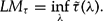
Here, λ = T _Bj/T, j = 1, 2. As shown in Lee and Strazicich (Reference Strazicich and List2003), the critical values for Model C depend on the location of the breaks (λ_j). Therefore, we utilize critical values that correspond to the location of the breaks.

Since only one structural break is found for the sample countries, we will repeat the tests for those countries using the minimum one break LM test as proposed by Lee and Strazicich (Reference Strazicich, Lee and Day2004). We list the null and alternative hypothesis as

(6)

$\begin{equation} \begin{array}{@{}l} {\rm Null}{:}\,y_t = c_0 + d_1 B_{1t} + y_{t - 1} + v_{1t} \\ {\rm Alternative}{:}\,y_t = c_1 + \gamma t + d_1 D_{1t} + \omega _1 DT_{1t} + v_{2t} \\\end{array}\end{equation}$

However, regardless of whether we use the two- or one-break test, if the vector of exogenous variables shows that G t = [1, t]′, then the DGP is the same as that shown in the no-break LM unit root test of the SP test (Lee and Strazicich, Reference Strazicich, Lee and Day2004).Footnote ⁷

3. Data and empirical findings

3.1. Data and variables

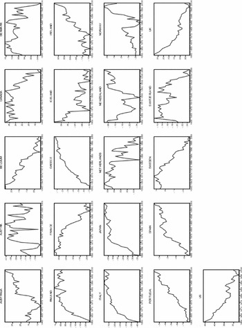
The primary data employed in this paper are annual emissions of CO₂ measured in metric tons per capita.Footnote ⁸ The dataset is based on data for 21 OECD countries that cover the period from 1960 to 2000. Our data were gathered from World Development Indicators published by the World Bank (WDI, 2004). Figure 1 shows the 21 selected OECD countries. While the relative per capita CO₂ emissions for Australia, Canada, and the US are higher, they are lower in Portugal, Spain, and Greece.

Figure 1.

Plots of the relative per capita CO₂ emissions for 21 OECD countries from 1960–2000

How to design a precise examination indicator is the critical key point that has an impact on results. For example, a nice design has been proposed by Carlino and Mills (Reference Carlino and Mills1993), who examined the convergence of US per capita income by calculating the log of the ratio of per capita income relative to the average US per capita income for eight regions of the US and performed a test for a unit root.Footnote ⁹ If we can apply this design from Carlino and Mills (Reference Carlino and Mills1993, Reference Carlino and Mills1996) to our paper, then a unit root implies a non-stationary time series in which shocks to per capita CO₂ emissions relative to the average per capita CO₂ emissions are permanent, meaning that for a shock to CO₂ emissions in each country, there is no tendency for these series to converge toward the average per capita CO₂ emissions (Strazicich and List, Reference Strazicich and List2003). By contrast, a rejection of the unit root implies a stationary series and supports stochastic convergence. We describe a series that is stationary in levels as being I(0).

We follow Strazicich and List (Reference Strazicich and List2003), Nguyen-Van (Reference Nguyen-Van2005), as well as Aldy (Reference Aldy2006), who used Carlino and Mills' (Reference Carlino and Mills1993, Reference Carlino and Mills1996) methodology, in our time series test for convergence in relative per capita CO₂ emissions. In an approach similar to theirs, we calculate a yearly sample average for our 21 OECD countries and then we compute the natural logarithm of relative per capita CO₂ emissions for each country i as follows

(7)

$\begin{equation} y_{\hbox{\scriptsize\it t}}^i = \ln (CO2_{pc_{t}}^i/\hbox{\it averageCO2}_{pc_{t}})\end{equation}$

where $CO{\rm 2}_{pc_{t}}^i$ is the per capita CO₂ emissions for country i and average $CO2}_{pc_{t}}$ is the average value in the sample period. Hence, we use the LM univariate unit root test developed by Lee and Strazicich (Reference Strazicich and List2003) that allows for endogenous structural breaks, which can significantly increase the power of the test for a relative per capita CO₂ emissions series. In addition, the advantage of using the relative per capita CO₂ emissions is that we can utilize them to discuss the convergence effect in an industrialized country. Based on our knowledge, most studies in the literature habitually use the CO₂ emissions in level (total amount or per capita; see McKitrick and Strazicich, Reference McKitrick and Strazicich2005), and this treatment only enables us to look at an individual country, with the observations for relative emissions in all countries in the sample being lacking. Thus, we use the relative emissions per capita, which permit us to avoid some common trends in emissions (Nguyen-Van, Reference Nguyen-Van2005).

Figure 1 plots the values of these series for the 21 countries, indicating that all of these series exhibit trends, but that these trends are mixed.Footnote ¹⁰ The relative per capita CO₂ emissions undulate greatly in Austria, Denmark, the Netherlands, and New Zealand, but most countries exhibit a declining trend in 1990, except for Australia, Greece, Ireland, Italy, Japan, Portugal, and Spain. Furthermore, for Belgium (1951), Canada (1950), France (1957), Iceland (1959), New Zealand (1950), and the US (1950), the series reaches a peak early in the 1950s, but clearly not all countries reach a bottom at the end of the data span, as we can see in the cases of Canada (1998), Iceland (1991), and New Zealand (1979). On the contrary, the countries where a minimum level is reached in the 1950s include Austria (1950), Finland (1950), Italy (1950), Ireland, (1958), Japan (1950), Norway (1950), Portugal (1951), Spain (1951), and Switzerland (1953). Similarly, several countries experience a peak within the sample period, such as Austria in 1991, Finland in 1987, Italy in 1992, Japan in 1995, and Switzerland in 1963. These facts inform us that the relative per capita CO₂ emissions series fluctuate up and down uncertainly, and the turning points are not only one or two but more, since there are also more breaks in the data span.

3.2. Results

For convenience of comparison, in the beginning we perform the traditional unit root tests that do not consider structural change, including the ADF (1979) as well as the Phillips and Perron (Reference Phillips and Perron1988; hereafter PP) unit root tests. However, researchers have conventionally applied the ADF test to examine the stationarity of the variables, regardless of the test's poor power. Elliot et al. (Reference Elliott, Rothenberg and Stock1996; hereafter DF-GLS) and Ng and Perron (Reference Ng and Perron2001) provided different modified unit root tests that are shown to have good power and size, especially in small samples. In their extensive Monte Carlo simulations, Ng and Perron (Reference Ng and Perron2001) found that the $MZ_\alpha ^{GLS}$ and DF-GLS tests achieve better power and size properties than conventional unit root tests (Smyth and Inder, Reference Smyth and Inder2004). Therefore, we apply those statistics to examine the stationarity of the relative per capita CO₂ emissions.

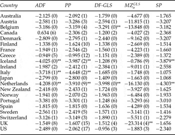
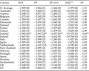
Following the suggestion of Ng and Perron (Reference Ng and Perron2001), the lag order of models is selected based on the modified Akaike information criterion (MAIC). Aside from this, to take advantage of maintaining consistency as much as possible, we also provide the initial LM unit root test without a break as suggested by Schmidt and Phillips (Reference Schmidt and Phillips1992; hereafter SP) in table 1. Consequently, table 1 reports the results of these unit root tests without a break in regressions with constant and trend terms. All of the test results suggest that none of the series is stationary except for Iceland, Italy, and the Netherlands, which reject the null at the 5 per cent level in the ADF and PP tests. The results are similar to Belgium and the Netherlands in the DF-GLS test, but resemble only the UK in the $MZ_\alpha ^{GLS}$ test. Finally, we report that the relative per capita CO₂ series are diverging for all countries, but not in Iceland and the Netherlands, via the SP test. There is an announcement in the unit root tests that relative per capita CO₂ emissions may exhibit the variable I(1). Again, the estimations almost all strongly imply that the time series are non-stationary. However, a key limitation of the five tests is that they do not allow researchers to model the impact of structural changes in the economy.

Table 1.

Unit root tests for relative per capita CO₂ emissions without a break

Notes: DF-GLS and $MZ_\alpha ^{GLS}$ are linear unit root tests provided by Elliot et al. (Reference Elliott, Rothenberg and Stock1996) and Ng and Perron (Reference Ng and Perron2001), respectively. The numbers in parentheses are the lag orders in the ADF and DF-GLS tests. The lag parameters are selected based on the MAIC. Truncation lags are for the Newey–West correction of the PP and $MZ_\alpha ^{GLS}$ tests in parentheses. ** indicates significance at the 5% level.

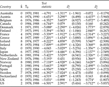
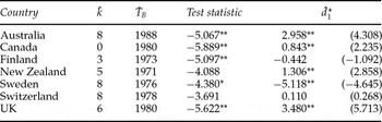
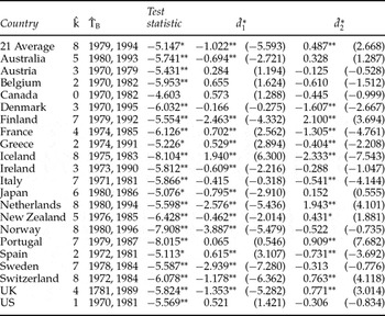
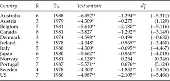
We next utilize Lee and Strazicich's (Reference Lee and Strazicich2003) endogenous two-break minimum LM unit root test to re-examine the relative per capita CO₂ emissions series. Throughout the test, we consider Model C, which allows for two changes in level and trend. Table 2 presents the results, where the estimated breakpoints are shown under the column ‘ $\hat T_B$ ’. We find that almost all relative per capita CO₂ emissions series reject the unit root null at the 10 per cent significance level, except for Australia, Italy, and Switzerland. The evidence provides significant support for relative per capita CO₂ emission stochastic convergence in 18 OECD countries. The examination reveals that two structural breaks in level and/or trend are significant (significant at 10 per cent in an asymptotic normal distribution) in 14 countries, but not in Australia, Canada, Finland, New Zealand, Sweden, Switzerland, and the UK. For these seven countries, a one-break unit root test appears more appropriate. Therefore, we use the one-break minimum LM unit root test developed by Lee and Strazicich (Reference Strazicich, Lee and Day2004). The results are shown in table 3.

Table 2.

Unit root tests for relative per capita CO₂ emissions with two breaks

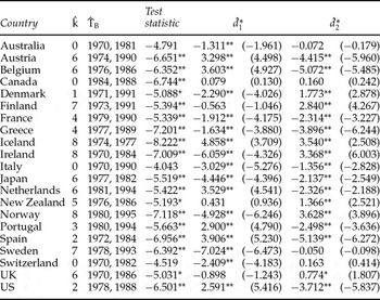
Notes: ** and * denote significance at the 5% and 10% levels, respectively. $\hat k$ is the optimal number of lagged first-differenced terms included in the unit root test to correct for serial correlation. $\hat T_B$ denotes the estimated breakpoints. The 5% and 10% critical values for the minimum LM test with two breaks (Model C) are −5.286 and −4.989, respectively. Standardized coefficients ( $\hat d_j^* = \hat d_j/\hat \sigma)$ ) are reported. T-statistics for $\hat d_j$ = 0 are given in parentheses. The term $\hat d_j$ is the coefficient of the dummy variables under the unit root null in Lee and Strazicich (Reference Strazicich and List2003). The critical values used in this table are from Lee and Strazicich (Reference Strazicich and List2003).

Table 3.

Unit root tests for relative per capita CO₂ emissions with one break

Notes: ** and * denote significance at the 5% and 10% levels, respectively. $\hat k$ is the optimal number of lagged first-differenced terms included in the unit root test to correct for serial correlation. $\hat T_B$ denotes the estimated breakpoints. The 5% and 10% critical values for the minimum LM test with two breaks (Model C) are −4.50 and −4.21, respectively. Standardized coefficients ( $\hat d_j^* = \hat d_j/\hat \sigma)$ ) are reported. T-statistics for $\hat d_j$ = 0 are given in parentheses. The term $\hat d_j$ is the coefficient of the dummy variables under the unit root null in Lee and Strazicich (Reference Strazicich and List2003).

The one-break test results are essentially unchanged from the two break results, except that New Zealand and Switzerland now do not reject the unit root null.Footnote ¹¹ The evidence supports relative per capita CO₂ emission convergence in five industrialized countries, but is lacking in New Zealand and Switzerland. These two countries out of the seven fail to reject the null in the one break test, suggesting that loss of power is not a factor in this case. Regardless of whether there is one break or two breaks existing in the series, we should authentically take into account the breakpoints in our empirical work. As compared to previous univariate time series tests that do not allow for structural breaks, we find stronger support for stochastic convergence.

By comparing the previous literature, Strazicich and List (Reference Strazicich and List2003) examined 21 OECD countries and found evidence supporting convergence in two different model specifications including a cross-section regression test and a panel unit root test. Lanne and Liski (Reference Lanne and Liski2004) estimated structural breaks in a long time series of per capita CO₂ emissions in 16 industrialized nations using the additive outlier model. They found weak general evidence for structural breaks causing downward-sloping per capita emissions during or after the oil-price shocks of the 1970s. Westerlund and Basher (Reference Westerlund and Basher2007) used over a century of CO₂ emissions across 15 countries, and provided overwhelming support in favor of convergence. However, one important point worth noting is that structural breaks were not taken into account in any of those estimations. However, the macroeconomic series are usually affected by exogenous shocks or regime changes in economic events. McKitrick and Strazicich (Reference McKitrick and Strazicich2005) utilized the endogenous two-break minimum LM unit root test to examine the time series properties of historical per capita CO₂ emissions for 121 individual countries from 1950 to 2000, and provided further evidence that the average per capita CO2 emissions of the 121 countries remained stationary with a structural break in 1978. However, for individual countries, their evidence still indicated that the per capita CO₂ emissions for 26 countries were indeed non-stationary. Aldy (Reference Aldy2006) showed that CO₂ emissions appeared to be diverging for OECD countries by means of a large international dataset that comprised an 88-country world dataset using the DF-GLS test. Ezcurra (Reference Ezcurra2007) analyzed the distribution dynamics of per capita CO₂ emissions in 87 countries over the period 1960–1999, using a non-parametric approach that allowed him to study the dynamics of the entire cross-sectional distribution. The results show that cross-country disparities in per capita CO₂ emissions decreased throughout the study period.

An interesting question that arises is related to where we can find the structural breakpoints. We can find the reason for the huge impact of per capita CO₂ emissions in the past, and then refer the corresponding experience that has been accumulated to the administrative authorities, in order to contribute to the establishment of policies in the future. An examination of the breakpoints in table 2 reveals some interesting observations. As expected and similar to Friedl and Getzner (Reference Friedl and Getzner2003) for Austria, the first structural break occurred around the energy crisis period of 1970–1982. This clearly shows that the energy crises had a huge impact on the CO₂ emissions of OECD countries. In addition, the higher oil prices as well as major technological and structural changes such as nuclear power development all reduced the demand for oil and contributed to decreasing emissions from the 1970s onwards (Lindmark, Reference Lindmark2004).

The second structural break occurred during the period 1988–1997. We find that the main reasons for this were that several of the high-income countries were also going through a period of increasing environmental awareness in the 1980s, and the issue induced a turning point (led to a decline) in CO₂ emissions when incomes increased up to a certain level. In other words, this shows that there were growing international concerns that changes in the atmospheric concentrations of a number of gases had the potential to affect the global climate. Therefore, in 1988 the United Nations General Assembly recognized the need to manage human activities that were affecting, or had the potential to affect, the world's climate patterns, prompting the Kyoto Protocol to be negotiated in 1997. Similar to the views put forward by Grubb and Sebenius (Reference Grubb and Sebenius1991) and Welsch (Reference Welsch1993), there have been numerous proposals in the literature on global emission abatement policies since the early 1990s, in which the emphasis has been placed not only on a significant contraction of anthropogenic CO₂ emissions, but also on an equitable per capita distribution of the resulting global carbon budget.

Lanne and Liski (Reference Lanne and Liski2004) reported that industrialized countries have had three phases in their emission development. The first phase was that of rapid growth in per capita emissions, as early industrialization and development in general placed a heavy reliance on solid fuel like coal; however, the CO₂ emissions were mainly from solid fuel consumption. The energy input then gradually changed from coal to oil/gas, and this phase was characterized by less growth in CO₂ emissions. The third phase followed the oil price shocks of the 1970s, which permanently changed the structure of national fuel composition and possibly led to downward sloping per capita emission trends. Similar arguments can be found in McKitrick and Strazicich (Reference McKitrick and Strazicich2005). Therefore, we find some reasonable explanations regarding the large disparities in the breaking points in our sample countries. Nevertheless, in any case, compared with the traditional unit root test that does not allow for structural breaks, we acquire more abundant proof by utilizing the endogenous two-break minimum LM unit root test, in that the relative per capita CO₂ emissions series exhibit stationarity. We also find stronger support for convergence in 21 OECD countries.

3.3. Robustness test

Prior to undertaking the analysis of the relative per capita emissions series, the original per capita emissions series in level along with the average series should be checked for unit roots.Footnote ¹² Tables 4 to 6 therefore present the test results. The 21-country average per capita emission series are displayed in the top row of tables 4 and 5 as ‘21 Average’. Table 4 reports the results of these unit root tests without a break. All of these test results suggest that none of the series is stationary except for Iceland. We then test the two-break LM unit root test in table 5. We find that almost all per capita CO₂ emissions series along with the average series reject the unit root null at least at the 10 per cent significance level, except for Canada. The evidence provides per capita CO₂ emissions in level stochastic convergence in 20 sample countries. Next, for several countries (shown in table 6) the examination reveals that no two structural breaks in level and/or trend are significant, and a one-break unit root test appears to be needed. The results essentially remain the same from the two break results, except that Canada does not reject the unit root null. Overall, the robust test results clearly indicate that most per capita CO₂ emissions along with the average series are stationary and the structural breakpoints nearly match the previous findings.

Table 4.

Unit root tests without a break (original series; robustness test)

Notes: DF-GLS and $MZ_\alpha ^{GLS}$ are linear unit root tests provided by Elliot et al. (Reference Elliott, Rothenberg and Stock1996) and Ng and Perron (Reference Elliott, Rothenberg and Stock2001), respectively. The numbers in parentheses are the lag orders in the ADF and DF-GLS tests. The lag parameters are selected based on the MAIC. The 5% critical value for the SP test is −3.11. The truncation lags are for the Newey–West correction of the PP and $MZ_\alpha ^{GLS}$ tests in parentheses. ** indicates significance at the 5% level.

Table 5.

Unit root tests with two breaks (original series; robustness test)

Table 6.

Unit root tests with one break (original series; robustness test)

Notes: ** and * denote significance at the 5% and 10% levels, respectively. $\hat k$ is the optimal number of lagged first-differenced terms included in the unit root test to correct for serial correlation. $\hat T_B$ denotes the estimated breakpoints. The 5% and 10% critical values for the minimum LM test with two breaks (Model C) are −4.50 and −4.21, respectively. Standardized coefficients ( $\hat d_j^* = \hat d_j/\hat \sigma)$ ) are reported. T-statistics for $\hat d_j$ = 0 are given in parentheses. The term $\hat d_j$ is the coefficient of the dummy variables under the unit root null in Lee and Strazicich (Reference Strazicich and List2003).

4. Policy implications and conclusion

We know that understanding the behavior of the CO₂ emissions series serves as valuable reference to researchers and policy-makers in the formulation of environmental regulations. To perform our tests, we utilize a minimum LM unit root test that endogenously determines structural breaks in both level and trend, as proposed by Lee and Strazicich (Reference Strazicich and List2003, Reference Strazicich, Lee and Day2004), and we link this with the advantage of using relative per capita CO₂ emissions to re-examine the effect of stochastic convergence in an industrialized country. We examine whether the CO₂ emission stochastic effect of convergence hypothesis is supported in countries with the same level of development, i.e. whether or not shocks to relative per capita CO₂ emissions in most industrialized countries are temporary.

Our empirical findings provide significant evidence that relative per capita CO₂ emissions for 21 OECD countries are stochastically converging and exhibit stationarity when we control for breaks, which is in sharp contrast to most findings in the existing literature. When structural breaks are identified in our analysis for each country, the results we obtain contrast with those of other time series tests that do not allow for structural breaks. At the same time, some policy implications are proposed through our observations. Overall, we find that most breakpoints occur around the time of the energy crises as well as in the 1990s.

Since CO₂ emissions are vitally related to energy consumption and industrial production activity, based on the hope that the quality of life will be promoted throughout the world, the issues already referred to above have been leading agenda items in environmental conservation in the past two decades. Most countries have usually adopted counter-plans, such as promoting energy use efficiency, adjusting their energy structure, and changing their industrial structure. By linking these responses and collating our empirical tests through the use of per capita relative CO₂ emissions, most of the series appear to be stationary, exhibiting shocks and only causing short-run deviations around a deterministic trend. In other words, the shocks affect most of the relative per capita CO₂ emissions for the 21 OECD countries only temporarily. This leads us to the following policy implications.

First, shocks to relative series are temporary and soon converge in these industrial countries when we control for breaks based on our results. When the impact is temporary, it might be possible to forecast future movements in the relative per capita CO₂ emissions based on past behavior. Governments should thus pay attention to long-run trends in CO₂ emissions and should not adopt excessive targets or interfere with them in the short run.

Second, when we consider the structural breaks in the historical trends of CO₂ emissions, stationarity can enable each government to estimate the EKC, which will then result in higher accuracy and will not yield spurious regressions. Third, since our unit root tests allow for trending data, our finding of stationary per capita CO₂ emissions is unlikely due to the inclusion or exclusion of a time trend. Fourth, when we find the structural breakpoint, we see the reason why the huge impact of CO₂ emissions was brought about in the past. This then leads to an increase in the experiences accumulated for the administrative authorities, thereby bringing about a great contribution to the establishment of policy in the future.

Fifth, since relative CO₂ emissions exhibit an I(1) series in some sample countries (New Zealand and Switzerland), from another point of view, some of the energy-use policies need to be really improved, including those related to the governmental regulatory inefficiency, heterogeneous preferences among consumers, and relative prices of energy being non-stationary. Finally, when we conduct research in regard to CO₂ emissions in the future – for example, in regard to global warming, and the EKC estimates and expected emissions – we should take into consideration the structural breaks, which can reflect the true current status.

McKibbin and Stegman (Reference McKibbin and Stegman2005) made an interesting claim regarding the notion of the ‘convergence’ of economic variables across countries being a useful concept. They held that if there is empirical evidence of convergence of some economic variables across countries, then our ability to predict the future is enhanced. More generally, Lee et al. (Reference Lee, List and Strazicich2006) also showed that unit roots with breaks, and allowing for breaks in the forecast model, can improve forecast accuracy. Finally, good policy-making typically depends on sound economic forecasts, which can be valuable to policymakers.

As Sathiendrakumar (Reference Sathiendrakumar2003) claimed, the more important matter in relation to this topic is the policy instrument, which should be cost-effective when compared with other policy instruments. This means that maybe we can ask for help from the strength of the market's power to resolve the pollution problem in theory, or make the exterior cost (pollution) convert the inner production burden (the additional production cost) by some limited CO₂ emission policy. The policy instrument should be acceptable to both industry as well as government, and should not directly interfere with production activity and damage economic growth. In addition, the policy instrument should be flexible to changing conditions when handling the pollution question.

Footnotes

¹ We will report the calculation method of the relative per capita CO₂ emissions in equation (7) of section 3.

² Strazicich and List (Reference Strazicich and List2003) examined the CO₂ convergence using the Im et al. (Reference Im, Pesaran and Shin2003, IPS) panel unit root test on the assumption that the individual countries are independent. Nevertheless, Westerlund and Basher (Reference Westerlund and Basher2007) argued that this assumption is based on it being very unlikely to hold in the CO₂ data, combined with a rejection in the test outcome that might be caused by a single converging country. However, as Quah (Reference Quah1997) has repeatedly pointed out in the context of the economic growth literature, this methodology fails to capture a series of potentially interesting features of the evolution of the distribution in question. Aldy (Reference Aldy2006) argued that it even rejects the null hypothesis, as it does not imply that all time series are stationary.

³ List (Reference List1999) indicated that stochastic convergence implies that the effects of temporary shocks dissipate over time, or, likewise, that the time series does not possess a unit root.

⁴ During 1960–2000, there were many environmental protection and climate change agendas that have had a huge impact on energy consumption. For instance, the two oil crises in the 1970s were accompanied by rising energy prices, causing people to switch from the energy that they had been accustomed to using and increasing higher energy use efficiency. The EKC concept then emerged in the early 1990s, whereby the stance adopted was that economic development and environmental quality are conflicting goals. Consequently, most scientists have found it likely that the emissions of CO₂ and other greenhouse gases contribute to global warming (see, for instance, Lanne and Liski, Reference Lanne and Liski2004). Therefore, at the 1992 Earth Summit in Rio de-Janeiro, developed nations agreed to stabilize their greenhouse gas emissions at 1990 levels by the year 2000. In 1997, the Kyoto Protocol was meant to be legally binding and all wealthy nations were called on to reduce greenhouse gas emissions to 6–8 per cent below 1990 levels by 2012. As such, we think that only considering one break seems to be unrealistic.

⁵ Stern et al. (Reference Stern, Common and Barbier1996) indicated that conducting an investigation using the time series data of a single country may be able to account for historic experiences such as an environmental policy and exogenous shocks like energy events.

⁶ For example under a break. Ben-David and Papell (Reference Ben-David and Papell2000) found evidence of multiple breaks in the per capita real GDP of the G7 countries over the past 120 years. Papell et al. (Reference Papell, Murray and Ghiblawi2000) showed more than one structural break in macroeconomic time series data in 16 OECD countries.

⁷ In the SP test with no break, the null hypothesis is y _t=c ₀+y _t−1+v _1t; and the alternative is $y_t = c_1 + \gamma t + v_{2t}$ (Schmidt and Phillips, Reference Schmidt and Phillips1992).

⁸ Per capita numbers give the emissions the same units for large and small countries, and so they control the scale of the economy (Lanne and Liski, Reference Lanne and Liski2004).

⁹ The same enactment method is applied in List (Reference List1999) and Strazicich et al. (Reference Strazicich, Lee and Day2004), who tested for stochastic convergence in 15 OECD countries.

¹⁰ We follow Strazicich and List (Reference Strazicich and List2003) who selected the 21 OECD countries in their studies, but Germany is excluded because there it had significant boundary changes in 1990 (see Strazicich and List, Reference Strazicich and List2003, footnote 4).

¹¹ Strazicich and List (Reference Strazicich and List2003) claimed that many factors may lead to emissions' divergence (like in Australia, Italy, and Switzerland) and also regarded the I(1) series, including governmental regulatory inefficiency, heterogeneous preferences for consumers, and relative prices, as being non-stationary.

¹² The authors are thankful for this suggestion from the anonymous referees.

References

Aldy, J.E. 2006, ‘Per capita carbon dioxide emissions: convergence or divergence?’, Environmental and Resource Economics 33: 533–555.CrossRef Google Scholar

Ben-David, D. and Papell, D.H. 2000, ‘Some evidence on the continuity of the growth process among the G7 countries’, Economic Inquiry 38: 320–330.CrossRef Google Scholar

Böhringer, C. and Welsch, H. 2004, ‘Contraction and convergence of carbon emissions: an intertemporal multi-region CGE analysis’, Journal of Policy Modeling 26: 21–39.CrossRef Google Scholar

Carlino, G.A. and Mills, L.O. 1993, ‘Are US regional incomes converging? A time series analysis’, Journal of Monetary Economics 32: 335–346.CrossRef Google Scholar

Carlino, G.A. and Mills, L.O. 1996, ‘Testing neoclassical convergence in regional incomes and earnings’, Regional Science and Urban Economics 26: 565–590.CrossRef Google Scholar

Dickey, D.A. and Fuller, W.A. 1979, ‘Distribution of the estimators for autoregressive time series with a unit root’, Journal of the American Statistical Association 74: 427–431.Google Scholar

Elliott, G., Rothenberg, T.J., and Stock, J.H. 1996, ‘Efficient tests for an autoregressive unit root’, Econometrica 64: 813–836.CrossRef Google Scholar

Ezcurra, R. 2007, ‘Is there cross-country convergence in carbon dioxide emissions?’, Energy Policy 35: 1363–1372.CrossRef Google Scholar

Friedl, B. and Getzner, M. 2003, ‘Determinants of CO₂ emissions in a small open economy’, Ecological Economics 45: 133–148.CrossRef Google Scholar

Galeotti, M. and Lanza, A. 2005, ‘Desperately seeking environmental Kuznets’, Environmental Modelling and Software 20: 1379–1388CrossRef Google Scholar

Grubb, M. and Sebenius, J.K. 1991, ‘Participation, allocation and adaptability in international tradable emission permit systems for greenhouse gas control’, Paper Prepared for OECD Workshop on Tradeable Greenhouse Gas Permits, Paris, June.Google Scholar

Im, K.S., Pesaran, M.H., and Shin, Y. 2003, ‘Testing for unit roots in heterogeneous panels’, Journal of Econometrics 115: 53–74.CrossRef Google Scholar

Jewell, T., Lee, J., Tieslau, M., and Strazicich, M.C. 2003, ‘Stationarity of health expenditures and GDP: evidence from panel unit root tests with heterogeneous structural breaks’, Journal of Health Economics 22: 313–323.CrossRef Google Scholar PubMed

Kanjilal, K. and Ghosh, S. 2002, ‘Future industrial CO₂ emission and consequences of CO₂ abatement strategies on the Indian economy’, Pacific and Asian Journal of Energy 12: 123–128.Google Scholar

Lanne, M. and Liski, M. 2004, ‘Trends and breaks in per-capita carbon dioxide emissions, 1870–2028’, Energy Journal 25: 41–65.CrossRef Google Scholar

Lee, C.C. and Chang, C.P. 2008a, ‘Unemployment hysteresis in OECD countries: centurial time series evidence with structural breaks’, Economic Modelling 25: 312–325.CrossRef Google Scholar

Lee, C.C. and Chang, C.P. 2008b, ‘Are CO₂ emission levels converging among industrial countries? New evidence from the unit root structural break test’, forthcoming in Applied Economics Letters.CrossRef Google Scholar

Lee, J. and Strazicich, M.C. 2003, ‘Minimum Lagrange Multiplier unit root test with two structural breaks’, Review of Economics and Statistics 85: 1082–1089.CrossRef Google Scholar

Lee, J. and Strazicich, M.C. 2004, ‘Minimum LM unit root test with one structural break’, Appalachian State University, Department of Economics, Working Paper, No. 2004/17.Google Scholar

Lee, J., List, J.A., and Strazicich, M.C. 2006, ‘Non-renewable resource prices: deterministic or stochastic trends?’, Journal of Environmental Economics and Management 51: 354–370.CrossRef Google Scholar

Lindmark, M. 2004, ‘Patterns of historical CO₂ intensity transitions among high and low-income countries’, Explorations in Economic History 41: 426–447.CrossRef Google Scholar

List, J.A. 1999, ‘Have air pollutant emissions converged among US regions? Evidence from unit root tests’, Southern Economic Journal 66: 144–155.Google Scholar

Lumsdaine, R.L. and Papell, D.H. 1997, ‘Multiple trend breaks and the unit-root hypothesis’, The Review of Economics and Statistics 79: 212–218.CrossRef Google Scholar

McKibbin, W.J. and Stegman, A. 2005, ‘Convergence and per capita carbon emissions’, Brookings Discussion Papers in International Economics, No. 167.Google Scholar

McKitrick, R. and Strazicich, M.C. 2005, ‘Stationarity of global per capita carbon dioxide emissions: implications for global warming scenarios’, University of Guelph, Department of Economics, Working paper, No. 2005/03.Google Scholar

Narayan, P.K. 2005, ‘The structure of tourist expenditure in Fiji: evidence from unit root structural break tests’, Applied Economics 37: 1157–1161.CrossRef Google Scholar

Ng, S. and Perron, P. 2001, ‘Lag length selection and the construction of unit root tests with good size and power’, Econometrica 69: 1519–1554.CrossRef Google Scholar

Nguyen-Van, P. 2005, ‘Distribution dynamics of CO₂ emissions’, Environmental and Resource Economics 32: 495–508.CrossRef Google Scholar

Papell, D.H., Murray, C.J., and Ghiblawi, H. 2000, ‘The structure of unemployment’, The Review of Economics and Statistics 82: 309–315.CrossRef Google Scholar

Payne, J., Lee, J., and Hofler, R. 2005, ‘Purchasing Power Parity: evidence from a transition economy’, Journal of Policy Modeling 27: 665–672.CrossRef Google Scholar

Perron, P. 1989, ‘The great crash, the oil price shock and the unit root hypothesis’, Econometrica 57: 1361–1401.CrossRef Google Scholar

Phillips, P.C.B. and Perron, P. 1988, ‘Testing for a unit root in time series regression’, Biometrika 75: 335–346.CrossRef Google Scholar

Quah, D.T. 1997, ‘Empirics for growth and distribution: stratification, polarization, and convergence clubs’, Journal of Economic Growth 2: 27–59.CrossRef Google Scholar

Sathiendrakumar, R. 2003, ‘Greenhouse emission reduction and sustainable development’, International Journal of Social Economics 30: 1233–1248.CrossRef Google Scholar

Schmidt, P. and Phillips, P.C.B. 1992, ‘LM tests for a unit root in the presence of deterministic trends’, Oxford Bulletin of Economics and Statistics 54: 257–287.CrossRef Google Scholar

Sen, A. 2003, ‘On unit-root tests when the alternative is a trend-break stationary process’, Journal of Business and Economics Statistics 21: 174–184.CrossRef Google Scholar

Shafik, N. 1994, ‘Economic development and environmental quality: an econometric analysis’, Oxford Economic Papers 46: 757–773.CrossRef Google Scholar

Smyth, R. and Inder, B. 2004, ‘Is Chinese provincial real GDP per capita nonstationary? Evidence from multiple trend break unit root tests’, China Economic Review 15: 1–24.CrossRef Google Scholar

Stern, D.I., Common, M.S., and Barbier, E.B. 1996, ‘Economic growth and environmental degradation: the environmental Kuznets curve and sustainable development’, World Development 24: 1151–1160.CrossRef Google Scholar

Strazicich, M.C. and List, J.A. 2003, ‘Are CO₂ emission levels converging among industrial countries?’, Environmental and Resource Economics 24: 263–271.CrossRef Google Scholar

Strazicich, M.C., Lee, J., and Day, E. 2004, ‘Are incomes converging among OECD countries? Time series evidence with two structural breaks’, Journal of Macroeconomics 26: 131–145.CrossRef Google Scholar

Sun, L. and Wang, M. 1996, ‘Global warming and global dioxide emission: an empirical study’, Journal of Environmental Management 46: 327–343.CrossRef Google Scholar

Welsch, H. 1993, ‘A CO₂ agreement proposal with flexible quotas’, Energy Policy 21: 748–756.CrossRef Google Scholar

Westerlund, J. and Basher, S.A. 2007, ‘Testing for convergence in carbon dioxide emissions using a century of panel data’, forthcoming in Environmental and Resource Economics.CrossRef Google Scholar

WDI 2004, World Development Indicators, Washington, DC: World Bank.Google Scholar

Zivot, E. and Andrews, D.W.K. 1992, ‘Further evidence on the great crash, the oil-price shock, and the unit-root hypothesis’, Journal of Business and Economic Statistics 20: 25–44.CrossRef Google Scholar