2. Simulation model

The one-dimensional Vlasov–Poisson system is

where the space and time $x$ and $t$ , the electron velocity $v$ , the electron distribution function $f(x,v,t)$ , the electric field $E(x,t)=-\partial _{x}{\it\phi}$ and the corresponding electrostatic potential ${\it\phi}$ have been normalized by the Debye length ${\it\lambda}_{D}=\sqrt{{\it\epsilon}_{0}k_{B}T/n_{0}e^{2}}$ , the inverse plasma frequency ${\it\omega}_{p}^{-1}=\sqrt{m{\it\epsilon}_{0}/n_{0}e^{2}}$ , the electron thermal speed $v_{T}=\sqrt{k_{B}T/m}$ , $k_{B}T/e{\it\lambda}_{D}$ and $k_{B}T/e$ , respectively. Here $-e$ , $m$ , $T$ , $n_{0},{\it\epsilon}_{0}$ and $k_{B}$ are the electron charge, mass, temperature, background density, the vacuum permittivity and Boltzmann constant, respectively. The ions form a uniform neutralizing background.

The evolution of the electron distribution function is followed by numerically solving the Vlasov equation using the standard split method of Cheng & Knorr (Reference Cheng and Knorr1976). Here, advances in the physical and velocity spaces are considered alternately in consecutive time steps. For example, in the first half time step $0<t<{\rm\Delta}t/2$ one advances in the physical space by solving $\partial _{t}\,f+v\partial _{x}\,f=0$ . In the next time step ${\rm\Delta}t/2<t<3{\rm\Delta}t/2$ , one advances the velocity space with $\partial _{t}\,f-E\partial _{v}\,f=0$ . In the following half time step $3{\rm\Delta}t/2<t<2{\rm\Delta}t$ , one again advances the physical space evolution $\partial _{t}\,f+v\partial _{x}\,f=0$ . All equations are solved using the Lax–Wendroff method. For the electric field, the centred-difference form of the Poisson equation is solved in each step using the Thomas algorithm together with Simpson integration. The periodic boundary conditions $f(x,v,t)=f(x+L,v,t)$ and ${\it\phi}(x,t)={\it\phi}(x+L,t)$ , where $L$ is the width of simulated region, are used. For the calculations, the electron distribution satisfies $f(x,v,t)=0$ for $|v|>v_{m}$ , where $v_{m}$ is a cutoff velocity satisfying $1<v_{m}\ll c/v_{T}$ , and $c$ is the speed of light. The number of spatial grid points is $N$ , and the number of velocity grid points is $M$ . The time step $\text{d}t$ satisfies the Courant–Friedrichs–Lewy condition. The numerical code is second-order accurate in time, space, and velocity, and can follow the electron velocity distribution accurately. The parameters $\text{d}t$ , $v_{m}$ , $N$ and $M$ are selected according to the required accuracy, so that they can be different for different parameter regimes. There is no externally supplied initial perturbation of any of the physical variables. That is, the initial perturbations are from the very small but necessarily finite numerical noise. The code has been benchmarked against existing analytical and numerical results on linear and nonlinear Landau damping (Hou, Ma & Yu Reference Hou, Ma and Yu2011b ), as well as high-order plasma wave echoes (Hou, Ma & Yu Reference Hou, Ma and Yu2011a ).

3. Effect of the beam velocity

In a plasma with two counter-streaming electron components, one can expect unstable electrostatic electron oscillations (Hasegawa Reference Hasegawa1968, Reference Hasegawa1971; Clemmow & Dougherty Reference Clemmow and Dougherty1969). To avoid the great variety of possible cases (Clemmow & Dougherty Reference Clemmow and Dougherty1969), we shall restrict ourselves to considering the evolution of two counter-streaming electron plasmas given by the bi-Maxwellian equilibrium distribution function $f_{0}(v)=C(2{\rm\pi})^{-1/2}\exp [-(v-v_{0})^{2}/2]+(1-C)(2{\rm\pi})^{-1/2}\exp [-(v+v_{0})^{2}/2]$ , where $C$ and $1-C$ are the relative concentration of the two plasmas.

Figure 1.

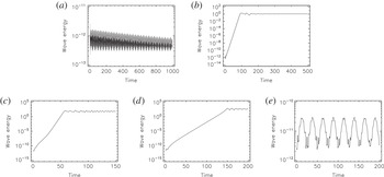
Evolution of the total wave energy for (a) $v_{0}=1$ , $v_{m}=11$ , $\text{d}t=0.001$ , (b) $v_{0}=2$ , $v_{m}=11$ , $\text{d}t=0.001$ , (c) $v_{0}=5$ , $v_{m}=16$ , $\text{d}t=0.0005$ , (d) $v_{0}=10$ , $v_{m}=23$ , $\text{d}t=0.0005$ , and (e) $v_{0}=11$ , $v_{m}=24$ , $\text{d}t=0.0005$ . Here we have assumed $L=20{\rm\pi}$ , $N=1024$ , and $M=3000$ . There is no growth in (a) because the two peaks of the distribution function are too close (i.e. the region with unfavourable gradient is too small Clemmow & Dougherty Reference Clemmow and Dougherty1969).

Figure 1 shows the evolution of the total wave electric field energy ${\it\varepsilon}_{E}=\int _{0}^{L}(E^{2}/2)\,\text{d}x$ for $C=0.5$ (i.e. two identical counter-streaming plasmas) and different values of $v_{0}$ . As mentioned, for efficient and accurate numerical computation, appropriate values for $v_{m}$ and $\text{d}t$ are chosen for each case. Figure 1(a) for $v_{0}=1$ (i.e. in the marginally stable regime) shows that very small-amplitude transient plasma oscillations are initially excited by the noise, which depends on the space–time numerical accuracy, and the wave energy ${\it\varepsilon}_{E}$ gradually damps. Figure 1(b) for $v_{0}=2$ (in the unstable regime) shows that after a short very low level ( ${\sim}10^{-12}$ ) transient stage, ${\it\varepsilon}_{E}$ grows exponentially at a linear growth rate and eventually saturates at a high level ( ${\sim}10^{0}$ ) due to trapping of resonant electrons in the enhanced (nonlinear) wave field. Thereafter it oscillates at the effective bounce frequency of the trapped electrons. Figure 1(c) for $v_{0}=5$ and figure 1(d) for $v_{0}=10$ are similar to figure 1(b), except that here the linear growth stage consists of at least two different rates. As expected, the saturation level depends on the streaming velocity. Finally, figure 1(e) for $v_{0}=11$ shows that ${\it\varepsilon}_{E}$ continues to fluctuate at a very low ( ${\sim}10^{-11}$ ) level.

Figure 2.

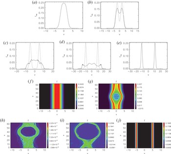
The space-averaged electron distribution function $f_{\mathit{avg}}$ (a–e) and the corresponding phase space $v,x$ (f–j) for, respectively, $v_{0}=1$ , 2, 5, 10, and 11 at $t=1000$ , 500, 140, 200 and $200$ . Here, $f_{\mathit{avg}}=L^{-1}\!\int _{0}^{L}f(x,v)\,\text{d}x$ is the velocity distribution function averaged over $x$ . The dotted line is for the initial distribution $f_{0}(v)=(8{\rm\pi})^{-1/2}\{\exp [-(v-v_{0})^{2}/2]+\exp [-(v+v_{0})^{2}/2]\}$ .

The numerical results can be understood in terms of wave–particle interaction. When $v_{0}$ is very small, the unfavourable gradient $\partial _{v}\,f_{0}(v)$ and the separation of the two peaks in the electron distribution function are small and close to $v=0$ (figure 2 a). Plasma oscillations with such small phase velocities ${\it\omega}_{p}/k$ are of very short wavelengths, so that, in spite of the double-humped distribution function, instability does not occur (Clemmow & Dougherty Reference Clemmow and Dougherty1969) (in the numerical calculation the short-wavelength modes are in fact precluded because of the finite grid size). As a result, the total oscillation energy from the excited plasma oscillations and transients is damped because of numerical dissipation. There is thus little difference between the initial and final distribution functions, as shown in figure 2(a). There are also no trapped particles, as can be seen in figure 2(f). As $v_{0}$ increases, the two peaks of $f_{0}$ move apart, and the region as well as the magnitude of unfavourable gradient increase. Plasma waves with phase velocities in these regions suffer inverse Landau damping and instability appears. Figure 1(b–d) shows that the wave energy initially grows monotonically and eventually saturates, then it oscillates at a certain level. The initial growth in the wave energy is from the electron kinetic energy. Figure 2(b–d) shows that as the energy of the electrons is transferred to the waves, the velocity space distribution of the electrons becomes flattened. As the amplitude of the electric field of the growing waves increases, the electrons in phase with the wave can became trapped. As can be seen in figure 2(g–i), in this saturation stage the acceleration and deceleration of the particles trapped in the wave potential wells lead to the oscillations in the wave energy. However, as can be seen in figure 1(e) for $v_{0}=11$ , the instability disappears when $v_{0}$ becomes too large. Accordingly, there is little difference between the initial and final distribution functions in figure 2(e), and there are no trapped particles in figure 2(j). This is because the instability condition is no longer satisfied, and there are too few electrons in the region of the distribution function with unfavourable gradient, as shall be discussed in more detail below.

Thus, the evolution of the instability without an externally supplied initial perturbation can be separated into three temporal stages, namely the very small transient stage, the instability growth stage, and the saturation stage. In the small transient stage, the initial disturbance is from the numerical noise (and the magnitude is thus dependent on the numerical accuracy). In the next stage the wave electric field grows exponentially since the resonant electrons with velocity larger than the wave phase velocity lose their energy to the waves, resulting in flattening of the affected region of the distribution function. The saturation stage sets in when a sufficient number of resonant electrons become trapped by the enhanced wave electric field and oscillate between the potential walls. Circulation of the trapped electrons in the electron phase space forms vortex-like structures where energy exchange between the wave and the electrons occurs, resulting in the oscillation of wave energy.

Figure 3.

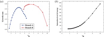
(a) The growth rate versus beam velocity $v_{0}$ and (b) the saturation level of energy versus beam velocity $v_{0}$ as obtained from the simulated wave energy ${\it\varepsilon}_{E}$ . The two branches of the growth rate are due to the non-uniform growth behaviour of the latter, such as in figure 1(c,d).

Figure 1(c,d) for the evolution of the wave energy ${\it\varepsilon}_{E}$ indicates that in the growth stage there can be overlapping of different linear (on the log scale) growth rates. In figure 3(a) we show that the total growth rate as a function of $v_{0}$ can indeed be decomposed into two regimes of $v_{0}$ . In both regimes the growth rates first increase with $v_{0}$ and then decrease, but the corresponding $v_{0}$ regimes are very different. Figure 3(b) shows that the saturation level of the wave energy increases with $v_{0}$ . This is to be expected since in both regimes saturation of the growth is due to electron trapping in the enhanced wave fields. As shall be discussed in more detail in the next section, this behaviour can be attributed to the growth of the different spatial harmonics of the excited waves.

4. Effect of different harmonics

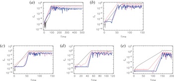
The generation of harmonics during the evolution of beam–plasma or beam–beam instability was pointed out by Yoon (Reference Yoon2000, Reference Yoon2005a ,Reference Yoon b ). In order to see exactly what caused the non-uniform growth of the wave energy for different $v_{0}$ values, we have also carried out fast Fourier transform (FFT) of the wave electric field. Figure 4(a–e) shows how the first four harmonics of the wave electric field (i.e. $E_{k}$ , $k=1,\ldots ,4$ , note the log scale in the figures) are excited and how each grows to saturation, followed by the trapping oscillations. It can be seen that the harmonics and their growth are not necessarily in sequence. When $v_{0}$ is small, in the initial growth stage the higher harmonics can dominate over the fundamental one and their regimes of dominance as well as times of saturation depend strongly but irregularly on $v_{0}$ . The non-uniform growth of the total wave energy in the initial stage found in figure 1(c) can thus be attributed to this growth behaviour of the harmonics. For example, figure 4(a,b) shows that the second harmonic is dominant in the growth stage but the first harmonic becomes dominant in the saturation stage, and their saturation times are quite different. However, when $v_{0}$ is relatively large (figure 4 d,e), the first harmonic is dominant and the higher harmonics are in sequence. The higher harmonics grow at larger rates and saturate at lower levels, which is qualitatively consistent with the result of Yoon (Reference Yoon2005b ). Among a large number of cases simulated, we found in general that the initial growth rate of the wave energy remains constant if and only if a single harmonic turns out to be dominant in the entire growth process, which is consistent with the linear instability theory. Figure 4(c) shows that when two or more harmonics compete, the growth stage of the total wave energy becomes non-uniform in time, as can be expected. The contributions of the different harmonics are also irregular, since they depend on the background and initial conditions as well as the evolution (recall that in the simulation phase space vortices are formed even when the wave amplitude is still very small). For example, we found that in figure 3(a) the second harmonic contributes more to branch A and the first harmonic more to branch B.

Figure 4.

Evolution of the harmonics of the wave electric field for (a) $v_{0}=2$ , $v_{m}=11$ , $\text{d}t=0.001$ , (b) $v_{0}=4$ , $v_{m}=13$ , $\text{d}t=0.0005$ , (c) $v_{0}=5$ , $v_{m}=16$ , $\text{d}t=0.0005$ , (d) $v_{0}=6$ , $v_{m}=18$ , $\text{d}t=0.0005$ , and (e) $v_{0}=10$ , $v_{m}=23$ , $\text{d}t=0.0005$ . The black solid, red dotted, magenta dashed, and blue dash-dot-dot lines are for the first to the fourth harmonics, respectively. The parameters are $L=20{\rm\pi}$ , $N=1024$ , $M=3000$ , and the time step is varied according to the resolution needed.

5. Existence condition of instability

We have shown, by numerically solving the governing equations, that in the evolution of the bi-Maxwellian distribution, beam-type instabilities can take place. Here we consider in more detail the corresponding linear instabilities in terms of eigenmode analysis (Clemmow & Dougherty Reference Clemmow and Dougherty1969).

The general dispersion relation for electrostatic waves in an electron plasma is $D(k,{\it\omega})=0$ , where $k$ is the wave vector, ${\it\omega}={\it\omega}_{r}+\text{i}{\it\gamma}$ is the sum of the wave frequency and growth/damping rate, and (Clemmow & Dougherty Reference Clemmow and Dougherty1969)

For ${\it\gamma}\ll {\it\omega}_{r}$ , ${\it\gamma}$ is given by

so that a mode of frequency ${\it\omega}_{r}$ can grow if $\text{d}_{v}f_{0}(v)>0$ , corresponding to inverse Landau damping. The latter has been attributed to resonant energy exchange with the wave and the electrons with velocities near the wave phase velocity, or $v\sim {\it\omega}_{r}/k$ .

The existence condition and growth rate of the beam instability can be estimated from the cold plasma limit (replacing the Gaussian functions in $f_{0}$ by delta functions) since thermal effects do not contribute significantly to the instability (Clemmow & Dougherty Reference Clemmow and Dougherty1969). The linear dispersion relation for two counter-propagating electron beams is then (Clemmow & Dougherty Reference Clemmow and Dougherty1969; Chen Reference Chen1984; Boyd & Sanderson Reference Boyd and Sanderson2003)

where ${\it\omega}_{pa}=\sqrt{C}{\it\omega}_{p}$ and ${\it\omega}_{pa}=\sqrt{1-C}{\it\omega}_{p}$ are the plasma frequencies of the two beams.

The purely growing beam instability appears for $0<k<k_{cr}$ , where

Physically, this instability is caused by a phase mismatch (due to electron bunching) in the restoring force of the beam-driven electron oscillations, which are thereby destroyed. For the case $C=0.5$ , the beam mode can be written

and the corresponding critical wave vector is $k_{cr}={\it\omega}_{p}/v_{0}$ . In the unstable regime, we can obtain, by setting $\text{d}_{k}{\it\omega}=0$ , the maximum growth rate ${\it\omega}_{p}/2\sqrt{2}$ , occurring for $k=\sqrt{3}{\it\omega}_{p}/2\sqrt{2}v_{0}$ . For the simulation where $L=20{\rm\pi}$ and $M=3000$ , we get $1/10<k<300$ . That is, when $v_{0}=6$ (first harmonic dominates, see figure 4 d)), the growth rate is maximum (figure 3 a), and correspondingly $k\sim 1/10$ .

In the simulations the wavelength of the noise-excited mode is necessarily in the range $2{\rm\pi}/L<k<2M{\rm\pi}/L$ , where $M$ is an integer. The existence condition for instability is then $k_{cr}\geqslant k_{min}$ , where $k_{min}$ is the minimum wave vector allowed in the simulation, that is, $v_{0}\leqslant v_{cr}$ , where the critical velocity is $v_{cr}=(C^{1/3}+(1-C)^{1/3})^{3/2}{\it\omega}_{p}L/4{\rm\pi}$ , or $L\geqslant L_{cr}$ , where the critical system size is $L_{cr}=4{\rm\pi}(C^{1/3}+(1-C)^{1/3})^{-3/2}v_{0}/{\it\omega}_{p}$ .

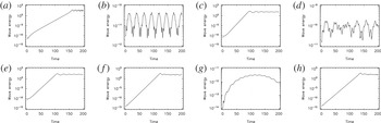
In order to see if these cold-plasma results are applicable to the initial (linear) stage of the instabilities, we have carried out simulations of the instability for several parameter regimes. Figure 1(e) is for $L=20{\rm\pi}$ and $v_{0}=11$ . Since $v_{cr}=10$ , there is no instability, as predicted. Also as expected, figure 5(a,b) shows that with $L=22{\rm\pi}$ instability occurs for $v_{0}=11$ but not for $v_{0}=12$ since here $v_{cr}=11$ . Furthermore, for $C=0.1$ and $L=20{\rm\pi}$ we have $v_{cr}=8.547$ , and figure 5(c,d) shows that instability indeed occurs for $v_{0}=8$ but not for $v_{0}=9$ . Figure 5(e) for $L=22{\rm\pi}$ and $v_{0}=9$ shows that instability occurs since here $v_{cr}=9.4$ . Moreover, for $C=0.2$ and $L=20{\rm\pi}$ , the critical velocity is $v_{cr}=9.3$ and figure 5(f,g) verifies that instability does occur for $v_{0}=9$ but not for $v_{0}=10$ . Finally, figure 5(h) for $L=22{\rm\pi}$ and $v_{0}=10$ shows that instability occurs as expected, since here $v_{cr}=10.24$ . Thus, the simulation results are quite consistent with those from the theory.

Figure 5.

Evolution of the wave energy for (a) $v_{0}=11$ and $L=22{\rm\pi}$ , (b) $v_{0}=12$ and $L=22{\rm\pi}$ , (c) $v_{0}=8$ and $L=20{\rm\pi}$ , (d) $v_{0}=9$ and $L=20{\rm\pi}$ , (e) $v_{0}=9$ and $L=22{\rm\pi}$ , (f) $v_{0}=9$ and $L=20{\rm\pi}$ , (g) $v_{0}=10$ and $L=20{\rm\pi}$ , and (h) $v_{0}=10$ and $L=22{\rm\pi}$ .