1. Introduction
When particles settle through thermal and/or compositional density gradients, double diffusion may fundamentally alter their dynamics. A prime example concerns the outflow of sediments from buoyant, freshwater river plumes into the saline ocean below. In typical estuaries the density contribution of the sediment is less than that of the salinity, so that the overall stratification is stable. Within this overall stable density profile, however, the sediment itself is unstably stratified. Its available potential energy can be released in the form of double-diffusive fingering, which drastically alters the effective settling velocity of the sediment. This effect has been demonstrated in laboratory flow visualization experiments (Green Reference Green1987; Green & Diez Reference Green and Diez1995; Carey Reference Carey1997; Chen Reference Chen1997; Hoyal, Bursik & Atkinson Reference Hoyal, Bursik and Atkinson1999a ,Reference Hoyal, Bursik and Atkinson b ; Maxworthy Reference Maxworthy1999; Parsons & Garcia Reference Parsons and Garcia2000; Parsons, Bush & Syvitski Reference Parsons, Bush and Syvitski2001; Manville & Wilson Reference Manville and Wilson2004). For the purpose of modelling the global sediment cycle, it is essential to have accurate estimates of the sediment flux from river plumes, as rivers represent the main vehicle responsible for the transport of sediment from land into the coastal oceans (Milliman & Syvitski Reference Milliman and Syvitski1992). In spite of its importance, however, a generally accepted comprehensive description of the double-diffusive sediment flux from river plumes is still elusive, and scaling laws and/or reliable quantitative measurements of this sediment flux as a function of the governing flow parameters are as of yet unavailable. Traditionally, this flux has been estimated based on the Stokes settling velocity of the individual sediment grains, without accounting for double-diffusive effects. Our recent linear stability investigation (Burns & Meiburg Reference Burns and Meiburg2012), however, indicates that double-diffusive mechanisms can dominate the dynamics of sediment settling from river plumes. Furthermore, over the last decade theoretical, computational, laboratory and field observations have yielded new and fundamental insight into important aspects of double diffusion. Traxler, Garaud & Stellmach (Reference Traxler, Garaud and Stellmach2012) have developed a unified theoretical framework for the emergence of the collective fingering instability, and the formation of staircases and horizontal intrusions in thermohaline systems. These authors have furthermore confirmed their stability-theoretical scenarios by means of large-scale direct numerical simulations (DNS) (Stellmach et al. Reference Stellmach, Traxler, Garaud, Brummell and Radko2011). Smyth & Kimura (Reference Smyth and Kimura2007, Reference Smyth and Kimura2011) conducted a linear stability analysis and nonlinear, three-dimensional DNS simulations of double-diffusively unstable shear layers, which nicely demonstrate the interaction of Kelvin–Helmholtz and double-diffusive modes during the early stages of the flow. These recent findings raise the question as to how the dynamics of double diffusion may be altered by the presence of a settling velocity.
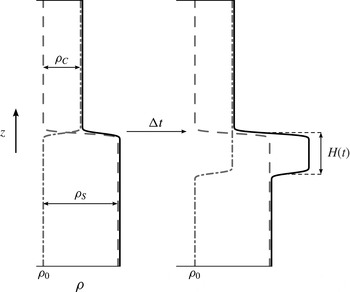
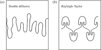
In Burns & Meiburg (Reference Burns and Meiburg2012), we investigated the linear stability of an initial configuration in which a lighter fresh water/sediment mixture is placed above denser saline water. The sediment was modelled as an Eulerian concentration field with a constant settling velocity, and an effective diffusion coefficient smaller than that of the salt. The presence of a settling velocity renders this set-up qualitatively different from the classical double-diffusive configuration of hot, salty water about cold, fresh water, as it results in the formation of a dense ‘nose region’ containing both salt and sediment, cf. figure 1. Thus, this set-up has the potential to generate both double-diffusive and Rayleigh–Taylor-like structures. Figure 2 sketches the unique signatures of the double-diffusive and Rayleigh–Taylor modes for a step change in density at a perturbed interface. The Rayleigh–Taylor mode is dominated by an overturning of the fluid about the density jump while the double-diffusive mode has fingers which are more vertically aligned. However, for stability ratios approaching unity the double-diffusive instability can exhibit more overturning, i.e. appear more Rayleigh–Taylor like. The present investigation examines the formation of both these modes in double-diffusive sedimentation, along with their mutual interactions.
Sketch of density distributions showing the particle (dash-dotted line), salinity (dashed line) and total density (solid line) fields. The density of fresh water is indicated by
 ${\it\rho}_{0}$
. The added density due to salinity,
 ${\it\rho}_{S}$
, is greater than that due to particles,
 ${\it\rho}_{C}$
, which results is an overall stable stratification. After some time
 ${\rm\Delta}t$
, the particles have settled downwards into the upper region of the saline layer, where they form an unstable layer of excess density whose lower boundary is gravitationally unstable.

The flow ‘signatures’ of the two instability modes present in the system. (a) The mostly vertical motion in a double-diffusive instability contrasted against the overturning of the Rayleigh–Taylor instability (b).

By analysing this configuration as a simplified model for the lower boundary of a buoyant river plume, we aim to understand the mechanisms that determine the sediment’s effective settling velocity. The linear stability analysis showed that, depending on the ratio of the nose height to the diffusive interface thickness of the salinity profile, one of two instability modes dominates. For small values of this ratio, the instability mode is primarily double diffusive in nature. For larger values, on the other hand, the particle and salinity interfaces become increasingly decoupled, and the dominant instability mode becomes Rayleigh–Taylor like, centred at the lower boundary of the particle-laden flow region. Scaling laws obtained from the linear analysis were seen to be largely consistent with earlier experimental observations and theoretical arguments put forward by other authors, cf. Green (Reference Green1987), Hoyal et al. (Reference Hoyal, Bursik and Atkinson1999a ,Reference Hoyal, Bursik and Atkinson b ), Maxworthy (Reference Maxworthy1999), Parsons & Garcia (Reference Parsons and Garcia2000) and Parsons et al. (Reference Parsons, Bush and Syvitski2001).
In the present paper, we employ DNS to extend the linear stability investigation of Burns & Meiburg (Reference Burns and Meiburg2012) into the nonlinear regime. In particular, we aim to understand the differences between the ‘fingering’ and ‘leaking’ modes observed in the experiments of Parsons et al. (Reference Parsons, Bush and Syvitski2001), and to establish their relationship to the two linear instability mechanisms mentioned above, namely the double-diffusive and the Rayleigh–Taylor-like modes. Section 2 reviews the governing equations and identifies the governing dimensionless parameters. Subsequently, § 3 describes the numerical approaches employed for solving the two- and three-dimensional problems, respectively, along with the initial and boundary conditions, and it provides validation information. Section 4 initially presents a detailed discussion of two-dimensional simulation results for a low-Schmidt-number case, which is dominated by double diffusion. It then contrasts these with two- and three-dimensional results for a high-Schmidt-number set-up, in order to highlight the differences between double-diffusive and Rayleigh–Taylor-dominated flows, and to establish their relationship with the fingering and leaking modes. Section 5 employs the results of a detailed parametric investigation in order to extract relevant scaling laws, which are subsequently interpreted physically in terms of sediment flux balances. Finally, § 6 summarizes the key results and presents some main conclusions. During the preparation of the present manuscript, we became aware of the related work under submission by Yu, Hsu & Balachandar (Reference Yu, Hsu and Balachandar2014). We would like to acknowledge several helpful discussions with Professor Hsu, especially regarding the effective settling velocity.
2. Problem formulation
2.1. Governing equations
We begin our analysis with the full Navier–Stokes equations in dimensionless form and refer the reader to Burns & Meiburg (Reference Burns and Meiburg2012) for a more complete discussion of the governing equations and the choice of scales:
 $$\begin{eqnarray}\displaystyle & \boldsymbol{{\rm\nabla}}\boldsymbol{\cdot }\boldsymbol{u}=0 & \displaystyle\end{eqnarray}$$
 $$\begin{eqnarray}\displaystyle & \displaystyle \frac{\partial \boldsymbol{u}}{\partial t}+\boldsymbol{u}\boldsymbol{\cdot }\boldsymbol{{\rm\nabla}}\boldsymbol{u}={\rm\nabla}^{2}\boldsymbol{u}-\boldsymbol{{\rm\nabla}}\mathscr{P}+{\it\rho}^{\prime }\frac{\boldsymbol{g}}{g^{\prime }} & \displaystyle\end{eqnarray}$$
 $$\begin{eqnarray}\displaystyle & \displaystyle \frac{\partial S}{\partial t}+\boldsymbol{u}\boldsymbol{\cdot }\boldsymbol{{\rm\nabla}}S=\frac{1}{\mathit{Sc}}{\rm\nabla}^{2}S & \displaystyle\end{eqnarray}$$
 $$\begin{eqnarray}\displaystyle & \displaystyle \frac{\partial C}{\partial t}-V_{p}\frac{\partial C}{\partial z}+\boldsymbol{u}\boldsymbol{\cdot }\boldsymbol{{\rm\nabla}}C=\frac{1}{{\it\tau}\mathit{Sc}}{\rm\nabla}^{2}C. & \displaystyle\end{eqnarray}$$
 $S$
and
 $C$
denote the salinity and sediment concentration, respectively. We have incorporated the base density into the pressure term
 $\mathscr{P}$
and thus only the excess density,
 ${\it\rho}^{\prime }={\it\rho}-1$
, is present in the gravitational term of the Navier–Stokes equation. The characteristic length scale is
 $L^{c}=({\it\nu}^{2}/g^{\prime })^{1/3}$
, the time scale is
 $T^{c}=(L^{c2}/{\it\nu})$
and the reduced gravity is
 $g^{\prime }=({\it\gamma}{\rm\Delta}C)g$
. The salinity and sediment concentration fields are scaled by their respective maximum differences, i.e.
 ${\rm\Delta}S$
and
 ${\rm\Delta}C$
. As seen in (2.1)–(2.4), application of the characteristic scales results in the creation of four dimensionless groups:
 $$\begin{eqnarray}\displaystyle & \displaystyle V_{p}=\frac{V_{st}}{({\it\nu}g^{\prime })^{1/3}}, & \displaystyle\end{eqnarray}$$
 $$\begin{eqnarray}\displaystyle & \displaystyle R_{s}=\frac{{\it\alpha}{\rm\Delta}S}{{\it\gamma}{\rm\Delta}C}, & \displaystyle\end{eqnarray}$$
 $$\begin{eqnarray}\displaystyle & \displaystyle \mathit{Sc}=\frac{{\it\nu}}{{\it\kappa}_{s}}, & \displaystyle\end{eqnarray}$$
 $$\begin{eqnarray}\displaystyle & \displaystyle {\it\tau}=\frac{{\it\kappa}_{s}}{{\it\kappa}_{c}}. & \displaystyle\end{eqnarray}$$
 $R_{s}$
and
 $\mathit{Sc}$
are the stability ratio and the Schmidt number, respectively, as defined in the salt finger literature (Huppert & Manins Reference Huppert and Manins1973). The dimensionless settling velocity,
 $V_{p}$
, is based on the Stokes settling velocity,
 $V_{st}$
, of an individual particle. Lastly, the diffusivity ratio
 ${\it\tau}$
is the inverse of the typical diffusivity ratio used in the salt finger literature. In this work, we make the assumption that sediment diffuses much more slowly than salinity. This assumption is based on the Einstein–Stokes diffusion coefficient for a settling particle and is investigated more thoroughly in Burns & Meiburg (Reference Burns and Meiburg2012). For the nonlinear simulations to be discussed below, we aim to employ a sufficiently large value of
 ${\it\tau}$
so that any further increase in
 ${\it\tau}$
would not significantly change the results. At the same time, numerical considerations prevent us from using excessively large values of
 ${\it\tau}$
. Our earlier linear stability analysis suggests that
 ${\it\tau}=25$
satisfies both of these conditions, so that we will employ it throughout the investigation. Hence, the simulations to be discussed in the following should be viewed as an effort to investigate the influence of
 $V_{p}$
,
 $R_{s}$
and
 $\mathit{Sc}$
on double-diffusive sedimentation, in the limit of slowly diffusing sediment. We do want to mention, however, that empirical relations between sediment grain size, settling velocity and diffusivity are available (e.g. Segre et al.
Reference Segre, Liu, Umbanhowar and Weitz2001) and could be employed in follow-up studies.
2.2. Two-dimensional flow formulation
To simulate two-dimensional flows, a streamfunction-vorticity formulation is used in place of primitive variable formulation. The result is that (2.1) and (2.2) will be replaced by their streamfunction-vorticity counterparts:
 $$\begin{eqnarray}\displaystyle & \displaystyle \boldsymbol{u}=\left(\frac{\partial {\it\psi}}{\partial y},-\frac{\partial {\it\psi}}{\partial x}\right), & \displaystyle\end{eqnarray}$$
 $$\begin{eqnarray}\displaystyle & {\it\omega}=\boldsymbol{{\rm\nabla}}\times \boldsymbol{u}, & \displaystyle\end{eqnarray}$$
 $$\begin{eqnarray}\displaystyle & {\it\omega}=-{\rm\nabla}^{2}{\it\psi}, & \displaystyle\end{eqnarray}$$
 $$\begin{eqnarray}\displaystyle & \displaystyle \frac{\partial {\it\omega}}{\partial t}+\boldsymbol{u}\boldsymbol{\cdot }\boldsymbol{{\rm\nabla}}{\it\omega}={\rm\nabla}^{2}{\it\omega}-\frac{\partial {\it\rho}^{\prime }}{\partial x}\frac{g}{g^{\prime }}. & \displaystyle\end{eqnarray}$$
2.3. A note on the Rayleigh number
Some readers may note the lack of a Rayleigh number, which is ubiquitous in buoyancy-driven flows. This is a result of choosing an intrinsic length scale based on viscosity, instead of imposing a length scale associated with our computational domain. Put another way, the characteristic length scale is chosen as the distance which creates a sediment Grashof number of unity:
 $$\begin{eqnarray}\mathit{Gr}_{c}=\frac{g{\it\gamma}{\rm\Delta}CL^{c3}}{{\it\nu}^{2}}=1.\end{eqnarray}$$
One can relate the Grashof to the Rayleigh number through the Schmidt number and the stability ratio (given a Rayleigh number based on salinity):
 $$\begin{eqnarray}\mathit{Ra}_{s}=\frac{g{\it\alpha}{\rm\Delta}SL^{c3}}{{\it\nu}{\it\kappa}_{s}}=\mathit{Sc}R_{s}.\end{eqnarray}$$
Consequently, while our governing equations lack a Rayleigh number, one can be defined based on any relevant length scale in the problem. One could define a Rayleigh number for the sediment field based on the half-height of the computational domain as
 $\mathit{Ra}_{c}=\mathit{Sc}H^{3}$
, where
 $H$
is made dimensionless by
 $L^{c}$
. A similar number can be constructed for the salinity field,
 $\mathit{Ra}_{s}=R_{s}\mathit{Sc}H^{3}$
. These Rayleigh numbers are based on the entire box height and as such provide a reference for the range of scales that will develop within the domain. Perhaps a Rayleigh number more relevant to the driving force of motion is one based on the interface thickness, thus incorporating a measure of the density gradient which drives flow into the Rayleigh number. However, the interface thickness is a time-dependent quantity and thus the result of a simulation, while a Rayleigh number based on the domain half-height is an input into the simulation.
3. Numerical methods
To study these flows we use DNS in two and three dimensions. The two primary requirements in choosing a numerical method for the present study are, first, the ability to resolve sharp gradients and, second, the ability to accurately capture the spectral properties of the flow. The need to resolve sharp gradients is primarily due to the high
 $\mathit{Sc}$
and
 ${\it\tau}$
values to be studied. Spectral properties are important for a variety of reasons, among them comparing growth rates against linear stability predictions, understanding the evolution of length scales (wavenumbers) in the nonlinear phase of the flow as well as gaining insight into the difference between fingering and leaking modes, as seen in the experiments of Parsons et al. (Reference Parsons, Bush and Syvitski2001). Along these lines, two numerical schemes have been chosen; one each for two- and three-dimensional flows.
3.1. Two-dimensional flow solver
As stated earlier, the streamfunction-vorticity formulation is used for two-dimensional flows. To solve these equations, a hybrid pseudospectral, compact finite-difference spatial scheme is combined with the low-storage Runge–Kutta/Crank–Nicolson time stepping of Williamson (Reference Williamson1980). The pseudospectral method is used in the horizontal (periodic) direction. To deal with sharp gradients, the code is capable of using either a uniform or a stretched grid in the vertical direction. We discretize the vertical direction using a compact finite difference method (Lele Reference Lele1992) of up to eighth order in the interior and fourth order at the boundaries. We do not expect the lower order at the boundaries to degrade the overall solution accuracy since we stop any simulations before the evolving flow structures reach the upper/lower walls. For a more detailed description of the code and its methods, we refer the reader to Burns (Reference Burns2013).
3.2. Three-dimensional flow solver
For the simulation of three-dimensional flows, we use the flow solver IMPACT, developed by Rolf Henniger at ETH-Zurich. The solver is so named because it solves Incompressible flows on Massively PArallel CompuTers. The implementation and validation details of this flow solver have been published elsewhere (Henniger Reference Henniger2011; Henniger, Obrist & Kleiser Reference Henniger, Obrist and Kleiser2012) and the reader is encouraged to seek out these references as desired. For the purposes of this work, a brief description of the code will suffice.
IMPACT uses a primitive variable formulation on a structured mesh. Within a single cell, the variables are staggered, with velocity nodes centred on the face normal to their direction of propagation and pressure/scalars located at the cell centre. The solver uses central finite differences in all spatial directions with the accuracy capability ranging from second order up to tenth order compact. For this work, a non-compact sixth-order scheme is chosen for all three-dimensional simulations. The improved accuracy and spectral resolution characteristics of staggered grids (Lele Reference Lele1992) dictate that compact schemes are unnecessary. For temporal differencing, the low-storage third-order Runge–Kutta/Crank–Nicolson scheme of Wray (Reference Wray1986) is used. The pressure is solved using the Schur complement formulation, and at each Runge–Kutta substep a Richardson iteration is used to ensure convergence of the pressure field. Linear systems are solved by the BiCGStab algorithm with a multigrid preconditioner.
3.3. Initial and boundary conditions
The flow field is initially quiescent and as such, the flow is driven by the potential energy stored in the initial density profile. The initial profile for the sediment concentration field is a step profile which has been made smooth using an error function
 $$\begin{eqnarray}C(x,y,z,0)=0.5\left(1+\text{erf}\left(\frac{z-{\it\delta}(x,y)}{l_{0}}\right)\right).\end{eqnarray}$$
Here,
 ${\it\delta}(x,y)$
is an initial perturbation whose spectral characteristics are specified and
 $l_{0}$
is the initial thickness of the profile. The salinity profile is defined to be the opposite of the sediment in that
 $S(x,y,z,0)=1.0-C(x,y,z,0)$
.
The boundary conditions in the horizontal directions (
 $x,y$
) are periodic. In the vertical direction (
 $z$
), the walls are slip walls with no penetration, i.e.
 $\partial u/\partial z=\partial v/\partial z=0$
and
 $w=0$
. The salinity field utilizes a no-flux condition at both the top and bottom walls,
 $\partial S/\partial z=0$
. For the sediment field, the top wall uses a no-flux boundary condition formulated with respect to the settling velocity while the bottom wall sets the diffusive flux equal to zero
 $$\begin{eqnarray}\displaystyle & \displaystyle V_{p}C-\frac{1}{{\it\tau}\mathit{Sc}}\frac{\partial C}{\partial z}=0\quad \text{at top wall} & \displaystyle\end{eqnarray}$$
 $$\begin{eqnarray}\displaystyle & \displaystyle \frac{\partial C}{\partial z}=0\quad \text{at bottom wall}. & \displaystyle\end{eqnarray}$$
3.4. Validation
In this section, we compare the linear growth regime of small perturbations in both the two- and three-dimensional solvers to the linear stability predictions from Burns & Meiburg (Reference Burns and Meiburg2012). This comparison is two-fold; first, it is a side-by-side comparison of the two flow solvers and second, it is a comparison of fully nonlinear flow development with the linear stability predictions. Before proceeding, we must revisit the quasi-steady-state approximation (QSSA) that was invoked by Burns & Meiburg (Reference Burns and Meiburg2012) when performing a stability analysis on a non-stationary base state. In their linear stability calculations, static values of the interface thickness,
 $l_{s}$
and
 $l_{c}$
, are used, when in reality these values are evolving in time. Thus, comparisons between linear and nonlinear growth rates should be viewed with this limitation in mind.
We choose two flows which have an order of magnitude difference in the Schmidt number, in order to see the influence of interface diffusion on the growth of the perturbations. The two simulations share many parameters:
 $x,y\in [0,L)$
,
 $z\in [-L,L]$
,
 $N_{x}=N_{y}=128$
,
 $N_{z}=385$
,
 $V_{p}=0$
,
 $R_{s}=2$
and
 $l_{s0}=l_{c0}=1.5$
. The two parameter sets will be referred to as ‘large
 $\mathit{Sc}$
’ and ‘small
 $\mathit{Sc}$
’ and have distinct parameters values of
 $\mathit{Sc}=10$
,
 ${\it\tau}=10$
,
 $L=28.13$
and
 $\mathit{Sc}=1$
,
 ${\it\tau}=100$
,
 $L=20$
, respectively. The simulations are seeded with a spectral perturbation which has a Gaussian distribution centred at
 $k_{max}=3$
with a narrow bandwidth
 ${\it\sigma}_{pert}=0.35$
to minimize any competing modes. In addition, the three-dimensional perturbation has a randomized phase angle to ensure full three-dimensionality. The perturbation field is then scaled to have a mean-squared displacement value of
 $5\times 10^{-7}$
, chosen to be small in order to minimize nonlinear effects.
Three different flow metrics were measured at the initial interface location (
 $z=0$
): the magnitude of the sediment fluctuations,
 $\langle C^{\prime 2}\rangle$
; the energy contained in the perturbed mode,
 $\Vert {\hat{C}}_{k,max}\Vert$
; and the magnitude of the kinetic energy fluctuations,
 $\langle u_{i}^{\prime }u_{i}^{\prime }\rangle$
. As a note, the bracket notation
 $\langle \cdot \rangle$
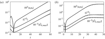
refers to averaging of all horizontal directions and the prime notation is the local deviation from the horizontal average. The growth of these quantities with time is shown in figure 3 for both the large- and small-Schmidt-number cases. The values themselves have been scaled in order to fit in the same window.
Linear growth region for both
 $\mathit{Sc}=10$
(a) and
 $\mathit{Sc}=1$
(b). Good agreement is seen between the two- (solid curves) and three-dimensional (dotted curves) simulations. The growth rates are in line with linear stability predictions, see the text for a more thorough discussion.

The most obvious feature is the agreement between the two- and three-dimensional data throughout the linear range. Even the kinetic energy, which shows a strong dip before the linear growth regime, is captured almost identically by the two solvers. The first sign of diverging results is seen at the end of the linear regime and is clearest for the smaller Schmidt number (right frame). Although expected, we also see that the sediment fluctuation curve follows almost the exact same path as the spectral energy of the perturbed mode, telling us that the perturbed mode remains the dominant mode throughout the linear growth. For
 $\mathit{Sc}=10$
, the slope of the linear region is 0.122, based on the spectral energy. However, the spectral energy is related to the square of the spectral coefficient,
 $\Vert {\hat{C}}_{k}\Vert \sim \text{e}^{2{\it\sigma}t}$
, and thus the growth rate based on the nonlinear simulations is
 ${\it\sigma}_{nl}=0.061$
. Although initially
 $l_{s}=1.5$
, it is clear that there is a period of time during which the eigenmodes are setting up before linear growth occurs. The earliest point of linear growth is
 $t\approx 10$
, which has
 $l_{s}=2.5$
and a linear stability growth rate of
 ${\it\sigma}_{ls}=0.055$
. However, the salinity interface thickness continues to grow throughout this simulation, and thus so does the linear stability growth rate prediction. As an example, at
 $t=40$
and
 $l_{s}=4.27$
the predicted growth rate would be
 ${\it\sigma}_{ls}=0.067$
. Clearly, the nonlinear growth rate, which should be viewed as the more correct prediction, is within the range of values predicted from linear stability theory. Similarly, for
 $\mathit{Sc}=1$
, the growth rate from the nonlinear simulations is
 ${\it\sigma}_{nl}=0.164$
while the range of linear stability predictions is
 $0.155\leqslant {\it\sigma}_{ls}\leqslant 0.175$
. The good agreement between the growth rates predicted by linear theory and those observed in the DNS simulations furthermore provides a posteriori justification of the QSSA made in the former.
4. Direct numerical simulations
4.1. Two-dimensional flow development
We begin with an examination of the qualitative aspects of the flow. Our primary concern is to understand how particle settling affects the flow, with a secondary emphasis on the role of the Schmidt number and stability ratio, since they strongly influence the intensity of the double-diffusive instability. Throughout this section, we examine one representative flow, in two dimensions, with parameter values of
 $V_{p}=0.04$
,
 $\mathit{Sc}=0.7$
,
 $R_{s}=2$
and
 ${\it\tau}=25$
. To provide some physical context to these values, assuming typical ocean salinity loading of 2–3 % the value
 $R_{s}=2$
corresponds to roughly
 $20\ \text{kg}\ \text{m}^{-3}$
of sediment and
 $V_{p}=0.04$
corresponds to slightly smaller than a particle radius of
 $10\ {\rm\mu}\text{m}$
. For the range of settling velocities investigated in this work, the sediment particles all fall within the classification of clays to the finer silts. Further below, we will discuss results from a parametric study, in which we explored the influence of the governing dimensionless parameters, in particular the Schmidt number, the settling velocity and the stability ratio. Specifically, we investigate stability ratios ranging from 1.1 to 8, corresponding to sediment concentrations ranging from 5 to
 $36\ \text{kg}\ \text{m}^{-3}$
. Mulder & Syvitski (Reference Mulder and Syvitski1995) list average yearly sediment concentration values in the range of
 $10{-}40\ \text{kg}\ \text{m}^{-3}$
for a number of ‘dirty’ rivers in various regions around the world, and values in the range of
 $0.1{-}7\ \text{kg}\ \text{m}^{-3}$
for many additional ‘moderately dirty’ rivers. This indicates that our simulations primarily apply to such rivers.
We remark that the Schmidt number for salt and water is approximately 700, which is much larger than the values employed here. While numerical considerations prevent us from conducting simulations for
 $\mathit{Sc}=700$
, the physical mechanisms to be explored below are potentially also relevant to a warm river outflow into a cold lake (
 $\mathit{Sc}=7$
), or to the settling of small water droplets through a temperature gradient in air (
 $\mathit{Sc}=0.7$
). Since we apply
 ${\it\tau}=25$
throughout this investigation, our simulations most closely apply to fine sediment particles, which have an effective diffusivity much smaller than that of salt. As a final comment, the initial perturbation in the DNS simulation is much larger than that used in § 3.4, thus the time scales seen in figure 3 will not reflect those seen in later figures.
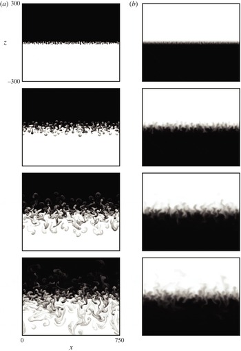
Figure 4 shows the sediment and salinity fields for four different time levels. The entire horizontal extent of the domain is shown in each frame, however the domain has been truncated in the vertical direction to show only the most active portion. The top two frames show the early development of the instability. The interface is initially displaced by a random perturbation but develops a definite preferred wavelength. The instability is beyond the linear stage, yet the fingers are still quite uniform with regular spacing. While the first sediment/salinity pair shows a clear dominant wavelength, the second and third pairs show an increasing influence from additional wavelengths. These two time levels also show the emergence of a secondary instability acting on the fingers (Stern Reference Stern1969).
Snapshots of the sediment (a) and salinity (b) concentration profiles at times
 $t=40$
, 100, 200 and 300 (top to bottom). Parameters:
 $V_{p}=0.04$
,
 $\mathit{Sc}=0.7$
,
 $R_{s}=2$
and
 ${\it\tau}=25$
.

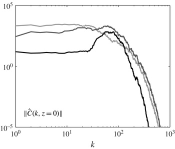
In his work, Stern examined a field of uniform salt fingers within a linearly stratified environment, which, absent any boundaries, will satisfy the equations of motion. This flow has a one-dimensional (vertical) velocity field with variations to the velocity, salt and temperature profiles in the horizontal directions only. He found that the flow would be unstable to large-scale velocity perturbations, e.g. gravity waves, and uses the term ‘collective’ instability to describe the transfer of energy from the motion of the salt fingers as a group to the larger-scale perturbation in the flow. However, in more recent years the term collective instability has come to be associated specifically with gravity waves within the double-diffusive literature and as such we will use the more general term secondary instability in this work. Such a secondary instability is evident when looking at the spectral composition of our sample flow, plotted in figure 5, which shows a gradual shift of energy to longer wavelengths. However, the figure does not allow us to draw any conclusions about the precise form of this collective instability, i.e. whether or not it corresponds to a gravity wave. The version of the instability seen in our figure 4 also differs from that described by Stern in that the fingers only occupy a finite vertical region of the domain, due to the initial step-like base concentration profiles. The collective motion of the fingers remains unstable but, to borrow wording from Stern, results in only one ‘discontinuous’ fingering layer with the ‘convective mixing’ layers occupying all space above and below.
The energy spectra of the sediment field taken at
 $z=0$
and at times
 $t=20$
(black trace),
 $t=40$
(dark grey trace) and
 $t=100$
(light grey trace). The gradual shift of energy to longer wavelengths is indicative of a secondary instability.

The final snapshot shows the vigorous motion at the interface as well as the release of positively and negatively buoyant plumes. From here onwards, we use the term ‘plume’ to denote a blob of fast moving fluid which is no longer anchored to the interfacial finger. At time
 $t=200$
, the first plumes can be seen to detach themselves from the active fingers and begin to accelerate away from the interface. Once salinity diffusion has equilibrated the finger with the surrounding fluid, the density difference between the two is largely due to variations in the slowly diffusing particle concentration field, so that it remains relatively constant. This results in an acceleration phase during which the plume increases in velocity until viscous effects or entrainment compensate the buoyancy difference. In addition, the process of distinguishing individual plumes becomes more difficult at later times, e.g.
 $t=300$
, as trailing plumes are able to catch up with leading plumes by moving into their wake region. This results in a multicap structure wherein the leading plume widens in the horizontal and thins in the vertical direction after the impact by the trailing plume, which itself spreads but to a lesser degree. The collision of plumes is one of the major ways in which kinetic energy is generated in the system, as will be seen later in the text.
4.1.1. The interface region
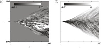
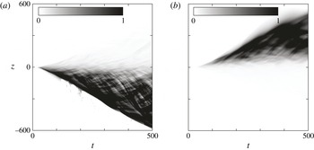
Additional insight into this flow can be gained by averaging in the horizontal directions and then visualizing the averaged profile over time. A natural choice for this type of analysis would be either one of the scalar fields; however, the visualization of such fields is difficult because the interesting flow features move into a background stratification set by the initial conditions. A better choice is to remove the problem of background stratification by visualizing the fluctuations, e.g.
 $\langle C^{\prime 2}\rangle$
. Figure 6 shows the horizontal averaged r.m.s. fluctuations for both the sediment (a) and salinity (b) fields.
Time variation of two-dimensional, horizontally averaged sediment (a) and salinity (b) r.m.s. fluctuations. Same parameters as figure 4.

These plots illustrate important phenomena which occur in the flow; the most striking being the thickening of the fingering interface, marked by the region of strongest fluctuations. Starting from
 $t=0$
, the sediment fluctuations grow sharply from a very narrow region to a significant thickness. This central region remains the location of the largest fluctuations throughout the entire simulation. The salinity fluctuations show similar behaviour but with a magnitude less than half that of the sediment. As will be seen later, this fingering region also manifests itself as an increase in the interfacial thickness of the horizontally averaged, total (non-fluctuating) sediment and salinity fields. Contrast that to the sharp gradient retained in the fingers of figure 4, even at late times.
An indicator of the secondary instability is the transition at
 $t\approx 50$
from a smooth to a rough fingering region, which represents the shift from (almost) uniform to very non-uniform individual fingers. The plot also shows the presence of plumes in the form of the dark, streaked areas. Most of the streaks share a similar slope which is suggestive of a characteristic rise (fall) velocity among positively (negatively) buoyant plumes. The salinity profile shares many features with the sediment profile; however, the magnitude of those features are much smaller, most likely due to the faster diffusion of salinity.
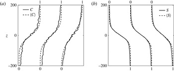
In addition to qualitative analysis, the features seen in figure 6 can be measured quantitatively. We can extract both the thickness of the interfacial region as well as its position by taking a least-squares fit of the average profile to an error function.
 $$\begin{eqnarray}\langle C\rangle _{fit}(z,t)=0.5\left(1+\text{erf}\left(\frac{z-z_{c}(t)}{l_{c}(t)}\right)\right).\end{eqnarray}$$
Here,
 $z_{c}$
represents the location at which
 $\langle C\rangle _{fit}=0.5$
and henceforth we will refer to this location as the interface of the averaged profile. The thickness of the average profile is represented by
 $l_{c}$
. Similar values are defined for the salinity field but with a minus sign before the error function, reflecting the different orientations of the fields. Figure 7 confirms the validity of such an error function fit.
Comparison of the error function fit (dashed line) to the mean scalar field (solid line) for sediment (a) and salinity (b). A good fit is most crucial in the region approximately
 $z=0$
, and consequently this region is weighted more heavily than the end points of the profile. The fit is shown for times
 $t=(300,400,500)$
, with the curves being offset so as to not overlap.

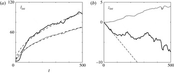
The time evolution of the thickness and location values for both interfaces is shown in figure 8. One of the most striking features is that the sediment interface is more diffuse than the salinity interface. It should be noted that the interface thickness is derived from the average scalar profile, however this observation is counter to the fact that the molecular diffusion of salinity is 25 times larger than its sediment counterpart. Fitting the interfacial thickness to a diffusive
 $t^{1/2}$
profile results in an effective diffusivity ratio of approximately 0.5, i.e. as a result of double-diffusive sedimentation the sediment effectively diffuses twice as fast as the salinity.
(a) The interface thickness for both sediment (black trace) and salinity (grey trace). The dashed lines represent the least-squares fit of the interface thickness to a
 $t^{1/2}$
diffusive behaviour, see the text for details. (b) The interface position with same legend, except here the dashed line represents the constant Stokes settling velocity.

A feature that stands out in both plots is the fluctuating nature of the sediment interface, visible in both the thickness and location. It is likely that these fluctuations are caused by the vigorous motion of the fingers, and that they are enhanced by the two-dimensionality of the simulations. The latter assumption will be tested in § 4.2 where we present comparisons with three-dimensional simulations. Another interesting, and rather surprising, feature is the upward motion of the salinity interface. We expect the sediment interface to move downward as a result of particle settling, and initially it does move at precisely the Stokes settling speed. However, after the instability has grown to a significant size, near
 $t\approx 100$
, the sediment interface location begins to deviate significantly from that predicted by the Stokes settling velocity. In summary, both interface positions exhibit unexpected behaviour.
To better understand the evolution of the interfaces, it is useful to analyse the height difference between the interfaces. Physically, this height difference represents the ‘nose region’,
 $H=z_{s}-z_{c}$
, where both salinity and sediment are present in high concentrations and where a locally unstable stratification can occur. Relating back to the Rayleigh–Taylor instability, the stable salinity interface acts as a ‘lid’ on the vorticity generated at the unstable interface, so that the instability along the lower, unstable interface can become stronger as the nose region becomes larger. The other half of the explanation relates to the thickness of the salinity interface,
 $l_{s}$
, which is the major factor determining the strength of the double-diffusive instability (especially in systems with large
 ${\it\tau}$
). Figure 8 shows that both
 $H$
and
 $l_{s}$
grow with time, with
 $l_{s}$
always substantially larger than
 $H$
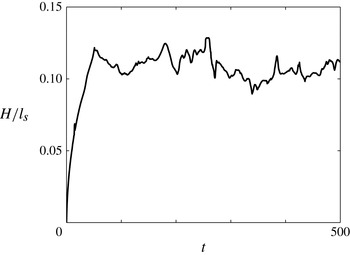
, so that the nose region remains embedded within the larger region of the salinity gradient. Results from Burns & Meiburg (Reference Burns and Meiburg2012) suggest that under such conditions, double-diffusive effects are important. Once the instability is fully developed, the ratio
 $H/l_{s}$
remains remarkably constant, cf.figure 9.
The ratio of the nose region height,
 $H=z_{s}-z_{c}$
, to the salinity interface thickness,
 $l_{s}$
.

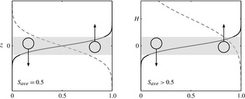
The physical mechanism responsible for the upward migration of the salinity interface can be traced back to the loss of symmetry between upward and downward moving fingers caused by the offset between the interfaces. Figure 10 shows a schematic of the fingering region, shaded grey, for two cases; one where the interfaces are colocated and a second with the salinity interface displaced. Key to this concept is the average salinity value,
 $S_{ave}$
, in the shaded region where the fingers originate, as well as the salinity values above and below the shaded region, where
 $S=0$
and
 $S=1$
, respectively. For a symmetric case,
 $S_{ave}=0.5$
in the shaded region, so that both upward and downward moving fingers have the same
 ${\rm\Delta}S$
between where they originate (grey region) and where they end up. When the symmetry is broken, this picture changes. The fingering process now effectively mixes a region in which the average salinity is larger than 0.5, so that the
 $S=0.5$
contour is displaced upwards. As a side effect of this symmetry breaking in the salinity flux, the salinity profile will develop asymmetrically, i.e. it will be steeper for smaller salinity concentration values and smoother for larger salinity values.
Cartoon schematic illustrating the upward motion of the salinity interface caused by the loss of symmetry of upward and downward moving fingers. This schematic is drawn in a reference frame moving with the sediment interface. See the text for a complete description.

In the above process, the settling velocity of the sediment plays two important roles. First, the initial settling, which occurs before the instability has developed, creates the offset between the sediment and salinity profiles which subsequently drives this process. We note that the upward motion of the salinity interface is not contingent on a settling velocity, only on the offset. Separate simulations with no settling, but with an initial offset, have confirmed that the upward motion of the salinity interface still persists. However, in such cases, the sediment interface will eventually track upwards to join the salinity interface; at which point the offset is destroyed and the upward motion ceases. Thus, the second important role of a settling velocity is to maintain the offset between the two components. During this phase, the Stokes settling of sediment effectively wants to grow the separation between the two interfaces, while the double-diffusive flux is trying to reduce it.
4.1.2. Scalar flux
While the previous section was concerned with the evolution of the interfacial locations and thicknesses, this section focuses on the buoyancy (or scalar) flux. Figure 11 shows the horizontal,
 $\langle u^{\prime }C^{\prime }\rangle$
, and vertical,
 $\langle w^{\prime }C^{\prime }\rangle$
, components of the horizontally averaged sediment scalar flux. The vertical flux is exclusively negative, which physically corresponds to sediment-laden fingers (positive fluctuations) moving downwards (negative velocity) and clear fingers moving upwards. This directionality is consistent with a release of potential energy stored in the sediment field. Such energetics will be discussed in more depth below. Although not pictured, the salinity field will have an opposite directionality with fresher water (negative fluctuations) moving downwards (negative velocity).
Time variation of two-dimensional, horizontally averaged horizontal (a) and vertical (b) sediment scalar flux profiles. Same parameters as figure 4.

Also noticeable are the streaks or wisps of colour similar to those seen in figure 6 and common of these two-dimensional flows. We previously mentioned that these streaks represent plumes that move with a high velocity compared with the stagnant surrounding fluid. It follows that they will show up as high-flux areas as well. A last interesting feature in the vertical flux is that the highest-magnitude (darkest) region is located at the earliest times,
 $t<100$
. This time regime should start to sound familiar, it had similar effects on the interface position and thickness. As discussed earlier, this is before the secondary instability has set in on the fingers, so that most of the flow in the system is directed vertically, creating the largest fluxes. After the secondary instability emerges, the flow becomes more disordered and wavy motions begin at the interface and horizontal motion becomes comparable to vertical.
This feature can be seen in the left plot of figure 11. The scale of horizontal fluxes is approximately one-third that of the vertical fluxes. The strongest patches also develop away from the main fingering interface. These are created by two downward-moving plumes whose vorticity fields interact with one another, creating complex flow structures and recirculation zones giving rise to strong horizontal velocities.
An interfacial buoyancy flux can be defined in terms of the individual scalar flux of sediment and salinity
 $$\begin{eqnarray}\displaystyle & F_{b}=F_{c}+F_{s}\vphantom{\int _{x}}, & \displaystyle\end{eqnarray}$$
 $$\begin{eqnarray}\displaystyle & F_{c}=\overline{\langle w^{\prime }C^{\prime }\rangle }\vphantom{\int _{x}}, & \displaystyle\end{eqnarray}$$
 $$\begin{eqnarray}\displaystyle & F_{s}=R_{s}\overline{\langle w^{\prime }S^{\prime }\rangle }\vphantom{\int _{x}}, & \displaystyle\end{eqnarray}$$
 $$\begin{eqnarray}\displaystyle & \displaystyle {\it\gamma}_{int}=-\frac{F_{s}}{F_{c}}. & \displaystyle\end{eqnarray}$$
 $\overline{q}$
, indicates the averaging of
 $q$
over the vertical region
 $z_{c}\pm {\it\lambda}_{max}$
, where
 ${\it\lambda}_{max}$
is the wavelength of the most unstable linear mode. We made the choice to average about the position
 $z_{c}$
because it is the location where the instability will be the strongest. As touched on above, a negative (positive) value of
 $F_{i}$
represents a loss (gain) of potential energy. Overall, we expect
 $F_{b}$
to be negative since buoyancy is the driving force for motion in the system.
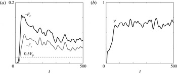
Figure 12 shows two different representations of the scalar flux at the interface. On the left-hand side, the curves for the sediment and salinity interfacial fluxes share an overall shape, having common peaks and valleys. Both scalar fluxes are driven by the instability at the interface, and so the similarity is expected. The ratio of the salinity to sediment scalar flux is shown in the plot on the right. We note that the flux ratio plateaus at an approximate value of 0.67, which is very similar to experimental measurements for double-diffusive thermohaline fingers (Turner Reference Turner1967; McDougall & Taylor Reference McDougall and Taylor1984).
(a) Interfacial scalar flux of sediment (black trace) and salinity (grey trace). The dotted line represents the interfacial sediment flux due to Stokes settling. (b) The interfacial flux ratio,
 ${\it\gamma}_{int}$
, oscillates about a quasi-steady value. Same parameters as figure 4.

An alternative way to measure the scalar flux is to calculate a turbulent diffusivity. We will evaluate the turbulent diffusivity at the interface, both because it is the region of the most interest and because the scalar mean fields have a non-zero gradient:
 $$\begin{eqnarray}K_{c}=\left.\frac{-F_{c}}{\text{d}\langle C\rangle /\text{d}z}\right|_{z=z_{c}}.\end{eqnarray}$$
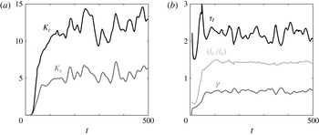
The left plot of figure 13 shows the turbulent diffusivities for both the sediment and salinity scalar fields. After the initial growth period, the values of the turbulent diffusivities begin to level off. Comparing the turbulent diffusivities to their molecular counterparts can provide context to the numbers seen in the plot. For the sediment field, this amounts to the calculation of the ratio
 $K_{c}/({\it\tau}\mathit{Sc})^{-1}$
which, if one averages the turbulent diffusivity from
 $100\leqslant t\leqslant 500$
, has a value of approximately 200. Thus, the instability has increased the effective diffusion of the sediment field by over two orders of magnitude. Performing the analogous calculation for the salinity field shows a fourfold increase over molecular diffusion alone. Comparing the two values, we can see that turbulent diffusion resulting from the instability has transformed sediment from diffusing 25 times more slowly than salinity, to diffusing twice as fast, a dramatic reversal.
(a) The turbulent scalar diffusivity for both sediment (black trace) and salinity (grey trace). (b) The turbulent diffusivity ratio (black trace), as well as the flux ratio
 ${\it\gamma}_{int}$
(dark grey trace) and the interface thickness ratio (light grey trace). Both of the diffusivities along with the flux ratio are calculated at the sediment interface. Same parameters as figure 4.

The figure indicates the presence of strong fluctuations in the signal for both turbulent diffusivities, which is consistent with the fluctuations shown in the interfacial fluxes. The idea that these fluctuations are an intrinsic property of the system will be discussed below. The fluctuations of the sediment and salinity fluxes are also strongly correlated. Similarly to the flux ratio
 ${\it\gamma}_{int}$
, the turbulent diffusivity ratio
 ${\it\tau}_{t}$
characterizes the relationship between the two turbulent diffusivities
 $$\begin{eqnarray}{\it\tau}_{t}=\frac{K_{c}}{K_{s}}=\frac{-F_{c}}{F_{s}}\frac{l_{c}}{l_{s}}=\frac{1}{{\it\gamma}_{int}}\frac{l_{c}}{l_{s}}.\end{eqnarray}$$
The right-hand side of figure 13 shows that the turbulent diffusivity ratio oscillates around a value that is slightly above two, again highlighting the fact the sediment is now diffusing faster than salinity. Equation (4.7) shows that the turbulent diffusivity ratio can be recast as the product of the interface thickness ratio with the inverse of the interfacial flux ratio. The figure also shows that all three of these reach quasi-steady values after the instability has fully developed.
A more application-oriented alternative to the interfacial sediment flux is to define an effective settling velocity. The effective settling velocity measures how fast the scalar settles due to enhancements caused by instabilities, as opposed to simply the Stokes settling velocity of a single grain. One such approach is to scale the horizontally averaged scalar flux by the horizontally averaged scalar field
 $$\begin{eqnarray}V_{p}^{enh}=\frac{-\langle w^{\prime }C^{\prime }\rangle }{\langle C\rangle }.\end{eqnarray}$$
Here, the minus sign reflects that the sediment is moving (settling) in the
 $-z$
direction. An analogous metric can be defined for salinity. Figure 14 shows the enhanced settling metric for both sediment and salinity, respectively. The value of the enhanced settling is over an order of magnitude greater than that of Stokes settling alone. As a note, care must be taken when interpreting this quantity, as it has in the denominator a term that is zero (or very small) in a large portion of the domain; the lower half for sediment and the upper for salinity. This issue is also related to the top/bottom asymmetry exhibited by both plots. One interpretation of this asymmetry is that even though the flux is quasi-symmetric (see figure 11), the enhanced settling is heavily dominated by the migration of mass into the deficient half of the domain; again, the lower half for sediment and the upper for salinity.
Time variation of the enhanced settling velocity for sediment (a) and salinity (b). Both fields show large regions with enhanced settling velocities of
 $O(1)$
, which is over an order of magnitude larger than the Stokes settling velocity of
 $V_{p}=0.04$
. Same parameters as figure 4.

4.2. Three-dimensional flow development
Up to this point, our analysis has focused on the dynamics of a representative two-dimensional flow field. However, it is important to establish the similarities and differences that occur with the addition of a third dimension. In this section, we analyse a representative three-dimensional flow field which has the same parameters as the previous two-dimensional flow except that the Schmidt number has increased from
 $\mathit{Sc}=0.7$
to
 $\mathit{Sc}=7$
. This change was made to highlight different flow features. In addition, compared with the flow shown in figure 4, the domain size has changed to
 $x,y\in [0,100)$
and
 $z\in [-110,65]$
while using a resolution of
 $N_{x}=N_{y}=512$
and
 $N_{z}=1537$
. As stated before, the remaining parameters are unchanged:
 $V_{p}=0.04$
,
 $R_{s}=2$
and
 ${\it\tau}=25$
.
4.2.1. Flow structure
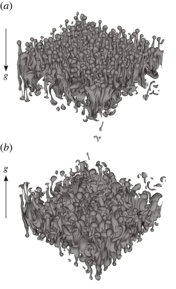
Shown in figure 15 are two views of the flow taken at time
 $t=100$
(the gravity vector has been included for orientation). Differences in the structure of the upward (a) and downward (b) moving fingers are just beginning to emerge at this time. The upward moving fingers are more regularly structured and oriented primarily in the vertical direction. In contrast, the downward moving fingers show disorder, a large degree of non-uniformity, as well as the merging of finger groups.
Contours of the sediment field showing (a) upward- and (b) downward-moving fingers. Contour value of
 $C=0.5$
taken at
 $t=100$
.

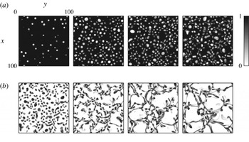
Figure 16 uses horizontal slices taken from
 $z=\pm 10$
to more clearly show the presence of both instability modes. The figure plots the sediment concentration above (a) and below (b) the interface at four different times. Above the interface, the plots are composed of quasi-circular light spots, which represent the upward moving fingers. The only change seen in this structure is the appearance of more fingers from the first to the second frame, otherwise the slices are difficult to distinguish. The first frame for the downward-moving fingers has a similar structure to the upward-moving fingers. It is also clear from comparing both frames at
 $t=75$
that the fingers move faster in the direction of settling, i.e. downward. At
 $t=100$
, the effects of the Rayleigh–Taylor mode can clearly be seen. The fingers (dark regions) are no longer mostly circular but are stretched by local convection zones, thereby attaining a more sheet-like structure. As time progresses, the convection zones (white areas) become larger and polygon-like in shape. This suggests that the thin finger structures themselves are created by the double-diffusive mode while the Rayleigh–Taylor mode results in the merging of these smaller structures into thin layers.
The sediment concentration taken from horizontal slices at
 $z=10$
(a) and
 $z=-10$
(b) for times
 $t=75$
(left), 100, 125, 150 (right).

4.2.2. Horizontally averaged quantities
Since much of the analysis in § 4.2 is based on the analysis of horizontally averaged profiles obtained from two- and three-dimensional simulations, it is important to understand how the dimensionality of the simulations affects these horizontally averaged profiles. This will enable us to appreciate the range of validity as well as the limitations of two-dimensional simulations, which have the advantage of being much less costly in time, effort or resources required.
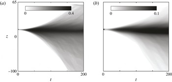
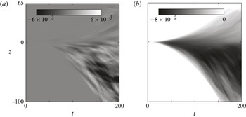
Figure 17 plots the r.m.s. fluctuations of the sediment (a) and salinity (b) fields. Even though the Schmidt number is different, these plots are overall quite similar to their two-dimensional counterparts in figure 6. There is a dark central region which represents the active fingering region. The growing dark envelope represents the growth of fingers and eventual release of plumes into the upper/lower layers of fluid. The sediment field is markedly more active in the fingering process as seen by the fourfold difference in the colourbar scales. All of these features are signatures of the instability irrespective of the domain being two- or three-dimensional. Also, the asymmetry of the upward- and downward-moving fingers is reflected in the shading of both profiles.
Time variation of three-dimensional, horizontally averaged sediment (a) and salinity (b) r.m.s. fluctuations.

A feature that is not present in figure 17 is the thin, streak-like structure seen in figure 6. In the two-dimensional flow, these streaks are prominent within the image and can have a large impact on the averaged profile even though they represent a rather local phenomenon. There could be two reasons why streaks no longer appear in the three-dimensional averaged profile; one, the plumes themselves are weaker; and/or two, the additional dimension has effectively averaged out the effects of any single plume. Based on the contours seen in figure 15, the instantaneous plume field looks similar in the two- and three-dimensional cases. On the other hand, adding an extra dimension severely reduces an individual plume’s impact, even accounting for the smaller horizontal extent in the three-dimensional simulations. As an example, the two-dimensional flow had an initial dominant wavenumber of
 $k_{dom}\approx 64$
, so that each plume occupies roughly
 $1/64$
th the horizontal extent. The three-dimensional simulation had a smaller dominant wavenumber of
 $k_{dom}\approx 16$
, so that a single plume occupies approximately
 $(1/16)^{2}=1/256$
th of the horizontal area. The important takeaway message is that three-dimensional flows will not be strongly affected by individual structures and thus will have a smoother average profile. As a result, all quantities derived from these average profiles will also be much smoother than their two-dimensional counterparts.
In figure 18, we see the horizontally averaged profiles for the horizontal and vertical scalar fluxes. Here, the horizontal flux is the average of the two horizontal directions, i.e.
 $0.5(\langle u^{\prime }C^{\prime }\rangle +\langle v^{\prime }C^{\prime }\rangle )$
. Again, the overall profiles are much smoother than their two-dimensional counterparts, while sharing the important features. There is a region of large horizontal flux in the lower half of the domain which is the result of plumes interacting with one another to create strong horizontal velocities. Looking past the similarities, there are also two important differences, due mainly to the change in Schmidt number. First, the largest vertical fluxes no longer occur at early times; instead, they occur throughout the late time region and are located below the fingering interface. The increase in the Schmidt number reduces the overall double-diffusive flux, which effectively makes the settling velocity of
 $V_{p}=0.04$
more dominant than in the case with
 $\mathit{Sc}=0.7$
. Thus, the vertical flux is largest below the interface due to the additional presence of the Rayleigh–Taylor instability.
The second noticeable difference are the thick, dark/light bands in both components of the flux. These bands are different from the streak structure seen in the two-dimensional case, which is related to plume release; they represent the merged finger groups created by the Rayleigh–Taylor mode. Focusing on the vertical flux in the region below the interface, there are slight striations in the shading for increasing time, which indicates a characteristic time associated with the Rayleigh–Taylor convection. This is consistent with the heuristic argument made at the end of § 4.1.1 regarding the boundary-layer-like dynamics of the unstable nose region.
Detailed comparisons between two- and three-dimensional simulations generally show an excess of structure in two dimensions as compared with three. On the other hand, global flow properties such as the growth rate of the interfacial thickness with time, the upward (downward) migration of the salinity (sediment) interfaces, and the associated scalar flux remain quantitatively similar. For additional information, we refer the reader to Burns (Reference Burns2013).
4.3. Fingering and leaking
One of our main motivations is to understand the two different instability types, leaking and fingering, seen in experiments by Parsons et al. (Reference Parsons, Bush and Syvitski2001). In Burns & Meiburg (Reference Burns and Meiburg2012), linear stability analysis was able to identify the ratio
 $H/l_{s}$
as the dominant parameter to determine if a system would be prone to fingering or leaking. In § 4.1.1, fully nonlinear DNS confirmed the importance of this ratio and attributed its quasi-steady value to the balance between the double-diffusive and settling fluxes. In § 4.2.1, we have also shown the appearance of Rayleigh–Taylor-like modes when this ratio becomes large. What remains is to answer the question of why leaking results from the interaction of double-diffusive and Rayleigh–Taylor modes.
Time variation of three-dimensional, horizontally averaged horizontal (a) and vertical (b) sediment scalar flux profiles.

To do so, we shift our focus from analysing vertical profiles, e.g.
 $\langle C^{\prime 2}\rangle (z,t)$
, to horizontal profiles, e.g.
 $C^{\prime }(x,z=z_{c},t)$
. Again, qualitative and quantitative tools will each play a role in understanding the behaviour of our system. Owing to periodicity in the horizontal directions, Fourier analysis will be the main quantitative tool and it will be used to obtain insight into both two- and three-dimensional flows.
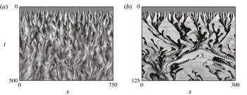
Figure 19 shows the time evolution of sediment fluctuations, contained in a horizontal slice at
 $z=0$
, for all times and both the fingering and leaking mode. In both cases, the data is extracted from two-dimensional simulations. The darker (lighter) colours represent heavy (light) fluctuations corresponding to the passing of negatively (positively) buoyant fingers through the horizontal plane. As a note, the pixelated nature of the images is due to low output resolution in time and is not a reflection of solution accuracy. Beginning with the fingering mode, the early time sees a much smaller dominant wavelength, before the secondary instability emerges and larger structures are created. Subsequently, the flow enters a state with no apparent structure to the location of fingers.
The time evolution of the sediment fluctuations taken from a horizontal slice at
 $z=0$
(no averaging). Shown are a fingering dominated mode (a) from the flow studied in § 4.1 and a leaking dominated mode (b). The key parameter values are
 $(\mathit{Sc},V_{p})=(0.7,0.04)$
and
 $(7.0,0.08)$
.

In stark contrast is the leaking mode, which clearly contains an organization amongst fingers. During early times no structures are observed, since the instability first develops at a moving interface front and would require a non-constant vertical location for the slice. When fingers do appear, they quickly merge together into five or six thin regions spread over the domain which then themselves merge into yet fewer regions. To achieve these merging events, the fingers themselves undergo strong horizontal motions at the interface, another characteristic observed in the experiments performed by Parsons et al. (Reference Parsons, Bush and Syvitski2001). Lastly, the heavy fluctuations in the leaking case are much darker than those of the fingering case which means that the fluctuations themselves are larger in the leaking case.
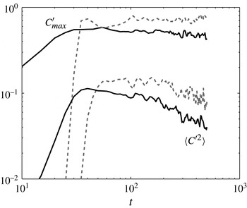
To quantify the differences seen between the two modes, figure 20 plots the maximum fluctuation,
 $C_{max}^{\prime }$
, and the r.m.s. value,
 $\langle C^{\prime 2}\rangle$
, for the profiles shown in figure 19. With regard to the maximum fluctuation, the fingering profile shows a slight decay over time and values in the range of 0.4–0.5, at later times. In contrast, the leaking case has peak values around 0.7–0.8 and remains steady. Fluctuations are heavier in the leaking case because the structures themselves are more isolated and thus heavier compared with the averaged fluid density. Partially due to their larger magnitude, the r.m.s. fluctuation is also greater for leaking than for fingering.
The instability mode can be distinguished using the maximum fluctuation size,
 $C_{max}^{\prime }$
, or the fluctuation r.m.s. value,
 $\langle C^{\prime 2}\rangle$
. Both metrics are shown for the fingering (solid black) and leaking (dashed grey) cases.

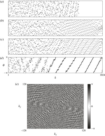
Next, we transform the fluctuations to Fourier space to look at the spectral power and the spectral phase shift. The power spectrum will reveal which scales contain energy. We hypothesize that the presence of the longer-wavelength Rayleigh–Taylor mode in the leaking instability leads to a vastly different power spectrum as compared with a double-diffusive case. The spectral phase shift holds information about the structure in the flow, although this is structure only in a global sense and not a local one.
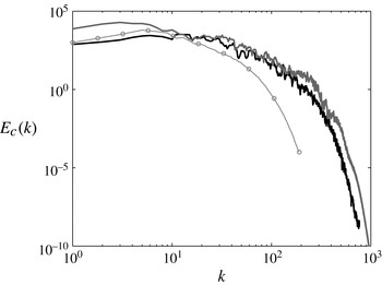
We start with the power spectrum of the sediment fluctuations in figure 21. This plot contains spectra from simulations of two-dimensional fingering (thick black trace), two-dimensional leaking (thick grey trace) and a three-dimensional intermediary (thin grey trace and circles). The overall shape of all three curves is very similar; being composed of a nearly constant energy plateau at low wavenumbers, followed by a slow decay in energy in the mid wavenumbers and ending with a strong drop in energy at the smallest scales. The spectra do not contain a turbulent inertial range with the well-known
 $-5/3$
rd slope. While the flows do exhibit a range of scales and a certain amount of disorder, they are not turbulent in the classical sense. One clear difference between the leaking and fingering spectra is the higher energy content at the very largest scales for the leaking case. This is consistent with the observation that the Rayleigh–Taylor modes observed in the flow field have a larger size than the fingering structures.
Energy spectra of sediment concentration for three different cases: two-dimensional fingering (thick black trace), two-dimensional leaking (thick grey trace) and a three-dimensional intermediary (thin grey trace,
 $\circ$
). The three-dimensional spectrum is calculated from a dataset of only every other grid point, thus the full simulation shows stronger decay at higher wavenumbers.

Phase locking is seen in both two- (a–d) and three-dimensional (e) simulations of leaking. The phase angle,
 ${\it\phi}$
, from a fingering simulation (a) is shown as a reference to compare against the phase locking seen at three different times of a single leaking simulation (b–d). In three dimensions, the striations in colour along the diagonals also indicate phase locking.

Figure 22 has two main parts; the top half displays the phase angle,
 ${\it\phi}$
, from two-dimensional simulations, while the bottom half is from a three-dimensional simulation. Starting with the two-dimensional simulations, the first frame (a) is a reference frame taken at time
 $t=400$
from a simulation with a clear fingering instability. There is no structure within the phase angle across the different wavenumbers, which is consistent with the observation that fingers develop uniformly across the entire interface, as seen in figure 19 and earlier in figure 4. As a note, frame (a) has no data after
 $k=768$
because it used less horizontal grid points than the subsequent leaking simulation, 1536 versus 2048. The phase angle becomes interesting for frames (b)–(d), taken from a leaking simulation at times
 $t=(125,250,375)$
at a constant
 $z$
-location. Here, the largest wavenumbers appear to phase lock, or align themselves on the interface and, as the flow progresses, this process moves to smaller and smaller wavenumbers. By frame (d), a structure has been established with the phase locking becoming dramatic;
 ${\it\phi}$
is basically a linear function of
 $k$
in a large wavenumber range. Physically, this means that the very small-wavelength modes align themselves in the flow to have a large impact despite no single mode containing very much energy. This superposition of modes is exactly what defines the leaking instability. The bottom image in figure 22 is an attempt to visualize phase alignment in a three-dimensional flow. Note that the colourmap used is circular, i.e. the same colour at both end points, in order to eliminate any false colour bands caused by the periodicity of the phase angle itself. Although difficult to see in black and white, there are visible high-frequency striations along both diagonals as well as a lower-frequency belt running almost horizontally across
 $k_{y}=0$
. Phase locking will always be more difficult to visualize in three dimensions, partly due to the visualization process and partly due to the vastly larger number of leaking configurations available with an extra dimension.
Thus, the leaking mode appears to be the result of phase locking that occurs when Rayleigh–Taylor modes interact with double-diffusive modes. The spectral content of both modes remains very similar, meaning the double-diffusive mode is constantly generating finger-like structures at the interface. However, these structures are quickly phase locked by the large-scale convection driven by Rayleigh–Taylor modes. Multiple small fingers merge together and are released out of the unstable nose layer in the form of thin, wisp-like plumes. The location of these thin plumes is constantly changing because of the periodic generation of Rayleigh–Taylor modes trying to balance the settling flux of sediment into the nose region; double-diffusion being insufficient to balance the flux alone.
5. Parametric study
From the above simulations, the following picture emerges: the key parameter that determines whether the settling process is dominated by double-diffusive or Rayleigh–Taylor instability is the ratio of the nose height
 $H$
over the salinity interface thickness
 $l_{s}$
. For small values of
 $H/l_{s}$
, the regions of strong salinity and sediment concentration gradients exhibit substantial overlap, and double-diffusive effects are prominent. Larger
 $H/l_{s}$
values lead to an increasing spatial separation of the salinity and sediment concentration gradients, so that double-diffusive mechanisms are suppressed. Instead, at the sediment interface an unstable density stratification evolves that gives rise to a Rayleigh–Taylor instability. We will now explore how the ratio
 $H/l_{s}$
is affected by the three main governing dimensionless groups
 $V_{p}$
,
 $\mathit{Sc}$
and
 $R_{s}$
. The above simulations for
 $\mathit{Sc}=0.7$
and
 $\mathit{Sc}=7$
already shed some light on the influence of the Schmidt number: for small
 $\mathit{Sc}$
values, strong molecular diffusion results in a wide salinity interface and renders
 $H/l_{s}$
sufficiently small for double diffusion to dominate. Larger
 $\mathit{Sc}$
values, on the other hand, result in a much sharper salinity interface and a correspondingly larger value of
 $H/l_{s}$
, so that the double-diffusive mode is suppressed and the Rayleigh–Taylor mode takes over. In order to identify the proper scaling relationships for this
 $\mathit{Sc}$
effect, and to quantify the influence of
 $V_{p}$
and
 $R_{s}$
on
 $H/l_{s}$
, we now conduct a parametric study, based on ensemble-averaged, two-dimensional simulations.
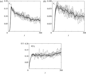
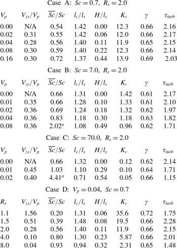
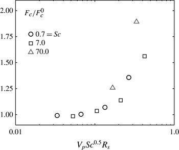
As part of the parametric study, we ran 10 simulations with different random initial perturbations for each of the 17 parameter combinations shown in table 1, for a total of 170 simulations. Cases A–C focus on the role of the settling velocity for three different values of the Schmidt number, while case D varies the stability ratio for constant Schmidt number and settling velocity. We calculate statistical measures such as
 $z_{s}$
,
 $z_{c}$
,
 $l_{s}$
,
 $l_{c}$
,
 $F_{s}$
,
 $F_{c}$
, etc. for each simulation separately, and then average these statistics to find the ensemble average. As an example, figure 23 shows the time-dependent interfacial fluxes and the thickness ratio
 $H/l_{s}$
for case A with
 $V_{p}=0.04$
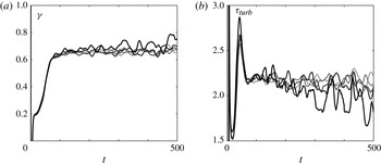
, which is the flow discussed in § 4.1. Individual simulations are plotted as thin grey lines, with the ensemble average indicated by a thick black line. Once averaged, the decay of the interfacial flux as a result of the thickening interface is clearly visible. The thickness ratio shows a well-defined plateau once the instability has become fully developed. The slight uptick towards the end of the simulation time is the result of a large plume beginning to interact with the bottom boundary.
The interfacial fluxes (a,b) and the thickness ratio (c) for case A with
 $V_{p}=0.04$
(the flow discussed in § 4.1). The ensemble-averaged statistics (thick black lines) are much smoother than those representing individual realizations (thin grey lines).

5.1. Interface region
Rather than describing the development of the interfacial region in terms of the four unsteady quantities
 $z_{c}$
,
 $z_{s}$
,
 $l_{c}$
and
 $l_{s}$
, we now rescale these variables in order to obtain four corresponding quantities that reach approximately steady values
 $$\begin{eqnarray}\displaystyle & \displaystyle V_{zs}=\frac{\text{d}z_{s}}{\text{d}t} & \displaystyle\end{eqnarray}$$
 $$\begin{eqnarray}\displaystyle & \displaystyle \overline{\mathit{Sc}}=\frac{4t}{l_{s}^{2}} & \displaystyle\end{eqnarray}$$
 $$\begin{eqnarray}\displaystyle & \displaystyle R_{t}=\frac{z_{s}-z_{c}}{l_{s}} & \displaystyle\end{eqnarray}$$
 $$\begin{eqnarray}\displaystyle & \displaystyle {\it\xi}=\frac{l_{c}}{l_{s}}, & \displaystyle\end{eqnarray}$$
 $\overline{\mathit{Sc}}$
represents the inverse of the diffusion coefficient for the horizontally averaged salinity, i.e. we assume that the mean salinity follows a diffusion equation:
 $\partial \langle S\rangle /\partial t=(1/\overline{\mathit{Sc}})(\partial ^{2}\langle S\rangle /\partial z^{2})$
. While the assumption of a constant upward interface velocity
 $V_{zs}$
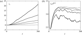
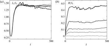
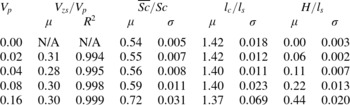
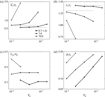
represents a good approximation for all settling velocities, the other three quantities become increasingly unsteady for higher settling velocities. We note, however, that their variation typically remains less than 15 %, which is quite small when compared with that of the unscaled variables. For increasing settling velocities, we note that the salinity interface sharpens and moves upward more rapidly. At the same time, the ratio
 $l_{c}/l_{s}$
decreases, which indicates that the sediment interface sharpens even more strongly than the salinity interface. The nose height is seen to increase for larger settling velocities.
The salinity interface location (a) and the salinity interface thickness (b) for the five different settling velocities of case A from table 1. Increases in the settling velocity are shown as darker curves.

The dimensionless group values and the grid properties for the parameter study fall into four larger classes. This table represents 17 distinct parameter combinations and a total of 170 separate realizations.

The interface thickness ratio (a) and interface nose thickness (b) for the five different settling velocities of case A from table 1.

In table 2 we summarize the above quasi-steady measures of the interface in terms of a mean value as well as an error measure. For the salinity position the error measure is the
 $R^{2}$
value from fitting
 $z_{s}(t-t_{0})=V_{zs}t$
, where
 $t_{0}$
represents the delay before the salinity interface begins to move upwards (see figure 24). For the remaining three quantities, we choose the standard deviation
 ${\it\sigma}$
as an appropriate error. Table 2 clearly shows that the largest settling velocity has the least stationary statistics, which is consistent with figures 24 and 25. The variation of the mean values with the Stokes settling velocity will be discussed below.
The ensemble-averaged interface described by four statistically stationary ratios for case A from table 1. Here,
 ${\it\mu}$
and
 ${\it\sigma}$
refer to the mean and standard deviation while
 $R^{2}$
is a measure of the linear fit to
 $z_{s}$
with slope
 $V_{zs}$
.

5.2. Scalar fluxes
Most of the quantities describing the scalar fluxes already develop semi-stationary statistics. These quantities are the turbulent diffusivity,
 $K_{c}$
, the turbulent flux ratio,
 ${\it\gamma}=-F_{s}/F_{c}$
, and the turbulent diffusivity ratio,
 ${\it\tau}_{turb}=K_{c}/K_{s}$
. Here,
 ${\it\gamma}$
and
 ${\it\tau}_{turb}$
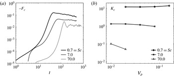
represent different ways of recasting the turbulent salinity flux in terms of the sediment flux. For reasons associated with the physical interpretation of the simulation results, we choose to retain both of these quantities.
Figure 26 examines the interfacial sediment flux both directly (a) and in the form of a turbulent flux coefficient (b). We note a sizeable increase in the flux for the largest settling velocity, where the leaking mode dominates. On the other hand, the corresponding increase in the turbulent diffusivity for the largest settling velocity is relatively mild, so that it cannot account for all of this flux increase. This suggests that the sediment concentration gradient in the mean flow must increase as well for the largest settling velocities, which is consistent with our observations in figures 24 and 25, and is also confirmed by table 2. We furthermore note that for the largest settling velocities the turbulent diffusivity displays strong temporal oscillations in the plateau region, which is typical of the leaking mode. In summary, we find that for large settling velocities the Rayleigh–Taylor-like overturning convection associated with the leaking mode both sharpens the sediment interface and periodically increases the magnitude of the scalar flux during the depletion of the nose region. Together, these two effects account for the increase in the flux for the largest settling velocities.


Figure 27 shows two alternative ways of quantifying the turbulent salinity flux; the flux ratio
 ${\it\gamma}=-F_{s}/F_{c}$
and the turbulent diffusivity ratio
 ${\it\tau}_{turb}=K_{c}/K_{s}$
. Similar to the sediment flux, these quantities change only at the highest settling velocities, i.e. in the presence of the leaking mode. Under those conditions the mean value of the flux ratio increases and it exhibits strong oscillations. The increase in the flux ratio reflects the enhanced salinity flux due to the convective overturning of the nose region associated with the leaking mode. This increase in the salinity flux manifests itself as a decrease in the turbulent diffusivity ratio, shown in the right frame of figure 27.
The flux ratio
 ${\it\gamma}$
(a) and the turbulent diffusivity ratio
 ${\it\tau}_{turb}$
(b). Same data sets and curve meanings as figure 26.

5.3. Scaling relationships
In order to obtain scaling laws for the above processes, we have to analyse their quantitative dependence on the governing parameters
 $V_{p}$
,
 $\mathit{Sc}$
and
 $R_{s}$
. This analysis will be based on the data in table 3, which provides ensemble-averaged values for the statistical quantities discussed in §§ 5.1 and 5.2, for all 17 parameter combinations. Sections 5.3.1 and 5.3.2 will separately discuss the influence of the settling velocity
 $V_{p}$
and the stability ratio
 $R_{s}$
on these statistical quantities, while § 5.3.3 will present a comprehensive picture that accounts for the combined influence of
 $V_{p}$
,
 $R_{s}$
and
 $\mathit{Sc}$
.
The mean value for the 17 (semi-)stationary statistics from each ensemble in the four different case studies. The a refers to simulations with strong leaking, which results in sharper interfaces and thus
 $\overline{\mathit{Sc}}>\mathit{Sc}$
.

5.3.1. Influence of the settling velocity
Figure 28 quantifies the statistical interface measures for cases A–C. Figure 28(a) shows that for the traditional double-diffusive fingering case, i.e. for vanishing settling velocity,
 $\overline{\mathit{Sc}}<\mathit{Sc}$
for all but the largest
 $\mathit{Sc}$
values. Hence, the diffusivity of the mean salinity profile is somewhat larger than that of the instantaneous salinity profile, which reflects the fact that the fingering process acts to diffuse salinity faster than molecular diffusion alone. For larger settling velocities
 $\overline{\mathit{Sc}}/\mathit{Sc}$
increases and can in fact reach values larger than one. This indicates that the diffusivity of the mean salinity profile drops below the molecular diffusivity. As a result, the mean salinity interface is sharper than what would be observed for an unperturbed salinity interface spreading due to molecular diffusion alone. This is consistent with our earlier findings, and it reflects the action of the overturning Rayleigh–Taylor structures. Figure 28(b) shows that for increasing settling velocities the sediment interface sharpens even more quickly than the salinity interface, so that the ratio
 $l_{c}/l_{s}$
decreases.
The ensemble average behaviour for the interface statistics from cases A–C, which all have
 $R_{s}=2$
. The dashed lines show the respective
 $V_{p}=0$
behaviour. The strong changes for
 $\mathit{Sc}=70$
are a consequence of a pronounced leaking instability.

The figure 28(c) indicates that the upward velocity of the salinity interface scales approximately with the settling velocity, so that
 $V_{zs}/V_{p}$
remains nearly constant. On the other hand, the ratio of the upward salinity interface velocity to the settling velocity varies appreciably with the Schmidt number.
In figure 28(d), we see that the thickness ratio
 $H/l_{s}$
depends strongly on both the settling velocity and the Schmidt number. The limited number of data points suggest a power-law relationship between the thickness ratio and the settling velocity for
 $\mathit{Sc}=0.7$
and
 $\mathit{Sc}=7$
. We will revisit the proper scaling for this curve below, after discussing the influence of the stability ratio.
Figure 29 analyses the behaviour of the interfacial sediment flux for a constant settling velocity (a), and for all ensembles in cases A–C (b). In the left frame, the double-diffusion-dominated low-
 $\mathit{Sc}$
case displays significantly higher interfacial flux than the leaking-dominated high-
 $\mathit{Sc}$
case. Furthermore, the double-diffusive instability develops on a much faster time scale, whereas the Rayleigh–Taylor mode sets in somewhat later, due to the time required for the unstable nose region to emerge. The Rayleigh–Taylor mode also displays the strongest oscillations, consistent with our earlier observations. The right frame indicates that the turbulent sediment diffusivity scales with the inverse of the Schmidt number, while its dependence on the settling velocity is quite small. When combined with our earlier observation in figure 26, which showed that the sediment flux depends only weakly on
 $V_{p}$
, this suggests that the sediment flux out of a river plume is primarily determined by the effects of diffusion, i.e. by the double-diffusive flux, rather than by the Stokes settling velocity.
The interfacial flux (a) for
 $V_{p}=0.02$
and
 $R_{s}=2.0$
, for three different Schmidt numbers. The turbulent diffusivity (b) for cases A–C shows a strong dependence on the Schmidt number and only a weak one on the settling velocity.

Figure 30 plots the ratio of the interfacial flux to the purely double-diffusive flux, i.e. the flux for
 $V_{p}=0$
. Even for the largest settling velocity, the flux only sees an average increase of approximately 56 % and a maximum increase near 100 %. While this represents an important effect, it is still small compared to that of the Schmidt number, which can change the interfacial sediment flux by an order of magnitude or more.
The interfacial flux,
 $F_{c}$
, for five different settling velocities scaled by the flux for pure double diffusion,
 $F_{c}^{dd}$
, i.e. for
 $V_{p}=0$
. Results for
 $\mathit{Sc}=7$
and
 $R_{s}=2$
.

5.3.2. Influence of the stability ratio
Much of the discussion so far has focused on the Schmidt number as a driver behind the double-diffusive character of a system. However, as seen in table 3, the stability ratio can play a similarly important role, with values of
 $R_{s}$
close to one causing a strong increase in the double-diffusive flux.
Figure 31 displays the interfacial flux for each ensemble from case D, as well as the associated turbulent diffusivity. We observe a strong decrease in the flux accompanied by an increase in the time scale. The turbulent diffusivity exhibits a power-law dependence on the stability ratio, with a slope close to negative one. This trend is mirrored in the values of
 $V_{zs}$
,
 $\overline{\mathit{Sc}}$
and
 $H/l_{s}$
shown in table 3. The decrease in the flux for increasing stability ratios reduces the upward velocity of the salinity interface while increasing the nose thickness ratio. The low
 $\overline{\mathit{Sc}}$
values, i.e. high salinity diffusivities, for small stability ratios are a consequence of the enhanced mixing in this parameter regime.
The interfacial flux (a) for
 $V_{p}=0.04$
and
 $\mathit{Sc}=0.7$
for five different stability ratios. The turbulent diffusivity (b) for case D shows a strong dependence on the stability ratio with a power-law exponent of approximately negative one.

5.3.3. The thickness ratio
Figure 32 shows the nose thickness ratio for all 14 ensembles that have non-vanishing settling velocities. Here, we have chosen the independent variable such as to collapse the data onto a straight line. As we will see in the following, this graph can be interpreted in terms of a balance between the inflow of sediment into the nose region from above, and the outflow of sediment from the nose region below.
The value of the nose thickness ratio,
 $H/l_{s}$
, can be predicted a priori based on the three main dimensionless groups. The dashed line shown has a slope of one.

The rate at which sediment enters the nose region from above, i.e. across the salinity interface, is determined both by the downward settling velocity
 $V_{p}$
, as well as by the upward velocity
 $V_{zs}$
of the salinity interface. Figure 28 had established that
 $V_{zs}\sim V_{p}$
, so that the overall rate at which sediment enters into the nose region from above is proportional to
 $V_{p}$
. The rate at which sediment leaves the nose region across its lower boundary, i.e. across the sediment interface, is given by the product of the turbulent sediment diffusivity
 $K_{c}$
and the sediment concentration gradient at the sediment interface
 $l_{c}^{-1}$
. Table 3 along with figures 29 and 31 shows that
 $K_{c}\sim (\mathit{Sc}R_{s})^{-1}$
. Furthermore,
 $l_{c}\sim l_{s}\sim \mathit{Sc}^{-0.5}$
, so that the overall rate at which sediment leaves the nose region below scales with
 $1/(\mathit{Sc}^{0.5}R_{s})$
. Consequently, the independent variable
 $V_{p}\mathit{Sc}^{0.5}R_{s}$
in figure 32 is proportional to the ratio of sediment flow into the nose region from above to sediment flow out of the nose region below. The collapse of the simulation data along a straight line with a slope of one thus indicates that the quasi-steady value that emerges for the scaled nose height
 $H/l_{s}$
is proportional to the ratio between inflow and outflow of sediment into the nose region. In other words, if the rates of inflow and outflow of sediment into the nose region are similar in magnitude, the amount of sediment contained in the nose region increases very slowly and
 $H/l_{s}$
remains small. On the other hand, if the rate of sediment inflow significantly exceeds the rate of sediment outflow, then sediment accumulates more rapidly in the nose region, thereby resulting in larger values of the scaled nose height
 $H/l_{s}$
. This demonstrates that the dynamics of the nose region, and hence of the entire settling process, is governed by the balance of the sediment fluxes into and out of the nose region.
Figure 33 displays the interfacial sediment flux, normalized by its double-diffusive value for vanishing Stokes settling velocity, as a function of the same dimensionless grouping
 $V_{p}\mathit{Sc}^{0.5}R_{s}$
. The plateau region for
 $V_{p}\mathit{Sc}^{0.5}R_{s}\leqslant O(0.1)$
confirms that for
 $H/l_{s}\leqslant O(0.1)$
the sedimentation process is governed by a classical double-diffusive instability. The strong increase in the sediment flux for
 $V_{p}\mathit{Sc}^{0.5}R_{s}\geqslant O(0.1)$
, on the other hand, reflects the shift from the double-diffusive to the leaking mode as
 $H/l_{s}\geqslant O(0.1)$
. In conclusion, the following picture emerges: for small values of
 $V_{p}\mathit{Sc}^{0.5}R_{s}$
, the sediment inflow into the nose region from above is small, and regular double-diffusive fingering at the sediment interface suffices to set up an approximately equal sediment outflow from the nose region. Hence, there is little sediment accumulation within the nose region, and
 $H/l_{s}$
remains small. As
 $V_{p}\mathit{Sc}^{0.5}R_{s}$
increases, i.e. as the ratio of sediment inflow to outflow increases, sediment accumulates in the nose region and
 $H/l_{s}$
grows. Beyond
 $H/l_{s}\approx O(0.1)$
, the Rayleigh–Taylor mode kicks in and enhances the sediment outflow beyond its purely double-diffusive value, thereby establishing a qualitatively different balance between in- and outflow.
The mean increase in the interfacial flux plotted against the scaling which collapses the nose thickness ratio. A sharp rise in the flux increase is seen when the instability type transitions to the leaking mode.

6. Summary and conclusions
We have employed DNS to analyse the rich dynamics of the instability mechanisms involved in the sedimentation of particles from buoyant river plumes. Our primary objective has been to understand the different stages of flow development for the double-diffusive fingering and leaking modes, to gain insight into the mechanisms governing the effective particle settling velocity, and to obtain scaling relationships for the above processes via a parametric study.
Our analysis of the DNS results focused on the evolution of horizontally averaged profiles. Averaging over the horizontal directions enables us to describe the flow field via just a handful of parameters. We define the ‘average’ sediment (salinity) interface as the location where the horizontally averaged sediment (salinity) field reaches a value of half its maximum, i.e.
 $\langle C\rangle =0.5$
. This interfacial region can then be described by four main parameters, namely a thickness and position each for the sediment and salinity fields.
The DNS results demonstrate that the salinity interface moves upwards, away from the downward-moving sediment interface, thereby forming a nose region in between these two interfaces. This vertical separation between the salinity and sediment interfaces is generated and maintained by the Stokes settling velocity, which creates a salinity imbalance between upward- and downward-moving fingers that causes the upward motion of the salinity interface. The scaled thickness of the nose region
 $R_{t}=H/l_{s}$
reaches a quasi-steady-state value once the flow is fully developed, i.e. when a balance is established between the flow of sediment into the nose region from above, the outflow of sediment from the nose region below and the rate at which sediment accumulates in the nose region. The scaled nose height
 $H/l_{s}$
represents the main parameter that determines whether the settling process is dominated by double-diffusive or Rayleigh–Taylor instability. Small values of
 $H/l_{s}\leqslant O(0.1)$
are characterized by double-diffusive settling, whereas at
 $H/l_{s}\geqslant O(0.1)$
Rayleigh–Taylor overturning of the nose region is observed. The parametric study and accompanying scaling analysis demonstrate that
 $H/l_{s}$
is a linear function of the single dimensionless grouping
 $V_{p}\mathit{Sc}^{0.5}R_{s}$
, which represents the ratio of inflow and outflow of sediment into the nose region. The simulation results furthermore indicate that double-diffusive and Rayleigh–Taylor instability mechanisms cause the effective settling velocity of the sediment to scale with the overall buoyancy velocity of the system, which can be orders of magnitude larger than the Stokes settling velocity.
We furthermore employ the tools of spectral analysis to study the formation of the leaking mode. The power spectra of the sediment fluctuations reveal no qualitative difference in the spectral content between the fingering and leaking modes. In both cases, there is a large contribution from wavelengths ranging in size from the largest in the domain to the most unstable mode predicted from linear stability, followed by a sharp decay in the spectral energy. This decay does not show the
 $-5/3$
rd slope typical of turbulent flows. Even though it is not evident from the power spectra, the difference between flows dominated by fingering and leaking is clearly seen when analysing the spectral phase shift. For leaking-dominated flows a phase-locking mechanism is observed, which intensifies with time. The leaking mode can be interpreted as a fingering mode which has become phase-locked due to large-scale overturning events in the nose region as a result of a Rayleigh–Taylor instability. The spectral content of fingering-dominated flow is preserved for leaking-dominated flow, since even for the leaking mode, the fingers are always generated at the double-diffusive scale but are then aligned by the Rayleigh–Taylor mode.
On a final note, the authors acknowledge that this work has reduced the complexity of the true problem of sedimentation from river plumes in order to draw meaningful conclusions about the specific problem of double-diffusion in the presence of settling. There are many ways to extend the current analysis to more realistically approximate a river plume. One possible extension is the addition of the shear layer generated by the river outflow. The pioneering work on double diffusion in a shear layer was performed by Smyth & Kimura (Reference Smyth and Kimura2007, Reference Smyth and Kimura2011), but this did not include particles. They show that for thermohaline double-diffusive shear layers, both salt sheets and Kelvin–Helmholtz instabilities can develop. Depending on the strength of the shear and the stability ratio, either shear or fingering can drive the resulting turbulent flow. The authors comment that for cases dominated by salt sheets, the density layer narrows with time. Based on our simulation results for double-diffusion with particles, we do not expect that observation to hold in salt–sediment systems. Nevertheless, we speculate that even in salt–sediment systems Holmboe instabilities may evolve in the presence of shear. Smyth and Kimura furthermore observe that shear reduces mixing in thermohaline systems, even though it provides an additional energy source. It will be interesting to explore whether similar findings will be observed for salt–sediment systems.
A second interesting extension would be the addition of an improved particle settling model. The works by Aliseda et al. (Reference Aliseda, Cartellier, Hainaux and Lasheras2002) and Bosse, Kleiser & Meiburg (Reference Bosse, Kleiser and Meiburg2006) on inertial particles and turbulence-induced clustering provide a good reference on possible effects. Lastly, it will be interesting to explore how the emerging picture of thermohaline double diffusion regarding secondary instabilities, horizontal intrusions and staircase formation (Stellmach et al. Reference Stellmach, Traxler, Garaud, Brummell and Radko2011; Traxler et al. Reference Traxler, Stellmach, Garaud, Radko and Brummell2011) changes when one of the species has a settling velocity.
Acknowledgements
The authors dedicate this article to the memory of Professor T. Maxworthy, whose early, groundbreaking experiments on double-diffusive sedimentation partly inspired this investigation. We furthermore acknowledge R. Henniger and L. Kleiser for the use of the code IMPACT used to simulate the three-dimensional flows and P. Garaud and T. Hsu for helpful discussions. P.B. especially thanks P. Schmid for an insightful discussion which added a great deal to this work. This work would not be possible without computing time on the CU-CSDMS High-Performance Computing Cluster and the Janus supercomputer, which is supported by the National Science Foundation (award number CNS-0821794) and the University of Colorado Boulder. The Janus supercomputer is a joint effort of the University of Colorado Boulder, the University of Colorado Denver and the National Center for Atmospheric Research. This work was supported through NSF grants CBET-0854338, CBET-1067847, OCE-1061300 and CBET-1438052.