INTRODUCTION
Global population growth, increase in per capita consumption, changing governance of global food systems, climate change, competition for key resources and changes in consumer preferences are considered as the key drivers of change affecting the food system in the years ahead (Foresight 2011). These factors, coupled with policy changes such as Common Agricultural Policy (CAP) reforms, increase the economic and social pressure on many breeding beef suckler cattle farms (Vosough Ahmadi et al. Reference Vosough Ahmadi, Shrestha, Thomson, Barnes and Stott2015a ). The challenge is particularly important in Scotland and similar high-quality/low-volume specialist systems in other EU member states with a good reputation for producing quality beef from extensive grass-based systems in remote and often environmentally sensitive areas. Management of breeding beef suckler herds in these systems requires a difficult but vitally important balance between often conflicting needs for farm profits, animal health and welfare and sustainable food production.
Trade-offs arise in various aspects of farming and animal husbandry, including feeding, reproduction, health, welfare and marketing. For example, Drennan & Berry (Reference Drennan and Berry2006) reported that spring-calving cows (calving early in the year) had significantly higher weight at the start of winter and greater body condition score (BCS) at the subsequent calving, but lost most live weight in the subsequent winter. Parity, lower weight gain and BCS can affect the frequency of calving difficulty (Drennan & Berry Reference Drennan and Berry2006). These factors could also affect animal welfare, incidence of diseases or the involuntary culling rate. Cow body weight, body condition at calving and gestation length, along with non-genetic factors such as age and parity, year and season of calving, place of calving, maintenance practises, diseases, calf sex and nutrition influence the frequency of calving difficulty (Zaborski et al. Reference Zaborski, Grzesiak, Szatkowska, Dybus, Muszynska and Jedrzejczak2009). The frequency of calving difficulty and involuntary and voluntary culling rates that may represent the parity and age of the animals are therefore considered as indicators of animal welfare in suckler herds. High BCS reflects a good level of general health, nutrition and fertility management of the animals (Frasier & Pfeiffer Reference Frasier and Pfeiffer1994; Drennan & Berry Reference Drennan and Berry2006), but high BCS may increase the chance of calving difficulties particularly in breeds and crosses with relatively small pelvic canals such as Friesian in relation to their mature size (Lowman Reference Lowman1988) and could affect the probability and the timing of conceptions.
Reproduction management is an important factor affecting profitability of suckler herds. Barbudo et al. (Reference Barbudo, Gunn and Stott2008) reported that the profitability of the herd increases as the length of calving period shortens and early conception rate, hence early calving, increases. This may require culling of late-calving animals and barren cows, and replacing them with heifers. This will change the age structure of the herd and impose extra financial costs such as variable costs of feeding and management that are required for the replacement heifers, as well as further fixed costs. This is particularly the case in winter when grazing on pasture and feed are limited. Changed culling policy and age structure of the herd may also affect animal welfare as a result of higher frequency of calving difficulty. In addition, the culling and replacement decision is also influenced by price determinants such as weight and BCS of cows as well as market prices, which affect the cost of replacing cows and rearing heifers. Understanding the potential interactions between these elements and possible trade-offs between fertility, animal welfare and profitability of breeding suckler cattle requires methodologies that could encompass at least some elements of the crucial aspects of this farming system. However, understanding depends on capturing the long-term (between production cycles) as well as the short-term (within production cycle) impacts of key decisions and events that govern these interactions and hence the performance of beef suckler herds.
Dynamic programming (DP) modelling has the potential to incorporate repetitive managerial decision options and related stochastic events, identifying the series of decisions that maximize the expected net present value of current and future animals in herds given bio-physical inputs and assumptions. In the past, applications of DP models in cattle farming have been confined mainly to dairy farming systems (Van Arendonk Reference Van Arendonk, Korver and van Arendonk1988; Kennedy & Stott Reference Kennedy and Stott1993; Stott et al. Reference Stott, Jones, Gunn, Chase-Topping, Humphry, Richardson and Logue2002, Reference Stott, Jones, Humphry and Gunn2005; Bar et al. Reference Bar, Tauer, Bennett, González, Hertl, Schulte, Schukken, Welcome and Gröhn2008; Cha et al. Reference Cha, Hertl, Bar and Gröhn2010, Reference Cha, Bar, Hertl, Tauer, Bennett, González, Schukken, Welcome and Gröhn2011), perhaps because the detailed data required for these models are more accessible in dairy than in beef suckler herds. However, DP models have also been used in determining optimal replacement and management policies in beef cows (Frasier & Pfeiffer Reference Frasier and Pfeiffer1994). Replacement decisions, among many other crucial factors, affect the economics, health, fertility, welfare and environmental footprint of breeding suckler herds. For example, higher replacement rates require more breeding animals to provide replacement heifers rather than productive beef calves, therefore increasing the environmental impacts of the business, i.e. greenhouse gas emissions and soil degradation per unit of output. Applications of optimization models in suckler cattle that seek improved management strategies by evaluating the potential interactions and trade-offs between different components of these farming systems are limited in the current literature. In the current study, this deficiency was addressed by using a DP model that was parameterized by farm performance data and with the objective of assessing the possible mentioned trade-offs. Five-year performance data obtained from a closely monitored beef suckler cattle farm was analysed and meaningful relationships between BCS and parity with other variables of interest, i.e. calving period, incidences of involuntary calving and calving difficulty scores (CDSs), were evaluated. The estimates of transition probabilities between the states of cattle, probability of involuntary culling and probability of calving difficulty were subsequently incorporated to parameterize a plausible DP model. The application of an optimization DP model in assessing the trade-offs between indicators of performance (e.g. calving rate and weight gain) and indicators of sustainability (e.g. animal welfare and replacement rate) in breeding beef suckler cattle farms by using farm performance data is considered as the novelty value of the current study. Body condition score was used in the DP model as an indicator of animal welfare that reflects feeding and nutritional conditions of the animals. It should be noted that the overall animal welfare score of given farms or animals could only be captured by assessing and taking into account five freedoms (FAWC 2001) and/or by considering Welfare Quality protocols (Blokhuis et al. Reference Blokhuis, Veissier, Miele and Jones2010).
MATERIALS AND METHODS
Data
Data were collected from Scotland's Rural College's (SRUC) Beef farm at Easter Howgate for a period of 5 years (2006–10). The herd consists of 200 suckler cows. Replacement heifers were homebred, with Limousin (LIM) and Aberdeen Angus (AA) breeds used for their suitability as sires of replacement heifers. Belgian Blue (BB), Simmental (SIM) and Charolais (CH) were also used as terminal sires (i.e. purebred sires that are used to breed crossbred dams). All the mentioned breeds were included under one categorical variable in the statistical models. Cows were bred by artificial insemination (AI) with triple synchronization of oestrus to calve during March and May. Three main AI services for the whole herd took place on 20 June, 15 July and 7 August of every year. As a result it was expected that calving would start around mid-March and extended to early May. Three calving periods corresponding to AIs were therefore considered, but as calving incidents happened until the end of May, a fourth calving period was added. The calves were weaned in October and housed. The cows were housed at weaning and fed a straw-based diet through the winter. Finished animals were sold mainly to local abattoirs at 12–14 months of age.
Data included information on individual breeding suckler cows, including breed, parity, calving period, CDS, body weights, BCS at weaning, number of services received and involuntary culling status. A cow was identified as barren if it did not conceive after receiving three services. The CDS of a cow was measured on an ordinal scale (1 = no assistance; 2 = assisted by stockman; 3 = use of calving jack or calved by veterinarian performing caesarean; 4 = calf died during calving). Body condition score is determined on a scale of 1 (thin, poor) to 5 (obese, grossly fat) (Drennan & Berry Reference Drennan and Berry2006). In the current data set, the BCS of cows actually ranged from 2 to 4 on this 1–5 scale. For practical purposes, BCS was categorized at three levels: low (BCS < 2·50), middle (2·50 ⩽ BCS ⩽ 3·25) and high (BCS > 3·25). These are consistent with moderate/poor, good and fat/grossly fat categories respectively, suggested by DEFRA (DEFRA 2000). Parity was categorized by ten levels with parity ten or more combined together since few cows with more than ten parities were recorded (28 out of 928 records). Finally, the categorical variable breed was considered at three levels: AAX (Aberdeen Angus and its crosses), CH & CHX (Charolais and its crosses) and other (Limousin, Simmental and other crosses).
Statistical models
Appropriate statistical models were developed for the data on the incidence of involuntary culling, CDS and frequencies of different calving periods (response variables). All models included parity as an explanatory variable (to integrate with the DP model as discussed later); breed and BCS were also candidate explanatory variables and their final inclusions in the model was based on their statistical significance (P < 0·10). All models initially included cow as a random effect, but due to very low estimates of between cow variability, final models excluded the cow effect. The final fitted models were subsequently used to parameterize the DP model discussed later. All statistical analyses were carried out using R software version 3.1·0 with appropriate R packages (stats, lme4, MASS, ordinal) (R Core Team 2014).
Incidence of involuntary culling
Involuntary culling was defined as an incident recorded in the data set where a breeding cow was involuntarily culled because of the occurrence of diseases such as Johne's disease, injuries and/or poor health. The incidence of involuntary culling for the ith observation (y
i
) is assumed to follow a Bernoulli distribution with probability φ
i
, and modelled by a generalized linear model (GLM) with a logit link function. The fitted GLM is:
 ${\rm logit}(\phi _i) = \sum\nolimits_{k = 1}^{10} {\beta _kp_{ik}} $
, where p
ik
is 1 if the parity of the ith cow is k and 0 otherwise, and β
k
represents the coefficient for the kth parity. The fitted GLM was used to obtain the estimated probabilities of involuntary culling at each level of parity.
Calving difficulty score
The CDS of the ith observation (y
i
) was assumed to follow a multinomial distribution with parameters {φ
ij
}, where φ
ij
denotes the probability that the ith observation falls in the jth category of the CDS; j = 1,…, 4, representing four ordinal levels of CDS where increasing order of j suggests increasing calving difficulty. The data on y
i
were modelled using a cumulative link model (CLM) where the cumulative probabilities are defined as: ψ
ij
= P(y
i
⩽ j) = φ
i1 + · · · + φ
ij
. The fitted CLM with a logit link function is:
 ${\rm logit}(\psi _{ij}) = \theta _j - \left( {\sum\nolimits_{k = 1}^{10} {\beta _kp_{ik}} + \sum\nolimits_{m = 1}^3 {\omega _mb_{im}}} \right)$
, where p
ik
is 1 if the parity of the ith observation is k and 0 otherwise, b
im
is 1 if the breed of the ith observation is m and 0 otherwise, θ
j
is the intercept for the jth category of the CDS; β
k
and ω
m
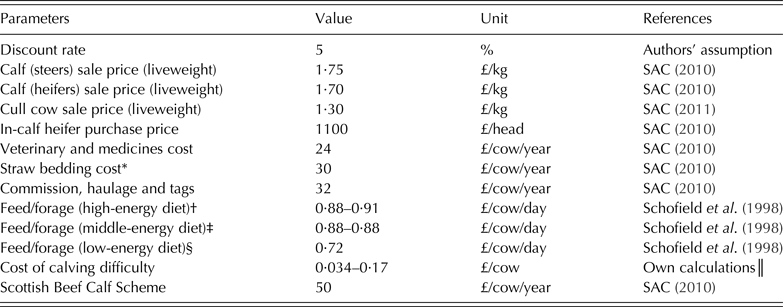
are coefficients for the kth parity and mth breed, respectively. The proportionality or equal slope assumption of the model was checked graphically. The model was parameterized in terms of ratios of lower to higher categories of CDS, i.e. normal to abnormal calving difficulty. Hence, a negative coefficient corresponds to less frequent abnormal calving, or more frequent normal calving. The fitted CLM was used to obtain the estimated probabilities of ordinal levels of CDS at each level of parity and BCS. Estimated probabilities of calving difficulties were used to calculate its annual cost per cow that is imposed on farmers (Table 1).
Financial and technical assumptions used in the dynamic programming model

* Straw bedding cost for in-house system.
† Assumed for BCS3 cows.
‡ Assumed for BCS2 cows.
§ Assumed for BCS1 cows.
║ Available from the corresponding author on request.
Calving periods
The length of the calving (mid-March to the end of May) was divided into four periods of 21 days, defined as ‘calving periods’. Based on the data, four calving periods (n
i
= 4) and one barren state were considered. To estimate the probability that a cow calves in a given calving period conditional on other explanatory variables, the generalized linear modelling framework described earlier was extended. Let π
i
be the probability that the cow was diagnosed as pregnant following AI, and
 ${\rm logit}(\pi _i) =\sum\nolimits_{k = 1}^{10} $
 ${\beta _kp_{ik}} + \sum\nolimits_{l = 1}^4 {\vartheta _ls_{il}} + \sum\nolimits_{m = 1}^3 {\omega _mb_{im}} $
where p
ik
was 1 if the parity of the ith observation was k and 0 otherwise, s
il
was 1 if the BCS of the ith observation was l and 0, otherwise, b
im
was 1 if the breed of the ith observation was m and 0 otherwise, and β
k
,
 $\vartheta _l$
and ω
m
were coefficients for the kth parity, l-th BCS and mth breed, respectively. It was also assumed that coefficients β
k
,
 $\vartheta _l$
and ω
m
were constant across all calving periods, and so the probability that a cow calved at each of the four calving periods was constant. It was assumed that all cows must be either in one of the calving periods or at barren stage in a given parity. To allow some barren cows to be retained in the data, it was also assumed that cows diagnosed as non-pregnant in a breeding season had the same chance of getting pregnant in the next breeding season as a non-barren cow. Although this is a considerable assumption given that the reasons for failure to breed may persist into the next breeding season, few such cases were observed in the present data set, and these data were penalized in the DP in other ways, i.e. through their contribution to involuntary culling, incurred variable costs and reduced stage returns as a result of their minimum reproduction performance. It is a common practice among some suckler beef farmers to keep infertile cows and mate them again during the next breeding season. Stott et al. (Reference Stott, Gunn and Barbudo2008) reported that the proportion of barren cows put to the bull on 66 Scottish suckler herds varied from 0 to 0·69. Hence, the probability that a cow calved at the n
i
th calving period was: π
i
(1 − π
i
)(n
i
−1). For N independently recorded observations, the likelihood function therefore was
 $L = \prod\nolimits_{i = 1}^N {\pi _i{(1 - \pi _i)}^{(n_i - 1)}} $
. The parameters of the model were estimated by maximizing the likelihood function using a simplex algorithm proposed by Nelder & Mead (Reference Nelder and Mead1965). The fitted model was used to obtain the probability of transition from the one calving period state (conditional on the parity and BCS) to all possible future calving period states.
Optimization model
A DP model was developed and used. Dynamic programming uses the repetitiveness of the decision to save computation time. It uses Bellman's Principle of Optimality (Bellman Reference Bellman1957): ‘an optimal policy has the property that, whatever the initial state and initial decision are, the remaining decisions must constitute an optimal policy with regard to the state resulting from the first decision’. This makes it possible to obtain the optimal policy by backward recursion from the optimal strategy in the final stage through to all possible states in the current stage, thus greatly reducing the computation required compared with a total enumeration of the problem. For further explanation and a simplified worked example see Stott et al. (Reference Stott, Jones, Humphry and Gunn2005). The present DP model is an extension of the models described by Stott (Reference Stott1994), Stott et al. (Reference Stott, Jones, Gunn, Chase-Topping, Humphry, Richardson and Logue2002) and Stott et al. (Reference Stott, Jones, Humphry and Gunn2005) that was adapted and parameterized to model the suckler cow replacement decision problem. A mathematical representation of the model is given in the Appendix. The objective of the DP was to maximize the expected gross margins (i.e. ENPV of returns expressed as an annuity) from a current suckler cow and future cows over an infinite time horizon by making appropriate replacement decisions.
This DP model drew on a closely monitored farm where recorded data, particularly on fertility in relation to parity, calving period and AI as well as on incidences of calving difficulty, were available to parameterize the model. Commercial practice (Barbudo et al. Reference Barbudo, Gunn and Stott2008) suggests that theoretical fertility performances suggested in the literature (e.g. Sinclair et al. Reference Sinclair, Molle, Revilla, Roche, Quintans, Marongiu, Sanz, Mackey and Diskin2002) are not entirely matched with actual farming practices, and therefore, an empirical approach was taken in the current work by using recorded data, rather than a theoretical one.
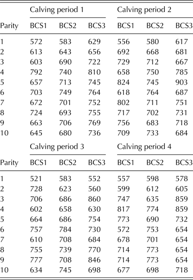
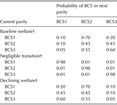
The possible decision options were either to ‘keep’ the current cow, or ‘replace’ her with an in-calf heifer at the start of each stage (annual production cycle). In either case involuntary replacement was still possible as a result of failure during the calving interval due to death, serious disease, injury etc. The probability of involuntary replacement was estimated from the GLM of the data described earlier and was used in the DP model as probability of failure for parity one to ten. The financial stage return thus included the expected (probability weighted) cost of involuntary replacement following failure. Cows were represented by 150 states in the DP including: ten states of cow parity, four states representing all possible 21-day calving periods in any parity plus one barren-cow status and three states for BCS. States of cow parity represented the maximum productive lifespan of individual cows, while five states of calving period, including barren status, influenced the probabilities of moving from current states into future calving states, henceforth called ‘transition probabilities’, were proxy for fertility (see Stott et al. Reference Stott, Veerkamp and Wassell1999). Three BCS states, consisting of low, middle and high, represented approximately the overall body condition of the cow during any stage. State-specific herd management input parameters including feeding regime, and hence cow-calf performance (Table 2) and feed costs, were included in the financial stage returns for each cattle state in the DP (see the next section). The transition probabilities for BCS that were used in the DP model (Table 3), represented the tendency for high, medium or low BCS to remain in that state or move to another state.
Arithmetic averages of suckler cow live weight (kg) based on parity, calving period* and body condition score (BCS) derived/estimated from the data and used in the dynamic programming (DP) †

* It was assumed barren cows have the same weight as cows calved in calving period 4.
† All these figures are based on historic data subject to the non-optimal culling policy operated on the herd. If DP was applied then these parameters would change, i.e. our results based on future culling are biased by historic parameter estimates. (This was discussed in Kennedy & Stott Reference Kennedy and Stott1993.)
Transition probability matrix* of body condition scores (BCS) used in the model

* The data set did not supply these data. Above assumptions were used to represent three scenarios with respect to animal welfare and the impact was examined in sensitivity analysis.
† Three animal welfare scenarios were examined with respect to transition probabilities from current BCSs to the next.
Stage return
To establish the stage returns, least-cost diet formulations were obtained using the ‘FeedByte’ software (Schofield et al. Reference Schofield, Calder, Fraser, Lewis, Oldham, Offer and Rooke1998) from the Scottish Rural College (SRUC) to obtain the gross margin of calf sales over feed supplementation and other variable costs for all possible 150 states. Barren cows incurred only maintenance costs, resulting in negative gross margins reflecting their non-productive status. Calf sale outcomes were calculated using an average of male and female calves' weight (data not presented) based on their market prices in 2010. This was done with a spreadsheet budget model in gross margin format using parameter estimates obtained either from the literature (Table 1) or from a survey of reproductive management in 66 spring calving commercial Scottish suckler herds reported by Barbudo et al. (Reference Barbudo, Gunn and Stott2008). The expected cost of involuntary replacement, i.e. net involuntary replacement cost weighted by the probability of involuntary replacement (P) was included in all stage returns. In addition, the net cost of voluntary replacement weighted by 1−P was included in stage returns when the decision was to replace. Net replacement cost was calculated for both voluntary and involuntary culling (represented by S and S′ in the Appendix) and replacement as the product of the live weight of the animals in different states (Table 2) and the cull cow price (£ per kg). If the replacement was involuntary, a loss of 3% in live weight was considered. This is due to premature cull value loss reported for Johne's disease (Bennett Reference Bennett2003) based on an assumption that the majority of these culls were due to diseases such as Johne's. The decision to keep or replace a cow is taken by the DP based on the probability adjusted stage return that is determined by both probabilities of survival or failure, as a result of diseases for example, and the marginal returns of the animals in various states, based on their weights and incurred variable costs. Keeping a cow for parity imposes extra costs, particularly for barren cows, and therefore the DP model optimized the culling and replacement decision.
The DP model was run using general purpose DP software (GPDP; Kennedy Reference Kennedy1986). An optimal culling strategy, ENPVs and infinite state probabilities were thereby generated. By changing key parameters in the DP and re-optimizing, the impact of alternative assumptions and management strategies, including over-wintered body condition, was explored. The DP runs included a baseline model run, three animal welfare scenarios and sensitivity analysis scenarios. Three animal welfare scenarios (Table 3) were examined with respect to transition probabilities from current BCS to the next. These included baseline welfare, negligible transition and declining welfare. Sensitivity of a model's outcome to the input variables, including calf sale price, feed price, heifer purchase price, cull cow price and Scottish beef calf scheme was tested by implementing a series of model runs using alternative input parameter values. The scenarios tested were 50 and 100% decrease and increase in the actual default values used for the baseline scenario.
Validation of the DP model was done by reviewing assumptions and input parameters, both from the data set and statistical models, as well as by comparing results or data from other sources and references to the outputs of the DP model. To do this, optimized (long-run state probabilities, which are fixed in this stationary DP model, see Stott et al. Reference Stott, Jones, Humphry and Gunn2005) proportions of animals in each of the four calving periods 1–4 and barren states, generated by the DP model, were compared with a benchmarking tool, the actual data used in the present paper, and observed commercial data. These were: (i) SRUC's target for herd fertility (Riddell et al. Reference Riddell, Caldow, Lowman, Pritchard and Morgan2013), (ii) SRUC's Easter Howgate actual data that were analysed and used in the DP model and (iii) a survey of Scottish commercial breeding suckler herds (Barbudo et al. Reference Barbudo, Gunn and Stott2008). The aim was to provide a basis for comparisons that helped to validate the DP model.
RESULTS
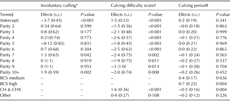
Estimated effects and standard errors (s.e.) of explanatory variables including parity, BCS, breed and others using the GLM and CLM for the three response variables including the incidence of involuntary culling, CDS and calving period are presented in Table 4. For the model on involuntary culling, the intercept value indicates the mean proportion of involuntary culling (on the logit scale) of cows at the reference level of Parity 1. Weak evidence (P = 0·067) was observed of an effect of parity on the mean proportion of involuntary culling of cows. Compared with parity 1, the mean proportions of involuntary culling cases did not differ significantly in parities 2–6, 8 and 9 (P ⩾ 0·170), but it increased significantly in parity 7 (P = 0·042) and parity 10 or more (P = 0·002). There was no evidence that BCS (P = 0·143) or breed (P = 0·660) influenced the mean proportion of involuntary culling in the studied suckler cow herd and therefore they were removed from the final analysis.
Estimated effects ( s.e. ) and associated P-values of explanatory variables from the fitted statistical models for three response variables

BCS, body condition score.
* The intercept value indicates the mean proportion of involuntary culling (on the logit scale) of cows at the reference level of Parity 1. The final model does not include BCS and Breed.
† The intercept value is the coefficient for the CDS score between 1 and 2 (1|2), which indicates the cumulative mean proportion (on the logit scale) of cows with CDS less than a given score at reference levels of other factors (Parity 1, Breed AAX). Estimates and s.e. of other intercepts are: 2|3 (2·02; 0·25) and 3|4 (3·28; 0·32). The final model does not include BCS.
‡ The intercept value indicates the mean proportion of successful conception (on the logit scale) of cows at reference levels of other factors (Parity 1, BCS Low, Breed AAX). The final model includes all factors, i.e. Parity, BCS and Breed.
§ Parity: Ten levels (1,…, 10); BCS: three levels (low, medium, high); Breed: three levels (AAX, Aberdeen Angus and its crosses; CH & CHX, Charolais and its crosses; Other, Limousin, Simmental and other crosses.
The CLM showed that breed (P < 0·001) and parity (P < 0·001) had a statistically significant effect on the mean proportion of CDS. However, there was no evidence that BCS had an effect on CDS (P = 0·408). Table 4 presents the estimated effects ( s.e.) of different explanatory variables on the CDS and associated P-values. The intercept value is the coefficient for the CDS score between 1 and 2 (1|2), which indicates the cumulative mean proportion (on the logit scale) of cows with CDS less than a given score at reference levels of other factors (Parity 1, Breed AAX). Compared with AAX (Aberdeen Angus and its crosses) and other (Limousin, Simmental and other crosses) crossbreds, there was strong evidence (P < 0·001) that cows of CH & CHX (Charolais and its crosses) were more prone to higher categories of CDS, i.e. abnormal calving difficulty. Results also showed that cows on parities 2 onwards (P < 0·010) were more likely to have lower CDS compared with cows on parity 1. This suggests that the probability of lower CDS increased with subsequent parities of cows.
Table 4 presents the estimated effects ( s.e.) of different explanatory variables on the calving period and associated P-values. The intercept value indicates the mean proportion of successful conception (on the logit scale) of cows at reference levels of other factors (Parity 1, BCS Low, Breed AAX). Results showed that BCS had a statistically significant effect (P = 0·009) on the mean proportion of successful conception following AI. Cows with low BCS had a significantly lower conception rate than cows with middle (P = 0·036) and high (P = 0·004) BCS. Weak evidence (P = 0·063) was found for a breed effect on the mean proportion of successful conception. The mean conception rate of cows of CHX breed was lower than cows of AAX breed (P = 0·004). The data did not suggest (P = 0·970) that the mean conception rate changed across parities.
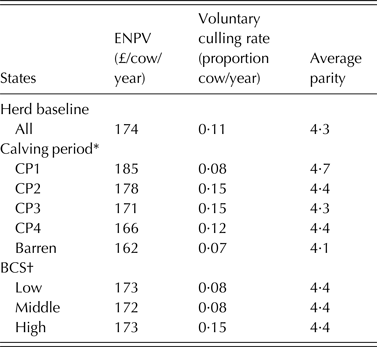
The results of the DP model runs showed that the ENPV, expressed as an annuity in the baseline welfare scenario (Table 3), was estimated to be £174 (±2·4 s.e.) per cow per year (Table 5). Cows calving in calving periods 1 and 2 were more profitable than the average profitability per cow at herd level. Late calving in periods 3 and 4 generated return below the average and barren cows had the lowest gross margin. Early calving favoured a ‘keep’ decision (cows calving in calving period 1 had a voluntary culling rate of 0·08 when the herd average was 0·11). Thus, very early calving cows were allowed to remain and live longer than the average age in the herd (4·7 and 4·3 parity, respectively). A possible reason is that early calving gives higher stage return (i.e. profit) due to heavier calves and a higher chance for early calving in later stages. Barren cows had the lowest voluntary culling rate (0·07), as optimized by the DP model, due to their low maintenance cost and their assumed potential to calve early in the next stage. Conversely, the model gave calving states 2, 3 and 4 (i.e. later calving periods) more ‘replace’ decisions, resulting in higher than the average herd-level voluntary culling rate (0·15, 0·15 and 0·12, respectively) in these states with less chance of early calving in subsequent stages. An explanation for slightly lower voluntary culling rate of cows in calving period 4 (0·12) than cows in calving periods 2 and 3 (0·15) is that the average weight of their calves over the ten parity in BCS1 and BCS2 states were higher (Table 2) and therefore had the potential of generating higher profit. Optimized results of the DP model also suggested that animals with a higher BCS were more prone to be voluntarily culled than animals with low and middle BCS. This is mainly due to the potential of high BCS animals to generate more profit because of their higher live weight than animals in middle and low BCS categories.
Expected financial performances (annuity of NPV in an infinite time horizon), voluntary culling rates and parity of cows in five states of calving period and three states of body condition score (BCS) under the baseline welfare scenario

NPV, net present value; ENPV, expected net present value.
* Four 21-day intervals and one barren state.
† Using 1–5 scale: low: <2·5; middle: 2·5–3·25; high: >3·25.
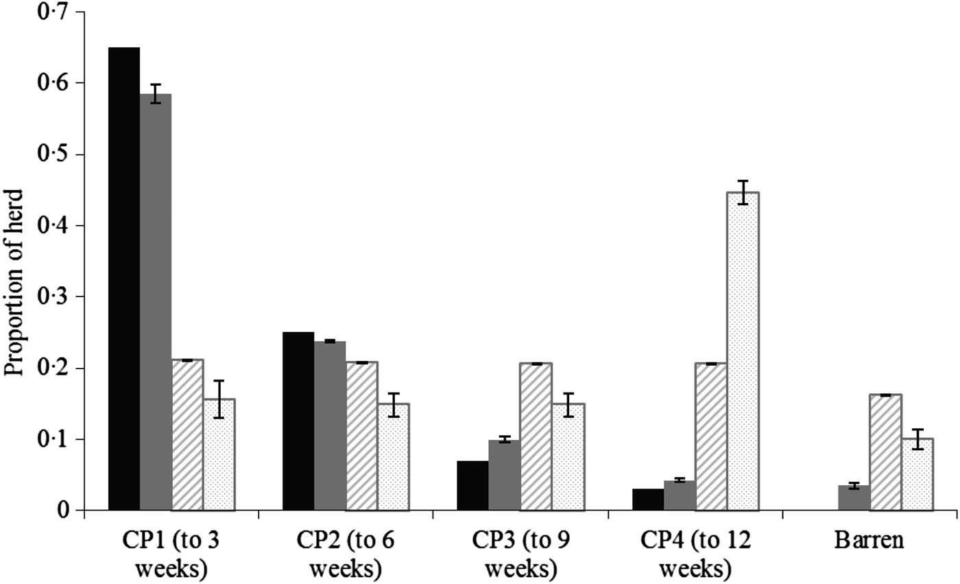
A comparison of the optimized proportions of animals in each of the four calving periods 1–4 and barren states with three alternative sources is presented in Fig. 1. The main emphasis on the Fertbench tool as a benchmark target is to have the majority of the animals (0·65) calving in the first period, 0·25 in the second, 0·07 in the third and 0·03 in the fourth period without keeping cows in a barren state. The comparison showed that the Easter Howgate actual data and the Fertbench target values followed a very similar pattern in terms of proportions of animals in each calving period. The DP's long-term optimized results, however, have more similarity to the calving patterns of commercial beef sucker farms. One reason for the differences between the background data and optimized results could be that the advantages of early calving (suggested by the Easter Howgate actual data and achieved by using AI) are not sufficient to justify the costs of expected heavier culling rates. The long-run results of the DP had equal proportions of animals (0·21) in calving periods 1–4 and 0·16 in the barren state. The DP's long-run state probabilities are the outcome of the optimal culling regime given the fixed assumptions used in the DP model and the management of the SRUC herd. This may make it uneconomic to improve because the advantages of early calving are not sufficient to justify the costs of heavier culling rates. The commercial herd survey had 0·15 of the herd in calving periods 1–3, but a large proportion (0·45) in the calving period 4, and 0·1 in the barren state.
Calving pattern of Scotland's Rural College's Fertbench targets (black solid bars), compared with the current analysed data set of Easter Howgate herd (solid grey bars), the optimized results of the dynamic programming model baseline welfare scenario (dashed bars) and the results of a survey of commercial Scottish breeding suckler herds performed in 2005 (Barbudo Reference Barbudo2005) (dotted bars). Error bars represent s.e. of means.

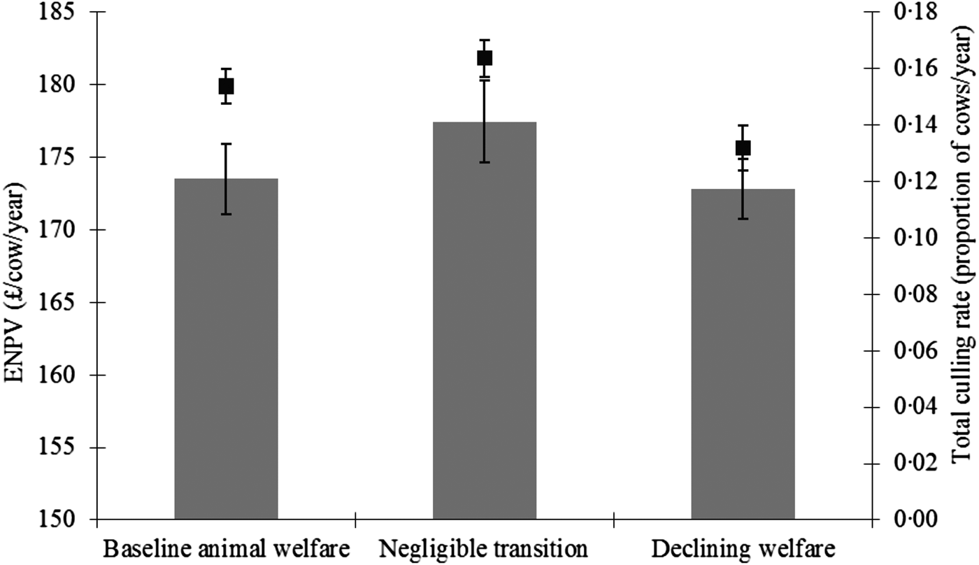
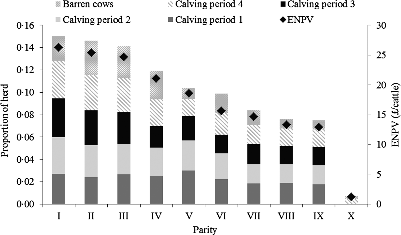
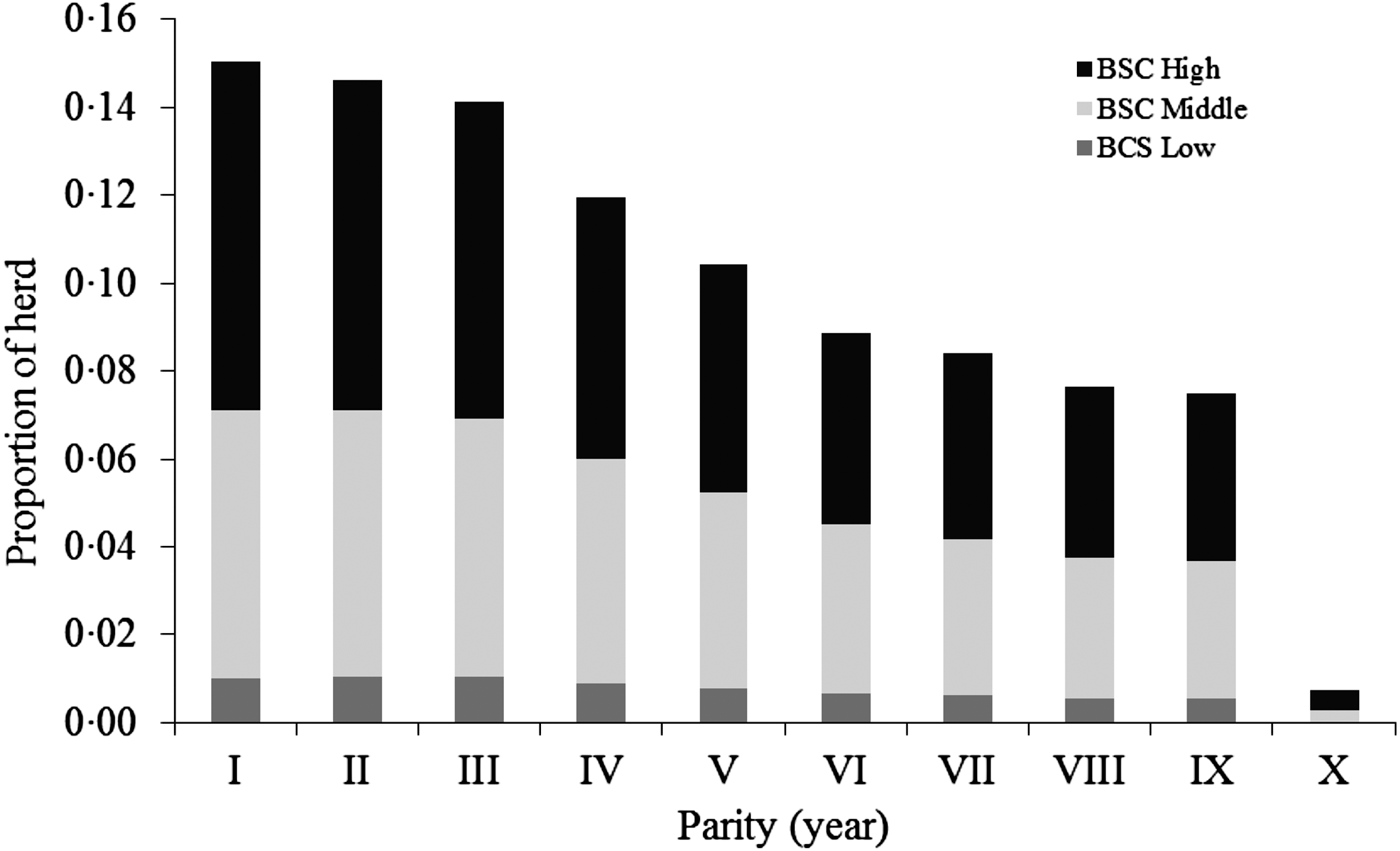
Three animal welfare scenarios (Table 3) were examined with respect to transition probabilities from current BCS to the next. Results (Fig. 2) suggested that the scenario of negligible or minimum transition between BCS states generated the highest financial return (£177/cow/year) compared with the baseline and declining welfare scenarios (£174 and £172, respectively). The minimum transition welfare scenario incurred the highest total culling rate at 0·16 compared with 0·15 and 0·13 for the baseline and the declining welfare scenarios, respectively. The optimized results under the baseline welfare scenario showed that approximately 0·56 of the animals were in parity 1–4 (Fig. 3), while >0·92 animals had middle or higher BCS in each parity (Fig. 4).
Expected net present value £/cow/year ± s.e. (bars) and estimated total culling rates ±s.e. (■) under three scenarios using different transition probabilities for body condition scores presented in Table 3. Error bars represent s.e. of means.

Optimum proportion of herd based on five calving period categories and parity and expected net present value per parity predicted by the dynamic programming model under baseline welfare scenario as given in Table 3.

Optimum proportion of herd (i.e. final distribution in long-term after all culling and replacement decisions have been taken) based on body condition score category and parity predicted by the dynamic programming model under baseline welfare scenario as given in Table 3.

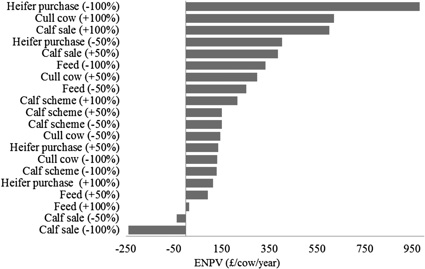
The results of the sensitivity analysis showed that the financial returns were highly sensitive to a decrease of heifer purchase/rearing price, increase in cull cow price and calf sale price (Fig. 5). Results were also sensitive to decrease in feed costs and increase in subsidy.
Sensitivity of the expected net present value to input parameters. The scenarios tested were 50 and 100% decrease and increase in the actual default values used for the baseline scenario.

DISCUSSION
The present paper analysed a 5-year production database of a closely monitored breeding beef suckler cattle herd, estimated probabilities of involuntary culling and calving difficulty and transition probabilities between different state variables, and subsequently parameterized a DP model to analyse potential interactions and trade-offs between fertility, animal welfare and profitability of suckler cattle.
The analysis showed the probability of successful conception in each of the four 21-day periods after post-partum anoestrus (followed by successful calving) was not influenced by parity. This is contrary to the common expectation that the probability of conception declines as a cow ages at subsequent parities. In agreement with the current results, Drennan & Berry (Reference Drennan and Berry2006) also found that cow parity did not affect the fertility rates of breeding suckler cows. Cows on parities 2 onwards were more likely to have lower CDS compared with cows on parity 1. The likelihood of increased calving difficulty at the first parity has practical and welfare implications, as higher incidence of calving difficulties in the first parity will result in increased culling and replacement rate. On the other hand, later parities increased the frequency of involuntary culling marginally, particularly for the cows of parities 7 and 10 or more, thus incurring extra losses. Additionally, a biased effect of parity on involuntary culling probabilities could also result from the statistical modelling of the data, which were already constrained by culling due to infertility or other health problems.
It was observed that cows having low BCS had lower conception rates compared with cows having middle and high BCS. In contrast, no evidence was found that BCS had an effect on the probability of involuntary culling or CDS. This suggests that associating BCS with welfare related problems of cows such as lameness and other natural threats were not mirrored in the herd used for the current work. This may be a reflection of reduced variability in BCS in this closely monitored herd compared with commercial practice.
Optimized results of the DP model indicate that very early calving animals (conception within 21 days after the post-partum anoestrus period) contribute to maximizing the financial profitability of beef suckler herd as well as reducing the voluntary culling rate. Results also showed that reducing the voluntary culling rate is attributed to fewer animals in their first parity and thus the lower calving difficulty in subsequent parities. This is a win–win scenario for profit and welfare. In order to obtain the best result, an increased calving rate in the first calving period could be achieved by aiming to have a larger proportion of cows in parity 2–4 and middle BCS at weaning.
The expected trade-off between animal welfare, fertility and profitability was not apparent in the current results. Animals with low BCS suffered from lower nutrient intake (lower welfare), but were also less profitable than animals with higher BCS. Achieving such improvements in BCS depends on a high-energy feed regime in the winter time, which adds some extra costs, but these were outweighed by improved technical performances such as having a higher calf weight at birth as well as higher calf growth rate, and eventually, a higher generated revenue at sale. Obviously, the current results are dependent upon the assumptions made and the herd-specific relationships incorporated in the model. There may well be circumstances in practice whereby improving welfare reduces the profit and therefore a trade-off occurs. However, such trade-offs (i.e. opposite effects of welfare and profit; see McInerney (Reference McInerney2004)) are not inevitable, and there are probably many opportunities such as this to obtain a win–win for profit and for welfare in current farming practice. Lawrence & Stott (Reference Lawrence and Stott2009) provided the data and analytical tools to understand the key relationships involved and use them to adjust management towards more sustainable, productive and efficient outcomes.
It was assumed that a high BCS state implied better animal welfare status. The presented optimized results of the DP model, however, suggest that animals in such herds are more prone to be culled (voluntarily here, but could be culled on an involuntary basis too) and replaced by heifers, and thus their longevity is shorter than the low BCS states. In so far as longevity is a mark of good welfare, there is a potential conflict here, i.e. overall welfare may not be adequately captured by one index alone. This issue has been dealt with elsewhere, e.g. by Vosough Ahmadi et al. (Reference Vosough Ahmadi, Stott, Baxter, Lawrence and Edwards2011) and Stott et al. (Reference Stott, Vosough Ahmadi, Dwyer, Kupiec, Morgan-Davies, Milne, Ringrose, Goddard, Phillips and Waterhouse2012). However, as with any model, the current one was a simplification of the true situation, for example, interactions among all the modelled variables that could exist in practice were not modelled.
As well as difficulties with welfare assessment, the current results can be used in highlighting possible conflicts and also synergies between policy on animal welfare and policy on other important issues such as the environment and sustainable intensification. The sustainable intensification concept incorporates the ambition to increase or maintain the current level of agricultural yields while reducing negative ecological and environmental impacts (Vosough Ahmadi et al. Reference Vosough Ahmadi, Moran, Barnes and Baret2015b ). Presented statistical models linked to a DP model showed that better financial and economic performances could be achieved with less feeding and lower BCS animals without compromising animal welfare as defined in the present paper. This was a result of having access to data from a well-managed farm and the described analyses and interpretations. In future, recording, collecting and analysing detailed bio-physical data will be essential part of farm management of commercial breeding suckler cattle farms that will be a key to sustainable intensification. Similarly the AI practice that was used in the studied farm, which is not currently commonly used in commercial farms, is made more feasible for suckler herds with new technologies. By integrating AI in reproduction management of breeding suckler cattle farms, it will be possible to get higher genetic gain, which will add to the merits of sustainable intensification.
Results presented in the present paper suggest that providing high-energy diet that leads to heavier cows with high BCS required more in-calf heifer replacements as a result of heavier culling rate. This will lead to a higher number of animals on the farm, compared to providing a low nutritional level, as farms under this management regime need to raise higher numbers of replacement heifers or buy them from the market. Because cattle have been identified as a threat to the climate, forests and wildlife (Gill et al. Reference Gill, Smith and Wilkinson2010; Foresight 2011), increasing the population of suckler cows as a result of a different feeding regime as well as culling/replacement strategies is detrimental to the environment. Herds with high BCS cows require more ‘bought-in’ roughage and concentrates during the winter time, and higher quantities of fertilizers and perhaps pesticides to grow grazing pastures in summer time. These all adversely affect the environment (e.g. air and water pollution), and therefore, the trade-offs between these environmental concerns and financial performance of the out-wintering suckler cows and their welfare concerns need to be studied further using an integrated framework.
CONCLUSIONS
The expected trade-off between animal welfare, fertility and profitability was not apparent in the current results. Animals with low BCS suffered from lower nutrient intake (lower welfare), but were also less profitable than animals with higher BCS. Achieving such improvements in BCS depends on a high-energy feed regime in the winter time, which adds some extra costs, but these were outweighed by improved performance such as having a higher calf weight at birth as well as higher calf growth rate, and eventually, a higher generated revenue at sale. There may well be circumstances in practice where a trade-off occurs. However, such trade-offs are not inevitable, and there are probably many opportunities such as this to obtain a win–win for profit and for welfare in current farming practice provided the data and analytical tools are available, as provided in the current work, to understand the key relationships involved and use them to adjust management towards more sustainable, productive and efficient outcomes. The main practical conclusion regarding herd management is that increasing the number of very early calving cows (those who conceived in the first 21 days after AI) by optimizing reproduction management improves both financial and animal welfare scores of suckler cattle farms. It can be concluded that good reproduction management could deliver a win-win situation with regards to profit, animal welfare and environment.
The authors thank the Scottish Government for funding this research. We are grateful to Dr John Kennedy for his scientific advice. We also thank Dr Sarah Brocklehurst for her critical comments on the manuscript. This research was undertaken within the Scottish Government Rural Affairs and the Environment Portfolio Strategic Research Programme 2011–2016, Theme 4: ‘Economic Adaptation’ and Theme 6: ‘Health and Welfare’. The first author currently works at the IPTS, JRC-European Commission but the views expressed in this paper are the sole responsibility of the authors and do not reflect those of the European Commission. The paper does not reflect the views of the institutions of affiliation of the authors either.
APPENDIX
The mathematical formulation of the DP model
 $$V_i\{ L_i,\;C_i,\;B_i\} = {\rm Max}\;[K\{ L_i,\;C_i,\;B_i\}, \;R\{ L_i,\;C_i,\;B_i\}, \;S\{ L_i,\;C_i,\;B_i\} ] \quad (i = {\rm 1}, \ldots, \;n)$$
where
For the decision to keep the cow for one or more lactations:
 $$\eqalign{K\{ L_i,\;C_i,\;B_i\} & = A\;\{ L_i,\;C_i,\;B_i\} \cr & + \alpha {\left\langle {\matrix{P\{ L_i\}. \left[ {\sum\limits_{L_{i + 1}}^{10} {\sum\limits_{C_{i + 1}}^5 {\sum\limits_{B_{i + 1}}^3 {P_c {\cdot} P_b\left\langle {B_{i + 1} \vert B_i} \right\rangle {\cdot} V_{i + 1}\{ L_i + 1,C_{i + 1},B_{i + 1}\}}}}} \right] \hfill \cr + (1 - P\{L_i\} ) {\cdot} \left[ {\left( {\sum\limits_{L_{i + 1}}^{10} {\sum\limits_{C_{i + 1}}^5 {\sum\limits_{B_{i + 1}}^3 {P_c \,{\cdot}\, P_b\left\langle {B_{i + 1} \vert B_i} \right\rangle} \,{\cdot}\, V_{i + 1}\{ 1,C_{i + 1,}B_{i + 1}\}}}}\right) - h + {S}^{\prime}\{ L_i,C_i,B_i\}} \right] \hfill}} \right\rangle}}$$
and for the decision to replace the cow:
 $$\eqalign{R\{ L_i,\;C_i,\;B_i\} &= A\{ L_i,\;C_i,\;B_i\} \cr & + \alpha \left\langle \matrix{\left[ {\sum\limits_{L_{i + 1}}^{10} {\sum\limits_{C_{i + 1}}^5 {\sum\limits_{B_{i + 1}}^3 {P_c \,{\cdot}\, P_b\left\langle {B_{i + 1} \vert B_i} \right\rangle \,{\cdot}\, V_{i + 1}\{ L_1,C_{i + 1},B_{i + 1}\}}}}} \right] - h + P\{ L_i\} S\{ L_i,C_i,B_i\} \hfill \cr + (1 - P\{ L_i\} ) {\cdot} {S}^{\prime}\{ L_i,C_i,B_i\} \hfill} \right\rangle}$$
where
 $$\eqalign{A\{ L_i,\;C_i,\;B_i\} & = cw\{ L_i,\;C_i,\;B_i\} p + a \cr & \quad- f\;\{ L_i,\;C_i,\;B_i\} - z}$$
Key to symbols in the above equations: