1 Introduction
In offshore operations, gaps between parallel ship-shaped floating bodies will occur in side-by-side offloading (e.g. from a floating liquefied natural gas (FLNG) facility to an LNG carrier) or in floatover installation where parallel barges support topside modules during installation of the topsides onto the supporting space frame for large offshore structures. These operations are of limited duration and hence will not take place in extreme seas, but even in moderate sea states incident surface waves may excite resonant motions of fluid in the gap.
Gap resonance problems share some features with moonpool resonances, for which Molin (Reference Molin2001b ) derived an analytical formula to estimate the natural frequencies and associated modal shapes of the resonant modes based on linear potential flow theory. Modes with profiles both along and across the moonpool were found. To approximately predict the natural frequencies of the gap resonant modes, Molin (Reference Molin2001b ) and Molin et al. (Reference Molin, Remy, Kimmoun and Stassen2002) extended the approach for the moonpool problem by modifying the boundary conditions at the ends. A comprehensive study of the frequencies, modal shapes and response amplitudes for the free surface in the gap between two fixed vessels was made by Sun, Eatock Taylor & Taylor (Reference Sun, Eatock Taylor and Taylor2010) using potential flow diffraction theory at first and second order.
Several investigations into the behaviour of 2D geometries consisting of rectangular boxes separated by a gap have been made. This represents a 2D approximation of both moonpool and gap resonance problems, although it neglects any structure in the fluid motion along the gap. Several 2D investigations have shown that linear potential theory overpredicts experimentally determined peak resonant response amplitudes for sinusoidal excitation (Faltinsen, Rognebakke & Timokha Reference Faltinsen, Rognebakke and Timokha2007; Lu et al. Reference Lu, Teng, Sun and Chen2011). In 3D, the same effect has been reported for tests on side-by-side fixed vessels (Pauw, Huijsmans & Voogt Reference Pauw, Huijsmans and Voogt2007; Molin et al. Reference Molin, Remy, Camhi and Ledoux2009), although the overprediction is smaller.
Many methods to improve the level of agreement between potential flow calculations and the results of physical experiments have been proposed, including rigid (Huijsmans, Pinkster & De Wilde Reference Huijsmans, Pinkster and De Wilde2001) or flexible lids at each (generalised) mode (Newman Reference Newman and Kashiwagi2001) and a dissipative damping term in the free-surface condition (Chen Reference Chen2005). The selection of the additional damping coefficient is generally empirical, being based on a fit to model test data, emphasising the importance of model tests.
The possible sources of this discrepancy between linear potential theory and model tests are generally held to be viscous effects associated with flow separation and nonlinear free-surface boundary conditions. Much work suggests that flow separation is the main source of the discrepancy (Kristiansen & Faltinsen Reference Kristiansen and Faltinsen2008; Molin et al. Reference Molin, Remy, Camhi and Ledoux2009; Kristiansen & Faltinsen Reference Kristiansen and Faltinsen2012). In addition, Feng & Bai (Reference Feng and Bai2015) carried out fully nonlinear numerical simulations, and reported that nonlinearity may slightly increase the resonant frequency, though with limited effect on the amplitude. It seems that the accuracy of potential flow theory is dependent on the bilge shapes, i.e. it gives some overprediction for the round bilge case, where flow separation is less important, and greatly overestimates the resonant response amplitude for the square bilge case, where separation is inevitable. Without performing dedicated model tests, Faltinsen & Timokha (Reference Faltinsen and Timokha2015) estimated the damping coefficient for sharp cornered boxes by combining the approximation of Molin (Reference Molin2001b ) and the pressure drop coefficient formula for a slatted screen. Their estimation of the additional damping coefficient is, however, based on the behaviour of slatted screens, so still requires experimental calibration.
A comprehensive experimental investigation of gap response between a ship-shaped vessel and a large bottom-mounted rectangular box was carried out by Perić & Swan (Reference Perić and Swan2015). Tests were conducted with a fixed and floating ship, and for regular, irregular and focused incident waves. Several different mode shapes were identified experimentally, as well as contributions from higher harmonics.
While many research efforts into the gap resonant response have been undertaken, the majority have concentrated on analysis of the maximum gap resonant amplitude at steady state in regular waves. However, real ocean waves are not regular in general, and reaching steady state is not straightforward in tank experiments, due to the long time necessary to build up to maximum amplitude, by which time reflected waves may affect the experiments. There is interest in the behaviour of the fluid in the gap in transient wave groups, as considered by Eatock Taylor, Sun & Taylor (Reference Eatock Taylor, Sun and Taylor2008), who numerically studied the gap resonant response under focused wave groups, producing time series of the response using linear theory. Experimentally, wave groups have been used to test gap resonances by Clauss, Dudek & Testa (Reference Clauss, Dudek and Testa2013) and Perić & Swan (Reference Perić and Swan2015), although in these cases the emphasis was on deriving regular wave response coefficients from the results rather than on the gap behaviour. To the best of the authors’ knowledge, there are no experimental studies on the transient gap resonance problem that present time histories similar to those produced numerically by Eatock Taylor et al. (Reference Eatock Taylor, Sun and Taylor2008).
In light of the above, we carried out an extensive set of experiments to investigate the gap resonant response under transient focused wave groups, where higher harmonics have been extracted successfully. The set-up of the experiments is similar to Molin et al. (Reference Molin, Remy, Camhi and Ledoux2009) but our emphasis is different. Rather than seeking to derive response amplitude operators for the steady-state response of the gap, we are interested in the time-dependent response and nonlinear gap resonance phenomena, including the possibility of frequency doubling driving gap resonance. This study is organised as follows. Following this introduction, the experimental set-up in a wave basin is described in § 2. The theoretical background is presented in § 3, including the NewWave-type focused wave group generation and the four-phase combination methodology which is used for the isolation of the harmonics from complicated wave–wave and wave–structure interactions. Results are given in § 4 for different cases. First, we discuss the transient characteristics of the gap resonant response under excitation by a wave group with components around the resonant frequencies (§ 4.1). Then, we change the heading (§ 4.2), bandwidth (§ 4.3) and linear amplitude (§ 4.5) of the incident waves and finally the bilge shape of the boxes (§ 4.4). Inspired by interesting observations in § 4.5, we then investigate the transient gap resonant responses excited by a wave group with components of around half the frequencies of the gap resonant responses (§ 4.6) and the resulting higher harmonics and nonlinearities (§ 4.7). The decay rates of each gap resonance mode are investigated in § 4.8. Finally, § 5 presents some conclusions.
2 Experimental set-up
The experiments were carried out in the Deepwater Wave Basin at Shanghai Jiao Tong University. This wave basin is 50 m long, 40 m wide, and the water depth can be adjusted from 0 to 10 m using an artificial bottom; here, the depth was set to 10 m. Flap-hinged wavemakers are fixed along two neighbouring sides of the basin and wave absorbing beaches are installed on the opposite sides to minimise reflected wave energy from the boundaries of the basin.
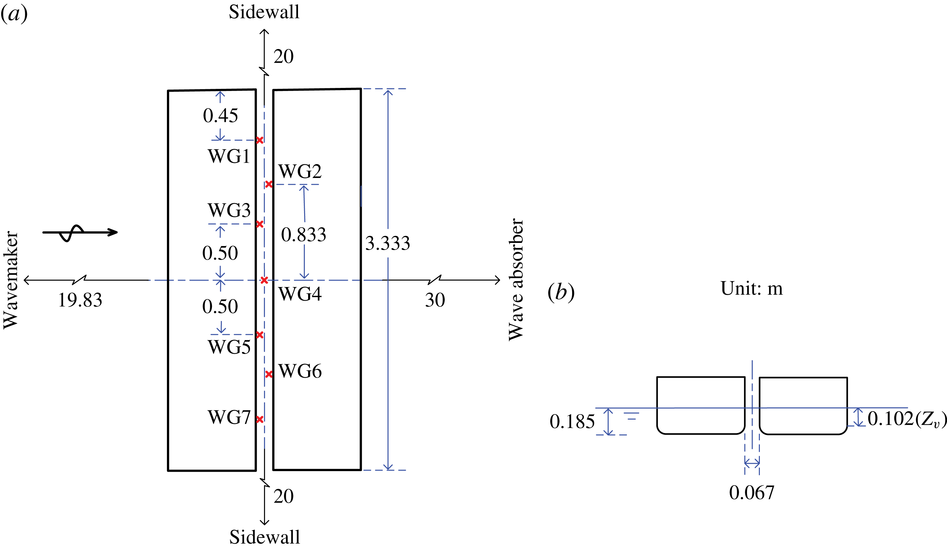
As shown in figure 1, two identical rectangular boxes were used in the experiments. The boxes are prismatic and are 3.333 m long. In cross-section they are 0.767 m wide with round corners (as default) at both bilges, each with a radius of 0.083 m running along the length. The two boxes are 0.425 m high and immersed such that the undisturbed draught is 0.185 m, leading to a 0.102 m high immersed vertical surface (height marked
 $z_{v}$
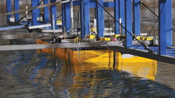
in figure 1). The two boxes were rigidly mounted on a gantry in the central area of the wave basin in a side-by-side configuration, forming a narrow gap of 0.067 m. The gantry is very robust, so provided enough stiffness to prevent vibration of the box models at wave frequencies. The midpoint of the gap was 19.83 m away from the wave paddles and 20 m from the sidewalls of the wave basin. A snapshot of the box hulls is shown in figure 2, where both the gantry and the small gap between the boxes are visible.
Sketch of the two identical side-by-side fixed box hulls in the wave basin in (a) plan view and (b) end elevation. The wave gauge (WG) positions within the gap are identified. Not to scale.

A snapshot of the two box hulls (yellow) rigidly connected to the gantry (blue).

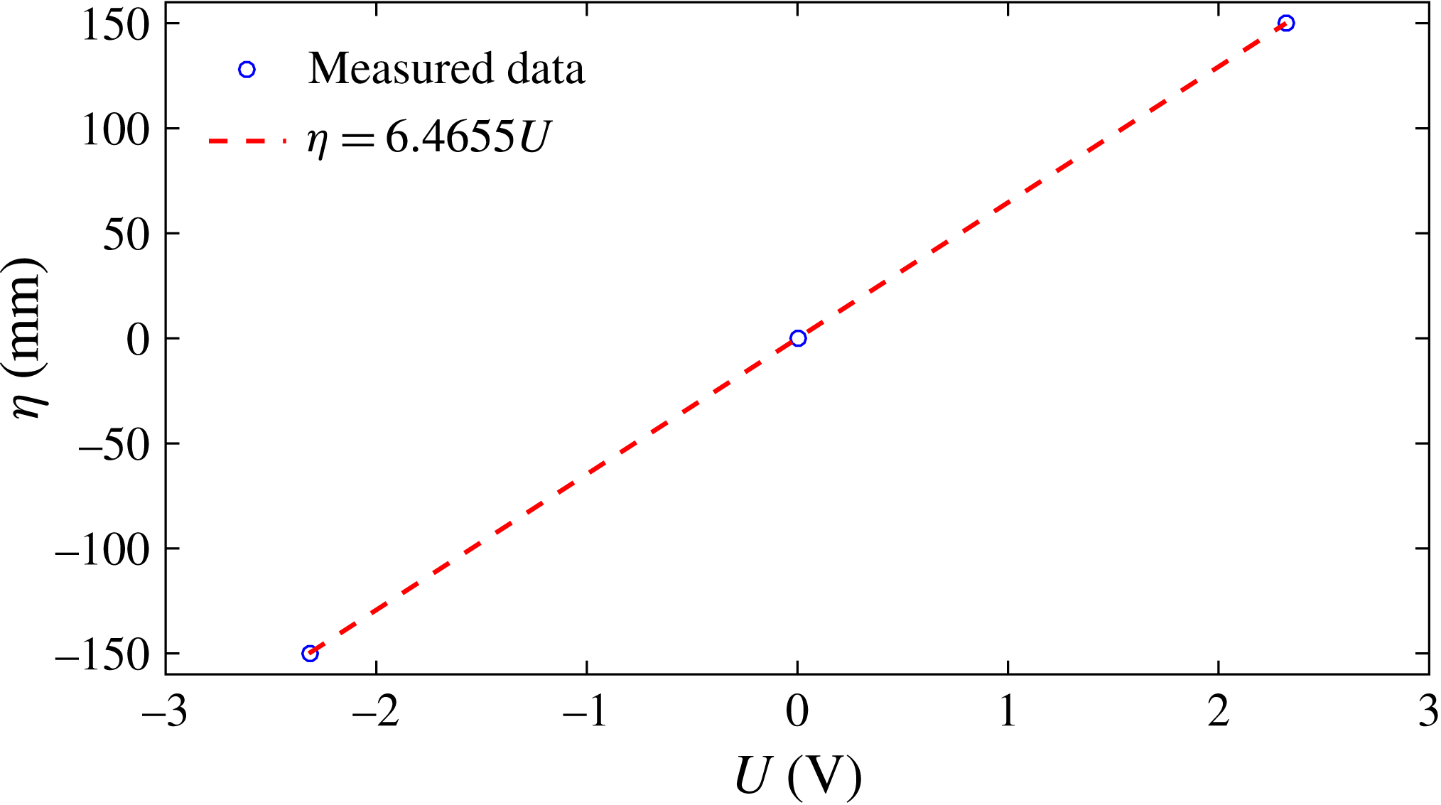
We use standard resistance-type wire probes to record the water surface elevations. As shown in figure 1, wave gauges (WGs) 1 and 7 are 0.450 m from the ends of the gap (1.216 m from the centre), WGs 2 and 6 are 0.833 m from the centre of the gap, WGs 3 and 5 are 0.500 m from the centre of the gap and WG4 is central. The wire probes have a measurement error of less than 1 mm. To check linearity, the wire probes are calibrated prior to the measurements, and a representative calibration result is shown in appendix A. The transient wave groups are generated both with and without the vessel models in place, and the wave paddle and surface elevation gauge signals are recorded synchronously.
The experimental models represent 1 : 60 scaled versions of generalised but realistic vessels, meaning that the gap is very narrow, at approximately 4 m at full scale. We emphasise that testing such a narrow gap requires a large-scale experiment, and, therefore, particularly in beam seas, a large basin. There have been few tests with such parameters.
3 NewWave theory and harmonic extraction method
NewWave focused wave groups (Jonathan & Taylor Reference Jonathan and Taylor1997) are used as the input waves. The higher harmonics are then extracted from the measured gap resonant responses.
3.1 NewWave focused wave group
In a random sea with given power spectral density
 $S(f)$
, the average shape of the largest wave is a scaled autocorrelation function (Lindgren Reference Lindgren1970; Boccotti Reference Boccotti1983; Tromans, Anaturk & Hagemeijer Reference Tromans, Anaturk and Hagemeijer1991), assuming that the underlying sea-state surface elevation corresponds to a linear random Gaussian process. A large wave crest occurs at the focus position and time (
 $x_{0}$
,
 $t_{0}$
) with phase
 $\unicode[STIX]{x1D713}=0$
. The shape of a unidirectional NewWave group is given by
 $$\begin{eqnarray}\unicode[STIX]{x1D702}_{N}(x,t)=\frac{\unicode[STIX]{x1D6FC}}{\unicode[STIX]{x1D70E}^{2}}\mathop{\sum }_{n=1}^{N}S(f_{n})\unicode[STIX]{x0394}f\,\text{Re}[\text{e}^{-\text{i}k_{n}(x-x_{0})+\text{i}2\unicode[STIX]{x03C0}f_{n}(t-t_{0})+\unicode[STIX]{x1D713}}],\end{eqnarray}$$
where
 $\unicode[STIX]{x1D702}_{N}(x,t)$
indicates the free-surface profile of the NewWave-type focused wave group,
 $\unicode[STIX]{x1D6FC}$
corresponds to the expected maximum free-surface elevation in a given sea state,
 $k_{n}$
and
 $f_{n}$
are the wavenumber and frequency of the spectral component, and the variance
 $\unicode[STIX]{x1D70E}^{2}=\sum _{n=1}^{N}S(f_{n})\unicode[STIX]{x0394}f$
.
In this study, we concentrate on the gap resonant response under NewWave-type wave group excitation. While gap resonance is likely to be relevant only in moderate sea states in practice, the largest events in these sea states will be well described by NewWave. In fact, NewWave should be a better model for the largest waves in a moderate sea state than in limiting steepness cases because nonlinear effects are likely to be much weaker (at least close to the focus). The focus position of the NewWave group was set at
 $x_{0}=19.83$
m from the equilibrium position of the wave paddles, i.e. the centre of the gap.
In the experiments, we used two shapes for the model corners, i.e. round corners and square corners, two headings for the models, i.e. waves approaching the gap laterally (broadside to the vessel models, so beam seas) and waves approaching the gap longitudinally (head seas), two (nominal) maximum amplitudes for the NewWave groups, i.e.
 $\unicode[STIX]{x1D6FC}=50$
mm and
 $\unicode[STIX]{x1D6FC}=100$
mm, and two spectral peak frequencies for generating the NewWave groups, i.e. peak frequencies identical to the first mode of the gap resonance (
 $f_{P}=f_{m=1}$
) and half of this value (
 $f_{P}=0.5f_{m=1}$
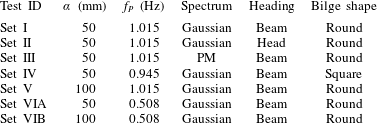
). The seven combinations of the above parameters implemented in the tests are summarised in table 1, with four different phase realisations contained in each set. Combinations of the different phase realisations will be used for the extraction of the harmonic components, which will be addressed in detail in the following section.
Incident waves and the corresponding experimental set-up. Here,
 $\unicode[STIX]{x1D6FC}$
stands for the (nominal) maximum surface elevation,
 $f_{P}$
is the peak frequency of the spectrum used for the generation of the transient wave group and PM indicates Pierson–Moskowitz.

For the cases in table 1, the Gaussian spectrum used for the generation of the NewWave group is given by the following equation:
 $$\begin{eqnarray}S(f)=\frac{H_{s}^{2}}{16}\frac{1}{\sqrt{2\unicode[STIX]{x03C0}\unicode[STIX]{x1D6FF}^{2}}}\exp \left(-\frac{(f-f_{P})^{2}}{2\unicode[STIX]{x1D6FF}^{2}}\right),\end{eqnarray}$$
where
 $H_{s}$
refers to the significant wave height,
 $f_{P}$
is the peak frequency of the spectrum and
 $\unicode[STIX]{x1D6FF}=0.0775$
Hz is the (laboratory scale) shape parameter of the Gaussian spectrum used in this study.
3.2 Extracting higher harmonics
For each ‘set’ in table 1, four different NewWave groups were generated using the same paddle signal, but with each component shifted by a relative phase
 $\unicode[STIX]{x1D713}$
of
 $0^{\circ }$
,
 $90^{\circ }$
,
 $180^{\circ }$
or
 $270^{\circ }$
respectively. This corresponds to a crest focus, a trough focus and up- and down-crossings, all with the same linear envelope. The linear component and nonlinear harmonics of the incident wave and response are extracted by linear combination of the four-phase time histories. This process assumes that the weakly nonlinear waves and wave–structure interaction may be described by a Stokes-type expansion of the surface elevation, written here up to the fourth order in linear component amplitude
 $A$
:
 $$\begin{eqnarray}\displaystyle \unicode[STIX]{x1D702}(\unicode[STIX]{x1D703}) & = & \displaystyle A\unicode[STIX]{x1D702}_{11}\cos (\unicode[STIX]{x1D703})+A^{2}(\unicode[STIX]{x1D702}_{20}+\unicode[STIX]{x1D702}_{22}\cos 2\unicode[STIX]{x1D703})+A^{3}(\unicode[STIX]{x1D702}_{31}\cos \unicode[STIX]{x1D703}+\unicode[STIX]{x1D702}_{33}\cos 3\unicode[STIX]{x1D703})\nonumber\\ \displaystyle & & \displaystyle +\,A^{4}(\unicode[STIX]{x1D702}_{40}+\unicode[STIX]{x1D702}_{42}\cos 2\unicode[STIX]{x1D703}+\unicode[STIX]{x1D702}_{44}\cos 4\unicode[STIX]{x1D703})+O(A^{5}),\end{eqnarray}$$
where
 $\unicode[STIX]{x1D703}$
is the phase function of the incoming wave and the
 $\unicode[STIX]{x1D702}_{ij}$
are the coefficients in the expansion.
It is straightforward to separate the higher harmonics for a regular wave, but it is slightly more complicated for wave groups, where the simple Stokes-type terms are replaced by summations of linear terms. Taking an irregular sea as an example, the Stokes-type expansion of the surface elevations up to second order in
 $kA$
can be given as (Fitzgerald et al.
Reference Fitzgerald, Taylor, Eatock Taylor, Grice and Zang2014)
 $$\begin{eqnarray}\displaystyle & \displaystyle \unicode[STIX]{x1D702}=\mathop{\sum }_{n=1}^{N}A_{n}\cos (\unicode[STIX]{x1D703}_{n})+\mathop{\sum }_{n=1}^{N}\mathop{\sum }_{m=1}^{N}[A_{n}A_{m}B_{nm}^{+}\cos (\unicode[STIX]{x1D703}_{n}+\unicode[STIX]{x1D703}_{m})+A_{n}A_{m}B_{nm}^{-}\cos (\unicode[STIX]{x1D703}_{n}-\unicode[STIX]{x1D703}_{m})],\quad & \displaystyle\end{eqnarray}$$
where
 $A_{n}$
refers to the amplitude of the free-wave component and
 $\unicode[STIX]{x1D703}_{n}=k_{n}x-\unicode[STIX]{x1D714}_{n}t$
its phase, where the angular frequency
 $\unicode[STIX]{x1D714}=2\unicode[STIX]{x03C0}f$
. Here,
 $B_{nm}^{+}$
and
 $B_{nm}^{-}$
define the contribution of the wave–wave interactions.
Assuming a narrowbanded power spectrum, the Stokes-type expansion can be generalised to a focused wave group. The phases for each free-wave component are chosen, so that the crests coincide at focus (
 $x_{0}$
,
 $t_{0}$
). Around the focus point, the signal envelope can be regarded as a slowly varying function of time, i.e.
 $A(t)$
. Therefore, the free-surface elevations up to second order at the focus position around the focus time can be given as follows:
 $$\begin{eqnarray}\displaystyle \unicode[STIX]{x1D702}=A(t)\cos (\unicode[STIX]{x1D714}_{0}t+\unicode[STIX]{x1D716}_{0})+A^{2}(t)[B^{+}\cos 2(\unicode[STIX]{x1D714}_{0}t+\unicode[STIX]{x1D716}_{0})+B^{-}], & & \displaystyle\end{eqnarray}$$
where
 $B^{+}$
and
 $B^{-}$
define the second-order sum and difference coefficients at the peak frequency
 $\unicode[STIX]{x1D714}_{0}$
, and
 $\unicode[STIX]{x1D716}_{0}$
is the phase of the peak frequency component.
It has been shown (Fitzgerald et al. Reference Fitzgerald, Taylor, Eatock Taylor, Grice and Zang2014) that the coefficients associated with the first four harmonics may be extracted through a linear combination of four-phase wave groups in combination with their Hilbert transforms:
 $$\begin{eqnarray}\displaystyle & \!\!\displaystyle \text{first}:(f_{11}A+f_{31}A^{3})\cos \unicode[STIX]{x1D703}+O(A^{5})={\textstyle \frac{1}{4}}(\unicode[STIX]{x1D711}_{0}-\unicode[STIX]{x1D711}_{90}^{H}-\unicode[STIX]{x1D711}_{180}+\unicode[STIX]{x1D711}_{270}^{H}),\qquad & \displaystyle\end{eqnarray}$$
 $$\begin{eqnarray}\displaystyle & \!\!\displaystyle \text{second}:(f_{22}A^{2}+f_{42}A^{4})\cos 2\unicode[STIX]{x1D703}+O(A^{6})={\textstyle \frac{1}{4}}(\unicode[STIX]{x1D711}_{0}-\unicode[STIX]{x1D711}_{90}+\unicode[STIX]{x1D711}_{180}-\unicode[STIX]{x1D711}_{270}),\qquad & \displaystyle\end{eqnarray}$$
 $$\begin{eqnarray}\displaystyle & \!\!\displaystyle \text{third}:f_{33}A^{3}\cos 3\unicode[STIX]{x1D703}+O(A^{5})={\textstyle \frac{1}{4}}(\unicode[STIX]{x1D711}_{0}+\unicode[STIX]{x1D711}_{90}^{H}-\unicode[STIX]{x1D711}_{180}-\unicode[STIX]{x1D711}_{270}^{H}),\qquad & \displaystyle\end{eqnarray}$$
 $$\begin{eqnarray}\displaystyle & \!\!\displaystyle \text{zeroth}+\text{fourth}:f_{20}A^{2}+f_{40}A^{4}+f_{44}A^{4}\cos 4\unicode[STIX]{x1D703}+O(A^{6})={\textstyle \frac{1}{4}}(\unicode[STIX]{x1D711}_{0}+\unicode[STIX]{x1D711}_{90}+\unicode[STIX]{x1D711}_{180}+\unicode[STIX]{x1D711}_{270}),\qquad & \displaystyle\end{eqnarray}$$
where the superscript
 $H$
refers to the Hilbert transform,
 $\unicode[STIX]{x1D711}$
indicates the surface elevations of interest, and the subscripts 0, 90, 180 and 270 correspond to the shifted phase of the signals respectively. This harmonic separation technique extracts the first four harmonics, based on a large crest (
 $0^{\circ }$
), downcrossing (
 $90^{\circ }$
), trough (
 $180^{\circ }$
) and upcrossing (
 $270^{\circ }$
). We stress that this frequency–amplitude decomposition only assumes that a generalised Stokes expansion is appropriate, so the high-order equivalent of (3.3) or (3.5).
It should be noted that there are cross-terms in each harmonic component, i.e.
 $f_{31}$
in the first harmonic component. The cross-terms have the same frequency, but a different (higher-order) dependence on the wave amplitude. In this case, a third-order interaction of three linear components results in a term that scales as the cube of the linear wave amplitude, but its frequency component is in the linear range (
 $\unicode[STIX]{x1D714}_{1}+\unicode[STIX]{x1D714}_{2}-\unicode[STIX]{x1D714}_{3}\sim \unicode[STIX]{x1D714}_{1}$
); hence, the term is denoted by
 $f_{31}$
. In general, all such cross-terms are likely to be negligible for weakly nonlinear waves, except for the second-order difference term (zeroth harmonic) bound to the fourth harmonic. It is straightforward to separate the zeroth and fourth harmonics by frequency filtering, because there is no frequency overlap between the two harmonics.
4 Results and discussion
We now consider free-surface elevations in the gap excited by different NewWave groups. Although the focus location may be determined exactly according to linear theory, in the tests, nonlinear interactions during propagation of the waves over the
 ${\sim}20$
m from the paddle to the model perturbed the focus position. In these tests, some attempt was made to refocus the groups to account for this shift. However, exact focus was not necessarily achieved. It should be noted that the shift is a group property, being the same for all values of the relative phase
 $\unicode[STIX]{x1D713}$
, so that successfully implementing the four-phase combination is not dependent on achieving exact focus.
4.1 Characteristics of gap resonant response in a transient wave group
The set of wave groups labelled ‘set I’ in table 1 are taken as the ‘base case’, where the incoming NewWave-type wave group is generated from a Gaussian spectrum (see (3.2)) with spectral peak frequency of
 $f_{P}=f_{m=1}$
(where
 $f_{m=1}$
is the frequency of the mode with one half-wavelength along the length of the gap and was determined by white noise wave experiments not discussed here). The target maximum surface elevation of the group was
 $\unicode[STIX]{x1D6FC}=50$
mm (
 $k_{P}\unicode[STIX]{x1D6FC}=0.21$
). In the other cases, we will change parameters relative to this ‘base case’.
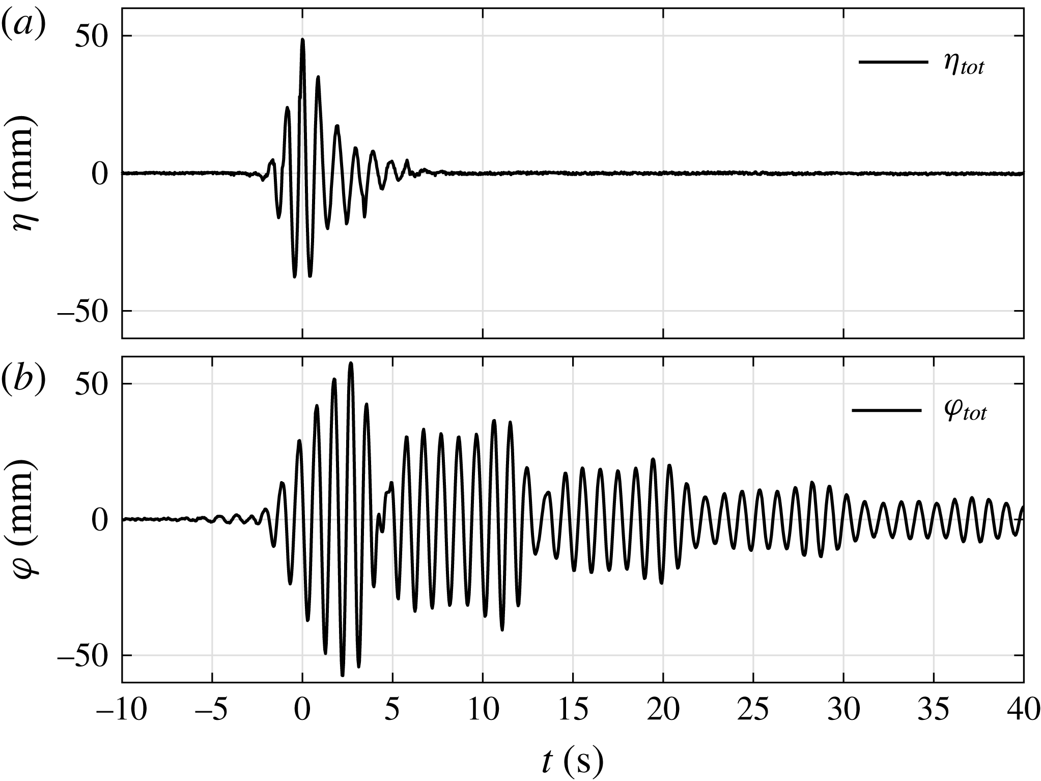
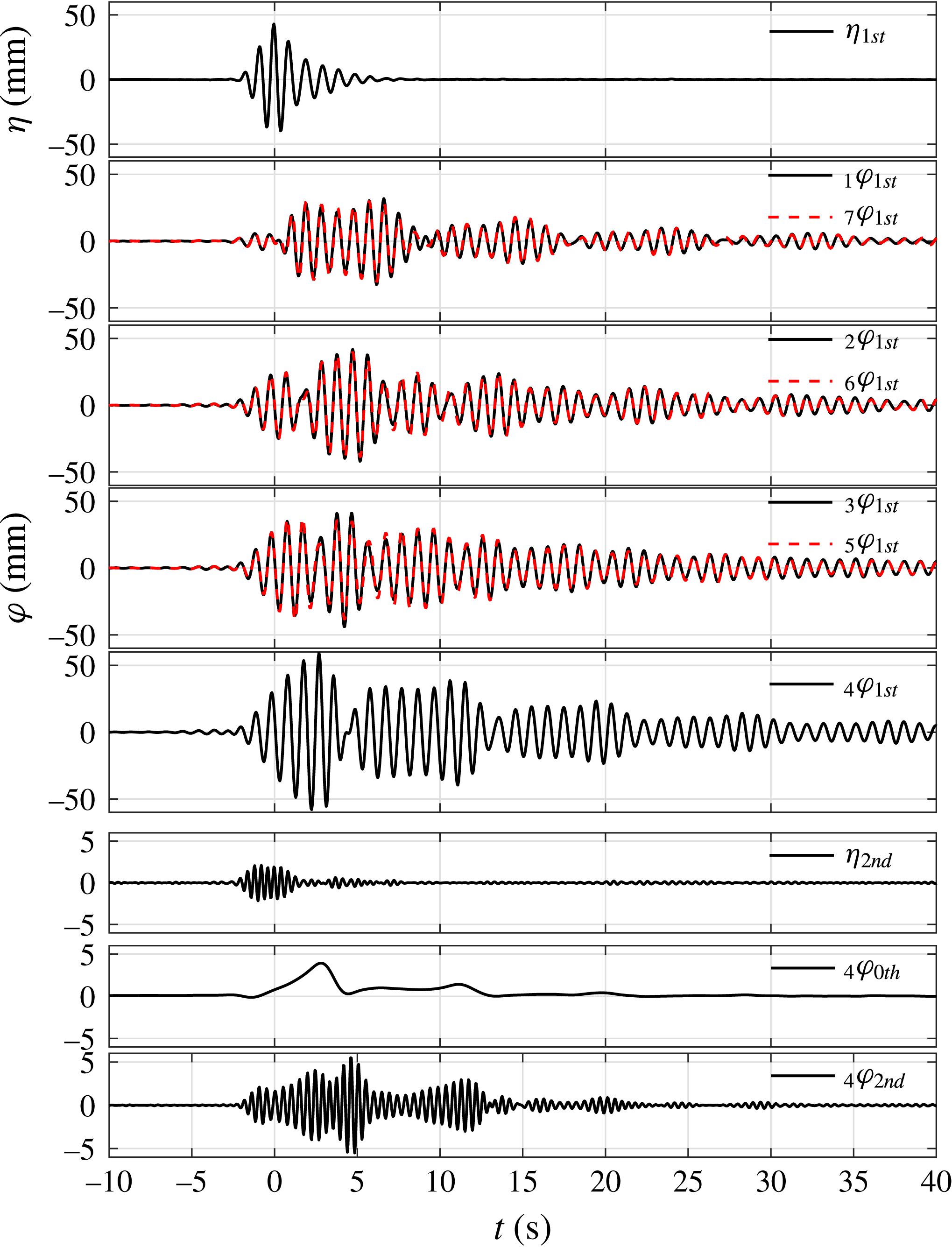
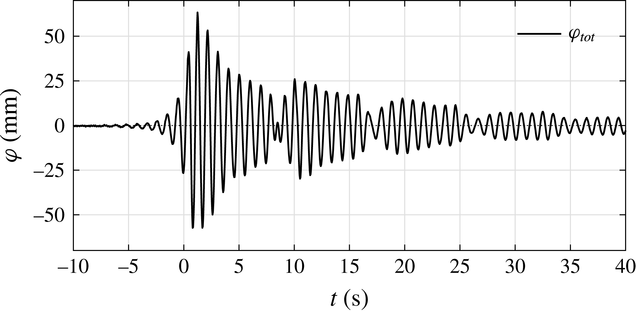
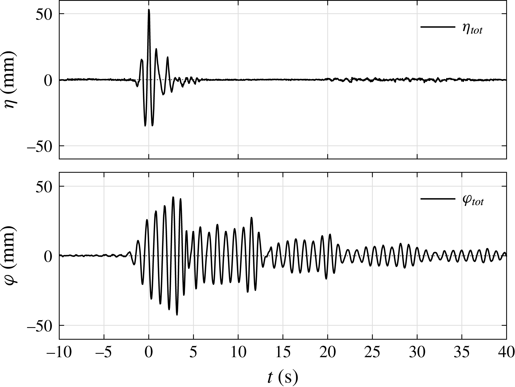
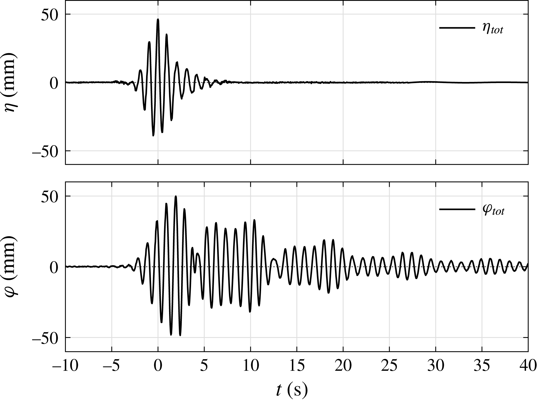
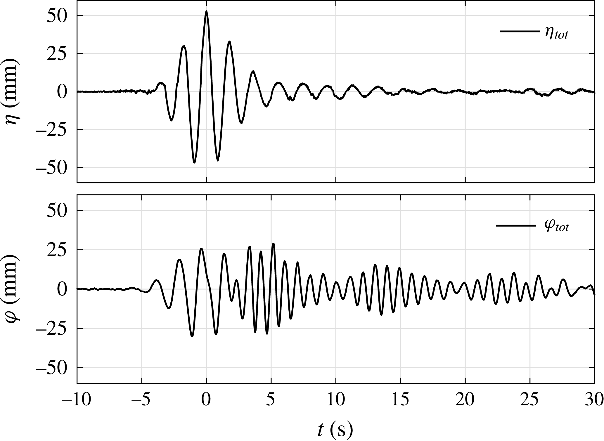
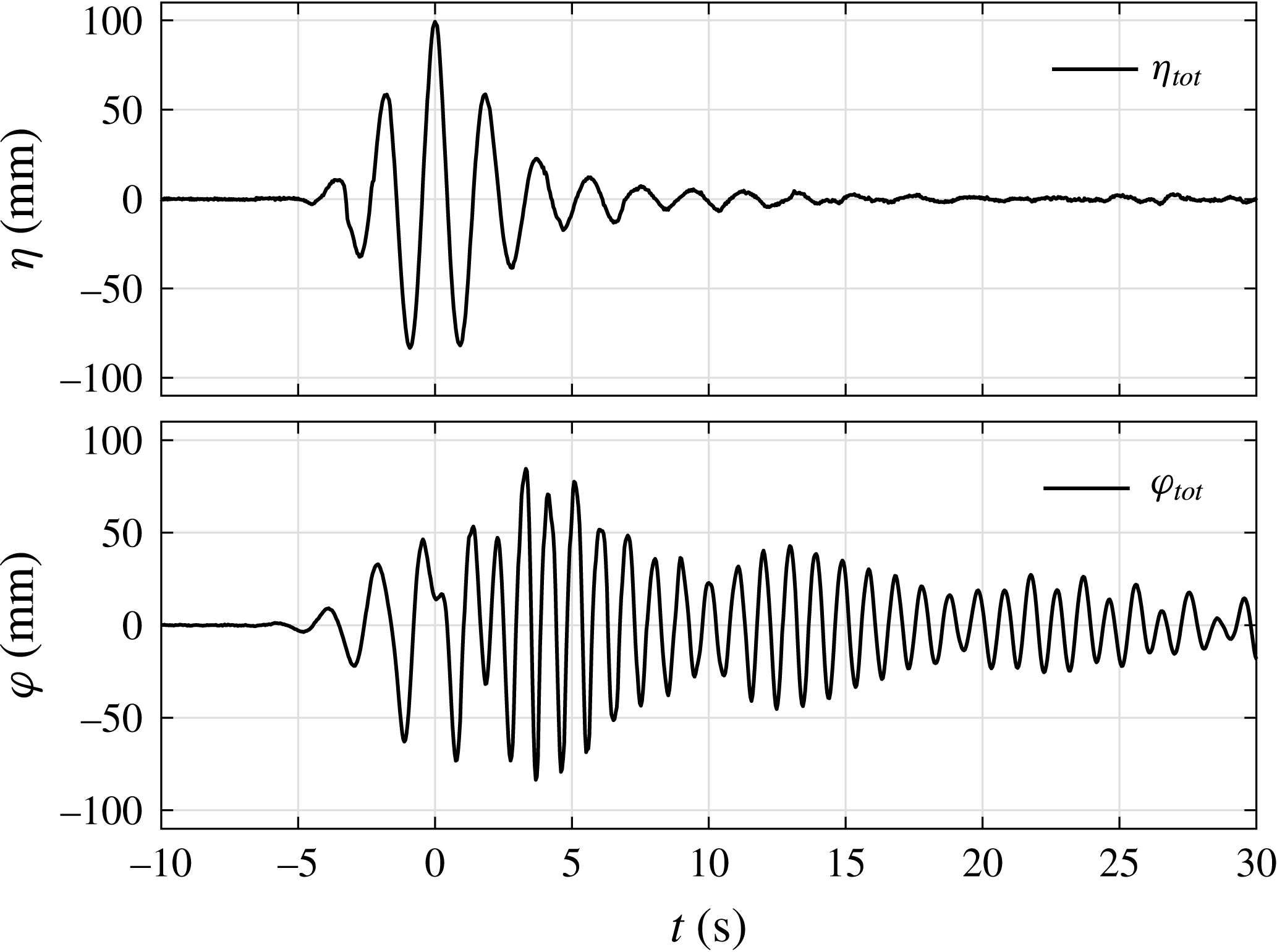
The free-surface elevations of the NewWave-type wave group (in the absence of the model) and the response at the centre of the gap (in the presence of the model) are plotted in figure 3. The focus time (at which maximum undisturbed surface elevation occurs) has been set as
 $t_{0}=0$
. The undisturbed incoming waves (
 $\unicode[STIX]{x1D702}$
) and the corresponding gap response free-surface elevations (
 $\unicode[STIX]{x1D711}$
) have been lined up in time. It is seen that the surface elevation in the gap takes time to build up and the gap resonant response shows a peak value slightly larger than the incoming wave, which then decays slowly, with a strong beating pattern.
Time histories of the free-surface elevations with (b) and without (a) the hull models in place for set I:
 $f_{P}=f_{m=1}$
and
 $\unicode[STIX]{x1D6FC}=50$
mm, beam sea, round bilge, Gaussian spectrum input. These time series were measured at the same position, i.e. the location of WG4 (the centre of the gap), and have been temporally aligned (focus time
 $t_{0}=0$
). Here,
 $\unicode[STIX]{x1D702}_{tot}$
is the total incident wave and
 $\unicode[STIX]{x1D711}_{tot}$
is the total surface elevation in the gap.

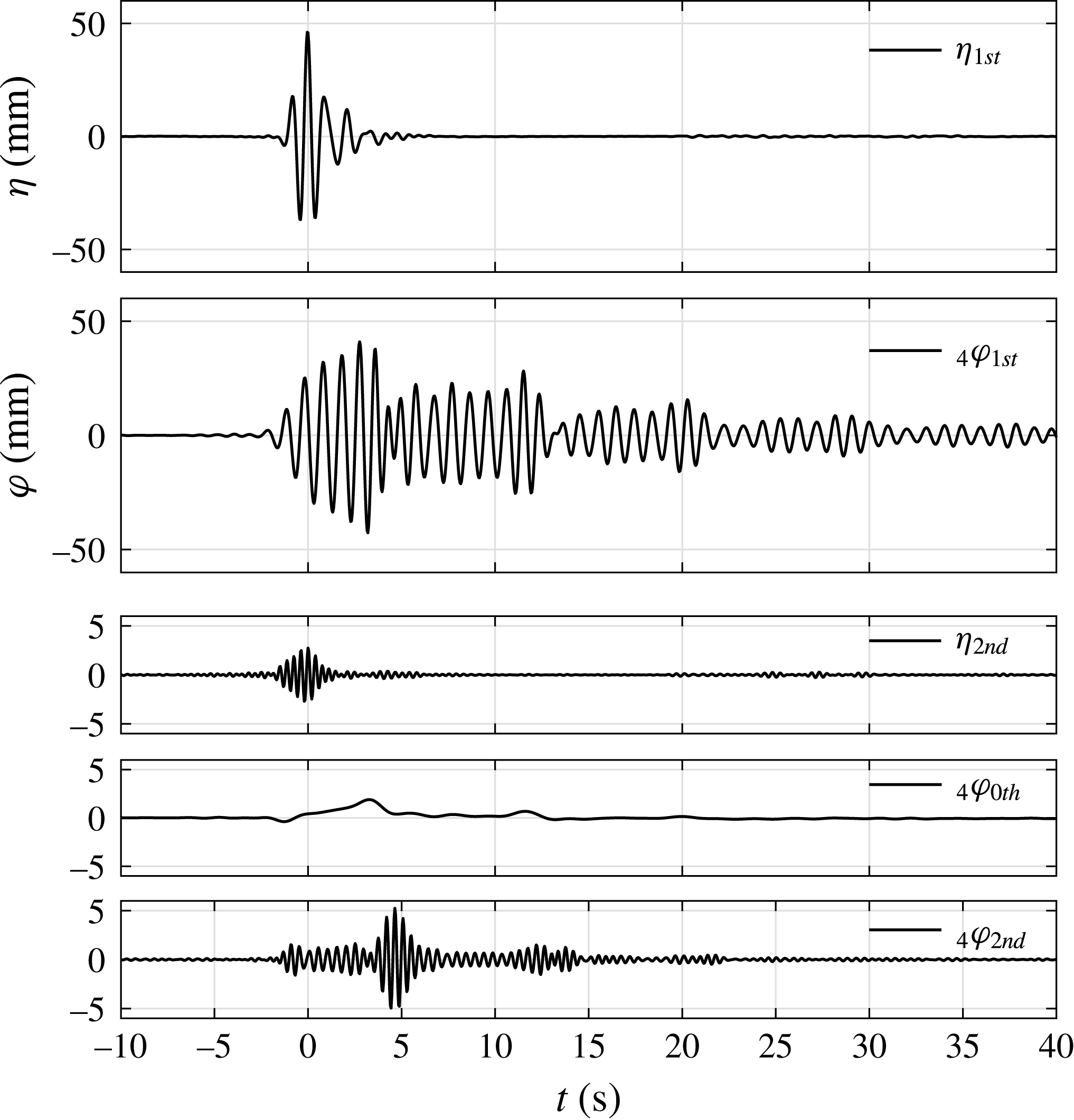
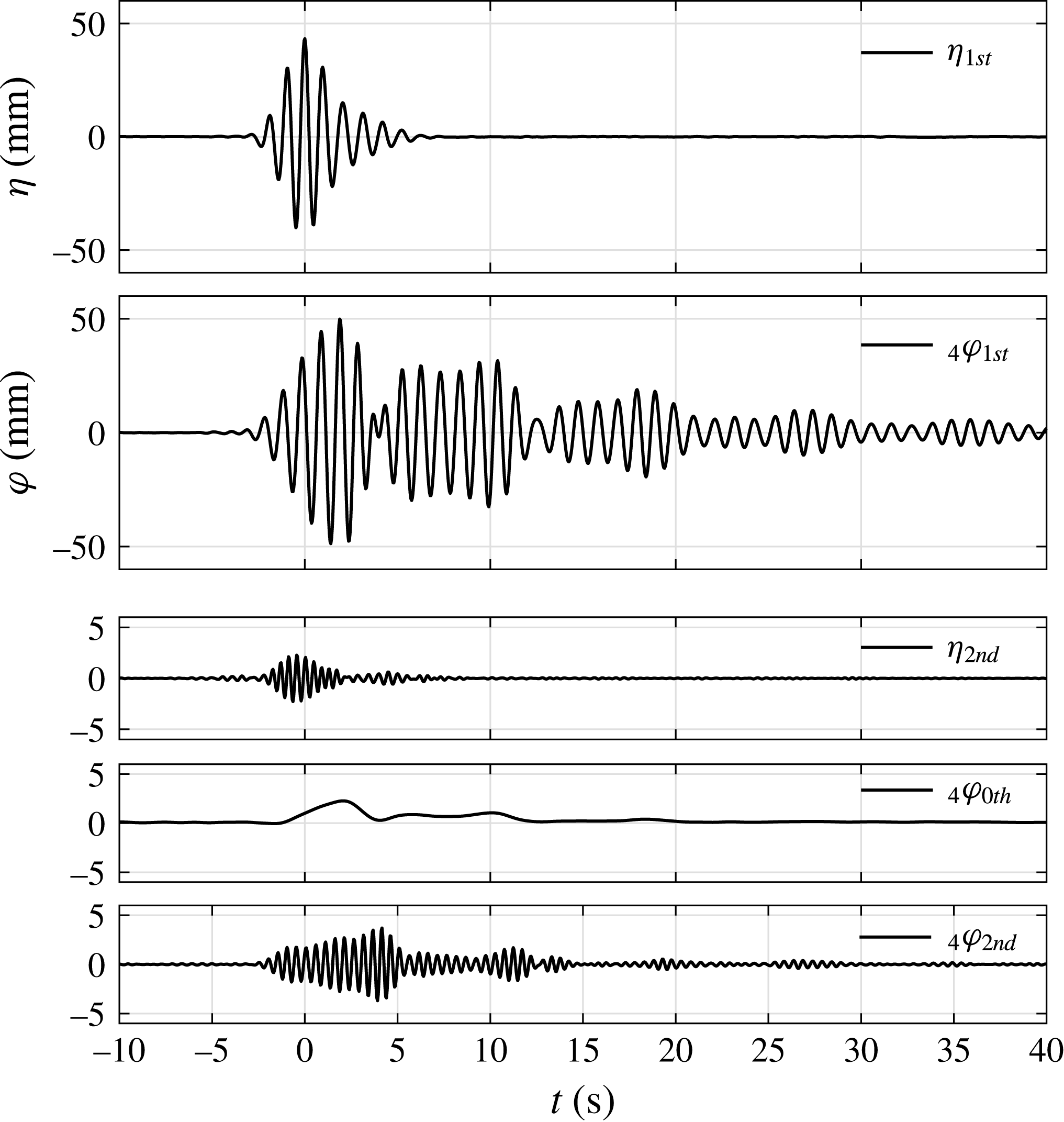
First and higher harmonic components of the incident wave group and gap response for set I:
 $f_{P}=f_{m=1}$
and
 $\unicode[STIX]{x1D6FC}=50$
mm, beam sea, round bilge, Gaussian spectrum input. The measurements in the symmetric WG pairs are plotted on the same axes for comparison. The left subscripts in the legend refer to the WG number and those on the right the harmonic components. Note the different vertical scales for the second harmonics.

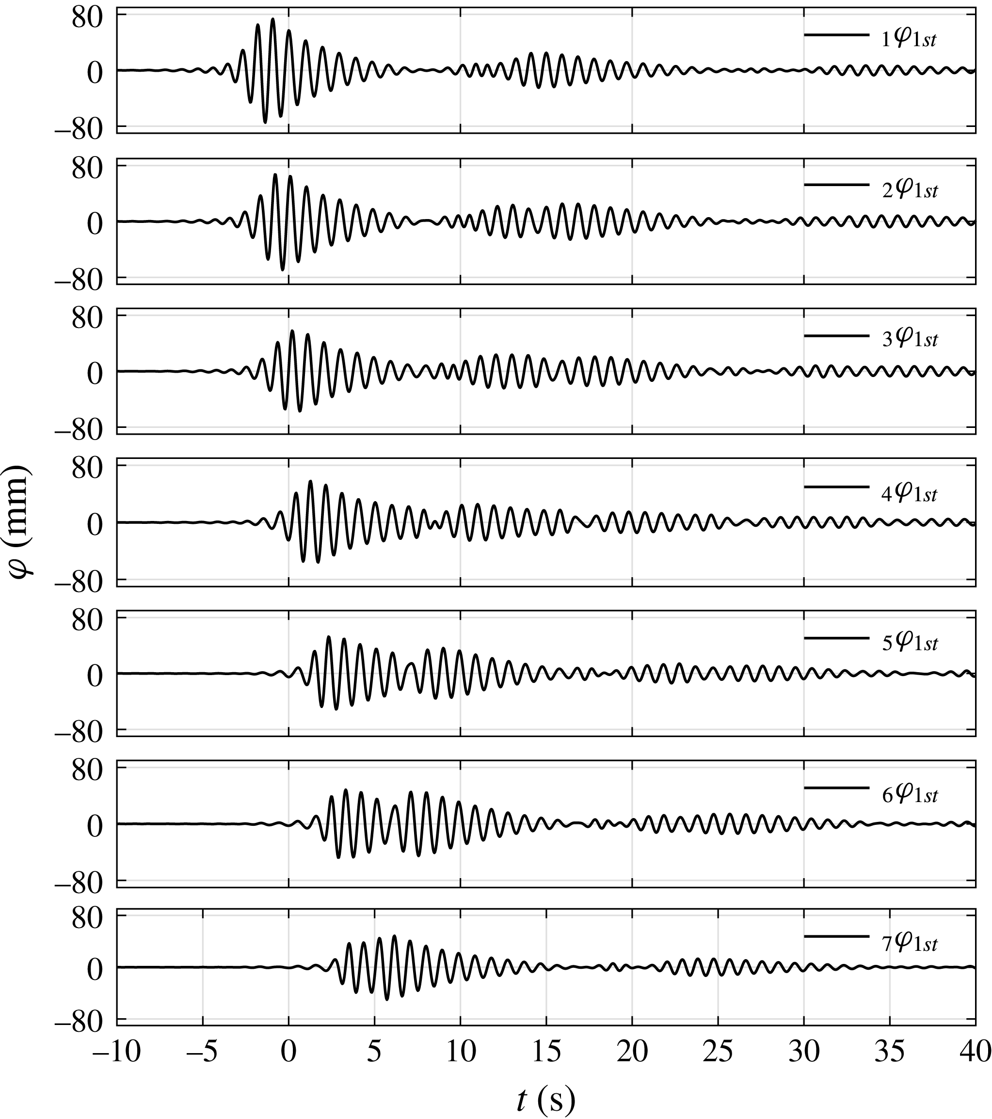
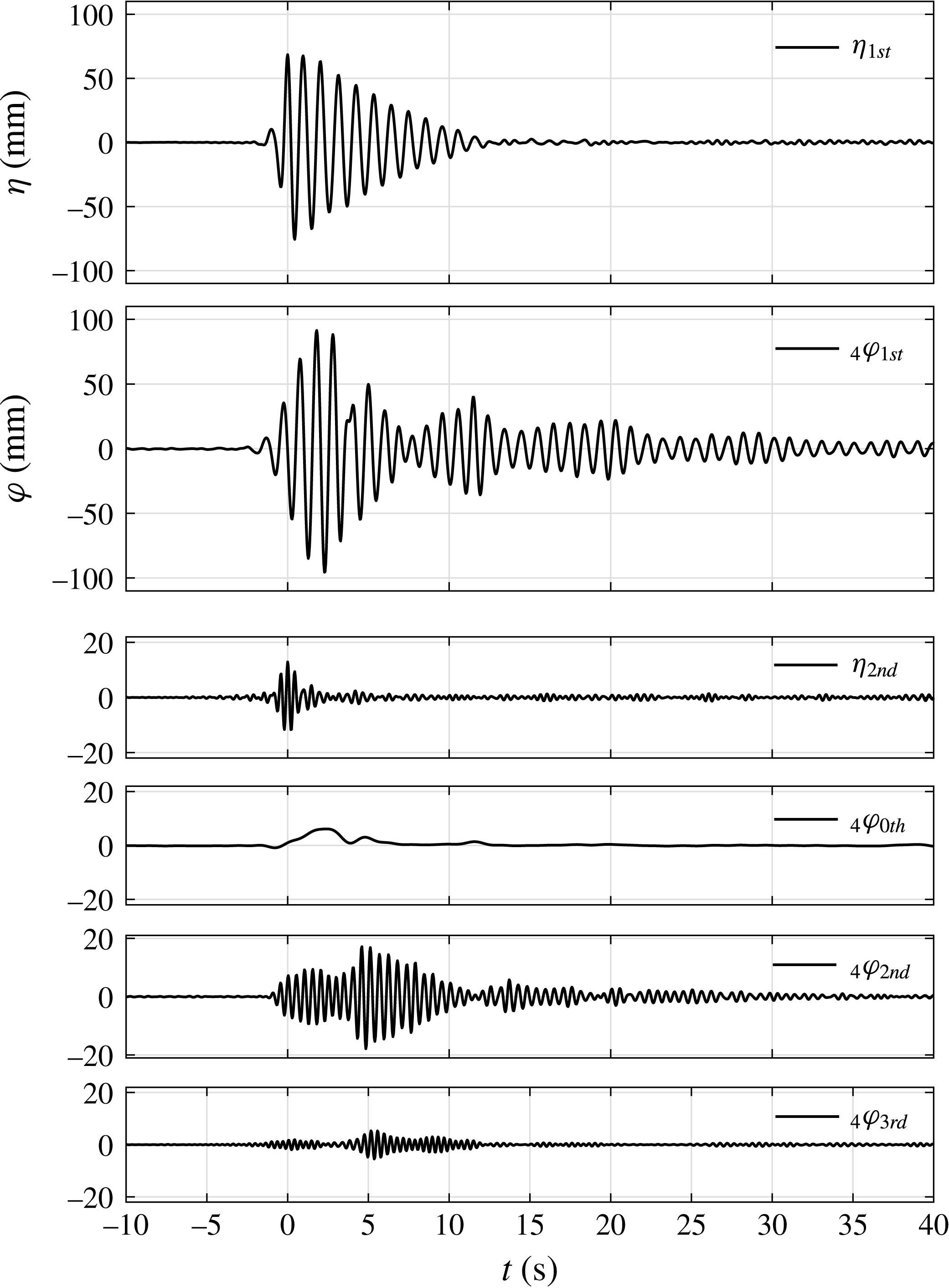
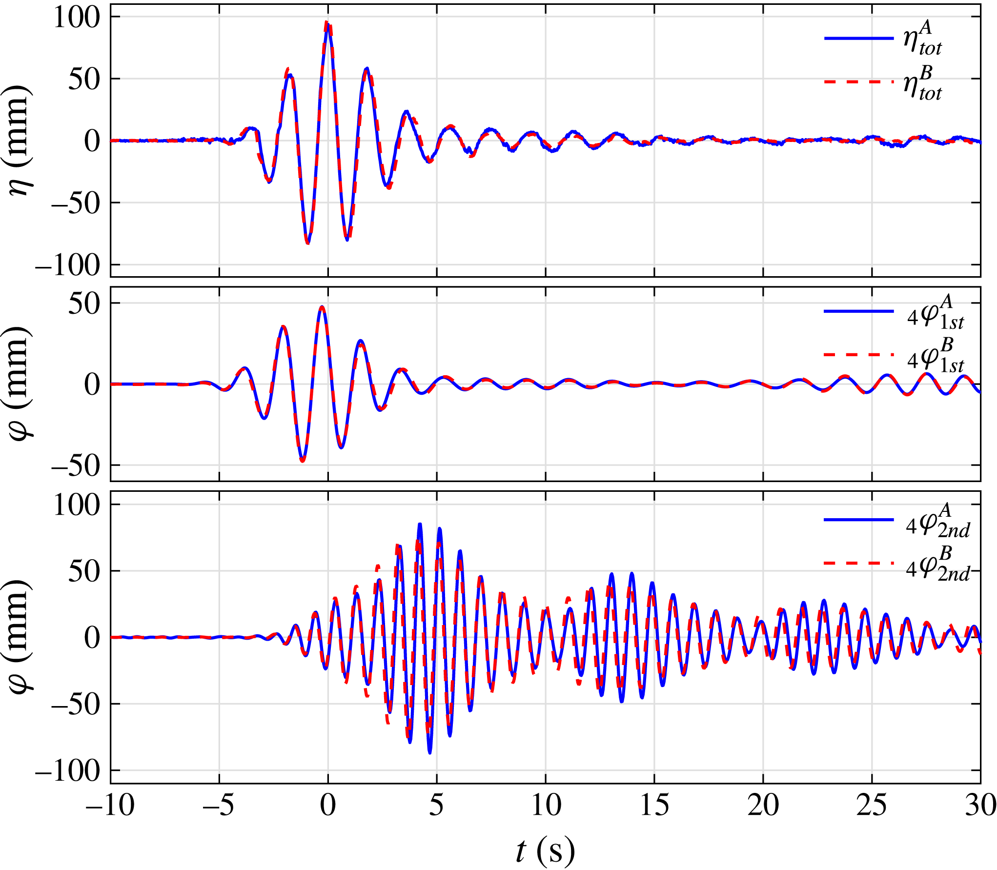
The four-phase combination method is then applied to the incoming NewWave groups and the corresponding gap responses respectively, to extract the harmonic components (see figure 4). The subscripts used for the individual component time histories are as follows:
 $_{a}\unicode[STIX]{x1D711}_{bth}$
refers to the time history from WG
 $a$
, as in figure 1, and the
 $b$
th frequency harmonic of the linear signal. Therefore, the bottom subplot in figure 4 was measured at WG4 and corresponds to the second harmonic (double frequency) term. The second harmonic component is significantly smaller than the first harmonic surface elevation for the incoming waves. The higher harmonics are invisible. For the corresponding gap resonant response, the second harmonic component is of significant size, while all of the other higher harmonics are negligible. In addition, the second-order difference harmonic which is the surface set-up (zeroth harmonic in figure 4) is observed.
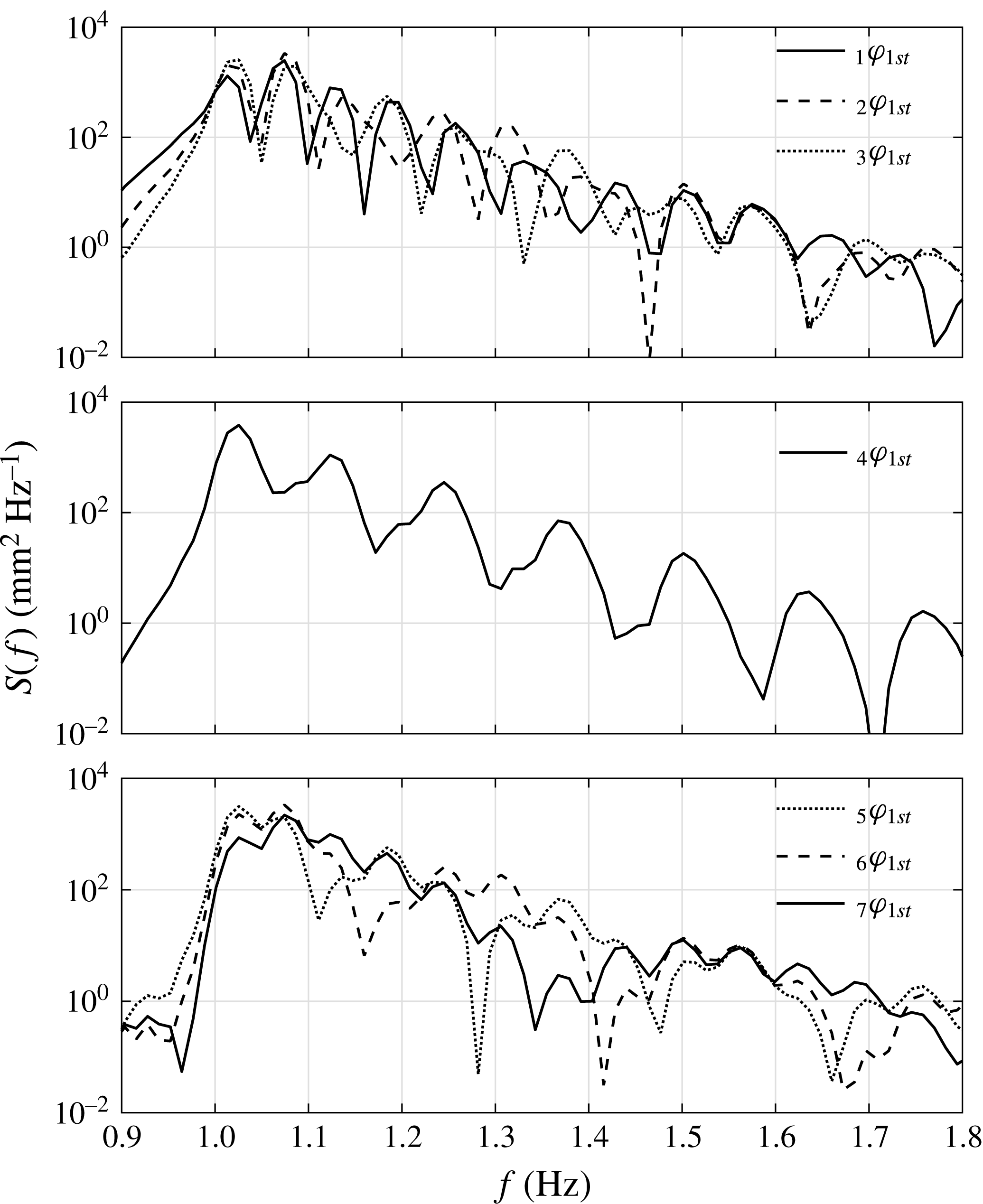
Spectra of the first harmonics of the gap responses in different locations for set I:
 $f_{P}=f_{m=1}$
and
 $\unicode[STIX]{x1D6FC}=50$
mm, beam sea, round bilge, Gaussian spectrum input. Here,
 $S(f)$
refers to the power spectrum and
 $f$
is the frequency. The left subscripts in the legend refer to the WG number and those on the right the harmonic components.

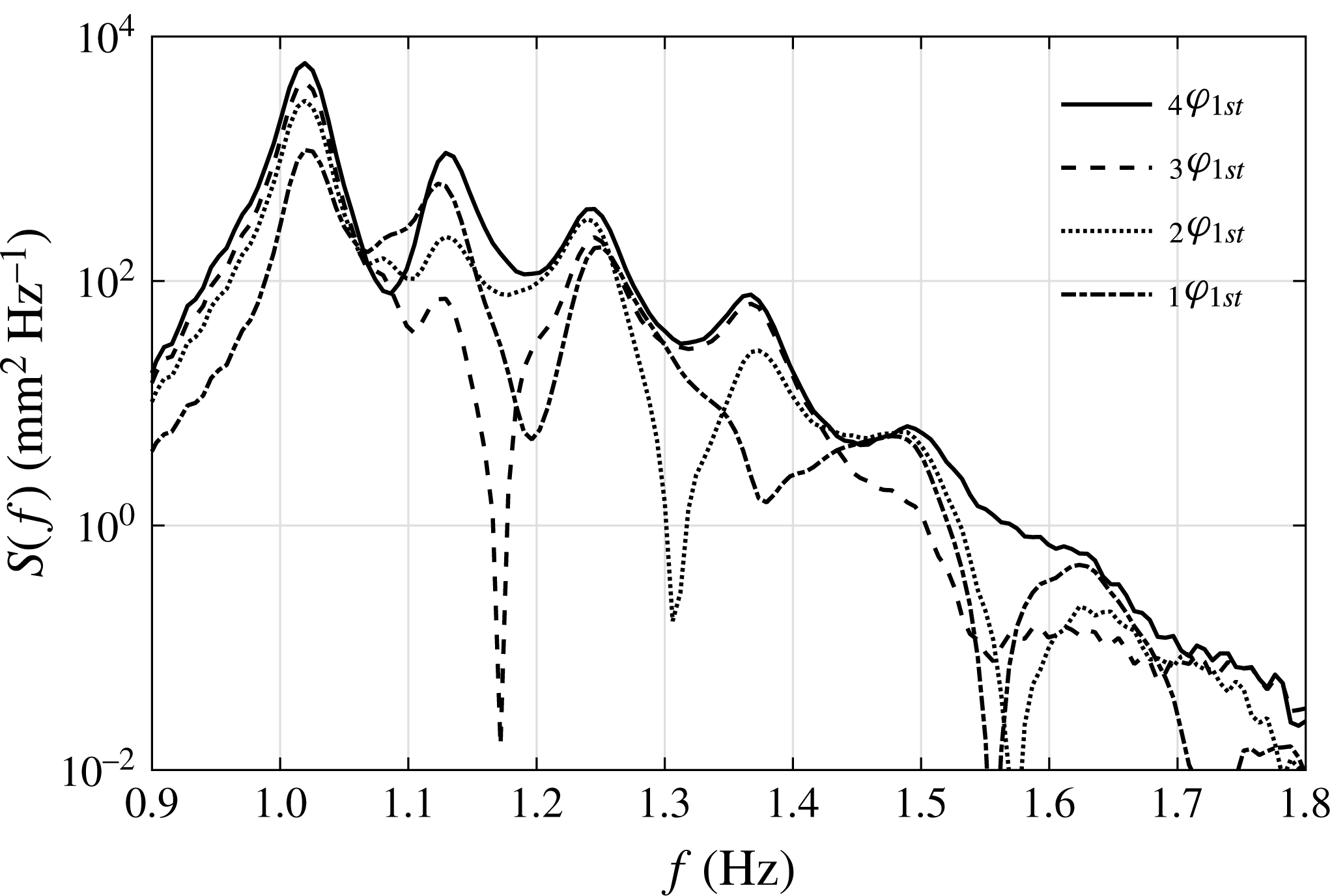
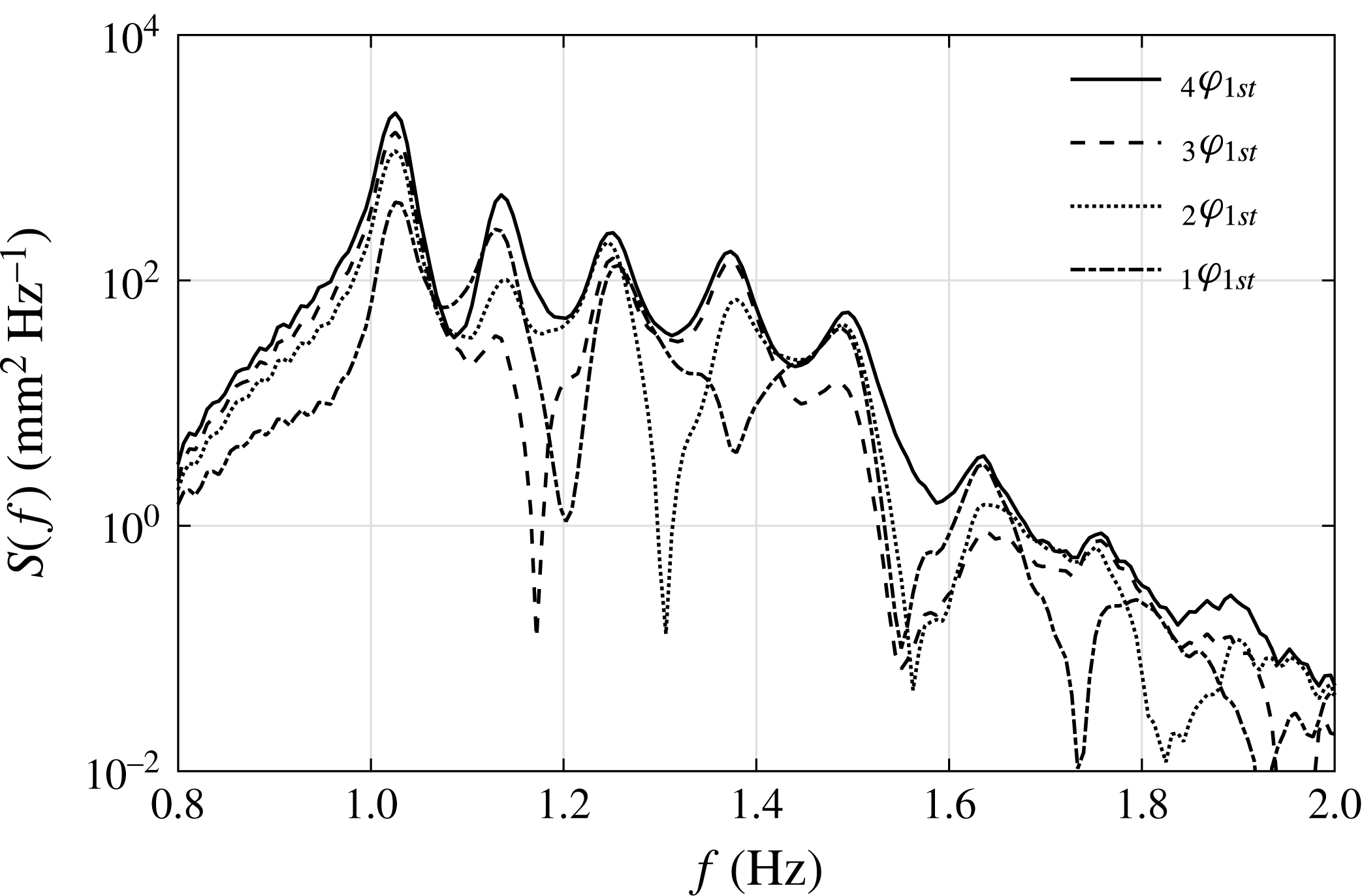
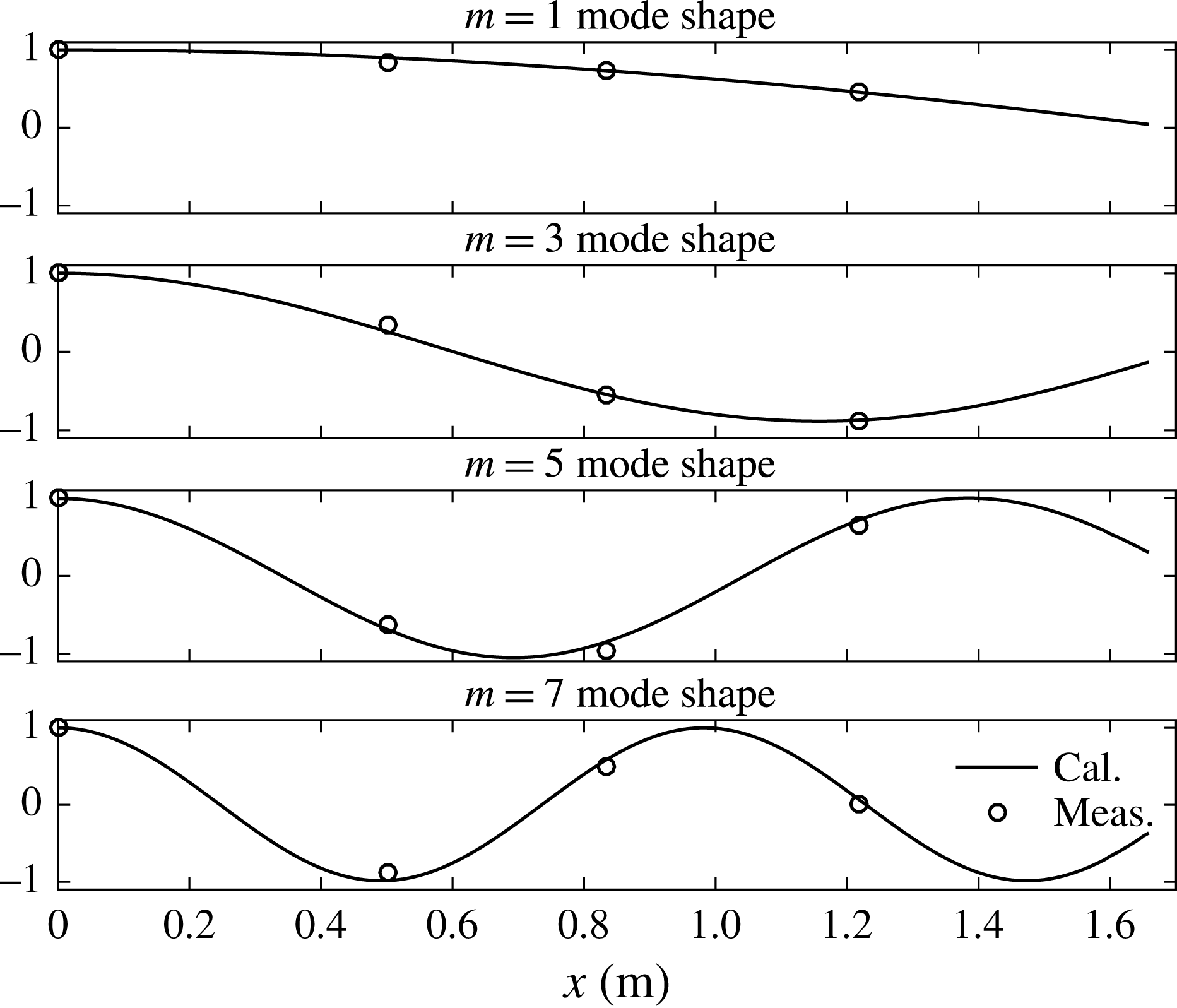
To study the variation of the resonant response in the gap, the four-phase combination is applied to the time histories from all WGs. All of the results for the symmetric WG pairs (see figure 4) show very good agreement, confirming the high-quality control of the experiments. From the time histories, we find the first mode resonant response decreasing as we go from the centre to the ends of the gap. Spectral analysis is performed to obtain the power spectral density of the linear resonant response (see figure 5), showing different spectral peaks. Table 2 compares the estimated frequencies of the peaks of the response spectra shown in figure 5 with linear potential theory predictions for each gap resonance mode (generated using the code DIFFRACT, e.g. Sun, Eatock Taylor & Taylor Reference Sun, Eatock Taylor and Taylor2015). Due to the symmetry of the experimental set-up and the incident wave field, only modes with odd numbers of half-wavelengths along the gap can be excited. We denote the numbers of half-wavelengths along the gap by
 $m$
. Very good agreement is observed. It is seen in figure 5 that the spectrum for WG4 shows a spectral peak at a frequency corresponding to the
 $m=3$
mode, while it is much reduced in the spectrum for WG3. This indicates that the location of WG3 is close to a node of the
 $m=3$
mode. Similarly, WG1 seems to be close to a node of the
 $m=7$
mode.
Frequencies for the odd modes of the gap resonant response. ‘Meas.’ stands for the measured data and ‘Cal.’ the simulations from DIFFRACT. The measured frequencies are the estimated frequencies of the peaks of the response spectra, while the calculated frequencies correspond to estimated frequencies of the peaks of the modulus of the complex transfer function for the free surface at the appropriate point.

Response spectra and phase of the cross-spectrum for WG1 with respect to WG4 (centre of the gap). Set I:
 $f_{P}=f_{m=1}$
and
 $\unicode[STIX]{x1D6FC}=50$
mm, beam sea, round bilge, Gaussian spectrum input.

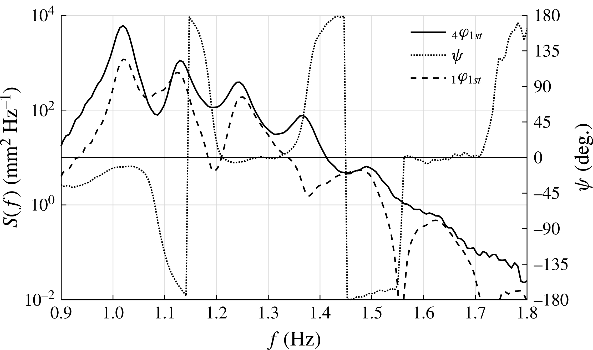
To derive the gap resonant mode information, complex cross-spectral analysis is conducted through
 $S_{xy}(f)=\int _{-\infty }^{\infty }R_{xy}(\unicode[STIX]{x1D70F})\text{e}^{-\text{i}2\unicode[STIX]{x03C0}f\unicode[STIX]{x1D70F}}\,\text{d}\unicode[STIX]{x1D70F}$
, where
 $R_{xy}(\unicode[STIX]{x1D70F})$
is the cross-correlation between the variables
 $x$
(WG1, 2 or 3) and
 $y$
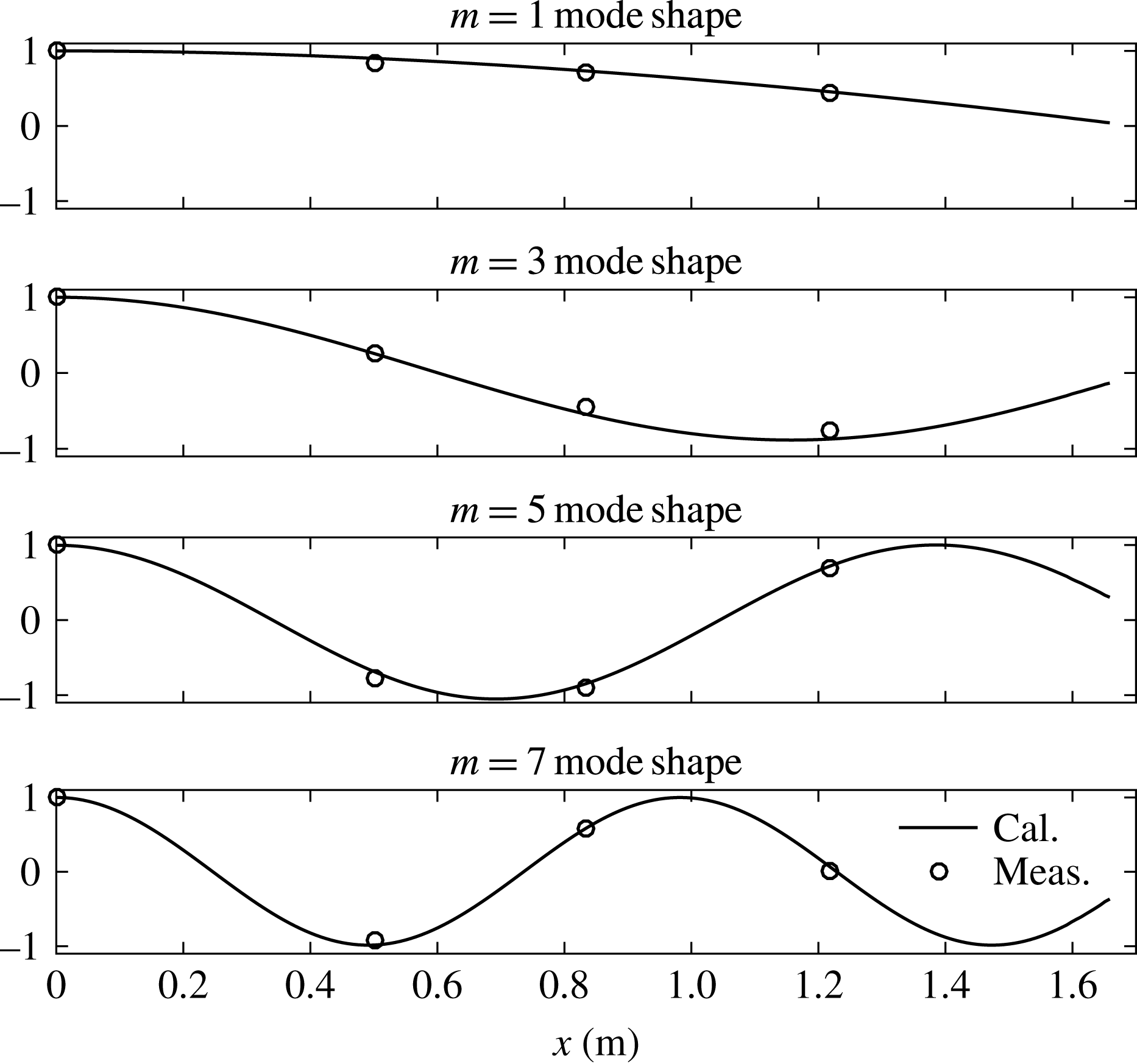
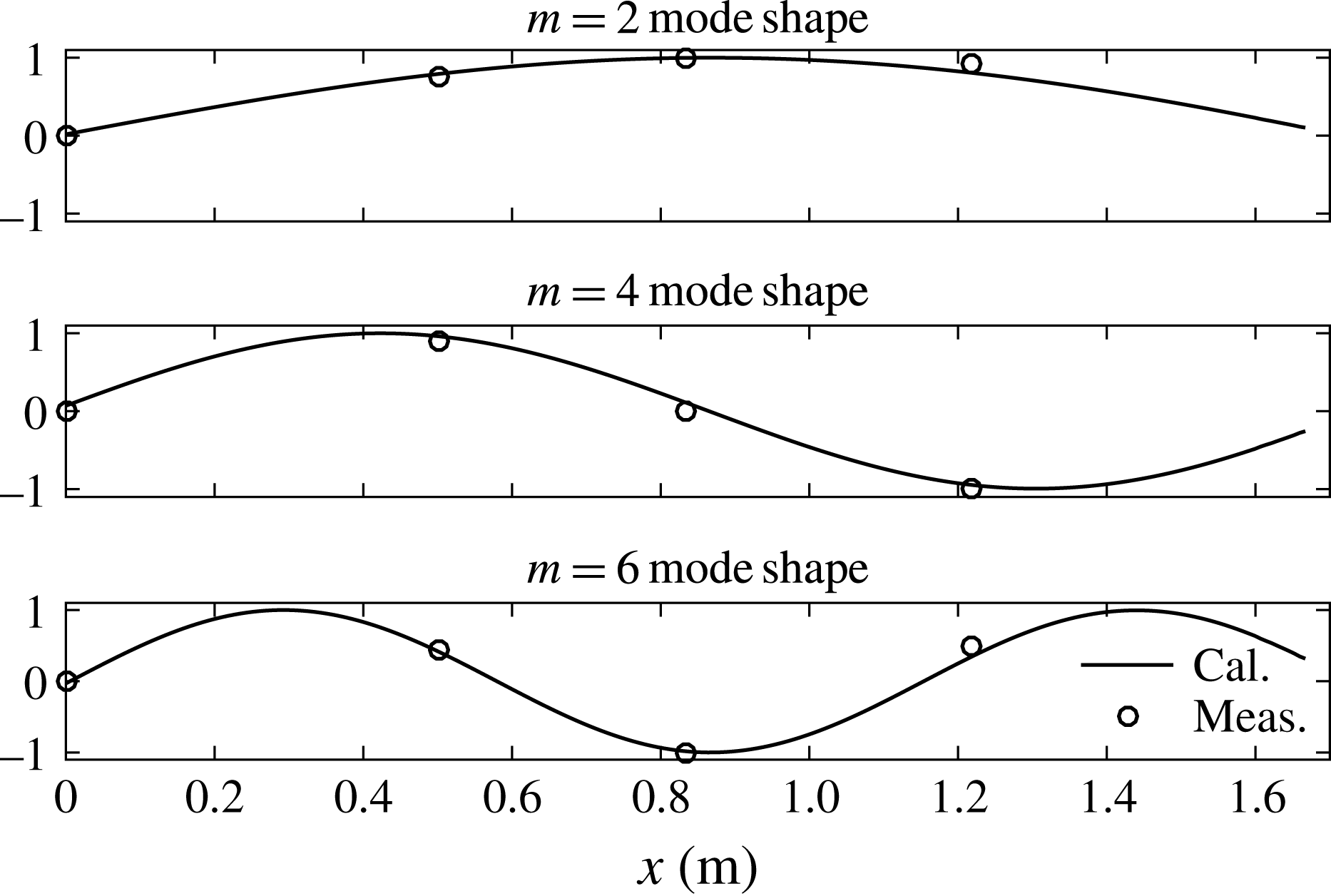
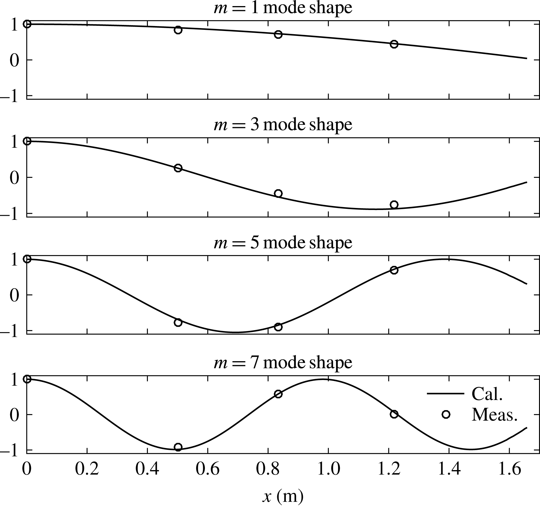
(WG4 in the centre of the gap). A representative cross-spectral result has been plotted in figure 6. The cross-spectral analysis gives the relative phase of the surface elevation at each WG (the relative amplitudes already being available from the amplitude spectra). These data are then compared with linear potential theory predictions of the mode shapes from DIFFRACT (Sun et al.
Reference Sun, Eatock Taylor and Taylor2015) (see figure 7). As shown in figure 7, the
 $m=1$
mode of the gap resonance has the same phase along the gap. This explains why the time histories (see figure 4) show the maximum surface elevation in the centre of the gap.
Mode shapes of the resonant response in the gap. Here,
 $x$
refers to the distance away from the midship point and the amplitudes have been normalised. ‘Cal.’ refers to the numerical simulations from DIFFRACT and ‘Meas.’ the measured data. Set I:
 $f_{P}=f_{m=1}$
and
 $\unicode[STIX]{x1D6FC}=50$
mm, beam sea, round bilge, Gaussian spectrum input.
The way in which the different modes with their respective shapes interact to produce the complex time-evolving pattern in the gap is shown in a movie in the online supplementary movies available at https://doi.org/10.1017/jfm.2016.824, based on the measured free surface (movie 1). Also in the online material is a short recording taken of the free surface within the gap around the location of WG4 (movie 2), the centre of the gap.
4.2 Heading effects – even modes
In the previous section, we only observe the odd modes of the gap resonant responses, due to the symmetry of the experimental set-up. In this section, a different orientation allows us to obtain both the odd and the even modes of the gap resonance. The incoming NewWave-type wave group is the same as that used in the ‘base case’, but the heading of the model has been changed so that the wave group approaches the model along the gap. To avoid repetition, we omit a plot of the incident wave. We only show the surface elevations of the gap resonant response for this case. The corresponding time series (see figure 8) of the gap resonant response show a beating pattern as well, but each beating pattern has a longer duration than in the beam sea cases (see figure 3). As in the base case, a movie illustrating the gap motion was generated for the head sea case and is given in the online supplementary material (movie 3).
Time histories of gap response from WG4 (centre of the gap) for set II:
 $f_{P}=f_{m=1}$
and
 $\unicode[STIX]{x1D6FC}=50$
mm, head sea, round bilge, Gaussian spectrum input.

First harmonic components of the gap resonant responses in different locations along the gap for set II:
 $f_{P}=f_{m=1}$
and
 $\unicode[STIX]{x1D6FC}=50$
mm, head sea, round bilge, Gaussian spectrum input; WG1 is the most upwave and WG7 the most downwave.

Second harmonic components of the gap resonant responses in different locations along the gap for set II:
 $f_{P}=f_{m=1}$
and
 $\unicode[STIX]{x1D6FC}=50$
mm, head sea, round bilge, Gaussian spectrum input.

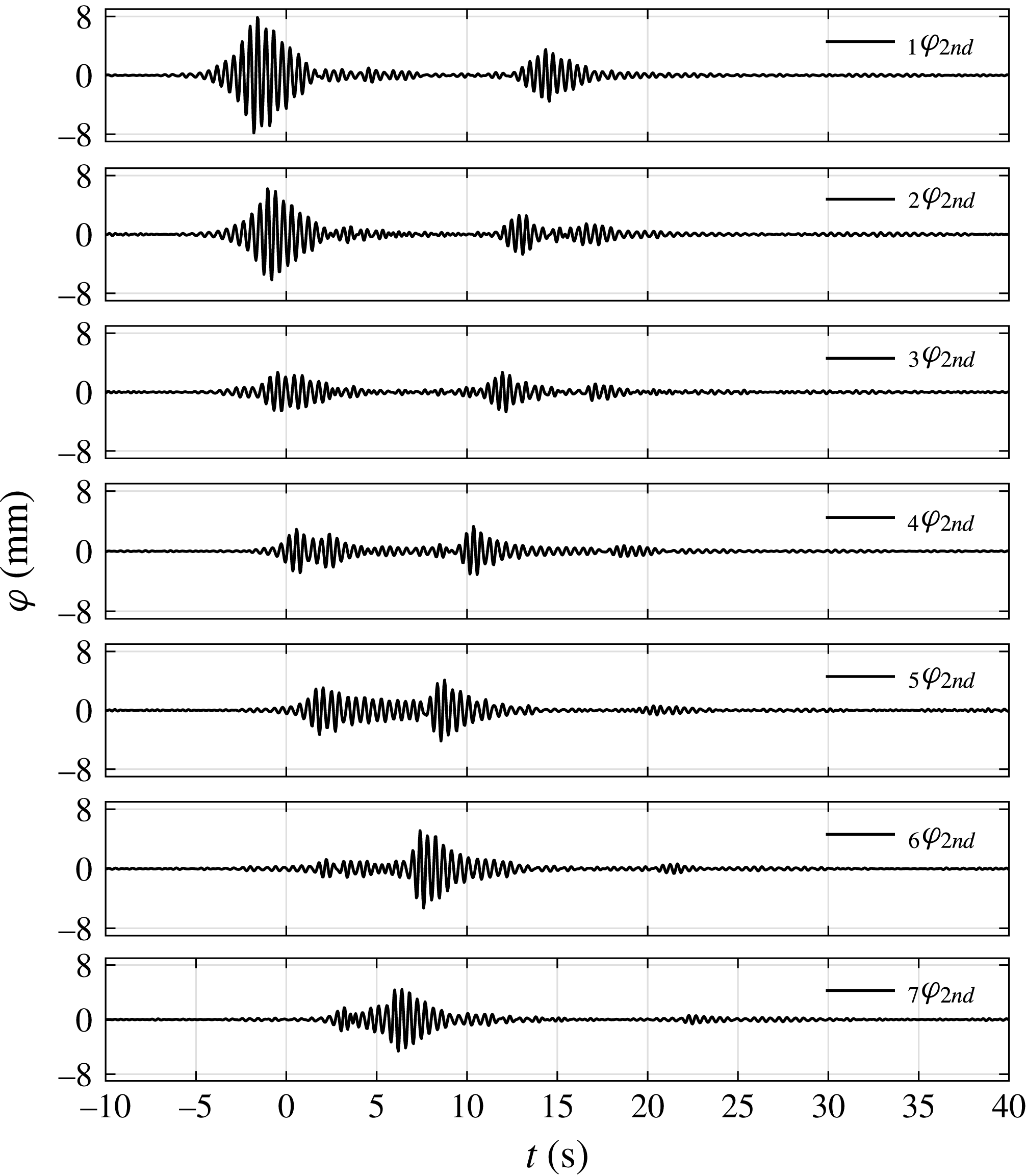
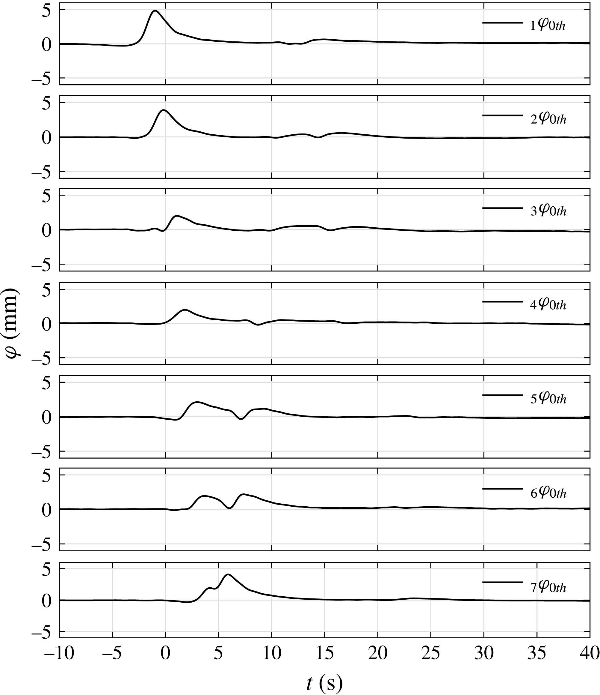
The harmonic components are extracted, and are plotted in figures 9–11, showing the variation of the resonant responses along the gap. Again, only the first two harmonic (and the zeroth harmonic) components are significant, and the other higher harmonics are invisible when plotted on the same vertical scale. It is worth pointing out that the second harmonic component is still very small compared with the first harmonic. Due to the loss of symmetry of the experimental set-up relative to the incoming waves, the signals measured by all of the WGs are different and can be usefully compared.
Zeroth harmonic components of the gap resonant responses in different locations along the gap for set II:
 $f_{P}=f_{m=1}$
and
 $\unicode[STIX]{x1D6FC}=50$
mm, head sea, round bilge, Gaussian spectrum input.

The first harmonic (linear) results (see figure 9) show that maximum amplification occurs at the upwave end of the gap and decreases towards the downwave end of the gap. At the downwave end of the gap, part of the gap resonance propagates back upwave, leading to a second pulse in the time histories. The second harmonic sum components (see figure 10) and the second harmonic difference components (see figure 11) show the same phenomenon. Each is like a propagating wave group in a channel, travelling down and reflecting at the ends of the gap.
Spectra of the first harmonic component of the gap resonant response in different locations along the gap for set II:
 $f_{P}=f_{m=1}$
and
 $\unicode[STIX]{x1D6FC}=50$
mm, head sea, round bilge, Gaussian spectrum input.

Illustration of the even mode shapes for the free surface in the gap. Here,
 $x$
refers to the distance away from midship and the amplitudes have been normalised. Set II:
 $f_{P}=f_{m=1}$
and
 $\unicode[STIX]{x1D6FC}=50$
mm, head sea, round bilge, Gaussian spectrum input.

As in table 2, but for frequencies of the even modes of the gap resonant response.

Due to the asymmetry of the input waves along the gap, antisymmetric modes of the gap resonant responses (with even numbers of half-wavelengths along the gap) are excited, in addition to the odd modes observed in set I. The measured frequencies of the even modes of the gap resonance agree well with predictions, as shown in table 3. Spectra of the surface elevations in the gap are plotted in figure 12 for different WGs. WG4 (the central wave gauge) is located at a node of all even modes, so there are no spectral peaks for these modes. WG2 is located approximately at a node of the
 $m=4$
and higher modes. To illustrate the even mode shapes of the gap resonant response, we plotted the (admittedly rather coarsely sampled) measurements in space against the predicted even mode shapes from linear potential theory (see figure 13), showing reasonable agreement.
4.3 Bandwidth effect: wave groups based on a Gaussian spectrum versus a Pierson–Moskowitz spectrum
A Gaussian spectrum may be a good model for swell waves; broadbanded spectra associated with wind waves are also common. To investigate the effect of spectral bandwidth, we measured the gap responses under excitation by a NewWave associated with a Pierson–Moskowitz (PM) spectrum, with the same peak frequency as in set I. The incident NewWave group profile associated with the (broader) PM spectrum (see figure 14) is more compact than that (see figure 3) related to the (narrower) Gaussian spectrum. The shorter duration of the PM NewWave group leads to a smaller gap response as there is less time for the resonance to build up. The extracted harmonics in figure 15 provide clearer results illustrating this. As expected, more spectral response peaks are excited by the more broadbanded input from the PM spectrum (see figure 16).
As in figure 3, but for set III:
 $f_{P}=f_{m=1}$
and
 $\unicode[STIX]{x1D6FC}=50$
mm, beam sea, round bilge, PM spectrum input.

First and higher harmonic components of the incident wave group and gap response from WG4 (centre of the gap) for set III:
 $f_{P}=f_{m=1}$
and
 $\unicode[STIX]{x1D6FC}=50$
mm, beam sea, round bilge, PM spectrum input. Note the different vertical scales for the second harmonics.

As in figure 5, but for set III:
 $f_{P}=f_{m=1}$
and
 $\unicode[STIX]{x1D6FC}=50$
mm, beam sea, round bilge, PM spectrum input.

4.4 Bilge shape effect – round corner versus square corner
To investigate the effect of bilge shape, another set of NewWave group experiments is carried out with the round corners of the two fixed hulls replaced with square corners. This alters the frequencies of the gap resonant modes, with the first mode frequency now measured to be
 $f_{m=1}=0.945$
Hz. The incoming NewWave-type wave group is derived from a Gaussian spectrum with parameters
 $f_{P}=f_{m=1}$
and
 $\unicode[STIX]{x1D6FC}=50$
mm.
As in figure 3, but for set IV:
 $f_{P}=f_{m=1}$
and
 $\unicode[STIX]{x1D6FC}=50$
mm, beam sea, square bilge, Gaussian spectrum input.

As in figure 15, but for set IV:
 $f_{P}=f_{m=1}$
and
 $\unicode[STIX]{x1D6FC}=50$
mm, beam sea, square bilge, Gaussian spectrum input.

With square corners, the gap resonant response (see figure 17) is smaller than that obtained with round corners (see figure 3). Again, only the linear and second harmonics are excited (see figure 18), and no higher (than second) harmonics can be observed for the gap resonant response for this case with square corners.
4.5 Nonlinearity and wave breaking effects
The effect of wave steepness on gap response is of interest. Hence, a wave group with the same peak period and set-up as set I, but with the amplitude doubled to
 $\unicode[STIX]{x1D6FC}=100$
mm (
 $k_{P}\unicode[STIX]{x1D6FC}=0.42$
), was investigated. Unfortunately, but not surprisingly, this wave group became so steep that breaking occurred as it propagated down the tank. With the breaking observed, the linear steepness obtained from the four-phase combination at the position of the middle of the gap but without the models in place is
 $k_{P}\unicode[STIX]{x1D6FC}_{1st}=0.29$
.
As in figure 3, but for set V:
 $f_{P}=f_{m=1}$
and
 $\unicode[STIX]{x1D6FC}=100$
mm, beam sea, round bilge, Gaussian spectrum input.

As addressed by Adcock, Taylor & Gibbs (Reference Adcock, Taylor and Gibbs2016) and the extensive earlier literature referenced therein, nonlinearity (third-order wave–wave interactions) leads to significant changes to the shape of a focused wave group – relative to linear evolution, nonlinear groups become taller and narrower, with the largest wave in the group moving towards the front of the wave group. The nonlinear physics will drive a local increase in the bandwidth and further generate a very sharp spike at the front of the envelope peak. The shape of the incident NewWave group is plotted in figure 19, showing significant asymmetry relative to the focus position. As a consequence of the nonlinear evolution, the initial linear spectrum of focused wave groups will broaden and be modified as the wave group focuses with a downshift of the spectral peak. We note that, in the absence of wave breaking, these group changes would be close to identical for our four-phase groups. Each of the
 $90^{\circ }$
,
 $180^{\circ }$
and
 $270^{\circ }$
phase shifts relative to the
 $0^{\circ }$
case was carried out despite the significant change in group properties caused by breaking.
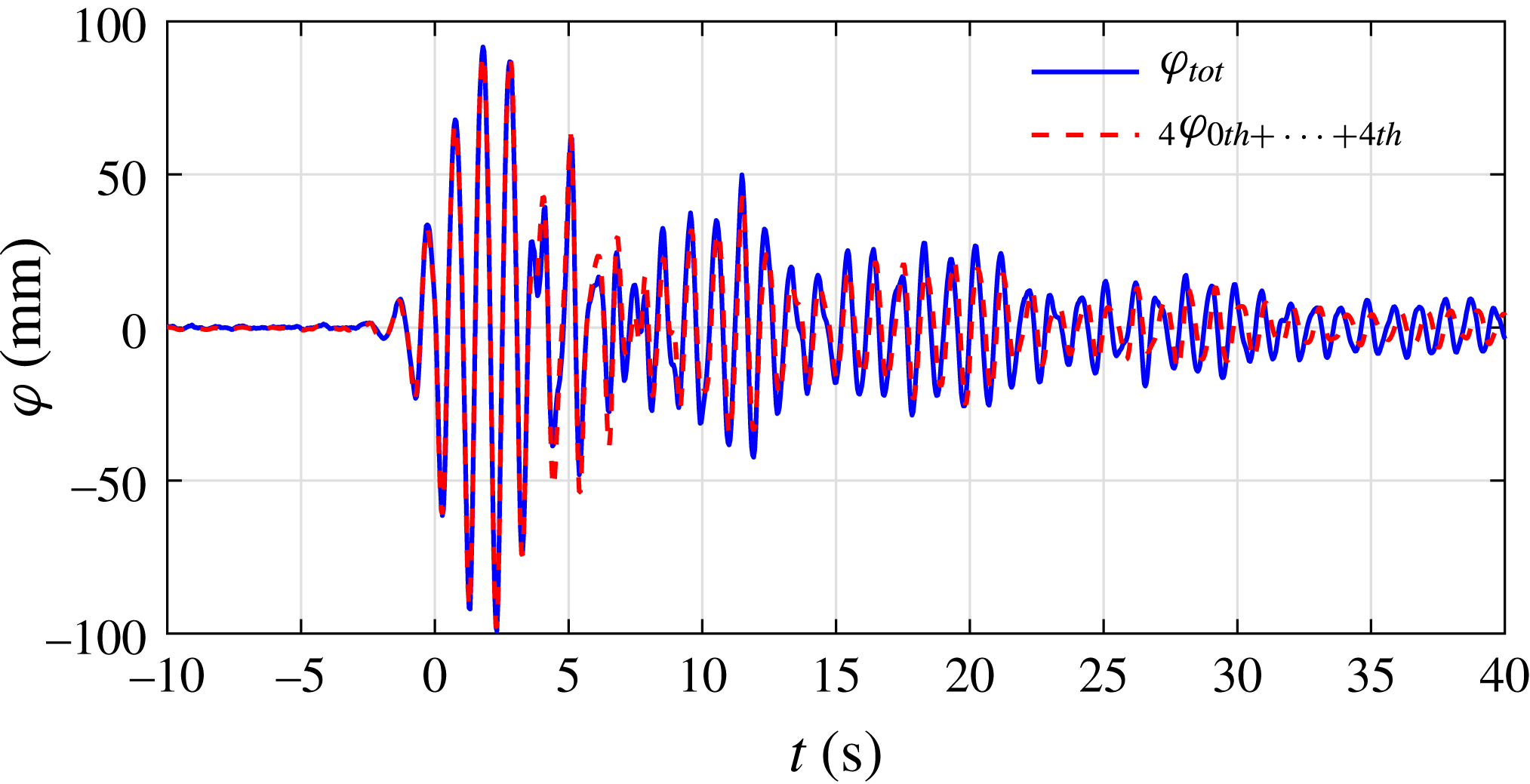
The four-phase combination results (see figure 20) show a second harmonic for the incident NewWave group and obvious second harmonics in the corresponding gap resonant responses. However, on the scale of the figure, the third harmonic is just visible but very small. Wave breaking disrupts the four-phase decomposition to a certain degree, and as a consequence, the sum of the first four harmonics does not completely recover the total signal (see figure 21). However, the four-phase combination methodology still works quite well for the first 5 s or so of the time history (see figure 21), where the linear response dominates.
As in figure 15, but for set V:
 $f_{P}=f_{m=1}$
and
 $\unicode[STIX]{x1D6FC}=100$
mm, beam sea, round bilge, Gaussian spectrum input.

Comparison of the original total response signal and the sum of the harmonic components from WG4 for set V:
 $f_{P}=f_{m=1}$
and
 $\unicode[STIX]{x1D6FC}=100$
mm, beam sea, round bilge, Gaussian spectrum input.

Spectra of the first two harmonic components for the incoming waves and the corresponding gap responses from WG4 for set V:
 $f_{P}=f_{m=1}$
and
 $\unicode[STIX]{x1D6FC}=100$
mm, beam sea, round bilge, Gaussian spectrum input.

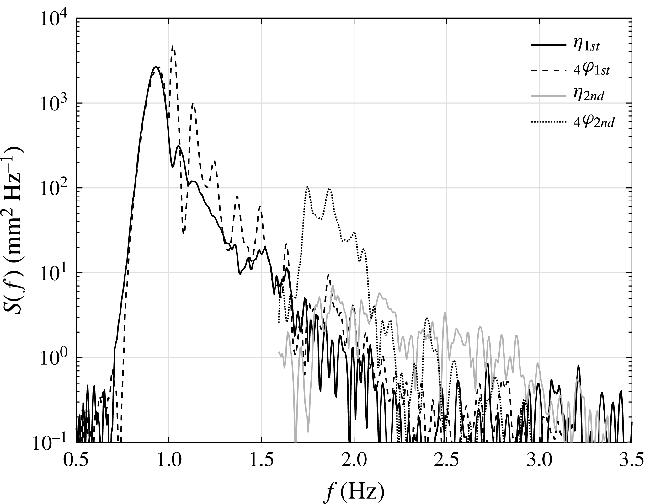
To identify the effects of nonlinearity and wave breaking, spectral analyses have been conducted for the linear and second harmonic signals, and the results are shown in figure 22. It is clear that the first harmonic of the gap response exhibits a spectral peak at a frequency lower than that of the first mode gap resonance. This frequency is in fact very close to the measured peak frequency of the incident NewWave group. We note that the peak frequency of the second harmonic signal is double the peak frequency for the incident NewWave group at approximately 1.8 Hz. This frequency does not correspond directly to a mode of the gap resonant response, though it appears that some higher modes may be excited. However, this observation led to the suggestion that the gap resonant response might be significantly driven by incident waves with half the frequency of the
 $m=1$
mode. This will be of practical concern later, because at full scale the first gap mode is at 7.5 s, where there is less energy than at 15 s in typical oceanic swell from distant severe storms.
4.6 Higher harmonics driven by half-frequency input
With the same experimental set-up as the ‘base case’, but halving the peak frequency (
 $f_{P}=1/2f_{m=1}$
), we investigated the harmonic structure of the surface motion in the gap. The measured time histories are shown in figure 23. With the model in place, the wave field reflected by the hull model will be rereflected by the wavemakers and back to the model. As a consequence, the exploitable duration of the measurements is twice the distance from the model to the wavemakers divided by the group velocity (the model is closer to the wavemakers than the wave absorbers in this study). In this long-wave half-frequency case, the group velocity is larger and thus we can observe some disturbance in the gap resonant response after
 $t=20$
s. The time history of the gap resonant response (see figure 23) shows a clear beating pattern. At the very beginning, the free surface in the gap oscillates with the same frequency as the incident waves. When the incident waves have passed, the free surface in the gap starts to oscillate at higher frequencies, which are a combination of different gap resonance modes.
As in figure 3, but for set VIA:
 $f_{P}=1/2f_{m=1}$
and
 $\unicode[STIX]{x1D6FC}=50$
mm, beam sea, round bilge, Gaussian spectrum input.

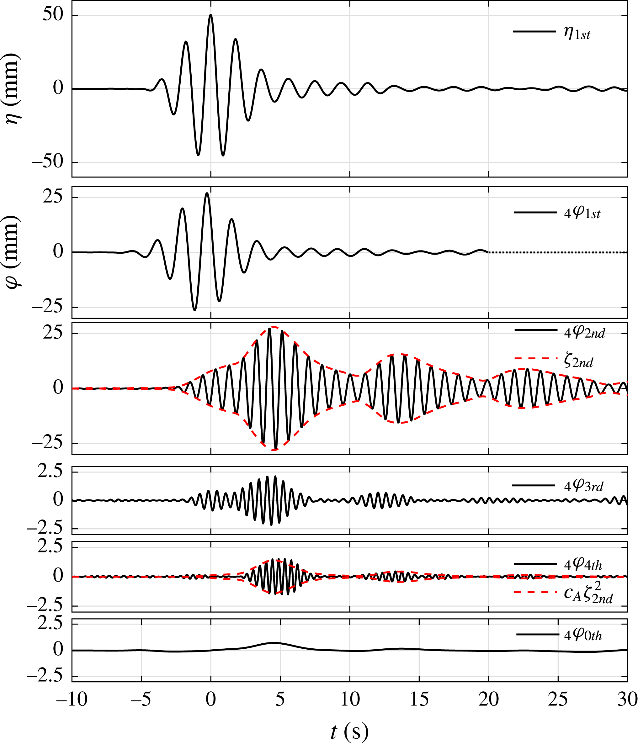
The four-phase combination results (see figure 24) show significant higher harmonics in the gap resonant responses. The second harmonic with the model in place is now slightly larger than the linear component, although there is negligible second harmonic for the incident NewWave group. Higher harmonics (e.g. the third and fourth harmonics) are also visible. The beating frequency in the second harmonic time history (see figure 24) is approximately 0.1 Hz, which is governed by the
 $m=1$
(
 $f_{m=1}=1.02$
Hz) and
 $m=3$
(
 $f_{m=3}=1.12$
Hz) modes. The fourth harmonic component of the gap resonance seems to be driven by the second harmonic component, if we note the very similar shape. To support this, we calculated the envelope of the second harmonic component from
 $\unicode[STIX]{x1D701}=\sqrt{\unicode[STIX]{x1D711}^{2}+\unicode[STIX]{x1D711}_{H}^{2}}$
, where
 $\unicode[STIX]{x1D711}_{H}$
is the Hilbert transform of the harmonic component. The envelope of the second harmonic component is plotted on top of its time history. The squared envelope of the second harmonic component is then scaled to match the amplitude of the fourth harmonic time history. The remarkably good match of the envelope shape between the scaled squared envelope of the second harmonic and the fourth harmonic time series indicates how the fourth harmonic ‘follows’, or is bound to, the second harmonic component.
As in figure 15, but for set VIA:
 $f_{P}=1/2f_{m=1}$
and
 $\unicode[STIX]{x1D6FC}=50$
mm, beam sea, round bilge, Gaussian spectrum input. Here,
 $\unicode[STIX]{x1D701}_{2nd}$
stands for the envelope of the second harmonic and
 $c_{A}\unicode[STIX]{x1D701}_{2nd}^{2}$
is a squared
 $\unicode[STIX]{x1D701}_{2nd}$
scaled by factor
 $c_{A}$
.

We also note the similarity of the envelope of the fourth harmonic (and the squared envelope of the second) to the zeroth set-up component in the gap. Thus, there is a series of wave components and responses: the linear incident wave is too long to produce a large long-lasting gap response. However, the double frequency excitation is in the right range. Therefore, by excitation of the gap modes by local quadratic wave–wave–structure interaction and by linear response of the small incident double frequency components, considerable surface motion occurs in the gap. The motion in the gap is initially driven, so is quadratic in the incident wave, but soon can be regarded as a set of large free standing waves. These have their own bound harmonics, sum and difference terms, so are second-order quadratic in the gap oscillation amplitude. However, being initially driven by the long incident group, these terms scale as the fourth power of the amplitude of the incident group.
4.7 Higher harmonics and nonlinearity
In the previous section, the incident NewWave group is almost linear without obvious higher harmonics. In this section, we increase the maximum free-surface elevation to
 $\unicode[STIX]{x1D6FC}=100$
mm, to introduce significant nonlinearity for the incident waves. The only difference between the previous set of wave group tests and the current one is the maximum free-surface elevation. For clarity, we refer to the set of experiments in the above section (§ 4.6) as set A and the current one as set B. With the increase in wave height, we obtain more interesting results, observing up to a 14th harmonic component of the gap resonances.
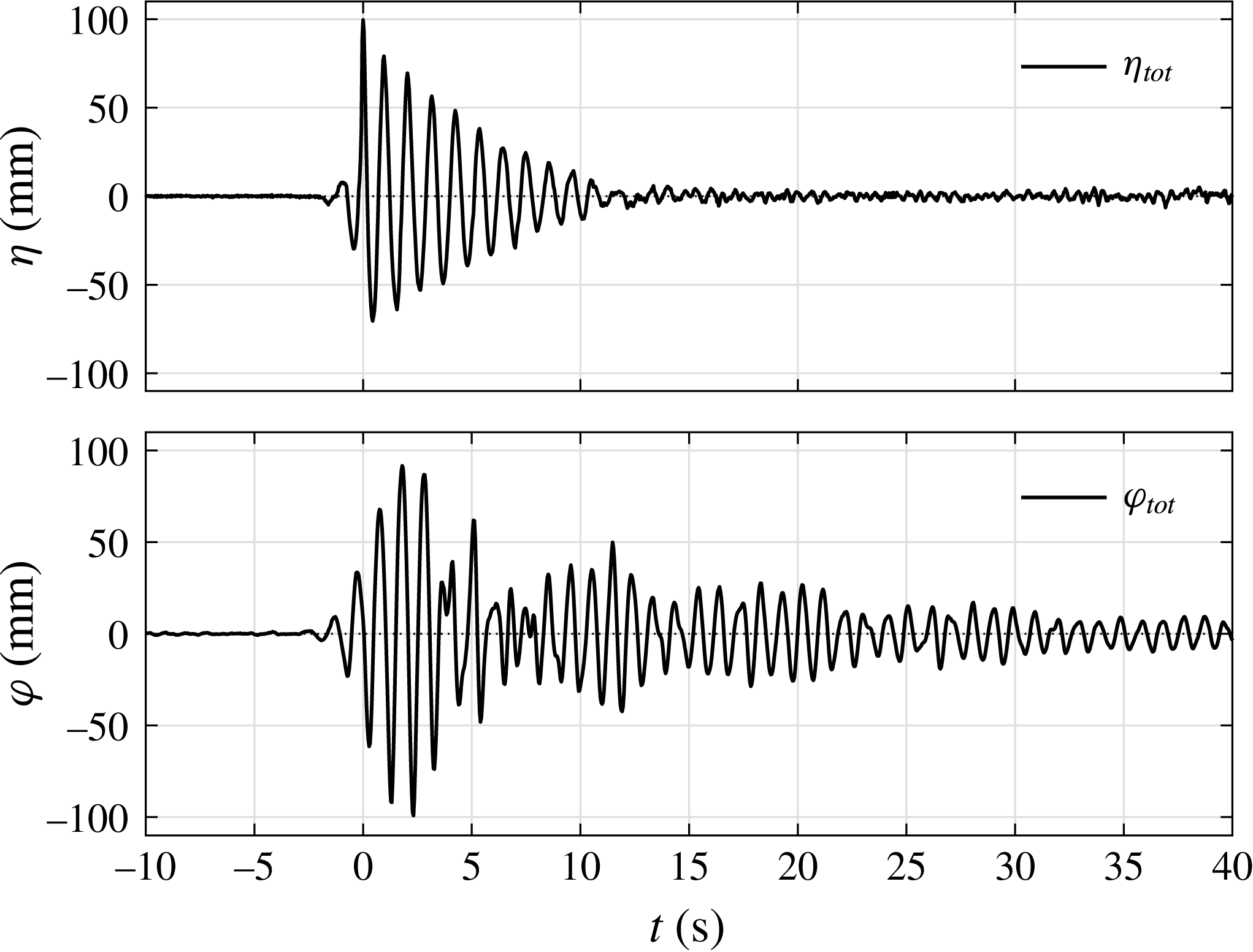
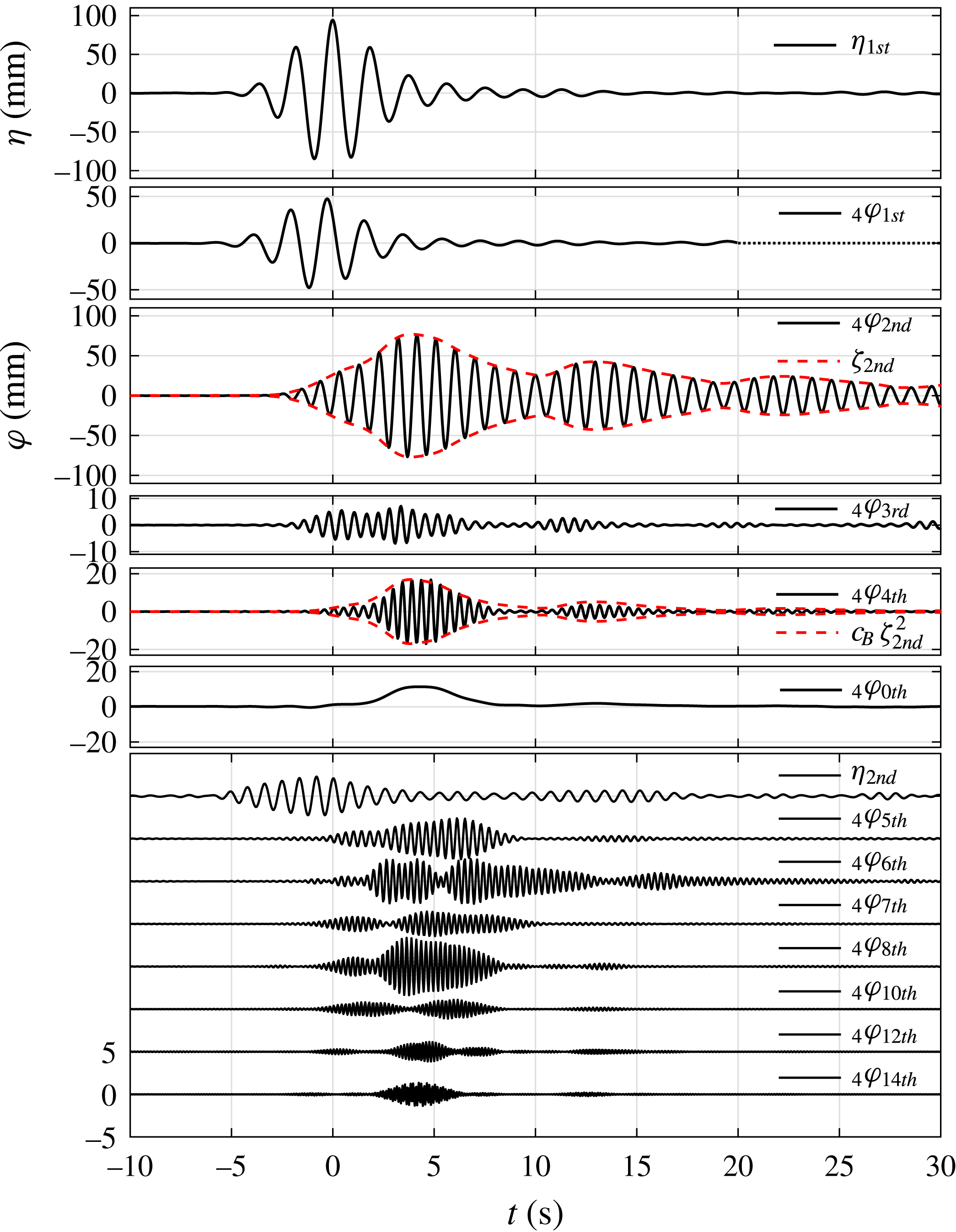
The time histories in figures 23 and 25 show that the gap resonant response is smaller than that of the incident wave group. However, it is interesting to note that the gap resonant response amplitude in figure 25 is a larger fraction of the incident amplitude than for figure 23. This is due to the contribution from the higher harmonics, which will be addressed later. A movie showing the gap motions in set VIB is available in the online supplementary material (movie 4).
As in figure 3, but for set VIB:
 $f_{P}=1/2f_{m=1}$
and
 $\unicode[STIX]{x1D6FC}=100$
mm, beam sea, round bilge, Gaussian spectrum input.


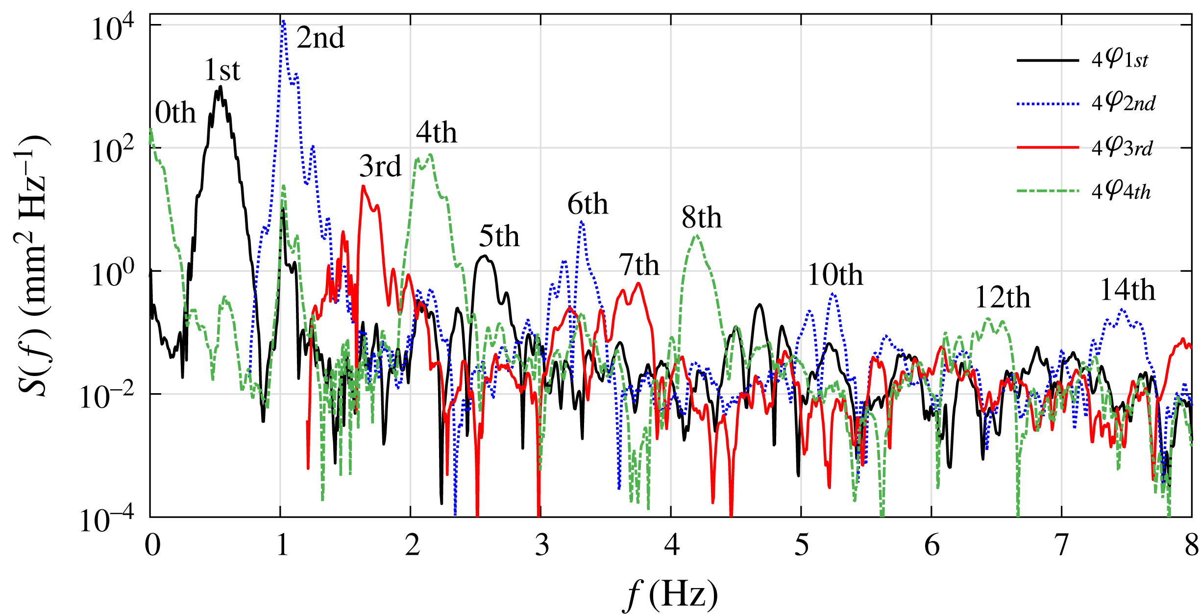
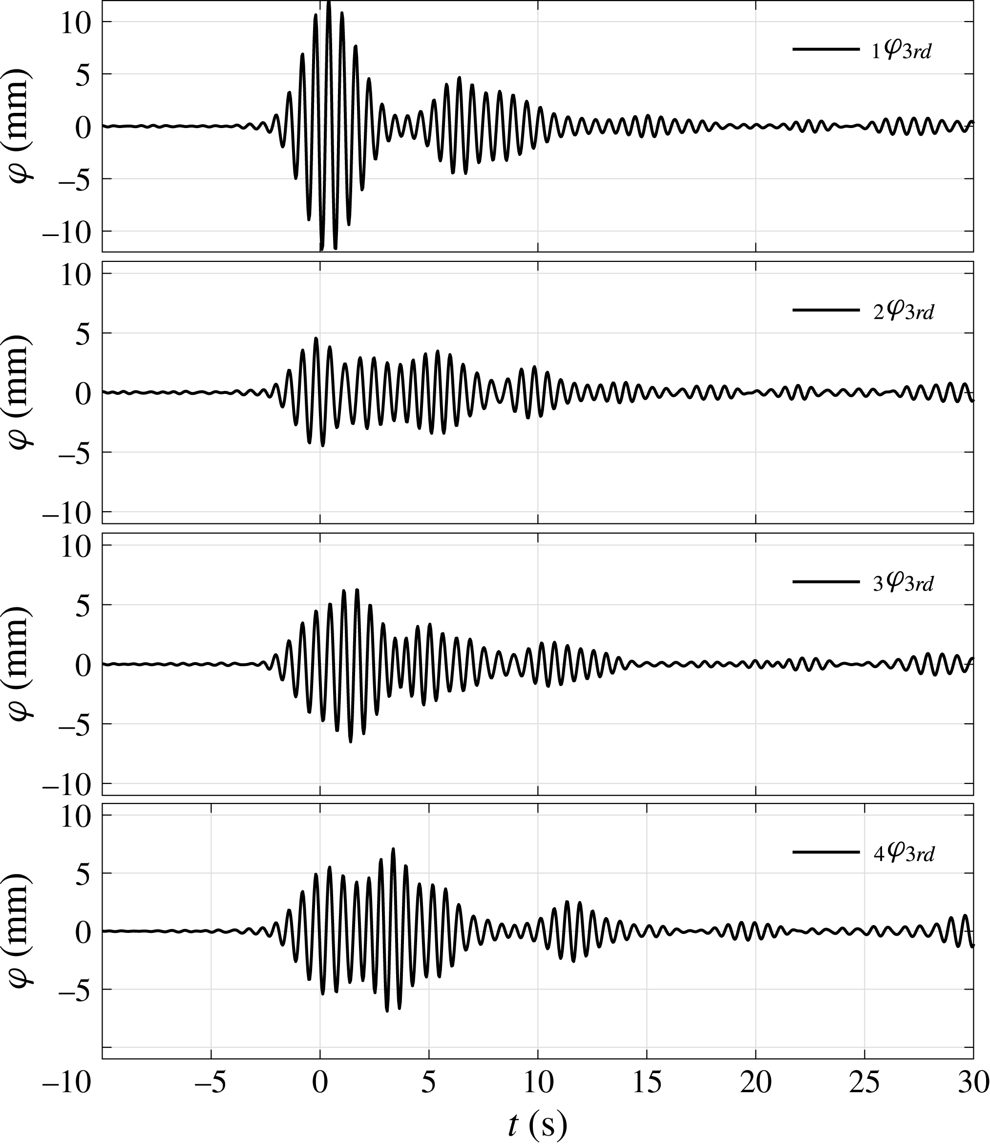
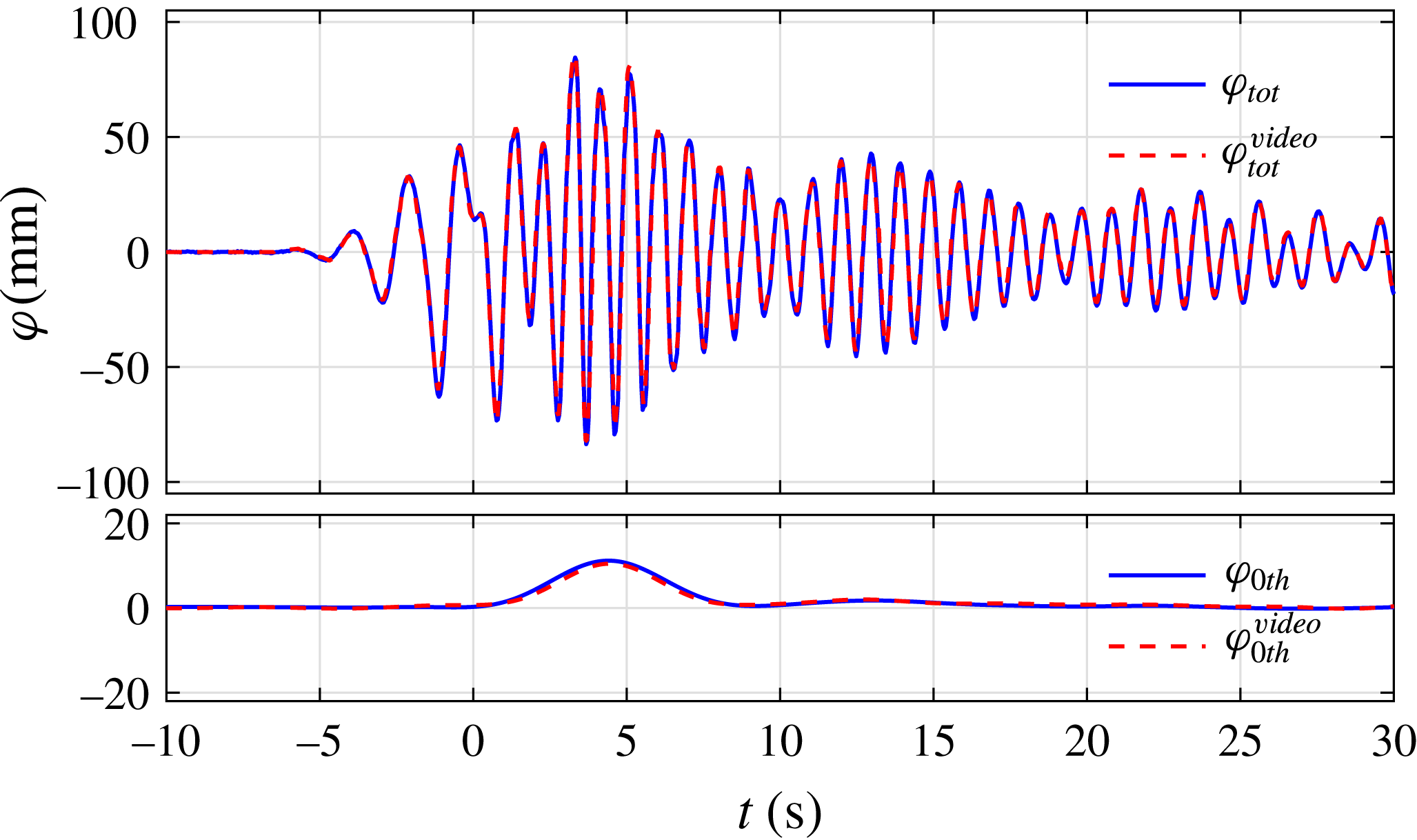
We carried out four-phase combination and digital frequency filtering to obtain the harmonic components (see figure 26). Significant second harmonic components coupling to the gap resonances are observed, which are larger than the first harmonic component. However, the second harmonic component of the incident wave is very small (with a maximum amplitude of 3 mm), contributing only 3 % of the total free-surface elevation (with a maximum amplitude of 100 mm). Therefore, it must be a local quadratic coupling term from the incident half-frequency wave group that drives the gap resonant response as we speculated earlier. As shown in the response spectra (see figure 27), the spectral peak frequencies (2.05, 2.15 and 2.26 Hz) in the fourth harmonic component are the double and cross-frequency terms of the spectral peak frequencies (1.025, 1.125 Hz) in the second harmonic component. Higher harmonic response components have also been excited clearly, even up to the 14th harmonic component, whose maximum surface elevation is approximately 2 mm. To provide more direct evidence, the squared envelope of the second harmonic component is scaled to match the shape of the fourth harmonic component, with good agreement. There is also a significant free-surface set-up in the centre of the gap with an amplitude of 11.4 mm (see the zeroth harmonic in figure 26). As suggested by Molin (Reference Molin2001a ), it is worthwhile to check the WG data independently, particularly for the zeroth harmonic (difference frequency). We compared the WG data with video record data, and found very good agreement (see appendix A). The apparent beating pattern in the higher harmonics is due to the superposition of the different modes of the gap resonant response, which corresponds to the spectral peaks in figure 27. To identify the gap resonant modes driven by the higher harmonic components, we compared the measured data at the four WGs with predicted mode shapes (see figure 28).
Spectra of the harmonics of the gap resonant responses from WG4 for set VIB:
 $f_{P}=1/2f_{m=1}$
and
 $\unicode[STIX]{x1D6FC}=100$
mm, beam sea, round bilge, Gaussian spectrum input. Note that due to our using a four-phase combination method, each signal component contains harmonics separated by four; i.e. the first harmonic signal also contains the fifth, ninth, etc.

Mode shape illustration of the gap resonance driven by second harmonics. The shapes in the vertical direction have been normalised. Set VIB:
 $f_{P}=1/2f_{m=1}$
and
 $\unicode[STIX]{x1D6FC}=100$
mm, beam sea, round bilge, fitted to a Gaussian spectrum.

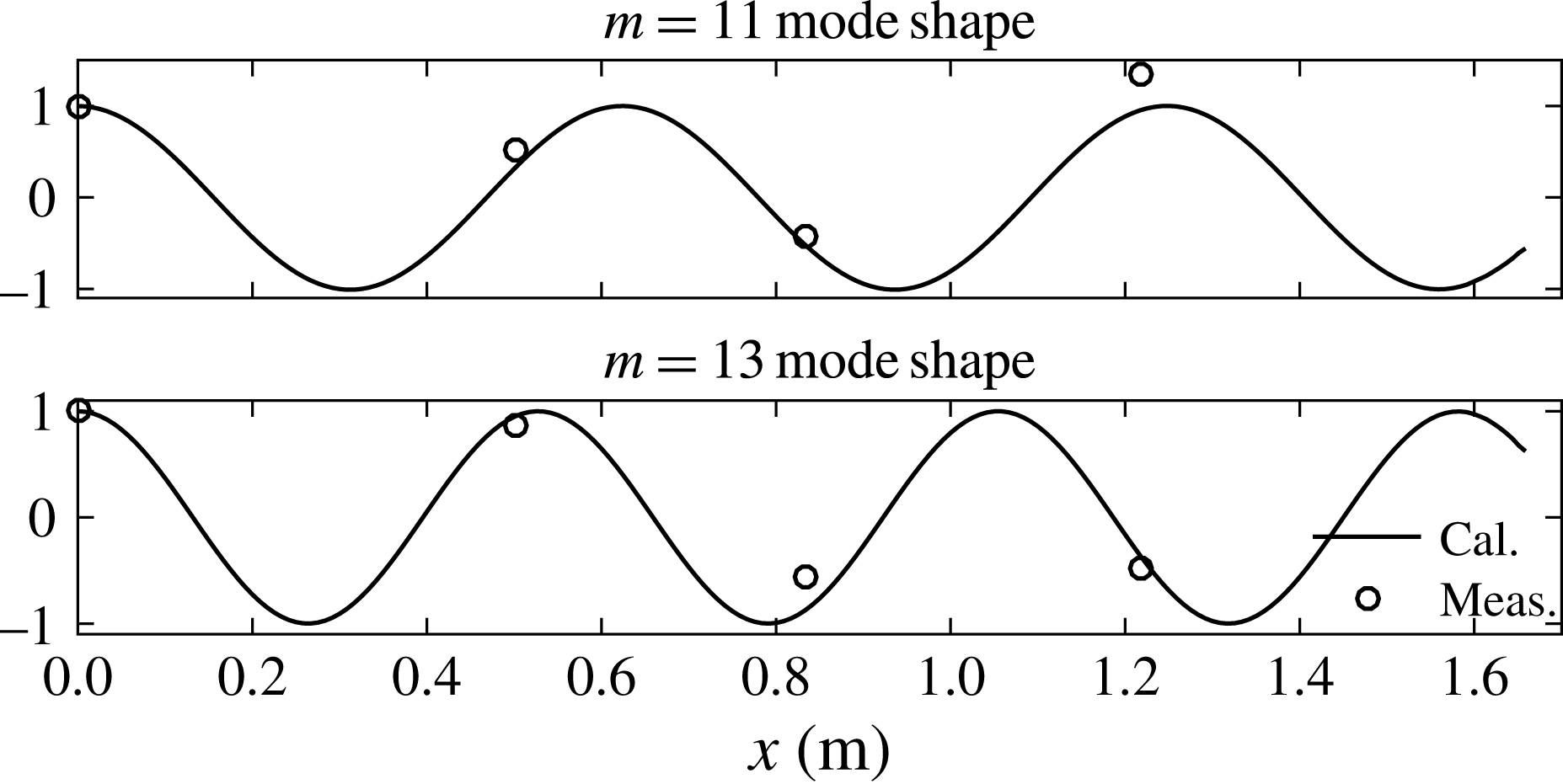
It is difficult to identify the relationship between the other higher harmonics. We take the third harmonic component of the gap resonant response as an example. There can be no double frequency Stokes-type coupling from the second harmonic component with itself, but the third harmonic component persists for much longer than the passage time of the linear component of the input wave. Therefore, this could be associated with higher mode response in the gap. From diffraction calculations, we know that the
 $m=11$
and
 $m=13$
modes have frequencies of 1.62 and 1.75 Hz, which correspond to the frequencies of the highest two spectral peaks of the third harmonic shown in figure 27. This is supported by the results shown in figure 29, which shows the mode shapes extracted from the third harmonic spectra at each WG.
Mode shape illustration of the gap resonance driven by third harmonics (
 $f_{m=11}=1.62$
Hz and
 $f_{m=13}=1.75$
Hz). The shapes in the vertical direction have been normalised. Set VIB:
 $f_{P}=1/2f_{m=1}$
and
 $\unicode[STIX]{x1D6FC}=100$
mm, beam sea, round bilge, fitted to a Gaussian spectrum.

The third harmonic components at different locations for set VIB:
 $f_{P}=1/2f_{m=1}$
and
 $\unicode[STIX]{x1D6FC}=100$
mm, beam sea, round bilge, Gaussian spectrum input.

The third highest spectral peak in the third harmonic (which looks to be below 1.5 Hz) could be the combined contribution of the
 $m=9$
mode gap resonance (
 $f_{m=9}=1.49$
Hz) and a local
 $(\text{linear})^{3}$
source term (
 $0.51\times 3=1.53$
), or/and a second-order interaction between the incident
 $\unicode[STIX]{x1D714}$
wave component and a local
 $2\unicode[STIX]{x1D714}$
standing wave term, producing
 $3\unicode[STIX]{x1D714}$
and
 $\unicode[STIX]{x1D714}$
components. We find in figure 30 (WG4 in the centre of the gap) a second pulse at approximately 12 s, a third one at approximately 20 s and a fourth one at approximately 28 s in the third harmonic response component. This time interval (8 s) could be associated with the frequency difference between the
 $m=11$
and
 $m=13$
modes, i.e. 0.13 Hz.
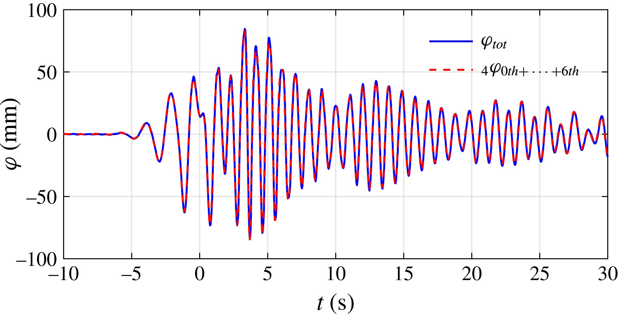
Comparison of the time histories between the original total response signal and the sum of the extracted harmonic components from WG4 for set VIB:
 $f_{P}=1/2f_{m=1}$
and
 $\unicode[STIX]{x1D6FC}=100$
mm, beam sea, round bilge, Gaussian spectrum input.

To check the accuracy of the decomposition of the total signal, we add up the first six (including zeroth) harmonics and compare them with the original total surface elevations in the gap (see figure 31). The very good agreement between the original surface elevations and the sum of the extracted harmonics gives strong evidence that the method is performing well.
Comparison of the time histories from WG4 for sets VIA and VIB. The first harmonic response in set VIA is scaled so as to match that for set VIB, and the same scaling factor and its square are applied to the total signal of the incident group and the second harmonics of the gap response respectively.

It is also interesting to compare the results measured in sets VIA (
 $f_{P}=1/2f_{m=1}$
,
 $\unicode[STIX]{x1D6FC}=50$
mm) and VIB (
 $f_{P}=1/2f_{m=1}$
,
 $\unicode[STIX]{x1D6FC}=100$
mm). To facilitate the comparison, in figure 32 the linear component of the incident NewWave group in set VIA is scaled (with a coefficient of 1.76) to match that in set VIB. The same procedure has been conducted for the linear and second (with a coefficient of
 $1.76^{2}$
) harmonics of the gap resonant responses. The linear components match well for both the incoming wave and the corresponding gap responses. Very slight differences are observed for the second harmonic component of the gap resonant response.
4.8 Damping of the gap resonant modes
As shown previously, the fluid oscillation in the gap decays slowly with a beating pattern after the incident wave has passed. The beating pattern occurs because the different resonant modes present have different frequencies. We investigate the damping of the resonant modes by assuming that the behaviour is linear – thus the decay curves should be well approximated by decaying sinusoids. We therefore conduct a numerical fit to the decay curves using a variant of Prony’s method – the method of Kumaresan & Tufts (Reference Kumaresan and Tufts1982) for estimating damped sinusoids in noise which employs the singular value decomposition (SVD) approach. The Prony-SVD fit assumes a signal of the form
 $$\begin{eqnarray}\unicode[STIX]{x1D711}(t)=\mathop{\sum }_{n}A_{n}\sin (\unicode[STIX]{x1D714}_{n}t+\unicode[STIX]{x1D6FD}_{n})\exp [-\unicode[STIX]{x1D714}_{n}\unicode[STIX]{x1D709}_{n}t],\end{eqnarray}$$
where the subscript
 $n$
represents the number of frequencies
 $\unicode[STIX]{x1D714}_{n}$
that are required for the fit, and the corresponding amplitudes
 $A_{n}$
, phases
 $\unicode[STIX]{x1D6FD}_{n}$
and dimensionless damping coefficients
 $\unicode[STIX]{x1D709}_{n}$
.
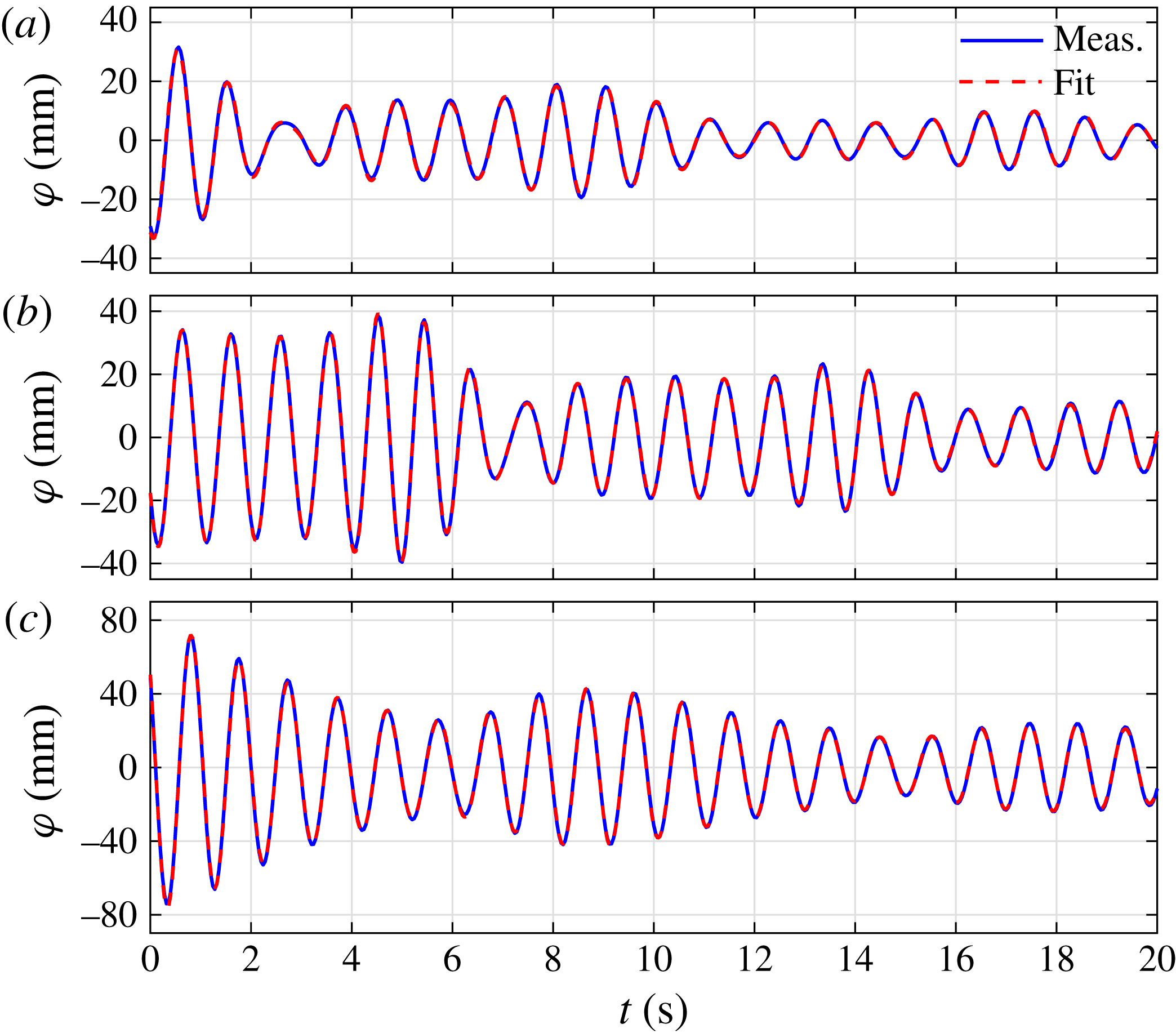
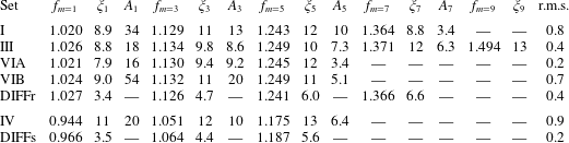
For each test except sets II (head seas) and V, we select a portion of the decay curves from WG1 to WG7 and fit a single set of frequency and damping values to the data. We then use these values to produce an individual amplitude and phase estimate for each of the seven decay curves. For sets I, III and IV, the fit is conducted on the linear signal, and for sets VIA,B the fit is to the second harmonic. We wish to choose a portion of the decay curve that is truly decaying – without excitation from either the incident or reflected waves. The limiting case is set VI, for which reflections return approximately 20 s after the incident wave has passed (see figure 32). Hence, for each test we choose a portion of the decay curves of 20 s in length, commencing when the incident linearised envelope has decreased to 4 % of its peak (sets I, III and IV) or 20 % of its peak (sets VIA,B). Any number of exponentials may be used for the fit, and it is to be expected that adding more will improve the fit. Here, we limit ourselves to physically relevant data by increasing the number of modes until a mode is returned with a frequency that is not present in the spectral data, or is identical to another mode. The results of this procedure are shown in table 4, where the root-mean-square error is calculated over all seven WGs.
Comparison of signals measured at WG4 and reconstructed using a numerical fit to (a) set I, (b) set IV and (c) set VIB. Note that
 $t=0$
is not the focus time in these plots.

Frequencies,
 $f$
(Hz), damping coefficients,
 $\unicode[STIX]{x1D709}\times 10^{3}$
, and amplitudes,
 $A$
, at the start of the window (mm) for each mode of the gap resonant response. The column labelled r.m.s. is the root-mean-square error in mm from all seven WGs. The computed DIFFRACT results for the round and square corner cases are labelled DIFFr and DIFFs respectively.

Also shown in table 4 are the results when an identical procedure is conducted on response time series produced using linear coefficients from our full linear diffraction code DIFFRACT. It is apparent from the table that the numerical fit does a good job of identifying the mode frequencies. Damping values vary slightly from set to set, with more variability in the higher modes, which is to be expected because these signals are a smaller part of the total and harder to fit. It is interesting that the root-mean-square error is smallest for the smallest signal, and largest for the square corner case – if contributions from nonlinear damping were present, this might be expected, although the fit for this case shown in figure 33 is quite good. The root-mean-square error in the square case is affected by the fact that the symmetry of the measured free-surface elevations (
 $\text{WG1}=\text{WG7}$
, etc.) is somewhat worse in this case than the others. No reason for this has been found in the data – the symmetry of WGs just outside the ends of the gap is not so affected.
Comparison with the potential flow results shows clearly that real fluid effects increase the damping, and in particular that the extra damping is substantially larger in the square corner case than the rounded corner case. While the resonant frequencies and measured damping ratios are seen to be closely spaced (increasing by approximately 10 % from one to the next symmetric mode), the damping ratios from the linear potential flow estimates increase rather more substantially. It is observed that each decay rate is a simple exponent in time, and that the rate does not seem to depend on amplitude through the decay, both leading to a linear damping model being appropriate. Hence, a Stokes laminar oscillatory boundary layer is the simplest model possible, where the viscous shear stress, and hence the damping in dimensional form, has an
 $\unicode[STIX]{x1D714}^{1/2}$
dependence (Lamb Reference Lamb1993). Stokes oscillatory laminar boundary layer damping has previously been found to produce reasonable agreement with the experimentally measured linear damping rate for a ring of vertical circular cylinders in resonant ‘near-trapped’ heave motion (Wolgamot et al.
Reference Wolgamot, Taylor, Eatock Taylor, van den Bremer, Raby and Whittaker2016). The dimensions, frequency and amplitude of motion of the cylinder array are all somewhat comparable to those in these gap tests.
(a) Predicted and measured damping ratios (
 $\unicode[STIX]{x1D709}$
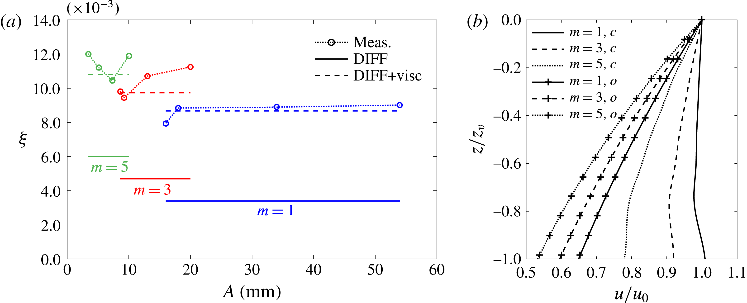
) for the different gap modes versus the amplitude of oscillation. The ‘DIFF’ values, calculated through the linear potential diffraction code DIFFRACT, contain radiation damping only (as in table 4); the ‘visc’ values are generated based on an assumption of Stokes boundary layer damping for the energy dissipation in the gap. (b) Depth variation of the vertical velocity,
 $u$
, for the
 $m=1$
, 3, 5 modes in the gap, at the centre of the gap on the surface of the (downwave) box, denoted by subscript
 $c$
, and in the undisturbed field, denoted by subscript
 $o$
. The variation is calculated using DIFFRACT and is only shown for the flat (vertical) part of the box (with round bilges), down to depth
 $z_{v}=0.102$
m.

If this is the case, the additional damping above radiation damping in the non-dimensional damping ratio,
 $\unicode[STIX]{x1D709}$
, should scale with
 $\unicode[STIX]{x1D714}^{-1/2}$
and be independent of the amplitude of oscillation. This argument should hold for the gap mode oscillations for
 $m=1,3,5,\ldots ,$
as each is distributed with a similar depth variation and sinusoidally with position along the gap. (The depth variation is shown in figure 34(b), and is similar to that given by the analysis of Molin (Reference Molin2001b
), although modified due to the presence of the rounded bilge.) If the difference between the DIFFRACT damping value and averaged total damping value for the
 $m=1$
mode in table 4 is taken as the basis, the extra Stokes term for gap mode
 $m=3$
is this value factored by
 $(f_{m=3}/f_{m=1})^{-1/2}$
(and similarly for
 $m=5$
). This is illustrated in figure 34 (where we did not plot the result for gap mode
 $m=7$
because there are only two data points), and reasonable agreement is observed. If vortex shedding was a major source of damping, we would expect
 $\unicode[STIX]{x1D709}$
to scale with a positive power of frequency and with amplitude, but neither effect is apparent here. Quite different behaviour is apparent for (the more limited data in) the square bilge case. Similar damping analyses by Molin et al. (Reference Molin, Remy, Kimmoun and Stassen2002) for a gap-type structure with square bilges suggested that linear damping was inadequate in this case. It would be possible to estimate the viscous damping for the square bilge case based on a combination of a model for small-amplitude harmonic flows through a slot in a slatted screen (similar to the two-dimensional study by Faltinsen & Timokha (Reference Faltinsen and Timokha2015)) and the wall boundary layer damping model of Molin et al. (Reference Molin, Remy, Kimmoun and Stassen2002), though such an approach has not been tried here.
5 Conclusions
An extensive set of experiments has been carried out with two identical fixed hulls under the excitation of NewWave-type transient wave groups. The purpose has been to investigate the transient characteristics of gap resonant responses, and the first and higher harmonic components of the free-surface elevations in the gap. Unlike regular wave excitation, where the higher harmonics are straightforward to isolate, signal separation is more complicated for wave group excitation due to the terms being driven by products of different spectral components. The four-phase combination method is applied in this study to extract the first four harmonic components, which enables the extraction of individual higher harmonics with simple digital frequency filtering.
Seven WGs were mounted in the gap symmetrically, with WG4 located in the centre. The quality of the experimental set-up has been confirmed through comparison of the wave surface elevations measured by symmetric pairs of WGs mounted in the gap. The time histories of the free-surface elevations in the gap show beating patterns which are the result of excitation of a range of different modes of the gap resonance.
Under a symmetric excitation (in beam seas), which provides symmetric boundary conditions at the ends of the gap, only odd modes of the surface elevations in the gap have been observed. When applying an asymmetric excitation (head seas), both odd and even modes of the surface elevations are excited, with the mode shapes symmetric and antisymmetric with respect to the centre of the gap. The propagation of waves along the gap has been illustrated through the comparison of the time histories of the different harmonic components measured along the gap.
The linear component of the resonant response in the gap is found to be of comparable magnitude to the incident wave groups, so much smaller than that obtained under regular wave excitation. For a focused wave group with a broadbanded spectrum, there is limited time relative to the long duration that is necessary for full development of the gap resonant response. This is well illustrated by the fact that a NewWave derived from a PM spectrum gives a linear response with smaller peaks than a NewWave derived from a Gaussian spectrum, per unit peak amplitude of the incident group, assuming the spectral peak periods of both groups to be the same and chosen to match the first mode resonance of the gap.
To investigate the effect of bilge shape, we also investigated the gap resonant response between vessel hulls with square corners. For this geometry, the resonant frequencies shift downwards a relatively small amount.
In the extremely nonlinear case with wave breaking, we obtained a very spiky shape for the incident NewWave-type group, and the four-phase combination method works less well in extracting higher harmonics. However, the results indicate that higher harmonic response could be significantly driven even by half-frequency input waves.
When excited by an incident wave group with a peak frequency of half the first resonant mode frequency, and maximum surface elevation of
 $\unicode[STIX]{x1D6FC}=50$
mm, we observed more significant higher harmonic components up to fourth order, despite the steepness being substantially less than in the ‘base case’.
Increasing the maximum surface elevation (to
 $\unicode[STIX]{x1D6FC}=100$
mm) of the incident NewWave group excited more higher harmonic components – in this case the first harmonic surface elevation was smaller than the second harmonic, and signals up to 14th order were extracted. The second harmonic component here is driven via quadratic coupling from the incident wave group, and the fourth and zeroth harmonics in the gap are bound to these standing waves.
Offloading of LNG from a floating production vessel (FLNG) into an LNG shuttle carrier will only be attempted in mild sea states. However, almost everywhere in the open ocean, there can be long-period swell from distant storms. In practical applications, this swell would not drive significant surface motion linearly in the gap between the vessels, because it is too low frequency (long period) to couple to the lowest gap mode. However, it is quite possible and has been demonstrated experimentally here that quadratic frequency doubling could occur and couple to the gap resonances. Thus, this interaction should be considered when planning such offshore operations.
A numerical fit to the experimental data has returned linear damping coefficients for each test and for each resonant mode. These clearly show that each mode has a characteristic damping which is independent of the excitation and which is somewhat larger than the damping calculated using linear potential flow theory alone. The additional viscous damping appears to be slightly different for each mode. The data provide some support to the suggestion that for the round bilge cases, viscous damping at the scale tested is dominated by linear boundary-layer-type effects. Different behaviour is observed for square bilges.
Acknowledgements
This work was funded by research and development grants from the University of Western Australia (UWA) and from Shanghai Jiao Tong University (SJTU). The first two authors are grateful for support through the Shell EMI Offshore Engineering Initiative at UWA. The authors acknowledge the discussion with Professor J. Yang at SJTU and Professor M. Efthymiou and Dr S. Draper at UWA.
Supplementary movies
Supplementary movies are available at https://doi.org/10.1017/jfm.2016.824.
Appendix
Free-surface elevations measured using WGs are crucial to this study. Here, we briefly present some checks that were made on the data quality. The WGs were calibrated prior to the model tests. The maximum surface elevation in this study is approximately 100 mm, so we chose
 $\pm 150$
mm as the calibration range. Figure 35 shows representative calibration data, indicating linear response within this range.
A representative calibration result of the WGs;
 $\unicode[STIX]{x1D702}$
is the surface elevation and
 $U$
is the voltage signal.

Comparison of the data measured by the WG and estimated from the video record at the centre of the gap (WG4) for set VIB.

To provide further evidence of the high quality of the measured data, WG measurements were compared with measurements derived from video footage. In the model tests, a video camera was fixed in one of the boxes so as to record the water surface elevations in the centre of the gap through a transparent window. As shown in the online supplementary material (movie 2), there is a chessboard grid with 1 cm squares fixed on the outside of the other box to provide a visual reference. We have therefore estimated the surface elevations in a large number of frames to produce time series – for set VIB we show (in figure 36) a comparison between the measurements thus derived and the WG data. In figure 36, we also display a comparison for the zeroth harmonic, produced from the video data by low-pass filtering. The WG data agree very well with the camera data both in the total signal and in the zeroth harmonic.