




1. Introduction
There are several regimes of interest in turbulent combustion. One that is very frequently encountered is the flamelet regime, where chemistry is relatively fast and reactions take place in thin layers. Many technical applications fall into this regime; therefore, prediction methods based on the flamelet concept are often used to model combustion in engines and gas turbines. In this framework, a turbulent flame is viewed as an ensemble of thin flamelet structures. The flamelet structure is laminar in nature and attached to an instantaneous flame surface, which is corrugated by turbulence. The concept applies to premixed as well as non-premixed combustion. In the case of non-premixed combustion, the assumption of infinitely fast reactions leads to the flame sheet model having an infinitely thin flame structure. As the turbulent mixing is the sole rate-determining process in this regime, the description of non-premixed combustion can be fully described by the transport of the mixture fraction
 \begin{equation} Z = \frac{m_1}{m_1+ m_2} \end{equation}
with  $m_1$ and
 $m_2$ denoting the local mass originating of the fuel and the oxidizer, respectively.
The departure from this limit requires the consideration of finite rate chemistry and can be described by the laminar diffusion flamelet concept (Peters Reference Peters1984). Flamelet equations can be derived by transforming the transport equations for temperature and species mass fractions into equations with the mixture fraction  $Z$ as the independent variable, yielding equations for the species fractions and temperature as
 \begin{gather} \rho\frac{\partial Y_\alpha}{\partial t} - \rho\frac{\chi}{2}\frac{\partial^2 Y_\alpha}{\partial Z^2} =\omega_\alpha, \quad \alpha = 1,2,\dots,k , \end{gather}
 \begin{gather}\rho\frac{\partial T}{\partial t} - \rho \frac{\chi}{2}\frac{\partial^2 T}{\partial Z^2} = \omega_{T} , \end{gather}
where  $\chi$ is the scalar dissipation rate
 \begin{equation} \chi = 2D\left(\frac{\partial Z}{\partial x_i} \right)^2 . \end{equation}
In the equation for the chemical species,  $\rho$ is the density,
 $Y_\alpha$ is the mass fraction of species
 $\alpha$,
 $t$ is the time,
 $Z$ is the mixture fraction and
 $\omega _\alpha$ is the chemical source term for species
 $\alpha$. In the temperature equation,
 $T$ is the temperature,
 $\omega _T$ is the heat release term due to chemical reactions and
 $D$ is the diffusion coefficient of the mixture fraction. Since transport in the outer, chemically inert structure of the flame is mostly governed by turbulence, which leads to similar transport for all scalars (Attili et al. Reference Attili, Bisetti, Mueller and Pitsch2016), all Lewis numbers are assumed be unity
 $\mathit {Le}_\alpha =\lambda /(c_{{p}} \rho D_\alpha ) = 1$, with the thermal conductivity
 $\lambda$, the heat capacity
 $c_{p}$ and the diffusion coefficient of the species
 $D_\alpha$. Additional terms containing spatial derivatives orthogonal to
 $Z$, can be neglected to the leading order. The scalar dissipation rate
 $\chi$ serves as the quantity which connects the reacting scalar field to the turbulent flow field.
For intense turbulence, when turbulent scales are small compared to the scales of the flame, the implied separation of turbulent and chemical scales in the laminar diffusion flamelet concept is expected to fail (Bilger et al. Reference Bilger, Pope, Bray and Driscoll2005; Pope Reference Pope2013). The flame structure and the rate of mixing then start to be affected by interactions between reaction, diffusion and turbulent straining. Another shortcoming is that even in the case of thin structures for the combustion reactions not all reactions are sufficiently fast. This is the case for the chemical processes governing pollutants like  $\mathrm {NO}_x$ and soot, because their chemistry may be comparably slow. Furthermore, close to extinction or during ignition, when combustion becomes slow or when chemistry competes with diffusive losses in more than one direction, which is known as the edge flame effect (Favier & Vervisch Reference Favier and Vervisch2001), the flamelet assumption of a thin one-dimensional layer will cease to be valid.
To identify and analyse spatial regions of the turbulent reacting flow, which either correspond to flamelet-‘friendly’ conditions or are dominated by small-scale turbulence and extinction-inducing turbulence intensities, a systematic method for compartmentalization of the turbulent fields is required. A method for a physically motivated decomposition of turbulent scalar fields is the dissipation element (DE) analysis. This analysis considers space-filling spatial regions of a scalar field and has been proposed by Wang & Peters (Reference Wang and Peters2006, Reference Wang and Peters2008). DEs are constructed by using gradient trajectories. Starting from every point in the field, a scalar gradient trajectory in the ascending direction will reach a maximum point, and in the descending direction, it will reach a minimum point. A DE is defined as the spatial region from which the same pair of maximum and minimum points is reached by scalar gradient trajectories. Within this region, the scalar field is monotonic making DEs equivalent to Morse–Smale complexes in topology (Schnorr et al. Reference Schnorr, Helmrich, Denker, Kuhlen and Hentschel2020). This method of identification of DEs is shown in a schematic fashion in figure 1.
Exemplary decomposition of a two-dimensional scalar field by means of a DE analysis. Iso-scalar lines are shown in black. The black symbols show two sample points with associated gradient trajectories towards the scalar maximum (red) and minimum (blue).

DEs are characterized by two parameters, henceforth called DE parameters: the length  $\ell$ is defined as the linear distance between the minimum and maximum points and
 ${\rm \Delta} \phi$ is the difference of the scalar value at these two points. In addition to these two DE parameters, a measure for the scalar gradient can be formed as
 $g = {\rm \Delta} \phi / \ell$.
In Wang & Peters (Reference Wang and Peters2006, Reference Wang and Peters2008), Gampert et al. (Reference Gampert, Schaefer, Goebbert, Wang and Peters2010), Gampert et al. (Reference Gampert, Goebbert, Schaefer, Gauding, Peters, Aldudak and Oberlack2011), Peters (Reference Peters2012), Gampert et al. (Reference Gampert, Schaefer, Goebbert and Peters2013a) and Gampert, Schaefer & Peters (Reference Gampert, Schaefer and Peters2013b), three-dimensional (3-D) direct numerical simulations (DNS) of non-reactive flows were performed in order to obtain the statistics of the DE parameters in turbulent flows. The joint probability density function (jPDF)  $P(\ell , {\rm \Delta} \phi )$ of the two DE parameters
 ${\rm \Delta} \phi$ and
 $\ell$ is expected to be sufficient to statistically reconstruct most of the scalar field. Several physical effects can be identified in this jPDF, such as the presence of ramp-cliff structures, annihilation of DEs due to molecular diffusion and high spatial gradients caused by intermittency. In these studies, the DE analysis provided a valuable tool for describing and investigating the effect of turbulent and diffusive transport on scalar fields.
Applying DE analysis to reacting turbulent flows provides multiple additional modes of assessment and a new interpretation of DEs in this physical context. It allows the investigation of non-local effects and interactions in complex combustion conditions by providing a well-parametrized and physically meaningful frame of reference. Further, by investigating the interaction between turbulence and combustion chemistry locally within individual DEs, flow dynamics and topology can be considered, while they would otherwise be lost in the averaging procedure used in conventional statistical approaches.
The DE analysis was first applied to the DNS of a non-premixed flame by Gauding et al. (Reference Gauding, Dietzsch, Goebbert, Thévenin, Abdelsamie and Hasse2017), where DEs were used to compartmentalize regions of the scalar field which are either connected by diffusive flux to the flame front, the turbulent core region or the outer regions of the flow. Additionally, DE analysis was applied to temperature fields by Denker et al. (Reference Denker, Attili, Luca, Gauding, Bisetti and Pitsch2019) to investigate the effects of the premixed flame front on turbulent scalar fields in a series of premixed jet flames (Luca et al. Reference Luca, Attili, Lo Schiavo, Creta and Bisetti2019). The source term present in the temperature fields resulted in a distinct departure from the characteristic features of the DE parameters observed in non-reacting flows.
The DE analysis is applied here to the series of reacting DNS of non-premixed combustion outlined in the next section. In addition, selected non-reactive cases are also considered for comparison. In particular, statistics of the DE parameters are compared among the reacting and non-reacting cases to evaluate the effect of heat release on the scalar fields. The correlation of DE parameters and reacting scalars is investigated to demonstrate the importance of considering non-local effects in the investigated combustion conditions. A comparison of the flame scales with the local turbulent scales provided by the DEs is used to define a new regime diagram for turbulent non-premixed combustion based on the DE parameters. Contrary to conventional approaches to regime classifications, which employ global statistical quantities, the regimes are based on the instantaneous scalar topology and therefore allow for the coexistence and assessment of multiple regimes in a single flame. Finally, the regime diagram is used in a local classification of the combustion of the individual cases.
2. Configurations and numerical methods
2.1. DNS configuration of the reactive and non-reactive jets
The configuration selected for this study is a temporally evolving planar jet. This configuration lends itself to the DNS as it provides a good ratio between grid points and the overall volume of reacting flow. Besides displaying self-similarity in non-reacting configurations, the two statistically homogeneous directions simplify the computation of well-converged statistics.
Three different jet Reynolds numbers  $\mathit {Re}_{{jet}} = \bar U_0 H_0 / \nu _{{fuel}}$, with initial mean jet bulk velocity
 $\bar U_0$, initial jet width
 $H_0$ and kinematic viscosity
 $\nu _{{fuel}}$ of the fuel, were realized. The values of the Reynolds numbers range from 4500 to 10 000.
Multiple Reynolds numbers are required to investigate the distinctive scaling of DE parameters, which was observed in non-reacting flows by Wang & Peters (Reference Wang and Peters2006, Reference Wang and Peters2008, Reference Wang and Peters2013). In addition to the change in Reynolds numbers, two different dilutions of the fuel stream were used for the lowest Reynolds number. These four cases will be referred to as the low  $\mathit {Re}$ low dilution case, the low
 $\mathit {Re}$ high dilution case, the intermediate
 $\mathit {Re}$ case and the high
 $\mathit {Re}$ case. The turbulent Damköhler number
 $\mathit {Da} = \chi _{q} H / U_{c,0}$ is set to
 $\mathit {Da} = 0.125$ for the low
 $\mathit {Re}$ low dilution case and the low
 $\mathit {Re}$ high dilution case and to
 $\mathit {Da} = 0.15$ for the other two high dilution cases. These values were chosen to induce local extinction and provide the basis for the investigation of extinction processes. At the final time step of the simulation, this resulted in approximately
 $5\,\%$,
 $11 \,\%$,
 $16 \,\%$ and
 $24\,\%$ of extinguished flame surface for the
 $\mathit {Re}$ low dilution case, for the
 $\mathit {Re}$ high dilution case, for the intermediate
 $\mathit {Re}$ case, and high
 $\mathit {Re}$ case, respectively.
The oxidizer stream in all reacting cases is air, consisting of oxygen  $Y_{\mathrm {O}_{2},1} = 0.232$ and nitrogen
 $Y_{\mathrm {N}_{2},1} = 0.768$. The fuel stream consists of highly diluted methane with
 $Y_{\mathrm {CH}_{4},2} = 0.232$ for the low dilution case and
 $Y_{\mathrm {CH}_{4},2} = 0.07$ for the high dilution cases. The indices
 $1$ and
 $2$ indicate the oxidizer and the fuel properties, respectively. The dilution of the fuel stream is achieved with
 $\mathrm {N}_{2}$. This results in a stoichiometric mixture fraction of
 $Z_{{st}} = 0.2$ for the low
 $\mathit {Re}$ low dilution case and
 $Z_{{st}} = 0.45$ for the low
 $\mathit {Re}$ high dilution case, the intermediate
 $\mathit {Re}$ case and the high
 $\mathit {Re}$ case. These high dilutions were chosen for two reasons: First, to provide sufficient distance between the turbulent/non-turbulent interface (TNTI) and the flame surface. Second, to provide a wide reaction zone thickness in mixture fraction space
 $\delta Z_{r}$. The temperature for both oxidizer and fuel was set to
 $T_1 = T_2 = 500\ \textrm {K}$ for the low dilution case. To increase the resistance to the turbulence-induced strain, the temperature for the high dilution cases was raised to
 $T_1 = T_2 = 680\ \textrm {K}$. The quenching dissipation rate for all cases is
 $\chi _{q} = 120\ \textrm {s}^{-1}$.
The flow configuration of the reacting cases is shown schematically in figure 2. The domains are periodic in the streamwise  $x$-direction and spanwise
 $z$-direction. Boundary conditions in the cross-wise
 $y$-direction were chosen as outlets (Ol'shanskii & Staroverov Reference Ol'shanskii and Staroverov2000).
General set-up of the DNS investigated in this study. The grey iso-surface indicates the position of the stoichiometric mixture fraction.

This resolution was chosen to ensure a sufficiently resolved reaction zone with a minimum thickness of the  ${\textrm {OH}}$-layer of
 $10$ grid points at all times. This resolution was used in a number of DNS studies of non-premixed combustion for similar configurations (Hawkes et al. Reference Hawkes, Sankaran, Sutherland and Chen2007; Attili et al. Reference Attili, Bisetti, Mueller and Pitsch2014), where the quality of the results and the resolution requirements where assessed in detail. The minimum Kolmogorov scale is
 $\eta = 209\ \mathrm {\mu }\textrm {m}$, with
 $\eta = \nu ^{3/4} \varepsilon ^{-1/4}$, for the low
 $\mathit {Re}$ low dilution case,
 $\eta =281\ \mathrm {\mu }\textrm {m}$ for the low
 $\mathit {Re}$ high dilution case,
 $\eta =245\ \mathrm {\mu }\textrm {m}$ for the intermediate
 $\mathit {Re}$ case and
 $\eta =233\ \mathrm {\mu }\textrm {m}$ for the high
 $\mathit {Re}$ case. From this follows that
 $\varDelta / \eta \approx 0.76$,
 $\varDelta / \eta \approx 0.74$,
 $\varDelta / \eta \approx 0.85$ and
 $\varDelta / \eta \approx 0.86$, respectively. This high resolution is required for a meaningful result of a DE analysis (Wang & Peters Reference Wang and Peters2006). Additional details regarding the numerical and physical parameters of the DNS are summarized in table 1.
Numerical and physical initial parameters of the DNS. Where needed, the parameters for the non-reacting case II were re-computed with the given values for  $\bar {U}_{0}$ and
 $H_0$.

The velocity field in the jet core was initialized with instantaneous realizations of turbulent channel flows. The mixture fraction field was initialized by integrating  $\chi (Z) = a \exp (-2 [ \text {erfc}^{-1}(2 Z)]^2) = 2 D(Z)(\partial Z / \partial y)^2$ in the
 $y$-direction from
 $Z = 0$ (oxidizer) to
 $Z = 1$ (fuel). The mixture fraction profile starts at the edge of the channel velocity profile at
 $y = \pm 0.5 H_0$ to provide a wider fuel slab to maintain combustion during later time steps and allow the velocity field to develop. The parameter
 $a$ was chosen so that the dissipation rate at stoichiometric conditions
 $\chi _{{st}}$ is set to
 $\chi _{{st}} = 40\ \textrm {s}^{-1}$ for the low dilution case and
 $\chi _{{st}} = 10\ \textrm {s}^{-1}$ for the high dilution cases. This difference in the initial scalar dissipation rate is chosen because of the significantly closer proximity of the position of the initial stoichiometric mixture to the velocity profile for the high dilution cases. The temperature and species mass fractions are mapped onto the mixture fraction field from a steady state flamelet solution with a non-unity Lewis number obtained in a counterflow configuration following Pitsch & Peters (Reference Pitsch and Peters1998).
The initial profiles of the streamwise velocity component and the mixture fraction are shown in figure 3. The normalized initial velocity profiles of the reacting cases differ slightly due to the different Reynolds numbers of the turbulent channel flows used in the initialization.
Starting profiles of the streamwise mean velocity component  $\bar {U}_0$ (solid lines) and starting profiles of the mixture fraction
 $\bar {Z}_0$ and passive scalar
 $\phi _0$ (dashed lines).

In addition to the three reacting cases, a DNS of a non-reacting planar temporally evolving jet was conducted. This DNS will be referred to as non-reacting case I. The numerical set-up, domain dimensions and initial Reynolds number mirror the intermediate  $\mathit {Re}$ case. The initial velocity field is initialized using the same instantaneous velocity field of a turbulent channel flow employed in the initialization of the intermediate
 $\mathit {Re}$ case. Material properties of the flow are homogeneous and obtained from the fuel composition of the reacting cases of
 $Y_{\mathrm {CH}_{4},2} = 0.07$ and
 $Y_{\mathrm {N}_{2},2} = 0.93$ at
 $T = 680\ \textrm {K}$. A passive scalar
 $\phi$ was added, ranging from
 $0$ to
 $1$. The initial
 $\phi$ is that of the mixture fraction profile of the reactive case of the same Reynolds number. The Schmidt number of the passive scalar was set to
 $\mathit {Sc}_{\phi } = 0.77$. The ratio of the minimum Kolmogorov scale to the grid resolution is
 $\varDelta / \eta \approx 1.1$. Finally, a non-dimensional, non-reacting DNS, from this point on referred to as non-reacting case II, will serve as another dataset to include a more widely used jet configuration with traditional initial solution at a higher Reynolds number (Stanley, Sarkar & Mellardo Reference Stanley, Sarkar and Mellardo2002; Taveira & da Silva Reference Taveira and da Silva2013; Hunger, Gauding & Hasse Reference Hunger, Gauding and Hasse2016). This configuration possesses periodic boundary conditions in both the streamwise
 $x$ and the spanwise
 $z$ directions and free-slip conditions in the cross-stream direction
 $y$. The non-dimensional size of the domain is
 $L_x \times L_y \times L_z = 6 {\rm \pi}\times 12.5 \times 6{\rm \pi}$. Non-dimensionalization of the transport equations is performed with the initial velocity
 $\bar U_{0}$, the initial jet thickness
 $H_0$ and the maximum initial scalar value
 $\phi _{{max}, 0}$. The streamwisevelocity component and the passive scalar field are prescribed via a hyperbolic tangent profile. In the core region, the initial velocity is perturbed with a broadband random Gaussian velocity field derived from a one-dimensional turbulent energy spectrum to speed up the laminar–turbulent transition. The initial jet Reynolds number is set to
 $\mathit {Re}_{{jet}} = \bar U_{0}H_0 /\nu = 9850$. The resolution in the core region is
 $\varDelta / \eta \approx 1.4$.
2.2. Numerical methods
The DNS of the reactive flows were performed with the reactive, unsteady Navier–Stokes equations in the low Mach number limit using the in-house Solver CIAO (Desjardins et al. Reference Desjardins, Blanquart, Balarac and Pitsch2008). The transport of species mass fractions is described using the Hirschfelder and Curtiss approximation to the diffusive fluxes together with a velocity-correction approach for mass conservation (Attili et al. Reference Attili, Bisetti, Mueller and Pitsch2016). Momentum equations are spatially discretized with a fourth-order scheme.
The disturbance pressure is obtained by solving the Poisson equation using the multi-grid solver HYPRE-AMG (Falgout, Jones & Yang Reference Falgout, Jones and Yang2005). Species and temperature equations are discretized with a fifth-order weighted essentially non-oscillatory (WENO) scheme (Jiang & Shu Reference Jiang and Shu1996). The temperature and species equations are advanced by introducing the symmetric operator split of Strang (Reference Strang1968). The two independent operators account for transport and reaction. The chemistry operator uses a time-implicit backward difference method (Hindmarsh et al. Reference Hindmarsh, Brown, Grant, Lee, Serban, Shumaker and Woodward2005). For further details about the applied numerical algorithms and code verification, the reader is referred to Desjardins et al. (Reference Desjardins, Blanquart, Balarac and Pitsch2008). Combustion is modelled using a reduced mechanism for the oxidation of methane comprising  $28$ species and
 $102$ reactions (Peters et al. Reference Peters, Paczko, Seiser and Seshadri2002). Additionally, the formation of
 $\mathrm {NO}$ is included by means of the Zeldovich mechanism (Lavoie, Heywood & Keck Reference Lavoie, Heywood and Keck1970).
The DNS of the non-reactive flow is performed by solving the non-dimensional unsteady incompressible Navier–Stokes equations employing the in-house Solver psDNS (Göbbert et al. Reference Göbbert, Iliev, Ansorge, Pitsch, Di Napoli, Hermanns, Iliev, Lintermann and Peyser2017). Additionally, an advection–diffusion equation is solved for a passive scalar. Spatial derivatives are calculated by the implicit sixth-order finite difference compact scheme introduced by Lele (Reference Lele1992). The temporal integration is performed by employing a low storage fourth-order Runge–Kutta method. The Poisson equation is solved in spectral space by adapting a Helmholtz equation (Cook, Cabot & Miller Reference Cook, Cabot and Miller2004).
3. Turbulent flame analysis
The overall flame evolution is shown for two different normalized time instants  $t^*= 10$ and
 $t^* = 20$ in figure 4. The non-dimensional time
 $t^*$ is defined as
 $t^* =(t-{\rm \Delta} t_{\widetilde {\chi _{{st}}''^2} = 0})/ t_{{j}}$. The jet time is defined as
 $t_{{j}} = H_0/\bar U_0$. In addition, the duration for which the variance of the scalar dissipation rate at stoichiometric conditions is zero
 ${\rm \Delta} t_{\widetilde {\chi _{{st}}''^2} = 0}$ is introduced. The subtraction with
 ${\rm \Delta} t_{\widetilde {\chi _{{st}}''^2} = 0}$ accounts for the varying time among the cases before the turbulent central flow reaches the surface of the stoichiometric mixture fraction due to the different initial fuel slab sizes. The two time steps correspond to the time of the maximum variance of the scalar dissipation rate at stoichiometric conditions,
 $t^*= 10$, and the final time step in the simulations,
 $t^*= 20$.
Mixture fraction  $Z$ in the
 $x$–
 $y$ centre plane at time steps
 $t ^*= 10$ (a,c,e,g) and
 $t^* = 20$ (b,d,f,h). From top to bottom: low
 $\mathit {Re}$ low dilution case, low
 $\mathit {Re}$ high dilution case, intermediate
 $\mathit {Re}$ case and high
 $\mathit {Re}$ case. The red colour indicates the fuel stream, blue the oxidizer. The iso-contour of the stoichiometric mixture fraction is indicated by a red line. The presence of
 $\mathrm {OH}$ is indicated by the iso-contour of
 $Y_{\mathrm {OH}} = 0.01 Y_{\mathrm {OH},{flamelet}}( Z_{{st}})$ by the white lines. The regions of quenching dissipation rates
 $\chi \geq \chi _{{q}}$ are indicated by black contours.

The mixture fraction  $Z$ is shown in figure 4. The increase in wrinkling and folding of the flames due to turbulent advection, while present in the low dilution case, is more pronounced in the high dilution cases. High dissipation rates of the mixture fraction variance can lead to local extinction and such extinguished regions can re-ignite once the scalar dissipation rate has decreased. Although extinction and especially re-ignition do not occur instantaneously (Sripakagorn et al. Reference Sripakagorn, Mitarai, Kosaly and Pitsch2004), the magnitude of the dissipation rate still provides an indication of the expected dynamics in a certain region. Regions where the scalar dissipation rate exceeds the quenching dissipation rate of the stationary flamelet solution
 $\chi \geq \chi _{{q}}$ are encompassed by a black contour. The regions of high
 $\chi$ are predominantly present in the rich regions of flow close to
 $Z_{{st}}$. To indicate the burning flame regions and extinguished regions of the flame, a threshold of the
 $\mathrm {OH}$ mass fraction obtained from the steady state flamelet solution
 $Y_{\mathrm {OH}} (x_i) = 0.01 Y_{\mathrm {OH}}( Z_{{st}}, \chi _{q})$ is plotted as a white iso-line. As the simulations were initialized with two fully burning flames, all regions surrounding the stoichiometric mixture fraction were initially burning and consequently also contained high concentrations of
 $\mathrm {OH}$. Therefore, at the time shown in figure 4, any stoichiometric regions with very low values of
 $Y_{\mathrm {OH}}$ are considered extinguished here and must have experienced high dissipation rates in their history. If these regions have low values of the dissipation rate at the time shown in figure 4, they might be in the process of re-igniting, which, however, is often a slow process (Sripakagorn et al. Reference Sripakagorn, Mitarai, Kosaly and Pitsch2004). While all the cases display mostly intact flames, the later times show more extinguished regions in the process of re-ignition due to the aforementioned effect.
The temporal evolution of the normalized mean  $\widetilde {\chi _{{st}}}$ at stoichiometric conditions is shown in figure 5(a). Qualitatively, the temporal evolutions display the same features for all cases. The shape of the temporal evolution of
 $\widetilde {\chi _{{st}}}$ is characteristic of the configuration of the planar temporally evolving jet and is observed also in other reacting and non-reacting jets (Attili et al. Reference Attili, Bisetti, Mueller and Pitsch2016; Hunger et al. Reference Hunger, Gauding and Hasse2016). The steep increase of
 $\widetilde {\chi _{{st}}}$ is a result of increasing gradients caused by the formation of turbulence. The scalar dissipation rate experiences a peak and then enters an equilibrium state with the other turbulent fields, indicated by the exponential decay. Here, gradients decrease again as a result of the increasing length scales of the system.
(a) Temporal evolution of the normalized Favre averaged scalar dissipation rate conditioned on the stoichiometric mixture fraction. (b) Temporal evolution of the normalized area of the iso-surface of the stoichiometric mixture fraction (solid) and burning area (dashed). Normalization is achieved with the initial stoichiometric iso-surface  $A_{{st,0}} = 2 L_x L_z$. Burning regions of the stoichiometric iso-surface are identified by thresholding the local OH mass fraction
 $Y_{\mathrm {OH},{burning}} = Y_{\mathrm {OH}}(Z = Z_{{st}}) \geq 0.1 Y_{\mathrm {OH},{flamelet}}( Z_{{st}}, \chi _{q})$.

The temporal development of the total surface area of the stoichiometric iso-surface  $A_{{st}}$ is shown in figure 5(b).
 $A_{{st}}$ is normalized with the initial stoichimetric iso-surface area
 $A_{{st,0}} = 2L_xL_z$. The significantly bigger difference in stoichiometric iso-surface growth between the low dilution case and high dilution cases is indicative of a higher influence of the stoichiometry than the Reynolds number in these simulations. The low Damköhler number causes local extinction, as already observed in figure 4. The burning part of the flame surface area
 $A_{{st, burning}}$ is calculated from regions with at least
 $10\,\%$ of the mass fraction of OH of the stationary flamelet solution at
 $\chi$ just below quenching conditions. The influence of localized extinction manifests itself in the departure of
 $A_{{st, burning}}$ from
 $A_{{st}}$ after
 $t^*\approx 3$, which results in a final ratio of the burning area to the extinct area of the stoichiometric iso-surface of
 $0.95$,
 $0.87$,
 $0.80$ and
 $0.75$ for the low dilution low
 $\mathit {Re}$ case, the high dilution low
 $\mathit {Re}$, intermediate
 $\mathit {Re}$ case and high
 $\mathit {Re}$ case, respectively. The overall level of extinction is in good agreement with the magnitude of
 $\chi _{{st}}$ in figure 5(a). The trends observed in the temporal evolution of
 $\widetilde {\chi _{{st}}}$ and
 $A_{{st}}$ are qualitatively consistent with the observations of the extinction behaviour of turbulent non-premixed flames of Lignell, Chen & Schmutz (Reference Lignell, Chen and Schmutz2011).
4. Dissipation element analysis
In the context of non-premixed flames, the mixture fraction  $Z$ is the scalar field of choice for a DE analysis, as it provides the most practical and meaningful scales for the investigation of turbulence/chemistry interaction. An exemplary interaction between a DE and the stoichiometric iso-surface, which is wrinkled by the turbulent velocity field, in the low
 $\mathit {Re}$ low dilution case is shown in figure 6. This helps to illustrate the non-trivial shape of DEs in three-dimensional space and, consequently, the complicated local structure of non-premixed combustion in the highly turbulent cases.
DE in interaction with the flame front in the low  $\mathit {Re}$ low dilution case. The blue and red cone indicate the maximum and minimum, respectively. The DE is represented by the gradient trajectories used in its detection. Local values of the mixture fraction are indicated by the colour of the gradient trajectories. The grey contour is the iso-surface of the stoichiometric mixture fraction
 $Z_{{st}} =0.2$.

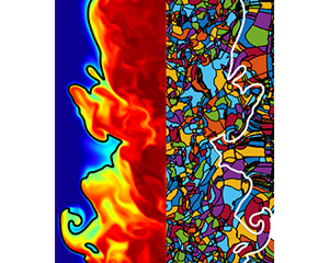
An entire field of DEs extracted from the intermediate  $\mathit {Re}$ case is shown in the top part of figure 7. The background field in this figure is that of the mixture fraction
 $Z$ in the
 $x$–
 $z$ centre plane of the turbulent jet, which is shown mirrored on the bottom part of the figure. The figure shows that dissipation elements are space-filling objects which subdivide the entire turbulent scalar field into smaller sub-units. As we follow the flame front indicated by the iso-line of the stoichiometric mixture fraction, we observe that DEs of various sizes and shapes are intersected by the flame. In addition, it can be seen that the size of the DEs increases as the core region of the jet is departed and the flame front is approached.
(a) DE analysis of the mixture fraction field of the intermediate  $\mathit {Re}$ case. Individual DEs are encompassed in a black contour. (b) Mirrored mixture fraction
 $Z$ field on which the DE analysis was performed. Blue colour indicates the oxidizer with
 $Z = 0$ and red the fuel
 $Z = 1$.

This observed increase in size has two reasons. Firstly, the increased diffusivity caused by the heat release as well as a mean relative velocity in the cross-stream direction cause the DE to increase in size. Secondly, the intersection area depicted here depends on the DE orientation with regard to the shown cut plane. DEs tend to be elongated tube-like structures, as seen in figure 6. Therefore, DEs oriented parallel to the  $x$–
 $y$ plane will appear significantly larger than DEs aligned with the spanwise direction. In the core of the jet, there is little to no preferential orientation of the DEs as the mixture fraction field is close to an isotropic state. However, crossing the reacting regions there are two reasons for a preferential orientation of the DEs. Due to the initialization and configuration of the cases with
 $Z = 1$ in the core and
 $Z = 0$ in the outer cross-stream position, it is more probable that the maxima are located closer to the core than the minima, which results in a natural alignment with the cross-stream direction. Additionally, the density differences cause a positive relative velocity between the extremal points spanning
 $Z_{{st}}$. On average, this relative velocity is the cross-stream component which further induces an orientation on the DEs in that direction.
In order to estimate the influence of small-scale turbulence in combustion, the local reaction layer thickness is typically compared to a turbulent length scale like the Kolmogorov scale  $\eta$. However, in non-premixed combustion, a comparison of the reaction layer thickness with turbulent length scales in physical space does not make much sense, because the width of the layer changes locally with the mixture fraction gradient. Since the transformation in mixture fraction space makes the flame structure more general, a meaningful comparison of scales, between the scalar difference
 ${\rm \Delta} Z$, provided locally by the individual DEs, with the reaction layer thickness
 $\delta Z_{r}$ is proposed. In this context, the DE parameter
 ${\rm \Delta} Z$ can be interpreted as the length in
 $Z$-space in which a flamelet-like solution can exist before terminating at its respective extremal points due to the influence of turbulence. Since the gradient trajectories used to identify individual DEs are identical to the physical coordinates of flamelets, DEs can also be viewed as groupings of flamelet solutions. As the flame thickness in non-premixed flames varies greatly with the mixture fraction gradient, a second parameter to characterize DEs is instrumental in the analysis. Characterizing the scalar gradient, the parameter
 $g = {\rm \Delta} Z / \ell$ will be used. Its square is expected to be related to the scalar dissipation rate
 $\chi$ as
 $\chi \sim D g^2$, as was observed in isotropic turbulence by Wang & Peters (Reference Wang and Peters2008).
4.1. Marginal dissipation element parameter statistics
One of the characteristic properties of DE parameters in non-reacting flows is the invariance of the probability density functions (PDFs) of the DE length  $\ell$ towards changes in Reynolds numbers and underlying scalar (Wang & Peters Reference Wang and Peters2008; Gampert et al. Reference Gampert, Schaefer, Goebbert and Peters2013a). When normalized by the mean DE separation length
 $\ell _{m}$, the PDFs of
 $\ell ^* = \ell / \ell _{m}$ show a characteristic shape and almost perfect agreement for the entire range of investigated Reynolds numbers. Figure 8 shows the PDFs of the normalized DE parameters for the four reacting cases and the two non-reacting jets. The PDFs were obtained from the final time steps in the respective simulations and weighted with the individual DE volumes. DEs whose minima are situated outside the TNTI, as obtained by the method of Bisset, Hunt & Rogers (Reference Bisset, Hunt and Rogers2002), were omitted from the statistics to rule out the inclusion of false extremal points in the laminar regions of the flows. In this fashion,
 $69.5\,\%$,
 $85.5\,\%$,
 $87.7\,\%$ and
 $92.1\,\%$ of the iso-surface of the stoichiometric mixture fraction is retained in the following statistics for the low
 $\mathit {Re}$ low dilution case, low
 $\mathit {Re}$ high dilution case, intermediate
 $\mathit {Re}$ case and high
 $\mathit {Re}$ case, respectively. The decreasing number of excluded DE with increasing Reynolds number is a strong indicator of the additional applicability of the method to flames with higher turbulence intensities.
Comparison of PDFs of the normalized DE length  $\ell / \ell _{{m}}$ (a) plotted in a linear scale and (b) logarithmic scale. (c) PDF of the normalized DE length conditioned on DEs crossing the stoichiometric iso-surface (with the black line obtained from (b), as a reference). (d) Ratio of the Kolmogorov micro-scale
 $\eta$ to the mean DE length
 $\ell _{m}$ for the investigated cases. The dash dotted line indicates the average ratio obtained from isotropic turbulence in Wang & Peters (Reference Wang and Peters2006). The line is placed arbitrarily as no jet Reynolds numbers exist.

In figures 8(a) and 8(b), the normalized DE length for all investigated cases is shown. The characteristic shape of the PDFs observed in the non-reactive cases is retained in the reacting simulations (Wang Reference Wang2009; Gampert et al. Reference Gampert, Goebbert, Schaefer, Gauding, Peters, Aldudak and Oberlack2011). After an initial steep linear increase for the shortest elements, a maximum of the PDFs is reached at approximately  $1.6 \ell ^*$. This linear increase was attributed to the diffusive drift of extremal points by Wang & Peters. After the maximum, a exponential decrease of the PDF for the longer elements follows, which stems from the random cutting and reconnection process of turbulent eddies (Wang & Peters Reference Wang and Peters2006). A perfect agreement is observed among all cases for the short elements. The wider separation of scales due to increasing Reynolds numbers is apparent in the tails of the PDFs which reach larger values for increasing Reynolds numbers. In figure 8(c), the PDF of the normalized DE length is conditioned on DEs which cross the iso-surface of the stoichiometric mixture fraction. Again, the PDFs display the characteristic course observed in the PDFs of the entire flow field. The mean DE length
 $\ell _{m}$ is only slightly larger (approximately
 $15\,\%$) compared to the one obtained for all DEs within the TNTI. These observations are a strong indication that the geometry of the flow and its reactive nature do not fundamentally change the characteristic length scale of turbulent structures identified by the DEs.
In figure 8(d), the ratio of the mean DE length and the Kolmogorov micro-scale is shown for all DEs within the TNTI. The scaling of  $\ell _{{m}}$ with
 $\eta$, which was already observed for other flow configurations, is also present in the reactive flows.
 $\ell _{{m}}/\eta$ is approximately constant for the wide range of Reynolds numbers and configurations investigated in this work and close to the ratio observed in the isotropic configurations. In particular, the average DEs length is approximately 25–35 Kolmogorov scales. The difference in ratio with regards to the isotropic turbulence might be attributed to the presence of shear in the jet configuration.
4.2. Joint dissipation element parameter statistics
Figure 9 shows the joint probability density functions (jPDF) of the normalized DE length  $\ell ^*$ and the normalized scalar difference
 ${\rm \Delta} Z^* = {\rm \Delta} Z / {\rm \Delta} Z_{m}$, with the volume-averaged scalar difference
 ${\rm \Delta} Z_{m}$, of the three jet cases in the final time step of the simulations. For the non-reacting cases in figures 9(a) and 9(b), one observes a global maximum of the probability density in the lower left corner for short elements and small scalar differences. This region of the jPDF is dominated by the diffusive drift of the extremal points leading to an annihilation of small DEs. On the top left-hand side, for small
 $\ell$ and big
 ${\rm \Delta} Z$, the probability of ramp-cliff structures, ubiquitously present in scalar turbulence, can be observed (Antonia & Sreenivasan Reference Antonia and Sreenivasan1977; Holzer & Siggia Reference Holzer and Siggia1994). These structures are linked to external and internal intermittency and manifest themselves in very steep gradients of the scalar followed by a very gradual decent. Likewise, the scalar dissipation rate
 $\chi$ displays extreme spatial fluctuations. The lower right part of the jPDF, for long elements and small scalar differences, shows the regime of the physical mechanism of splitting and reconnection of DEs (Wang & Peters Reference Wang and Peters2006). Qualitatively, the jPDFs of the two non-reactive cases agree.
The jPDF of the normalized DE length  $\ell ^* = \ell / \ell _{{m}}$ and normalized scalar difference
 ${\rm \Delta} Z^* = {\rm \Delta} Z/ {\rm \Delta} Z_{{m}}$ in the final time step of the respective cases. (a) Non-reacting case I, (b) non-reacting case II, (c) low
 $\mathit {Re}$ low dilution case, (d) low
 $\mathit {Re}$ high dilution case, (e) intermediate
 $\mathit {Re}$ case and (f) jPDF of the high
 $\mathit {Re}$ case.

The jPDFs of the reacting cases at low Reynolds number are shown in figures 9(c) and 9(d). Clear qualitative differences are observable compared to the non-reacting case. While the diffusive drift region of the lower part of the jPDF, for values of  ${\rm \Delta} Z^* < 0.8$ resembles its counterpart of the non-reacting flows, the top part looks vastly different. In addition to the local maximum probability in the diffusive drift region, the global maximum for intermediate
 $\ell$ and large
 ${\rm \Delta} Z$ is observed for the low
 $\mathit {Re}$ low dilution case. This indicates the high probability of DEs which span large mixture fraction differences almost all the way from the fuel to the oxidizer side. While the DE length distributions are unaffected by the chemical reactions, the statistics of
 ${\rm \Delta} Z$ are heavily influenced by chemical reactions and a distinct influence of the flame structure on the DE statistics can be observed. For the jPDF of the low
 $\mathit {Re}$ high dilution case, the global maximum shifts again into the diffusive drift region while the cliff structures imprinted by the flame remain more pronounced than in the non-reacting cases. These cliff structures become even less pronounced as the Reynolds number is increased in the intermediate
 $\mathit {Re}$ case in figure 9(e), where the second local maximum for large
 ${\rm \Delta} Z^*$ disappears. Finally, the jPDF of the high
 $\mathit {Re}$ case figure 9(f) completely resembles the jPDFs obtained from the non-reacting cases.
The (local) maximum probability density in figures 9(c) and 9(d) stems from insufficient turbulent mixing of the mixture fraction fields in these two cases. In the very beginning of the simulations, the mixture fraction fields have no turbulent fluctuations, and because of the lack of extremal points, all DEs would be infinitely long with  $\ell \rightarrow \infty$. Simultaneously, all gradient trajectories would reach from
 $Z =0$ to
 $Z =1$. Then, the DE difference would be uniformly
 ${\rm \Delta} Z = {\rm \Delta} Z_{m} = 1$. As turbulent mixing is applied to the mixture fraction fields, the turbulent eddies induce extremal points which reduce both
 $\ell$ and
 ${\rm \Delta} Z$ as time progresses. Diffusive drift will remove extremal points once elements are small enough. Therefore, the high probability of large
 ${\rm \Delta} Z$ (in other words, close to its initial value) is a result of either not enough time for the statistics
 ${\rm \Delta} Z$ to have fully converged at the end of the simulations, or the lack of sufficient turbulence to reach the asymptotic state observed in the non-reacting cases or in the High
 $\mathit {Re}$ case. The explanation for this is twofold. The locally high diffusivity in the reacting regions smooths the scalar field and removes more extremal points in these regions. In addition, the locally low effective Reynolds number causes lower eddy turnover times. Therefore, fewer extremal points are introduced in the reacting regions.
The difference in the jPDFs between the low Reynolds number reacting and non-reacting cases could therefore be attributed to low Reynolds number effects in the reacting cases, which is amplified by heat release. Similar results with regards to trends of the effects of heat release on small-scale statistics of the velocity and mixture fraction in non-premixed flames were reported in Attili & Bisetti (Reference Attili and Bisetti2019). Additionally, this is consistent with the findings of Gauding et al. (Reference Gauding, Dietzsch, Goebbert, Thévenin, Abdelsamie and Hasse2017), where a similar effect on the joint DE statistics conditioned on the flame front was observed. Likewise, the differences were linked to poor mixing in the reactive regions of the flow. This is another strong indicator that not only the marginal DE length statistics  $P(\ell )$, but also the DE scalar difference statistics of passive scalars in turbulent flows share a universal form if the Reynolds number is sufficiently high, regardless of the presence of combustion and heat release. Therefore, the differences between the jPDF of the DE parameters of a passive scalar field obtained from the reacting configurations and the universal form of the jPDF might be used to judge the extent of low Reynolds number effects.
For a more quantitative way to compare the DE statistics and to relate DE parameter statistics to a more commonly used method of analysis of turbulence, the mean of the normalized DE scalar difference is conditioned on the normalized DE length  $\langle {\rm \Delta} Z^* | \ell ^* \rangle$ and
 $\langle {\rm \Delta} \phi ^* | \ell ^* \rangle$, with
 $\langle \rangle$ indicating the average of all grid points within the TNTI. The
 $n$th conditional moment
 $\langle {\rm \Delta} \phi ^n | \ell ^* \rangle$ can be interpreted as an analogue of the conventional structure function (Wang & Peters Reference Wang and Peters2006)
 \begin{equation} S_n(r_i) = \langle(\phi (x + r_i) - \phi(x) )^n \rangle , \end{equation}
with  $r_i$ being the spatial separation between the two points. Therefore,
 $\langle {\rm \Delta} Z^* | \ell ^* \rangle$ and
 $\langle {\rm \Delta} \phi ^* | \ell ^* \rangle$ resemble a first-order moment of scalar difference across a distance
 $r_i$, i.e. the first-order structure function
 $S_1$. For isotropic turbulence
 $\langle {\rm \Delta} \phi ^* | \ell ^* \rangle$ was found to scale with Kolmogorov's
 $1/3$ power law (Wang Reference Wang2009; Gampert et al. Reference Gampert, Goebbert, Schaefer, Gauding, Peters, Aldudak and Oberlack2011). The mean of
 ${\rm \Delta} Z^*$ conditioned on
 $\ell ^*$ for the intermediate
 $\mathit {Re}$ for all DEs within the TNTI is shown in figure 10(a). One observes a clear correlation between the two DE parameters for short elements with
 $\ell ^* < 1$. The scaling exponent is significantly larger than the theoretically derived value. For larger elements, the two parameters appear to be less correlated. However, for the non-reactive case I as well as for the high
 $\mathit {Re}$ in figure 10(b), a good collapse of the conditional means and a clear scaling of
 $\langle {\rm \Delta} \phi ^* | \ell ^* \rangle$ for a wide range of
 $\ell ^*$ is observed. Thus, differences in the conditioned statistics of the intermediate
 $\mathit {Re}$ case can be attributed to low Reynolds number effects. The slightly larger scaling exponent displayed by the conditional means in figure 10(b), compared to the value usually observed in homogeneous isotropic turbulence, can be attributed to the presence of mean shear, as already observed in other non-reactive shear flows by Celani et al. (Reference Celani, Cencini, Vergassola, Villermaux and Vincenzi2005) and Attili & Bisetti (Reference Attili and Bisetti2013).
Normalized DE scalar difference conditioned on the normalized DE length  $\langle {\rm \Delta} Z^* | \ell ^* \rangle$ and
 $\langle {\rm \Delta} \phi ^* | \ell ^* \rangle$. The dashed line indicates the theoretically derived scaling.

An interesting observation is that the inertial range scaling can be observed for smaller scales in the conditional mean than in regular structure functions. This has also been reported by Wang & Peters (Reference Wang and Peters2006), who observed the analytic inertial range scaling of  $1/3$ in isotropic turbulence from scales as small as
 $7\eta$. Wang and Peters showed that in the vicinity of extremal points, the scalar field is more correlated. By using the conditional mean
 $\langle {\rm \Delta} Z^* | \ell ^* \rangle$, i.e. conditioning the structure functions on the monotonic regions in between the extremal points, this effect is significantly reduced and an inertial range scaling is observed at smaller scales.
In the flamelet regime, the scalar dissipation rate  $\chi$ serves as the parameter connecting the fields of the reactive species with the turbulent field, cf. (1.2) and (1.3). The correlation between the DE parameter and
 $\chi$ is therefore of high interest. Conveniently, the DE gradient
 $g = {\rm \Delta} Z/\ell$ can be used to relate the DE parameters to the scalar dissipation rate
 $\chi$. From dimensional considerations it follows that
 \begin{equation} \chi = 2 D \left( \frac{\partial Z}{\partial x_i}\right)^2 \sim Dg^2 . \end{equation}
The average ratio  $C_\chi = \langle \chi / ( 2 D g^2 )\rangle$ is shown for the last time step for all investigated cases in figure 11(a). Regardless of configuration and Reynolds number, the average ratio displays a constant value of
 $C_\chi \approx 5$. This indicates for the investigated configurations that the local mixture fraction gradient, and thus, the scalar dissipation rate, can indeed be related to the gradient of the larger local flow topology, as indicated by
 $g$. Further, the ratio of the second moment to the mean DE gradient squared
 $\langle g^2\rangle / g_{m}^2$ is shown in figure 11(b). No clear influence of Reynolds number is discernible and all cases display similar values for
 $\langle g^2\rangle / g_{m}^2 \approx 1.6$. The constant value for the ratio can be explained by the universality of the normalized jPDF
 $P(\ell ^*,{\rm \Delta} Z^*)$ and the consequently universal ratio of the various moments of
 $g = f(\ell ,{\rm \Delta} Z)$. Therefore, the mean scalar dissipation rate can be related to the mean DE gradient
 $\langle \chi \rangle \sim \langle D \rangle g_{m}^2$. Consequently, this signifies that the joint DE statistics can be reconstructed, if the unconditional mean scalar dissipation rate and Kolmogorov micro-scale are known.
(a) Average ratio  $C_\chi = \langle \chi / ( 2 D \langle g^2) \rangle$ in the final time step of the respective simulations. (b) Ratio of the first to the second moment of the DE scalar gradient
 $\langle g^2\rangle / g_{m}^2$. The dashed black line and black square indicate the isotropic turbulence.

5. Regimes in turbulent non-premixed combustion
5.1. Regime diagram
One of the desirable features of DEs is their space-filling nature, enabling a unique decomposition of the entire scalar field, and therefore, the ability to locally categorize the flame using the DE parameters. A categorization of combustion regimes based on DE parameters is outlined in this section. Similar to the Borghi–Peters regime diagram for turbulent premixed combustion, the turbulent scales are compared to the characteristic combustion scales. In the context of non-premixed combustion, the characteristic combustion scales are provided by the steady state flamelet solution. The DE parameter-based regime diagram and the expected flame structure or lack thereof is depicted in figure 12.
DE parameter based regime diagram for turbulent non-premixed combustion. The solid lines indicate a burning solution at  $Z_{{st}}$ and the dotted lines represent the thickness of the reaction zone.

The first DE parameter of choice is the gradient  $g$, as it is closely related to
 $\chi$, cf. figure 11(a). In the regime diagram, it represents the well-known and investigated influence of the scalar dissipation rate on the reacting scalars and is placed on the abscissa in figure 12. The first regime boundary is marked by the quenching gradient
 $g_{q}$, at which the heat release within the flame is insufficient to balance the energy transport caused by diffusion. In the flamelet sense,
 $g$ or
 $\chi$ should be sufficient to characterize the reacting scalars in flows with high but finite Damköhler numbers as outlined in Peters (Reference Peters2010). However, to account for the interaction of chemical and turbulent scales with Damköhler numbers approaching unity, a second parameter, represented by a second coordinate in the regime diagram, is required.
Representing the effect of the different turbulent scales in the mixture fraction field, the scalar difference  ${\rm \Delta} Z$ fills this spot and is therefore shown on the ordinate of the regime diagram in figure 12. The scalar difference
 ${\rm \Delta} Z$ is especially fitting, as the gradient trajectories used for the detection of DEs in the mixture fraction fields are linked to the local flamelet coordinates (Peters Reference Peters2009). The turbulence-induced extremal points in the mixture fraction field represent a forced interruption of any diffusive transport, as
 $\boldsymbol {\nabla } Z = 0$, or in the context of the flamelet equations (1.2) and (1.3),
 $\chi = 0$. The
 ${\rm \Delta} Z$ of a DE including the stoichiometric iso-surface is therefore the maximum distance in
 $Z$-space in which a diffusive transport-dominated structure, such as a flamelet, can exist. Therefore, the second boundary in the regime diagram is marked by the threshold value
 $Z$-space
 $({\rm \Delta} Z)_{t}$ below which the diffusive structure of the flame is disrupted too close to the stoichiometric mixture fraction, and thus the reaction zone, to form a coherent 1-D flame structure.
The result is the definition of four regimes. In the top left, for large  ${\rm \Delta} Z$ and small
 $g$, the ‘burning flamelet’ regime is situated. Regions of the flame identified by these DE parameters should adhere to the classical steady flamelet model. The scales in the turbulent
 $Z$-field are locally large compared to those imposed by the chemistry, and the individual flamelet solutions in the DE can advance unencumbered for long distances in
 $Z$-space, from the fuel side to the oxidizer. The DE gradient stays below quenching values ensuring a burning solution.
The regime in the top right corner, called the ‘large-scale extinction’ regime, corresponds to large-scale extinction events, such as large rollers stemming from Kelvin–Helmholtz instabilities and the like. Here, the specified ‘large scale’ is the characteristic scale of the extinction-inducing event, which is large compared to the scale indicated by the local DE. Within these regions, large cliff-ramp structures with significant strain are generated. Large-scale extinct regions such as flame holes (Lu & Ghosal Reference Lu and Ghosal2004; Pantano & Pullin Reference Pantano and Pullin2004) correspond to this regime. The extinction in this regime corresponds to the low Damköhler type extinction caused by eddies of integral scale size. The scale of the extinction events in this regime is expected to be far larger than the individual DE volumes, and the quenching process should occur fairly instantaneously and therefore homogeneously in a single DE.
The regime in the bottom left corner is the ‘fine-scale mixing’ regime, for  $g < g_{q}$ and
 ${\rm \Delta} Z < ({\rm \Delta} Z)_{t}$, is characterized by low gradients and small turbulent structures in the
 $Z$-field. This is indicative of very short flamelet solutions, and it is questionable if the chemical field in these regions resembles a one-dimensional solution or whether chemical reactions can be sustained. Low gradients and small scalar differences put these regions in the DE regime of ‘rapid splitting and reconnection’ (Wang & Peters Reference Wang and Peters2008), meaning that diffusive fluxes would rapidly change direction depending on the latest pairing of the extremal points in the DE. A flame structure in the traditional sense should not exist in the regions of ‘fine-scale mixing’ if
 ${\rm \Delta} Z$ is small enough and intense turbulent advection becomes the dominating transport mechanism. If the scalar difference is further decreased
 ${\rm \Delta} Z < \delta Z_{r}$, with the thickness of the reaction zone in
 $Z$-space
 $\delta Z_{r}$, DEs may penetrate the reaction zone and exist entirely in the reaction zone. The local topology of the flame would be more akin to homogeneous reactors than flamelets.
The last remaining regime is the ‘broken reaction zone’ regime in the bottom right corner. Here one finds small scalar differences in combination with large gradients leading to small-scale extinction zones due to locally high turbulence activity. This type of extinction would correspond to a high Karlovitz-type effect, where eddies of the size of the Kolmogorov-scale transport radicals out of the inner reaction zone. Contrary to the ‘large-scale extinction’ regime, the scales of the ‘broken reaction zone’ quenching events are far smaller. Consequently, quenching would not occur homogeneously within an entire DE resulting in partially burning DEs. The resulting local topology would be characterized by small intermittent pockets of reacting and non-reacting fluid.
In a first step, to ensure that DEs represent a sensible way of decomposing the physical space into sub-units for the purpose of analysing the interaction between chemistry and turbulence, the PDF of temperature conditioned on the mixture fraction  $P(T|Z)$ is compared to the conditional PDF of the DE-averaged temperature
 $\tilde {T}_{{\textrm {DE}}}$. This average is calculated in the following way. The intersecting area of the individual DEs and the
 $Z$ iso-surface is determined and the temperature in this intersecting area is then averaged. For
 $P(\tilde {T}_{{\textrm {DE}}}| Z)$, this intersecting area additionally serves as a weight in the statistics to account for the various sizes of the DEs. The PDFs of the instantaneous temperature and the DE-averaged temperature are shown in figure 13 for the low
 $\mathit {Re}$ low dilution case and intermediate
 $\mathit {Re}$ case for three exemplary values of the mixture fraction. One observes a characteristic bimodal shape of the PDFs for most of the
 $Z$ values, with the maximum at low temperatures corresponding to the extinct regions of the iso-surface and the maximum at high
 $T$ corresponding to the burning solution. No differences between the PDFs of the temperature and the DE-averaged temperature can be observed. These results are indicative of the fact that the flow compartmentalization by means of DEs is indeed sensible, as the full PDF can be reconstructed from the DE-averaged temperature with negligible errors.
The (solid lines): PDFs of the temperature  $P(T|Z)$ conditioned on three different values of the mixture fraction and (dashed lines): PDF of the temperature averaged within individual DEs
 $P(\tilde {T}_{{\textrm {DE}}}|Z)$. Red:
 $Z = 0.5 Z_{{st}}$, blue:
 $Z = Z_{{st}}$ and yellow:
 $Z = 1.5 Z_{{st}}$, (a) low
 $\mathit {Re}$ low dilution case, (b) intermediate
 $\mathit {Re}$ case.

The categorization based on the proposed regime diagram in figure 12 is applied to the surface of the stoichiometric mixture fraction of the four reacting cases. The quenching gradient is estimated by using the conditional average of the DE gradient at the scalar dissipation corresponding to quenching conditions for the laminar 1-D flamelet  $g_{q} = \langle g | \chi = \chi _{q} \rangle$. This results in a quenching gradient for the low
 $\mathit {Re}$ low dilution case of
 $g_{q} = 110\ \textrm {s}^{-1}$, while it is
 $g_{q} = 92\ \textrm {m}^{-1}$,
 $g_{q} = 89\ \textrm {m}^{-1}$ and
 $g_{q} = 90\ \textrm {m}^{-1}$ for the low
 $\mathit {Re}$ high dilution case, intermediate
 $\mathit {Re}$ case and high
 $\mathit {Re}$ case, respectively. The reaction thickness
 $\delta Z_{{r}}$ in
 $Z$-space is estimated locally by fitting the inner reaction zone of the heat release profile
 $\omega _T(Z)$ of the steady state flamelet solution with a Gaussian profile. The reaction zone thickness is then defined as the half-width of the Gaussian. This procedure is shown for conditions close to quenching for the two investigated dilutions in figure 14(a). For local dissipation rates greater than the quenching dissipation rate, the reaction zone thickness at quenching conditions is chosen. The impact of the scalar dissipation rate at stoichiometric conditions on the reaction zone thickness is shown in figure 14(b), where an approximately
 $60\,\%$ wider
 $\delta Z_{{r}}$ for the high dilution cases is observed.
(a) Heat release rate  $\omega _T$ for steady state flamelet solutions at quenching scalar dissipation rates (solid lines) and the inner reaction zone approximation by means of a Gaussian profile (dashed lines). Blue: low dilution corresponding to the boundary conditions in the low
 $\mathit {Re}$ low dilution case, green: boundary conditions corresponding to the low
 $\mathit {Re}$ high dilution case, the intermediate
 $\mathit {Re}$ case and the high
 $\mathit {Re}$ case. (b) Variation of the inner reaction zone thickness
 $\delta Z_{{r}}$ with
 $\chi _{{st}}$.

The reacting scalars on the iso-surface of the stoichiometric mixture fraction are averaged conditioned on the normalized DE parameters  ${\rm \Delta} Z' = {\rm \Delta} Z / \delta Z_{r}$ and
 $g' = g / g_{q}$ to achieve a comparison between the chemical and turbulent scales and check the validity of the proposed regime diagram. This is shown for the temperature field for all reacting cases in figure 15 and for the OH mass fraction in figure 16. The conditional means of the reacting scalars display a good consistency with the assumptions of the previously outlined DE-based regime diagram. For all four cases, high values of the conditional means
 $\langle T \rangle$ and
 $\langle Y_{\mathrm {OH}} \rangle$ are observed for high values of
 ${\rm \Delta} Z'$ and low values of
 $g'$, which is consistent with the idea of classifying the flame as burning flamelets for these values of DE parameters. Here, the reacting scalars display the same trends with regards to rising
 $g'$ as one would expect with an increase in
 $\chi$. The second regime boundary is set as
 $({\rm \Delta} Z)_{t} = 15 {\rm \Delta} Z'$, as the conditioned reacting scalar values decrease significantly. This value for
 ${\rm \Delta} Z'$ is consistent across all Reynolds numbers and across the different dilutions. The reacting scalars are more susceptible to quenching caused by gradients in the mixture fraction field for
 ${\rm \Delta} Z < ({\rm \Delta} Z)_{t}$, as similar values of
 $g$ yield significantly lower values of the mean reacting scalars.
Mean temperature  $\langle T \rangle$ conditioned on normalized DE parameters
 ${\rm \Delta} Z' = {\rm \Delta} Z / \delta Z_{r}$ and
 $g' = g / g_{q}$. Dashed lines indicate regime boundaries. (a) Low
 $\mathit {Re}$ low dilution case, (b) low
 $\mathit {Re}$ high dilution case, (c) intermediate
 $\mathit {Re}$ case and (d) high
 $\mathit {Re}$ case.

Mean OH mass fraction  $\langle Y_\textrm {{OH}} \rangle$ conditioned on normalized DE parameters
 ${\rm \Delta} Z'$ and
 $g'$. Dashed lines indicate regime boundaries. (a) Low
 $\mathit {Re}$ low dilution case, (b) low
 $\mathit {Re}$ high dilution case, (c) intermediate
 $\mathit {Re}$ case and (d) high
 $\mathit {Re}$ case.

The regime boundary at  $g' = 1$ proves to be sensible as well with low values of the mean reacting scalars indicating extinction for
 $g' > 1$. The locally high values for
 $\langle T \rangle$ and
 $\langle Y_{\mathrm {OH}} \rangle$ in the ‘large scale extinction’ regime, present only in the low
 $\mathit {Re}$ case and intermediate
 $\mathit {Re}$ case, are not present in the high
 $\mathit {Re}$ case and can be attributed to the aforementioned low Reynolds number effects which cause
 $g$ and
 $\chi$ to be locally less correlated. The range of values of the normalized DE parameters
 ${\rm \Delta} Z'$ and
 $g'$ observed in the individual cases and the implied regime contributions to the overall combustion is consistent with the probability of observing small-scale structures in the flame and extinct regions in figure 4 and the overall levels of extinction in figure 5.
The fine-scale regimes ‘fine-scale mixing’ and ‘broken reaction zones’ are characterized by small structures in mixture fraction space and display highly turbulent behaviour. To gain a deeper understanding of the fine-scale mixing regimes, the mean temperature in the extremal points, i.e. at the minimum mixture fraction,  $\langle T_{{\textrm {DE},min}} \rangle$, and at the maximum mixture fraction,
 $\langle T_{{\textrm {DE},max}} \rangle$, of the DEs crossing the iso-surface is conditioned on the normalized DE parameters as shown in figure 17. High values for the mean temperature in the extremal points can be observed in a triangular region for
 ${\rm \Delta} Z' < 10$ and
 $g' < 1$. The values of the mean reacting scalars are comparable to those obtained at the stoichiometric iso-surface, as observed for the small
 ${\rm \Delta} Z'$ and
 $g'$ in figures 15 and 16. The presence of extremal points of the mixture fraction field within the reaction zone further validates the idea of a ‘fine-scale mixing’ regime. The DEs in this regime resemble fully reacting sub-regions of the flame from the minimum to maximum.
Mean temperature (a) in the minima  $\langle T_{{\textrm {DE},min}} \rangle$ and (b) in the maxima
 $\langle T_{{\textrm {DE},max}} \rangle$ of DEs crossing the stoichiometric iso-surface conditioned on the normalized DE parameter
 $g'$ and
 ${\rm \Delta} Z'$ for the high
 $\mathit {Re}$ case. The dashed lines indicate the regime boundaries.

Due to the small  $g'$ in this triangular region, the
 $\ell$ of the DE occupying this part of the flame ranges from
 $5 \eta < \ell < 50 \eta$. This indicates the presence of large and fully reacting structures, which are significantly wider than the reaction zones in the flamelet solution. The values of
 $10 < {\rm \Delta} Z' < 15$ might be viewed as a transition range between two burning regimes.
For a final analysis of the sensibility of the DE-based regime diagram and to estimate the level of extinction in the individual regimes, the marginal PDF of the temperature at stoichiometric conditions  $P(T_{{st}})$ is additionally conditioned on the individual combustion regimes. This is shown for two time steps for the high
 $\mathit {Re}$ case in figure 18. As observed in figure 13(b), two peaks in the PDFs are present, one for low temperatures and one for high temperatures corresponding to burning and extinct parts of the stoichiometric iso-surface, respectively. For the extinction regimes, the global maximum of the probability density is located at low temperatures with only minor amounts in temperature ranges that can sustain combustion. The remaining low amounts of probability density of low temperature in the ‘burning flamelets’ regime can be explained by parts of the flow undergoing re-ignition or by locally too high values of
 $\chi$ for re-ignition of previously extinguished parts of the flow.
PDF of the temperature conditioned on the stoichiometric mixture fraction, and on the individual regimes in the final time step of the high  $\mathit {Re}$ case.

5.2. Local flame analysis
As the gradient trajectories in mixture fraction space are equivalent to the physical coordinates of the flamelet solution in physical space, a non-local comparison with the steady state flamelet solution in a physically meaningful framework is straightforward. For a more detailed investigation, the instantaneous mass fraction of OH obtained along all gradient trajectories used in the detection of exemplary DEs are plotted in the mixture fraction space in figure 19. This is done for three representative DEs obtained from the ‘burning flamelet’ regime, the ‘fine-scale mixing’ regime and the ‘broken reaction zone’ regime in the last time step of the high  $\mathit {Re}$ case. The representative DEs are obtained from burning regions of the stoichiometric iso-surface, as shown in figure 5. The DEs are of comparable volume and possess a similar intersecting area with the iso-surface of the stoichiometric mixture.
 $Y_\textrm {{OH}}$ along the gradient trajectories is compared to the steady state flamelet solutions obtained from the steady state flamelet solution using the averaged scalar dissipation rate at the intersecting area of the DE and the stoichiometric mixture fraction iso-surface
 $\widetilde {\chi _{{st}}}_{{\textrm {DE}}}$.
The (grey lines) mass fraction of OH radicals obtained along all gradient trajectories of a single DE. The steady state flamelet solution for the DE-averaged scalar dissipation rate at stoichiometric conditions  $\widetilde {\chi _{{st}}}_{{\textrm {DE}}}$ is indicated by the blue dashed line and red dashed line for the non-unity Lewis number and unity Lewis number solutions, respectively. (a) DE obtained from the ‘burning flamelet’ regime, (b) DE from the ‘fine scale mixing’ regime and (c) DE obtained from the ‘broken reaction zones’ regime.

For the DE obtained from the ‘burning flamelet’ regime, shown in figure 19(a), the mass fractions along the individual trajectories collapse perfectly with the unity  $\mathit {Le}$ flamelet solution for a wide range of
 $Z$ values. The indiscernibility of
 $Y_\textrm {{OH}}$ between the individual trajectories is very consistent with the flamelet assumption of a change of any reactive scalar exclusively in the
 $Z$-direction. However, for the DE obtained from the ‘fine-scale mixing’ regime in figure 19(b),
 $Y_\textrm {{OH}}$ displays a wide range of values for a given value of
 $Z$, especially for mixture fractions close to stoichiometry. Large departures from both flamelet solutions can be observed with
 $Y_\textrm {{OH}}$ obtained in the DE having consistently higher values, even in the extremal points. The rather large inhomogeneity of the reacting scalar on an iso-surface of
 $Z$ within a small spatial sub-unit, such as a DE, clashes with the 1-D flamelet assumption, as additional transport of the reacting scalars is expected to take place tangentially to the mixture fraction coordinate. The mass fraction of OH obtained from the ‘broken reaction zones’ regime, shown in figure 19(c) shares this characteristic. While the range of values is significantly larger than in the DEs of the other regimes, some trajectories display values corresponding to an extinct solution while others are fully burning, which is consistent with the assumption of a ‘broken reaction zones’ regime.
The effect of the inhomogeneity of reactive scalars for a specific iso-value of  $Z$, which is observed for the exemplary DEs in the ‘fine-scale mixing’ regime and ‘broken reaction zones’ regime, can be statistically measured by the coefficient of variation of a reactive scalar in a DE
 \begin{equation} c_{{v,\alpha}}(Z) = \frac{\sqrt{\widetilde{\psi''^2}_{\alpha,{\textrm{DE}}}(Z)}}{\tilde{\psi}_{\alpha,{\textrm{DE}}}(Z)} . \end{equation}
The mean coefficient of variation of OH at stoichiometry, conditioned on the normalized DE parameters  $\langle c_{{v,\mathrm {OH}}}(Z_{{st}}) | g', {\rm \Delta} Z' \rangle$, is shown for the low
 $\mathit {Re}$ high dilution case and the intermediate
 $\mathit {Re}$ case in figures 20(a) and 20(b). The coefficient of variation is low in the ‘burning flamelet’ regime for both cases and is also relatively low for the ‘large scale extinction’ regime. As partly quenched DEs would display high values of the coefficient of variation, the low values support the notion of larger extinction events where regions spanning the entire cross-section of the DE are quenched simultaneously. High values for the coefficient of variation are observed in both the ‘fine-scale mixing’ regime and the ‘broken reaction zones’ regime. This indicates that the previously observed characteristics for the three exemplary DEs in figures 19(a)–19(c) are representative of the entire flame.
Mean DE coefficient of variation of the OH mass fraction  $\langle c_{{v,\mathrm {OH}}}(Z_{{st}}) \rangle$ conditioned on the normalized DE parameters
 $g'$ and
 ${\rm \Delta} Z'$ at the final time step. (a) Low
 $\mathit {Re}$ high dilution case; (b) intermediate
 $\mathit {Re}$ case; (c) PDF of the DE coefficient of variation
 $P(c_{{v,\mathrm {OH}}}(Z_{{st}}) )$ conditioned on the individual regimes in the burning regions of the stoichiometric iso-surface for the high
 $\mathit {Re}$ case.

The PDF of the coefficient of variation of the temperature  $P(c_{{v,}T}(Z_{{st}}))$ conditioned on the individual regimes and the burning regions of the high
 $\mathit {Re}$ case is shown in figure 20(c). It shows that previously observed behaviour of the coefficient of variation with regard to the regimes extends to the temperature field. The difference in
 $c_{{v,}T}$ between the large-scale and the fine-scale regimes is approximately one order of magnitude. While comparable to the ‘large scale extinction’ regime, the ‘burning flamelet’ regime displays the lowest
 $c_{{v,}T}$. In summary, independent of the value of
 $g$, the reacting scalar fields display high local homogeneity in the ‘burning flamelet’ regime and ‘large-scale extinction’ regime, while the ‘fine-scale mixing’ regime and the ‘broken reaction zones’ regime are characterized by turbulence-induced inhomogeneity.
5.3. Temporal evolution of the combustion regimes
Finally, the temporal evolution of the individual regime's contribution to the overall combustion process is investigated. Besides offering  ${\rm \Delta} Z$ as a value to quantify ‘large-scale’ or ‘fine-scale’ interaction, the approach of using DE parameters for a classification of the combustion regimes offers a significant additional advantage over traditional statistical methods. Instead of comparing one single characteristic turbulence scale, which is defined for the entire domain (like the Kolmogorov micro-scale
 $\eta$ in the Karlovitz number or the eddy turnover time
 $\tau$ in the Damköhler number) to the characteristic flame scale, a local comparison using DE parameters is possible. Every material point on the stoichiometric iso-surface can be characterized by the two DE parameters. Therefore, all of these material points can be classified individually by the DE-based regime diagram. The large range of turbulent structures simultaneously present in the various cases consequently leads to a certain degree of coexistence of combustion regimes in the conditions investigated in this work. The substantial advantage of using a local estimate for the turbulence scales allows for the quantification of the local conditions. For the coexistence of burning and extinct regimes, this was always implicitly assumed by the simultaneous presence of flame holes and edge flames in flows for which the average scalar dissipation rate remained well below quenching values (Lignell et al. Reference Lignell, Chen and Schmutz2011; Attili et al. Reference Attili, Bisetti, Mueller and Pitsch2015).
To achieve the local quantification of the combustion regimes, the burning area of the stoichiometric iso-surface attributed to the individual regimes in the burning regions of the flow  $A_{i,{st,burn}}(t^*)$ is shown for all four reacting cases in figure 21(a). As the overall burning area increases significantly over time, normalization is achieved with the overall burning area
 $A_{{st,burn}}(t^*)$, which is identical to the one shown in figure 5(b).
Temporal evolution of the normalized area of the stoichiometric iso-surface attributed to the individual regimes  $A_{i,{burn}}^* = A_{i,{st,burn}}(t^*) / A_{{st,burn}}(t^*)$, conditioned on the burning regions. (a) Solid lines indicate the ‘burning flamelet’ regime and dashed lines the ‘fine-scale mixing’ regime. (b) Dash-dotted lines indicate the ‘large scale extinction’ regime and dotted lines the ‘broken reaction zones’ regime.

As expected, the combustion is classified as the ‘burning flamelet’ regime in the early time steps of all four cases. Later, the burning regions are almost completely classified as either ‘burning flamelet’ regime or ‘fine-scale mixing’ regime. The relative contribution of the ‘fine-scale mixing’ regime increases with the higher dilution and the higher Reynolds number. While the ‘burning flamelet’ regime and the ‘fine scale mixing’ regimes possess roughly the same area in the last time step of the intermediate  $\mathit {Re}$ case, the ‘fine scale mixing’ regime is the dominant regime in the final time step of the high
 $\mathit {Re}$ case.
The temporal evolution of the normalized area of the stoichiometric iso-surface in the burning regions attributed to the ‘large-scale extinction’ regime and the ‘broken reaction zones’ regime is shown in figure 21(b). Consistent with the assumption of the regimes, the areas of both the ‘large-scale extinction’ regime and the ‘broken reaction zones’ regime are very low in the burning regions, which is emphasized by the significantly lower range of values on the ordinate. Consequently, the overall contributions of the two regimes to the stoichiometric iso-surface in the burning regions in the final time step ranges from  $0\,\%$ for the low dilution low
 $\mathit {Re}$ case to only
 $7\,\%$ in the high
 $\mathit {Re}$ case.
The burning area in the two regimes might be attributed to ongoing extinction events in these time steps and is well correlated with the point in time, as well as with the ratio of burning regions of the stoichiometric iso-surface to the overall stoichiometric iso-surface, cf. figure 5(b). The area of the ‘large scale extinction’ regime is approximately the same for all three high dilution cases, which can be attributed to the comparable value of the Damköhler numbers. However, the temporal evolution of the area of the ‘broken reaction zones’ shows a clear dependence on the Reynolds numbers.
6. Conclusions
The DE analysis was applied to the mixture fraction fields and passive scalar fields of six reacting and inert 3-D DNS of the temporally evolving jet configuration. The statistics of the normalized DE parameter  $\ell ^*$ showed the characteristic invariance towards changes in Reynolds numbers and was unaffected by the heat release in the reacting cases. The mean DE length
 $\ell _{m}$ was found to scale with the Kolmogorov micro-scale. The effect of the heat release on the DE scalar difference
 ${\rm \Delta} Z$ was observed, with an increased probability of cliff-ramp structures in the mixture fraction field. However, the effect of the heat release on the statistics decreased with an increasing dilution of the fuel stream and with an increase in the Reynolds number. The jPDF of the two normalized DE parameters obtained from the highest Reynolds number reacting case displayed the universal form observed in the non-reacting cases. DE parameter statistics were related to structure functions and the correlation between the DE gradient
 $g$ and the scalar dissipation rate
 $\chi$ was demonstrated. This correlation allows for the reconstruction of the DE parameter statistics from the value of the unconditional scalar dissipation rate.
Additionally, a DE parameter-based regime diagram was introduced. The DE parameters  $g$ and
 ${\rm \Delta} Z$ were compared to flame scales with the quenching gradient
 $g_{q}$ and the reaction zone thickness
 $\delta Z_{r}$ for a local classification of the flame front into four regimes. The regime assumptions were tested employing the correlation between DE parameters and reacting scalars on a non-dimensional basis. The soundness of the regime diagram was shown for all four reacting cases. Below the regime threshold value of
 ${\rm \Delta} Z \leq ({\rm \Delta} Z)_{t} = 15 \delta Z_{r}$ the model assumptions of a 1-D flamelet cease to be valid as the reacting scalars display gradients in the tangential direction to the flamelet coordinates in physical space. Above this threshold value, the local conditional fluctuations of the reacting scalars are small, irrespective of the value of dissipation rate. The temporal evolution of contribution of the combustion regimes to the overall combustion was consistent with both the conventional turbulent flame analysis and the qualitative appearance of the flames in the four reacting cases.
Acknowledgements
The authors gratefully acknowledge funding from of the Deutsche Forschungsgemeinschaft (DFG) Project PE 241/441. Further, the authors gratefully acknowledge the Gauss Centre for Supercomputing e.V. (www.gauss-centre.eu) for funding this project by providing computing time on the GCS Supercomputer JUWELS at Jülich Supercomputing Centre (JSC).
Declaration of interests
The authors report no conflict of interest.



