1 Introduction
The drag force on a sphere in a steady flow is well established and dates back to the work of Stokes (Reference Stokes1851). He considered both the steady and time-harmonic motion of a sphere in a quiescent incompressible fluid and obtained an expression for force in the frequency domain. When the flow or the spherical particle motion is unsteady, the force expression in the time domain, which includes the unsteady added-mass and viscous-history effects, was provided by Boussinesq (Reference Boussinesq1885), Basset (Reference Basset1888) and Oseen (Reference Oseen1927) (now known as the BBO equation).
The above investigations assumed the undisturbed ambient flow in the absence of the particle to be spatially uniform and as a result, all spatial inhomogeneity is due to the disturbance field created by the particle and its relative motion with respect to the uniform ambient flow. For a spatially non-uniform undisturbed ambient flow, Faxén (Reference Faxén1922) provided a remarkably simple and elegant result to compute the steady-state drag. The resulting force expression is identical to the formula of Stokes (Reference Stokes1851), with the uniform flow velocity replaced by the undisturbed non-uniform ambient velocity averaged over the particle surface. In the incompressible limit, the transient force on the particle in a spatially inhomogeneous ambient flow in the frequency domain was obtained by Mazur & Bedeaux (Reference Mazur and Bedeaux1974). The corresponding explicit expression for force in the time domain was presented by Gatignol (Reference Gatignol1983) and Maxey & Riley (Reference Maxey and Riley1983). The resulting (MRG) equation can be considered as an extension of the Faxén theorem to the BBO equation.
The effects of compressibility in the particle equation of motion were introduced in the pioneering work of Zwanzig & Bixon (Reference Zwanzig and Bixon1970). Similar results were also reported (Guz Reference Guz2009) by solving the linearized Navier–Stokes equation in the frequency domain. In a recent work, Parmar, Haselbacher & Balachandar (Reference Parmar, Haselbacher and Balachandar2011) presented a compressible version of the BBO equation in the time domain (denoted PHB in this paper). It should be emphasized that although both compressibility and unsteady effects were included in Zwanzig & Bixon (Reference Zwanzig and Bixon1970), Guz (Reference Guz2009), Parmar et al. (Reference Parmar, Haselbacher and Balachandar2011), the undisturbed ambient flow was still treated to be spatially uniform.
There are many applications, such as propagation of a shock wave over a finite-sized particle, where the undisturbed ambient flow seen by the particle is both inhomogeneous (spatially varying on the scale of the particle) and time dependent. Furthermore, in such cases the compressibility of the ambient fluid flow becomes important. One of the earliest work accounting for non-uniform ambient viscous flows in a compressible medium was carried out by Bedeaux & Mazur (Reference Bedeaux and Mazur1974) and their analysis was in the frequency domain. In applications involving particle-laden flows, we desire to track the trajectories of individual particles over time through complex time-dependent flows. In these situations it is important to go beyond the frequency-domain description and obtain an explicit expression for the force in the time domain. Recently Parmar, Haselbacher & Balachandar (Reference Parmar, Haselbacher and Balachandar2012) obtained an explicit force expression in the time domain applicable to the arbitrary motion of a particle in an unsteady inhomogeneous ambient flow, closely following the works of Gatignol (Reference Gatignol1983) and Maxey & Riley (Reference Maxey and Riley1983). The linearization process in the above analyses restricted the Reynolds and the Mach numbers (based on particle diameter and relative velocity) to be small, but also required the particle to be smaller than the length scales of ambient flow variation. It should be noted that Faxén’s law for the steady Stokes flow did not requite this latter restriction on the size of the particle. Thus, the results of Gatignol (Reference Gatignol1983), Maxey & Riley (Reference Maxey and Riley1983) and Parmar et al. (Reference Parmar, Haselbacher and Balachandar2012) are unsteady generalizations of the Faxén law in a restricted sense. In particular, the results of Parmar et al. (Reference Parmar, Haselbacher and Balachandar2012) will not strictly apply to cases where the particle size is comparable to the wavelength of the acoustic field, or to the problem of shock–particle interaction, since shock thickness is typically much smaller than the particle size.
The primary objective of this article is to obtain the Faxén’s form of the force expression in the time domain for a spherical particle subjected to an unsteady inhomogeneous compressible flow, without a strong limit on the size of the particle compared to the length scales of the inhomogeneous ambient flow. In pursuit of this goal, we consider the classic problem of a plane travelling wave of given frequency and wavelength,
 $\unicode[STIX]{x1D706}$
, passing over a rigid sphere of radius,
 $R$
, situated in an otherwise viscous compressible quiescent ambient. Following traditional analysis in the acoustic literature (Hasegawa & Yosioka Reference Hasegawa and Yosioka1969; Doinikov Reference Doinikov1994; Guz Reference Guz2009), the flow velocity is expressed as a summation of scalar and vector potentials (Lamb Reference Lamb1993) known as Helmholtz decomposition, and on application of the no-slip boundary condition on the particle surface, the desired force expression is obtained in the frequency domain as a complex drag coefficient (or inverse mobility coefficient). This result is identical to that obtained by Bedeaux & Mazur (Reference Bedeaux and Mazur1974), where the authors computed the force using the method of induced forces.
The quest then is to transform this result to the time domain and appropriately decompose the total force into physically meaningful terms such as the undisturbed force, quasi-steady, inviscid-unsteady and viscous-unsteady components as in Parmar et al. (Reference Parmar, Haselbacher and Balachandar2012). Based on the MRG equation, in the time domain we expect the force expression to be an integro-differential equation that involves surface (and volume) averages of the inhomogeneous undisturbed ambient flow over the location of the particle. Note that the wavenumber and frequency of the acoustic field are related by the speed of sound. Thus, separation of the complex drag coefficient into wavenumber and frequency components and their subsequent transformations to time domain and spatial averages is the key aspect of the derivation to be presented. Here we use the results of Parmar et al. (Reference Parmar, Haselbacher and Balachandar2011, Reference Parmar, Haselbacher and Balachandar2012) as guidance to accomplish this separation and thereby obtain the force expression in the Faxén form that is applicable for arbitrary unsteady viscous compressible flows over a sphere. The results obtained are similar to those presented in Parmar et al. (Reference Parmar, Haselbacher and Balachandar2012), where the authors approached the problem using Lorentz reciprocal theorem (Landau & Lifschitz Reference Landau and Lifschitz1987). The formulation of Parmar et al. (Reference Parmar, Haselbacher and Balachandar2012) allowed for any arbitrary ambient flow that varied on a length scale
 $\unicode[STIX]{x1D706}$
and the linearization process required both the Reynolds number based on relative velocity to be small (i.e.
 $U_{rel}R/\unicode[STIX]{x1D708}\ll 1$
) and a restriction on particle size (i.e.
 $R/\unicode[STIX]{x1D706}\ll 1$
). In the present analysis by restricting attention to a small amplitude acoustic wave propagating over a particle in an otherwise quiescent medium we only require
 $U_{rel}R^{2}/(\unicode[STIX]{x1D708}\unicode[STIX]{x1D706})\ll 1$
. Thus provided Reynolds number is sufficiently small the present results apply even to particles of diameter
 $d$
larger than the wavelength
 $\unicode[STIX]{x1D706}$
.
We test the Faxén form of the force by applying it to the case of a one-dimensional expansion fan interacting with a stationary particle. First we consider the weak case where the velocity jump across the expansion fan (from head of the expansion fan to the tail of the expansion fan) is infinitesimally small. When applied to this case of a weak expansion fan, where linear approximation applies, we observe that the prediction compares precisely with those from the corresponding direct numerical simulation. We also consider an expansion fan of finite strength where the velocity across the fan jumps from zero to Mach
 $0.35$
and compare the theoretical prediction against numerical simulations. In the specific example to be considered, the thickness of the expansion fan when it first encounters the particle is
 $0.6$
times the particle radius. Thus the length scale of the undisturbed ambient flow is of the order of the particle size. When we account for the nonlinear effects by transforming the local time derivatives to substantial time derivatives, we accurately predict the drag force.
The paper is organized as follows. Section 2 discusses the acoustic analogy used in obtaining the force on a particle due to a plane wave of a given frequency and wavenumber in terms of scattering coefficients. The transformation to the time domain is discussed in detail in § 3 and the extension of Faxén’s theorem to nonlinear flows is analysed in § 4. A summary of Faxén’s equation of motion for spatially varying unsteady viscous compressible flows and its reductions to a variety of limiting cases such as standard Faxén, compressible and incompressible BBO and MRG equations is tabulated in § 5. The force expression derived in this study applied to predict the force on a finite-sized particle due to interaction with a planar expansion fan is presented in § 6. The Faxén force equation as applicable to moving particles is discussed in § 7, followed by the conclusions of our study in § 8.
2 Acoustic solution
We start with the classical problem of an incident planar sound wave in a viscous compressible, but otherwise stationary, medium scattered by a spherical particle of finite radius. The incident and the disturbance fields are described by the compressible Navier–Stokes equations:
 $$\begin{eqnarray}\displaystyle & \displaystyle {\displaystyle \frac{\unicode[STIX]{x2202}\unicode[STIX]{x1D70C}}{\unicode[STIX]{x2202}t}}+\unicode[STIX]{x1D735}\boldsymbol{\cdot }(\unicode[STIX]{x1D70C}\boldsymbol{u})=0, & \displaystyle\end{eqnarray}$$
 $$\begin{eqnarray}\displaystyle & \displaystyle {\displaystyle \frac{\unicode[STIX]{x2202}(\unicode[STIX]{x1D70C}\boldsymbol{u})}{\unicode[STIX]{x2202}t}}+\unicode[STIX]{x1D735}\boldsymbol{\cdot }(\unicode[STIX]{x1D70C}\boldsymbol{u}\boldsymbol{u})=\unicode[STIX]{x1D735}\boldsymbol{\cdot }\unicode[STIX]{x1D748}, & \displaystyle\end{eqnarray}$$
where,
 $\unicode[STIX]{x1D748}$
is the stress tensor defined as:
 $$\begin{eqnarray}\displaystyle \unicode[STIX]{x1D748}=[-p\boldsymbol{I}+\unicode[STIX]{x1D707}(\unicode[STIX]{x1D735}\boldsymbol{u}+(\unicode[STIX]{x1D735}\boldsymbol{u})^{\text{T}})+(\unicode[STIX]{x1D707}_{b}-{\textstyle \frac{2}{3}}\unicode[STIX]{x1D707})(\unicode[STIX]{x1D735}\boldsymbol{\cdot }\boldsymbol{u})\boldsymbol{I}]. & & \displaystyle\end{eqnarray}$$
The flow is assumed to be isentropic and hence the pressure depends only on density as:
 $$\begin{eqnarray}\displaystyle p=p(\unicode[STIX]{x1D70C}). & & \displaystyle\end{eqnarray}$$
In the above equations,
 $\unicode[STIX]{x1D70C}$
is the fluid density,
 $p$
is the pressure,
 $\boldsymbol{u}$
represents velocity,
 $\unicode[STIX]{x1D707}$
and
 $\unicode[STIX]{x1D707}_{b}$
denote the dynamic and bulk viscosities of the medium respectively,
 $t$
represents time while
 $\boldsymbol{I}$
and superscript
 $\text{T}$
are the identity tensor and transpose operator respectively. Furthermore it must be mentioned that even if one were to approximate the gas as isothermal or use a generic equation of state the resulting linearized equations for the perturbation flow will be identical, as shown in Sridharan et al. (Reference Sridharan, Jackson, Zhang, Balachandar and Thakur2016). As a consequence the results to be presented below are applicable to a wide range of equation of states.
In the literature, most elementary discussions (Hamilton & Blackstock Reference Hamilton and Blackstock1998; Blackstock Reference Blackstock2000) on acoustic wave solutions involve only a homogeneous and stationary medium. However, since we are interested in accounting for an inhomogeneous ambient, the background medium (before the passage of the acoustic wave) is allowed to be a function of space and time. In addition, since we are considering a plane (one-dimensional) travelling wave, the background flow variation is restricted to be only in the direction of the wave. Further, in order to limit ourselves to linearized flows, we assume the background to be non-moving. These conditions allow us to express the flow field as the sum of the base or background flow (
 $\unicode[STIX]{x1D70C}_{0},p_{0},\boldsymbol{u}_{0}=0$
) and perturbation flow (
 $\unicode[STIX]{x1D70C}_{1},p_{1},\boldsymbol{u}_{1}$
). In other words:
 $$\begin{eqnarray}\displaystyle \hspace{-18.0pt}\unicode[STIX]{x1D70C}(\boldsymbol{r},t)=\unicode[STIX]{x1D70C}_{0}(\boldsymbol{r},t)+\unicode[STIX]{x1D70C}_{1}(\boldsymbol{r},t),\quad p(\boldsymbol{r},t)=p_{0}(\boldsymbol{r},t)+p_{1}(\boldsymbol{r},t),\quad \boldsymbol{u}(\boldsymbol{r},t)=\boldsymbol{u}_{1}(\boldsymbol{r},t),\hspace{18.0pt} & & \displaystyle\end{eqnarray}$$
where, the suffixes
 $0$
and
 $1$
represent the base and perturbation quantities, respectively. Further, the perturbation field can be written as a linear superposition of the incident and scattered components. Therefore the flow field can be viewed as a summation of the undisturbed flow (
 $Q_{0}+Q_{1}^{in}$
) and disturbed flow (
 $Q_{1}^{sc}$
), where
 $Q$
could represent density, velocity or pressure. The superscripts, ‘
 $in$
’ and ‘
 $sc$
’ indicate flow properties concerning the incident and scattered fields in general. On substituting (2.5) into (2.1) and (2.2) and linearizing, the first-order equations are given by:
 $$\begin{eqnarray}\displaystyle & \displaystyle {\displaystyle \frac{\unicode[STIX]{x2202}\unicode[STIX]{x1D70C}_{1}}{\unicode[STIX]{x2202}t}}+\unicode[STIX]{x1D735}\boldsymbol{\cdot }(\unicode[STIX]{x1D70C}_{0}\boldsymbol{u}_{1})=0, & \displaystyle\end{eqnarray}$$
 $$\begin{eqnarray}\displaystyle & \displaystyle {\displaystyle \frac{\unicode[STIX]{x2202}(\unicode[STIX]{x1D70C}_{0}\boldsymbol{u}_{1})}{\unicode[STIX]{x2202}t}}=\unicode[STIX]{x1D735}\boldsymbol{\cdot }\left[-p_{1}\boldsymbol{I}+\unicode[STIX]{x1D707}(\unicode[STIX]{x1D735}\boldsymbol{u}_{1}+(\unicode[STIX]{x1D735}\boldsymbol{u}_{1})^{\text{T}})+\left(\unicode[STIX]{x1D707}_{b}-\frac{2}{3}\unicode[STIX]{x1D707}\right)(\unicode[STIX]{x1D735}\boldsymbol{\cdot }\boldsymbol{u}_{1})\boldsymbol{I}\right]. & \displaystyle\end{eqnarray}$$
Solutions can readily be found in the literature for homogeneous background flows (Doinikov Reference Doinikov1994; Guz Reference Guz2009; Annamalai, Balachandar & Parmar Reference Annamalai, Balachandar and Parmar2014). Nevertheless, to employ the same technique in the present context of a non-uniform background medium we define a density-weighted velocity (Parmar et al. Reference Parmar, Haselbacher and Balachandar2012):
 $$\begin{eqnarray}\displaystyle \boldsymbol{w}_{1}={\displaystyle \frac{\unicode[STIX]{x1D70C}_{0}\boldsymbol{u}_{1}}{\unicode[STIX]{x1D70C}_{ref}}}, & & \displaystyle\end{eqnarray}$$
where,
 $\unicode[STIX]{x1D70C}_{ref}$
is some constant reference density. However, this leads to the density appearing in the viscous terms as well. To overcome this, we assume the kinematic viscosity (
 $\unicode[STIX]{x1D708}$
) of the fluid to be a constant such that:
 $$\begin{eqnarray}\displaystyle \unicode[STIX]{x1D707}={\displaystyle \frac{\unicode[STIX]{x1D70C}_{0}\unicode[STIX]{x1D707}_{ref}}{\unicode[STIX]{x1D70C}_{ref}}}\quad \text{and}\quad \unicode[STIX]{x1D707}_{b}={\displaystyle \frac{\unicode[STIX]{x1D70C}_{0}{\unicode[STIX]{x1D707}_{b}}_{ref}}{\unicode[STIX]{x1D70C}_{ref}}}, & & \displaystyle\end{eqnarray}$$
where,
 $\unicode[STIX]{x1D707}_{ref}$
and
 ${\unicode[STIX]{x1D707}_{b}}_{ref}$
are reference dynamic and bulk viscosities, respectively (also taken to be constants). The assumption of constant kinematic viscosity is needed in this study and violation of the same makes the analyses more cumbersome. The effect of deviation from this assumption is to be studied in the future. Substituting (2.8) and (2.9) into (2.6) and (2.7) and assuming the variation in background density (
 $\unicode[STIX]{x1D735}\unicode[STIX]{x1D70C}_{0}$
) to be of the order of the perturbation quantities one obtains:
 $$\begin{eqnarray}\displaystyle & \displaystyle {\displaystyle \frac{\unicode[STIX]{x2202}\unicode[STIX]{x1D70C}_{1}}{\unicode[STIX]{x2202}t}}+\unicode[STIX]{x1D70C}_{ref}\unicode[STIX]{x1D735}\boldsymbol{\cdot }\boldsymbol{w}_{1}=0, & \displaystyle\end{eqnarray}$$
 $$\begin{eqnarray}\displaystyle & \displaystyle \unicode[STIX]{x1D70C}_{ref}{\displaystyle \frac{\unicode[STIX]{x2202}\boldsymbol{w}_{1}}{\unicode[STIX]{x2202}t}}=\unicode[STIX]{x1D735}\boldsymbol{\cdot }\left[-p_{1}\boldsymbol{I}+\unicode[STIX]{x1D707}_{ref}(\unicode[STIX]{x1D735}\boldsymbol{w}_{1}+(\unicode[STIX]{x1D735}\boldsymbol{w}_{1})^{\text{T}})+\left({\unicode[STIX]{x1D707}_{b}}_{ref}-\frac{2}{3}\unicode[STIX]{x1D707}_{ref}\right)(\unicode[STIX]{x1D735}\boldsymbol{\cdot }\boldsymbol{w}_{1})\boldsymbol{I}\right].\hspace{24.0pt} & \displaystyle\end{eqnarray}$$
The density and pressure are related by the ambient speed of sound (
 $c_{0}$
):
 $$\begin{eqnarray}\displaystyle p_{1}=c_{0}^{2}\unicode[STIX]{x1D70C}_{1}. & & \displaystyle\end{eqnarray}$$
Now, (2.10)–(2.12) resemble the equations governing uniform background flows. As a consequence, the density-weighted velocity field can be expressed in terms of the Helmholtz decomposition:
 $$\begin{eqnarray}\displaystyle \boldsymbol{w}_{1}=\unicode[STIX]{x1D735}\unicode[STIX]{x1D719}+\unicode[STIX]{x1D735}\times \unicode[STIX]{x1D733}, & & \displaystyle\end{eqnarray}$$
where,
 $\unicode[STIX]{x1D719}$
represents the scalar velocity potential and
 $\unicode[STIX]{x1D733}$
is the vector velocity potential. Further, the scalar potential can be written as the sum of an incident potential (
 $\unicode[STIX]{x1D719}^{in}$
) and a scattered potential (
 $\unicode[STIX]{x1D719}^{sc}$
). We consider a plane wave propagating in the axial direction (
 $z$
) and given by:
 $$\begin{eqnarray}\displaystyle \boldsymbol{w}_{1}^{in}(\unicode[STIX]{x1D714})=w_{1}^{in}\boldsymbol{e}_{z}=\unicode[STIX]{x1D6EC}\exp \{-\text{i}(kz-\unicode[STIX]{x1D714}t)\}\boldsymbol{e}_{z}, & & \displaystyle\end{eqnarray}$$
where,
 $\unicode[STIX]{x1D6EC}$
is the amplitude of the incoming wave,
 $\boldsymbol{e}_{z}$
denotes the unit vector in the axial direction,
 $\unicode[STIX]{x1D714}$
is the angular frequency of the incident acoustic wave, which is related via the ambient speed of sound to its wavenumber
 $k$
, which in turn is given by:
 $$\begin{eqnarray}\displaystyle k={\displaystyle \frac{\unicode[STIX]{x1D714}}{c_{0}}}\left[1+{\displaystyle \frac{\text{i}\unicode[STIX]{x1D714}\unicode[STIX]{x1D708}}{c_{0}^{2}}}\left(\frac{{\unicode[STIX]{x1D707}_{b}}_{ref}}{\unicode[STIX]{x1D707}_{ref}}+\frac{4}{3}\right)\right]^{-1/2}. & & \displaystyle\end{eqnarray}$$
Subsequently, the incoming potential can be written in spherical coordinates as (Hasegawa Reference Hasegawa1979):
 $$\begin{eqnarray}\displaystyle \unicode[STIX]{x1D719}^{in}=\mathop{\sum }_{n=0}^{\infty }C_{n}(2n+1)(-\text{i})^{n}\text{j}_{n}(kr)P_{n}(\cos \unicode[STIX]{x1D703})\text{e}^{\text{i}\unicode[STIX]{x1D714}t}, & & \displaystyle\end{eqnarray}$$
where,
 $\text{j}_{n}$
represents spherical Bessel function of the first kind of order
 $n$
,
 $P_{n}$
denotes Legendre polynomials of the first kind of degree
 $n$
and
 $C_{n}$
represents the complex amplitude of the incoming wave. Here,
 $r$
and
 $\unicode[STIX]{x1D703}$
represent the radial and circumferential directions, respectively. Here since we are considering plane travelling waves, the amplitude of the incoming wave potential,
 $C_{n}=\text{i}\unicode[STIX]{x1D6EC}/k$
for all values of
 $n$
.
The linearized compressible Navier–Stokes equations (2.10)–(2.12) can be solved and the scattered scalar wave potential can be described as (Hasegawa & Yosioka Reference Hasegawa and Yosioka1969):
 $$\begin{eqnarray}\displaystyle \unicode[STIX]{x1D719}^{sc}=\mathop{\sum }_{n=0}^{\infty }C_{n}(2n+1)(-\text{i})^{n}S_{n}h_{n}^{(2)}(kr)P_{n}(\cos \unicode[STIX]{x1D703})\text{e}^{\text{i}\unicode[STIX]{x1D714}t}, & & \displaystyle\end{eqnarray}$$
where,
 $h_{n}^{(2)}$
is the spherical Hankel function of the second kind of order
 $n$
. Considering the fact we are dealing with an axisymmetric problem, the vector potential
 $\unicode[STIX]{x1D733}$
can be reduced to a scalar potential
 $\unicode[STIX]{x1D713}$
that satisfies:
 $$\begin{eqnarray}\displaystyle \unicode[STIX]{x1D6FB}^{2}\unicode[STIX]{x1D713}+k_{\unicode[STIX]{x1D708}}^{2}\unicode[STIX]{x1D713}=0, & & \displaystyle\end{eqnarray}$$
where,
 $k_{\unicode[STIX]{x1D708}}=(1-\text{i})/\unicode[STIX]{x1D6FF}=\sqrt{-\text{i}\unicode[STIX]{x1D714}/\unicode[STIX]{x1D708}},$
with
 $\unicode[STIX]{x1D6FF}$
denoting the momentum boundary layer thickness. The solution of (2.18) yields:
 $$\begin{eqnarray}\displaystyle \unicode[STIX]{x1D713}=\mathop{\sum }_{n=0}^{\infty }C_{n}(2n+1)(-\text{i})^{n}{S_{\unicode[STIX]{x1D708}}}_{n}h_{n}^{(2)}(k_{\unicode[STIX]{x1D708}}r)P_{n}(\cos \unicode[STIX]{x1D703})\text{e}^{\text{i}\unicode[STIX]{x1D714}t}. & & \displaystyle\end{eqnarray}$$
In (2.17) and (2.19),
 $S_{n}$
and
 ${S_{\unicode[STIX]{x1D708}}}_{n}$
are known as the scattering coefficients, which are evaluated with the boundary conditions at the particle surface. Once the scattering coefficients are computed, the total force acting on the particle can be expressed in terms of the scattering coefficients. The total force (
 $\boldsymbol{F}$
) can be written as a sum of the contributions from the undisturbed ambient flow (
 $\boldsymbol{F}_{un}$
) and due to the disturbance flow (
 $\boldsymbol{F}_{d}$
). In general, the subscripts/superscripts, ‘
 $un$
’ and ‘
 $d$
’ denote the undisturbed and disturbed properties, respectively. As mentioned earlier, the undisturbed force arises from the background and the incident flow while the disturbed force occurs due to the scattered field. In other words:
 $$\begin{eqnarray}\displaystyle & \displaystyle \boldsymbol{F}=\boldsymbol{F}_{un}+\boldsymbol{F}_{d}, & \displaystyle\end{eqnarray}$$
 $$\begin{eqnarray}\displaystyle & \displaystyle \boldsymbol{F}_{un}=\int _{S^{p}}\unicode[STIX]{x1D748}^{un}\boldsymbol{\cdot }\boldsymbol{n}\,\text{d}S=\int _{S^{p}}(\unicode[STIX]{x1D748}_{0}+\unicode[STIX]{x1D748}_{1}^{in})\boldsymbol{\cdot }\boldsymbol{n}\,\text{d}S, & \displaystyle\end{eqnarray}$$
 $$\begin{eqnarray}\displaystyle & \displaystyle \boldsymbol{F}_{d}=\int _{S^{p}}\unicode[STIX]{x1D748}^{d}\boldsymbol{\cdot }\boldsymbol{n}\,\text{d}S=\int _{S^{p}}\unicode[STIX]{x1D748}_{1}^{sc}\boldsymbol{\cdot }\boldsymbol{n}\,\text{d}S, & \displaystyle\end{eqnarray}$$
 $S^{p}$
, the surface of the particle and
 $\boldsymbol{n}$
is the unit normal vector pointing away from the particle surface. The undisturbed force can be directly obtained from the Navier–Stokes equations without any need for linearization/simplification and will be discussed in § 3.1. Henceforth, we will focus our attention on the disturbed force.
The expressions for the stress tensor in terms of the velocity potentials (
 $\unicode[STIX]{x1D719}$
and
 $\unicode[STIX]{x1D713}$
) are provided in Guz (Reference Guz2009) and have been evaluated previously (Annamalai et al.
Reference Annamalai, Balachandar and Parmar2014). Noting that only the first mode (
 $n=1$
) of the velocity potentials survive the integration in (2.20c
), the hydrodynamic force on the particle is obtained as:
 $$\begin{eqnarray}\displaystyle \boldsymbol{F}_{d}(\unicode[STIX]{x1D714})=4\unicode[STIX]{x03C0}R^{2}\unicode[STIX]{x1D70C}_{ref}\unicode[STIX]{x1D714}C_{1}[S_{1}h_{1}^{(2)}(kR)+2{S_{\unicode[STIX]{x1D708}}}_{1}h_{1}^{(2)}(k_{\unicode[STIX]{x1D708}}R)]\text{e}^{\text{i}\unicode[STIX]{x1D714}t}\boldsymbol{e}_{z}. & & \displaystyle\end{eqnarray}$$
Note that the force obtained above depends primarily on the angular frequency of the incoming acoustic wave and is thus shown as a function of
 $\unicode[STIX]{x1D714}$
. In obtaining the above expression we have assumed
 ${\unicode[STIX]{x1D707}_{b}}_{ref}=2\unicode[STIX]{x1D707}_{ref}/3$
in (2.11). Similar expressions have also been reported in the work by Guz (Reference Guz2009). However it must be noted that the particle velocity expression (and as a consequence the force formulation) provided in Guz (Reference Guz2009) has minor errors.
3 Expression of the hydrodynamic force in the time domain
The fundamental goal here is to express the disturbed force (2.21) in terms of the undisturbed flow properties similar to that of Faxén’s work (Faxén Reference Faxén1922). In other words, we wish to write the force in terms of the undisturbed flow properties that would have existed in the absence of the particle (i.e. in terms of incoming and reference quantities, namely, incident density-weighted velocity,
 $w_{1}^{in}$
, and reference density,
 $\unicode[STIX]{x1D70C}_{ref}$
.) As a first step, we express the total force on the particle in the frequency space. Expressing the boundary conditions and scattering coefficients in terms of incoming flow properties is shown in appendix A. Substituting (A 6) into (2.21) and rewriting, we obtain the disturbed force acting on a stationary particle in terms of the undisturbed flow properties as below:
 $$\begin{eqnarray}\displaystyle \boldsymbol{F}_{d}(\unicode[STIX]{x1D714}) & = & \displaystyle {\displaystyle \frac{4}{3}}\unicode[STIX]{x03C0}R^{3}\unicode[STIX]{x1D70C}_{ref}(\text{i}\unicode[STIX]{x1D714})\left[\left\{{\displaystyle \frac{-3\text{i}C_{1}}{R}}A_{1}h_{1}^{(2)}(kR)+{\displaystyle \frac{-6\text{i}C_{1}}{R}}B_{1}h_{1}^{(2)}(k_{\unicode[STIX]{x1D708}}R)\right\}\widehat{w_{1r}^{in}}\right.\nonumber\\ \displaystyle & & \displaystyle \left.+\,\left\{{\displaystyle \frac{-3\text{i}C_{1}}{R}}A_{2}h_{1}^{(2)}(kR)+{\displaystyle \frac{-6\text{i}C_{1}}{R}}B_{2}h_{1}^{(2)}(k_{\unicode[STIX]{x1D708}}R)\right\}\widehat{w_{1\unicode[STIX]{x1D703}}^{in}}\right]\text{e}^{\text{i}\unicode[STIX]{x1D714}t}\boldsymbol{e}_{z}.\end{eqnarray}$$
As mentioned in appendix A,
 $w_{1r}$
and
 $w_{1\unicode[STIX]{x1D703}}$
denote the radial and circumferential velocity components of the density-weighted fluid velocity, respectively; and the flow properties corresponding to mode,
 $n=1$
, at the particle surface is denoted by the superscript,
 $\widehat{\text{}}\;$
. We emphasize that the above force expression is valid even for particle sizes larger than the wavelength since the derivation was valid for all values of
 $kR$
.
3.1 Force due to the undisturbed ambient flow
As mentioned earlier, the force on the particle due to the undisturbed ambient flow is the force experienced by the volume of the fluid occupied by the particle if the particle were absent. Subsequently, this force can be computed by integrating the stress due to undisturbed ambient over the particle surface. Therefore applying the Gauss divergence theorem and using (2.1) and (2.2), (2.20b ) may be written as:
 $$\begin{eqnarray}\displaystyle \boldsymbol{F}_{un}=\int _{S^{p}}\unicode[STIX]{x1D748}^{un}\boldsymbol{\cdot }\boldsymbol{n}\,\text{d}S=\int _{V^{p}}\unicode[STIX]{x1D70C}^{un}\,{\displaystyle \frac{\text{D}\boldsymbol{u}^{un}}{\text{D}t}}\,\text{d}V, & & \displaystyle\end{eqnarray}$$
where,
 $V^{p}$
and
 $\text{D}/\text{D}t=\unicode[STIX]{x2202}/\unicode[STIX]{x2202}t+\boldsymbol{u}^{un}\boldsymbol{\cdot }\unicode[STIX]{x1D735}$
represent the volume of the particle and time derivative following the fluid, respectively. The right-hand side of (3.2) is the undisturbed force and can be written as:
 $$\begin{eqnarray}\displaystyle \boldsymbol{F}_{un}={\displaystyle \frac{4}{3}}\unicode[STIX]{x03C0}R^{3}\overline{\unicode[STIX]{x1D70C}^{un}\,{\displaystyle \frac{\text{D}\boldsymbol{u}^{un}}{\text{D}t}}}^{V}, & & \displaystyle\end{eqnarray}$$
where,
 $\overline{(\cdot )}^{V}$
represents the quantity
 $(\cdot )$
averaged over particle volume,
 $V^{p}$
, and defined as
 $V^{p}\overline{(\cdot )}^{V}=\int _{V^{p}}(\cdot )\,\text{d}V$
.
3.2 Force due to disturbance flow
3.2.1 Inviscid-unsteady force
The force expression provided in (3.1) is the force on a stationary particle. In this section, we begin by analysing in detail only the inviscid force component due to the disturbance flow. As can be seen from (A 6), the scattering coefficients are expressed in terms of the radial and circumferential velocities at the particle surface. The fact that both velocity components control the behaviour of the scattering coefficients arises from both the no-penetration and no-slip boundary conditions that must be satisfied at the interface. In the inviscid limit however, we only need to satisfy the no-penetration boundary condition and therefore
 $A_{2}=0$
in addition to the fact that
 ${S_{\unicode[STIX]{x1D708}}}_{1}=0$
(
 $B_{1}=B_{2}=0$
). Therefore the scattering coefficient
 $S_{1}$
in the inviscid limit can be written as
 $S_{1,inv}=A_{1,inv}\widehat{w_{1r}^{in}}$
, where the suffix, ‘
 $inv$
’ denotes the inviscid limit of the corresponding quantities. In addition, since there are no viscous losses, only the real part of the wavenumber,
 $k$
, survives in (2.15) and will henceforth be denoted by,
 $k_{inv}=\unicode[STIX]{x1D714}/c_{0}$
. Incorporating the above mentioned limits in (3.1), we obtain:
 $$\begin{eqnarray}\displaystyle \boldsymbol{F}_{d,inv}(\unicode[STIX]{x1D714})={\displaystyle \frac{4}{3}}\unicode[STIX]{x03C0}R^{3}\unicode[STIX]{x1D70C}_{ref}(\text{i}\unicode[STIX]{x1D714})\left[\left\{{\displaystyle \frac{-3\text{i}C_{1}}{R}}A_{1,inv}h_{1}^{(2)}(k_{inv}R)\right\}\widehat{w_{1r}^{in}}\right]\text{e}^{\text{i}\unicode[STIX]{x1D714}t}\boldsymbol{e}_{z}. & & \displaystyle\end{eqnarray}$$
It is important to mention that the force expression obtained in (3.4) is (i) written in the frequency/wavenumber space and (ii) obtained by considering an isolated incoming acoustic wave of given frequency (
 $\unicode[STIX]{x1D714}$
) to impinge on the particle. While one of the objectives to express the force in terms of undisturbed flow quantities has been achieved, (3.1), the other goal of this paper is to be able to present a force expression in the time domain so that it becomes applicable to any time-evolving complex incoming field – meaning that the incident flow field can be arbitrary and composed of multiple incoming waves.
In pursuit of the latter goal, we start from the force expression (3.4) in the frequency domain and obtain from it the Faxén form of the inviscid-unsteady force in the time domain. In the inviscid limit, only
 $A_{1}$
survives, as specified earlier, and mathematically,
 $A_{1,inv}=f_{1,inv}^{-1}$
. Substituting the expression of
 $f_{1,inv}$
from (A 5) into (3.4), we have:
 $$\begin{eqnarray}\displaystyle {\displaystyle \frac{4}{3}}\unicode[STIX]{x03C0}R^{3}\unicode[STIX]{x1D70C}_{ref}(\text{i}\unicode[STIX]{x1D714})\left[{\displaystyle \frac{-1}{k_{inv}R}}{\displaystyle \frac{h_{1}^{(2)}(k_{inv}R)}{{h_{1}^{(2)}}^{\prime }(k_{inv}R)}}\right]\frac{\widehat{w_{1r}^{in}}}{\cos \unicode[STIX]{x1D703}}\boldsymbol{e}_{z}. & & \displaystyle\end{eqnarray}$$
Further, it can be shown that (see appendix B):
 $$\begin{eqnarray}\displaystyle {\displaystyle \frac{\widehat{w_{1r}^{in}}}{\cos \unicode[STIX]{x1D703}}}\boldsymbol{e}_{z}=3{\mathcal{L}}\left(\overline{\boldsymbol{w}_{1r}^{in}(\boldsymbol{r},t)}^{S}\right), & & \displaystyle\end{eqnarray}$$
where,
 ${\mathcal{L}}(\cdot )$
denotes the Laplace transform with the Laplace variable being
 $s$
and defined as
 $s=\text{i}\unicode[STIX]{x1D714}$
. Here,
 $\overline{(\cdot )}^{S}$
represents the quantity
 $(\cdot )$
averaged over the particle surface,
 $S^{p}$
, and defined as
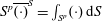 $S^{p}\overline{(\cdot )}^{S}=\int _{S^{p}}(\cdot )\,\text{d}S$
. Note that the term on the left-hand side of (3.6) involves the dipole contribution (
 $n=1$
) of the radial component of the incoming velocity; and this is directly related to the undisturbed density-weighted radial velocity averaged over the particle surface (right-hand side of (3.6)). Prior to discussing the term within the square brackets in (3.5), we remark on the following aspects of
 $\overline{\boldsymbol{w}_{1r}^{in}}^{S}$
. First, we note that since we are dealing with inviscid forces, the boundary condition to be satisfied at the particle surface is only the no-penetration boundary condition. For any complex incoming flow field that may be written as a summation of plane waves, the dipole component of the radial velocity of each plane wave needs to satisfy the no-penetration boundary condition. From the relation,
 $\boldsymbol{w}_{1r}^{in}=(\boldsymbol{w}_{1}^{in}\boldsymbol{\cdot }\boldsymbol{n})\boldsymbol{n}$
, it can be seen that the term
 $\overline{\boldsymbol{w}_{1r}^{in}}^{S}$
succinctly represents the radial velocity of the complex incoming flow that must be cancelled by the no-penetration condition. Secondly, as shown in appendix C, the following mathematical manipulation allows us to write the surface average in terms of volume average over the particle:
 $$\begin{eqnarray}\displaystyle \overline{\boldsymbol{w}_{1r}^{in}}^{S}=\overline{(\boldsymbol{w}_{1}^{in}\boldsymbol{\cdot }\boldsymbol{n})\boldsymbol{n}}^{S}={\textstyle \frac{1}{3}}\overline{\boldsymbol{w}_{1}^{in}}^{V}+{\textstyle \frac{1}{3}}\overline{\boldsymbol{r}\unicode[STIX]{x1D735}\boldsymbol{\cdot }\boldsymbol{w}_{1}^{in}}^{V}, & & \displaystyle\end{eqnarray}$$
where
 $\boldsymbol{r}$
is the radial vector from the centre of the sphere.
We now elaborate on the term within the square brackets in (3.5), which can be written as a ratio of two rational expressions as:
 $$\begin{eqnarray}\displaystyle {\displaystyle \frac{-1}{k_{inv}R}}{\displaystyle \frac{h_{1}^{(2)}(k_{inv}R)}{{h_{1}^{(2)}}^{\prime }(k_{inv}R)}}=\frac{1+\text{i}k_{inv}R}{1+(1+\text{i}k_{inv}R)^{2}}. & & \displaystyle\end{eqnarray}$$
It is best to express
 $k_{inv}R$
in terms of non-dimensional frequency for reasons which shall be discussed below. We begin by defining a non-dimensional frequency,
 $\tilde{s}=sR/c_{0}=\text{i}\unicode[STIX]{x1D714}R/c_{0}=\text{i}kR$
. Note that in the inviscid context,
 $\tilde{s}$
will be purely imaginary, as the wavenumber
 $k$
is real valued. Following Parmar et al. (Reference Parmar, Haselbacher and Balachandar2012), the expression in (3.8) is termed the inviscid-unsteady transfer function (
 $G_{iu}$
) and expressed as:
 $$\begin{eqnarray}\displaystyle G_{iu}=\frac{1+\tilde{s}}{1+(1+\tilde{s})^{2}}. & & \displaystyle\end{eqnarray}$$
Therefore (3.5) which is the inviscid-unsteady force (
 $\boldsymbol{F}_{iu}$
) in the frequency/Laplace space may be rewritten as:
 $$\begin{eqnarray}\displaystyle {\mathcal{L}}(\boldsymbol{F}_{iu})={\displaystyle \frac{4}{3}}\unicode[STIX]{x03C0}R^{3}\unicode[STIX]{x1D70C}_{ref}sG_{iu}\frac{\widehat{w_{1r}^{in}}}{\cos \unicode[STIX]{x1D703}}\boldsymbol{e}_{z}=4\unicode[STIX]{x03C0}R^{3}G_{iu}{\mathcal{L}}\left({\displaystyle \frac{\unicode[STIX]{x2202}}{\unicode[STIX]{x2202}t}}\overline{(\unicode[STIX]{x1D70C}\boldsymbol{u}_{r})^{un}}^{S}\right), & & \displaystyle\end{eqnarray}$$
where we have used the equivalence established in (3.6) and in addition
 $\unicode[STIX]{x1D70C}_{ref}\boldsymbol{w}_{1r}$
has been replaced with
 $\unicode[STIX]{x1D70C}\boldsymbol{u}_{r}$
. This is because (i) using (2.8)
 $\unicode[STIX]{x1D70C}_{ref}\boldsymbol{w}_{1r}=\unicode[STIX]{x1D70C}_{0}\boldsymbol{u}_{1r}$
and to linear approximation,
 $\unicode[STIX]{x1D70C}_{0}\boldsymbol{u}_{1r}$
may be replaced with
 $(\unicode[STIX]{x1D70C}_{0}+\unicode[STIX]{x1D70C}_{1}^{in})\boldsymbol{u}_{1r}$
and (ii)
 $(\unicode[STIX]{x1D70C}_{0}+\unicode[STIX]{x1D70C}_{1}^{in})\boldsymbol{u}_{1r}$
can be replaced with
 $(\unicode[STIX]{x1D70C}\boldsymbol{u}_{r})^{un}$
from (2.5). Here
 $\boldsymbol{u}_{r}=(\boldsymbol{u}\boldsymbol{\cdot }\boldsymbol{n})\boldsymbol{n}$
is the radial component of velocity. Laplace inverse of (3.10) leads to a convolution integral and we obtain the inviscid-unsteady force in the time domain as:
 $$\begin{eqnarray}\displaystyle \boldsymbol{F}_{iu}(t)=4\unicode[STIX]{x03C0}R^{3}\int _{\tilde{\unicode[STIX]{x1D709}}=-\infty }^{\tilde{t}}K_{iu}(\tilde{t}-\tilde{\unicode[STIX]{x1D709}})\left[\frac{\unicode[STIX]{x2202}}{\unicode[STIX]{x2202}t}\overline{(\unicode[STIX]{x1D70C}\boldsymbol{u}_{r})^{un}}^{S}\right]_{\tilde{t}=\tilde{\unicode[STIX]{x1D709}}}\,\text{d}\tilde{\unicode[STIX]{x1D709}}, & & \displaystyle\end{eqnarray}$$
where,
 $K_{iu}={\mathcal{L}}^{-1}(G_{iu})$
is the inviscid-unsteady kernel in the time domain (Longhorn Reference Longhorn1952) and
 ${\mathcal{L}}^{-1}$
denotes Laplace inverse. Specifically,
 $$\begin{eqnarray}\displaystyle K_{iu}(\tilde{t}-\tilde{\unicode[STIX]{x1D709}})=\text{e}^{-(\tilde{t}-\tilde{\unicode[STIX]{x1D709}})}\cos (\tilde{t}-\tilde{\unicode[STIX]{x1D709}}), & & \displaystyle\end{eqnarray}$$
where,
 $\tilde{t}=tc_{0}/R$
and
 $\tilde{\unicode[STIX]{x1D709}}=\unicode[STIX]{x1D709}c_{0}/R$
are non-dimensional times. The ambient speed of sound (
 $c_{0}$
) and particle radius (
 $R$
) are used as the velocity and length scales, respectively. We observe that (3.11) naturally splits into a space (surface average) component and time (kernel) component. Therefore we argue that it is natural to replace the terms involving
 $k_{inv}R$
with non-dimensional frequency (
 $-\text{i}\tilde{s}$
) in the force expression in (3.5). Nevertheless it is important to note that this replacement was carried out only to that portion of the force expression not concerning surface averages.
We began the analysis for a single incident travelling acoustic wave of frequency,
 $\unicode[STIX]{x1D714}$
and as a result the left-hand side of (3.6) is a function of
 $k_{inv}$
and
 $\unicode[STIX]{x1D714}$
, since
 $\widehat{w_{1r}^{in}}$
depends on
 $k_{inv}$
,
 $\unicode[STIX]{x1D714}$
and particle size,
 $R$
, as can be seen from (A 3); and dependent on the details of the incident wave. On the other hand, by transforming to the right-hand side of (3.6), the same quantity is now expressed as the Laplace transform of the average of the radial component of the incident wave velocity over the surface of the particle. This equivalence is the key step in obtaining the Faxén’s force (for unsteady viscous compressible flows) by accounting for ambient flow non-uniformity in terms of the surface (or volume) average of the incident flow.
In the case of a complex compressible flow over a stationary spherical particle, this oncoming flow can be expressed as a superposition of waves of varying frequency and orientation. In the linear limit, the inviscid-unsteady force that arises from each of these waves can be independently calculated and superposed to obtain the overall inviscid-unsteady force. The remarkable feature of Faxén’s form of the force, given in (3.6), is that it remains unchanged during superposition. This is due to the fact that superposition commutes with the Laplace transform, time derivative and the surface average. Thus, the inviscid-unsteady force due to a complex oncoming flow can be readily obtained by interpreting
 $\overline{\boldsymbol{w}_{1r}^{in}(\boldsymbol{r},t)}^{S}$
to be the surface average of the complex density-weighted radial velocity over the particle. Such a convenient representation of superposition is not possible if the inviscid-unsteady were to be written in the non-Faxén form (i.e. in terms of the left-hand side of (3.6)).
Therefore the total inviscid force acting on a finite-sized spherical particle located in an inhomogeneous compressible medium is obtained by summing (3.3) and (3.11) as:
 $$\begin{eqnarray}\displaystyle \boldsymbol{F}_{inv}(t) & = & \displaystyle \boldsymbol{F}_{un}(t)+\boldsymbol{F}_{iu}(t)={\displaystyle \frac{4}{3}}\unicode[STIX]{x03C0}R^{3}\overline{\unicode[STIX]{x1D70C}^{un}\frac{\text{D}\boldsymbol{u}}{\text{D}t}^{un}}^{V}\nonumber\\ \displaystyle & & \displaystyle +\,4\unicode[STIX]{x03C0}R^{3}\int _{\tilde{\unicode[STIX]{x1D709}}=-\infty }^{\tilde{t}}K_{iu}(\tilde{t}-\tilde{\unicode[STIX]{x1D709}})\left[\frac{\unicode[STIX]{x2202}}{\unicode[STIX]{x2202}t}\overline{(\unicode[STIX]{x1D70C}\boldsymbol{u}_{r})^{un}}^{S}\right]_{\tilde{t}=\tilde{\unicode[STIX]{x1D709}}}\,\text{d}\tilde{\unicode[STIX]{x1D709}}.\end{eqnarray}$$
In the above equation, the expression for the inviscid-unsteady force assumes a stationary particle and ignores nonlinear effects, but no such restriction applies for the undisturbed force.
3.2.2 Viscous forces
In (3.6), we established how the radial velocity component may be written in terms of the surface average of the incoming density-weighted velocity and thereby obtained the Faxén form of the inviscid force in the time domain. Similarly the tangential velocity may be written in terms of the volume average of the incoming density-weighted velocity as:
 $$\begin{eqnarray}\displaystyle -{\displaystyle \frac{4}{3}}\unicode[STIX]{x03C0}R^{3}\unicode[STIX]{x1D70C}_{ref}(\text{i}\unicode[STIX]{x1D714})\left[\frac{\widehat{w_{1\unicode[STIX]{x1D703}}^{in}}}{\sin \unicode[STIX]{x1D703}}\right]\boldsymbol{e}_{z}={\displaystyle \frac{4}{3}}\unicode[STIX]{x03C0}R^{3}\unicode[STIX]{x1D70C}_{ref}{\mathcal{L}}\left({\displaystyle \frac{\unicode[STIX]{x2202}}{\unicode[STIX]{x2202}t}}\overline{\boldsymbol{w}_{1}^{in}(\boldsymbol{r},t)}^{V}\right). & & \displaystyle\end{eqnarray}$$
In order to express the viscous forces in the time domain, we shall write the force expression in Laplace space using surface average of the normal and total velocities. It can be seen from appendix D that:
 $$\begin{eqnarray}\displaystyle \overline{\boldsymbol{w}_{1}^{in}}^{V}={\textstyle \frac{3}{2}}\overline{\boldsymbol{w}_{1}^{in}}^{S}-{\textstyle \frac{3}{2}}\overline{(\boldsymbol{w}_{1}^{in}\boldsymbol{\cdot }\boldsymbol{n})\boldsymbol{n}}^{S}. & & \displaystyle\end{eqnarray}$$
It must be mentioned that the equivalences established in (3.7) and (3.15) have been proven by considering a single frequency acoustic wave propagating over the particle. Due to the linear nature of the relation it remains applicable to any field that can be represented as a linear superposition of such waves. Substituting (3.6), (3.14) and (3.15) in (3.1), the force due to the disturbance flow may be written as:
 $$\begin{eqnarray}\displaystyle {\mathcal{L}}(\boldsymbol{F}_{d})={\displaystyle \frac{4}{3}}\unicode[STIX]{x03C0}R^{3}\unicode[STIX]{x1D70C}_{ref}\left[3G^{V}{\mathcal{L}}\left({\displaystyle \frac{\unicode[STIX]{x2202}}{\unicode[STIX]{x2202}t}}\overline{(\boldsymbol{w}_{1}^{in}(\boldsymbol{r},t)\boldsymbol{\cdot }\boldsymbol{n})\boldsymbol{n}}^{S}\right)+G^{S}{\mathcal{L}}\left({\displaystyle \frac{\unicode[STIX]{x2202}}{\unicode[STIX]{x2202}t}}\overline{\boldsymbol{w}_{1}^{in}(\boldsymbol{r},t)}^{S}\right)\right], & & \displaystyle\end{eqnarray}$$
where,
 $$\begin{eqnarray}\displaystyle \left.\begin{array}{@{}c@{}}\displaystyle G^{V}={\displaystyle \frac{1-\left[\displaystyle {\displaystyle \frac{h_{1}^{(2)}(kR)}{kR{h_{1}^{(2)}}^{\prime }(kR)}}\left(1-\displaystyle {\displaystyle \frac{k_{\unicode[STIX]{x1D708}}Rh_{2}^{(2)}(k_{\unicode[STIX]{x1D708}}R)}{h_{1}^{(2)}(k_{\unicode[STIX]{x1D708}}R)}}\right)\right]}{2-{\displaystyle \frac{k_{\unicode[STIX]{x1D708}}Rh_{2}^{(2)}(k_{\unicode[STIX]{x1D708}}R)}{h_{1}^{(2)}(k_{\unicode[STIX]{x1D708}}R)}}-{\displaystyle \frac{2h_{1}^{(2)}(kR)}{kR{h_{1}^{(2)}}^{\prime }(kR)}}}};\\ \displaystyle G^{S}={\displaystyle \frac{-3\left(1\displaystyle -{\displaystyle \frac{h_{1}^{(2)}(kR)}{kR{h_{1}^{(2)}}^{\prime }(kR)}}\right)}{2-\displaystyle {\displaystyle \frac{k_{\unicode[STIX]{x1D708}}Rh_{2}^{(2)}(k_{\unicode[STIX]{x1D708}}R)}{h_{1}^{(2)}(k_{\unicode[STIX]{x1D708}}R)}}-{\displaystyle \frac{2h_{1}^{(2)}(kR)}{kR{h_{1}^{(2)}}^{\prime }(kR)}}}}.\end{array}\right\} & & \displaystyle\end{eqnarray}$$
Note that
 $kR$
and
 $k_{\unicode[STIX]{x1D708}}R$
in (3.17) may be written in terms of the Laplace variable as
 $-\text{i}sR/c_{0}$
and
 $-\text{i}\sqrt{sR^{2}/\unicode[STIX]{x1D708}}$
, respectively. Now taking the Laplace inverse of (3.16), we obtain the Faxén form of the disturbed force (
 $\boldsymbol{F}^{d}$
) in the time domain as:
 $$\begin{eqnarray}\displaystyle \boldsymbol{F}_{d}(t) & = & \displaystyle 6R\unicode[STIX]{x03C0}\unicode[STIX]{x1D708}\overline{(\unicode[STIX]{x1D70C}\boldsymbol{u})^{un}}^{S}+4\unicode[STIX]{x03C0}R^{3}\int _{\tilde{\unicode[STIX]{x1D709}}=-\infty }^{\tilde{t}}K_{iu}(\tilde{t}-\tilde{\unicode[STIX]{x1D709}})\left[\frac{\unicode[STIX]{x2202}}{\unicode[STIX]{x2202}t}\overline{(\unicode[STIX]{x1D70C}\boldsymbol{u}_{r})^{un}}^{S}\right]_{\tilde{t}=\tilde{\unicode[STIX]{x1D709}}}\,\text{d}\tilde{\unicode[STIX]{x1D709}}\nonumber\\ \displaystyle & & \displaystyle +\,18R^{2}\sqrt{\unicode[STIX]{x03C0}\unicode[STIX]{x1D708}}\left.\int _{\unicode[STIX]{x1D709}=-\infty }^{t}K_{vu}^{V}(t-\unicode[STIX]{x1D709})\frac{\unicode[STIX]{x2202}}{\unicode[STIX]{x2202}t}\overline{(\unicode[STIX]{x1D70C}\boldsymbol{u}_{r})^{un}}^{S}\right|_{t=\unicode[STIX]{x1D709}}\,\text{d}\unicode[STIX]{x1D709}\nonumber\\ \displaystyle & & \displaystyle +\,6R^{2}\sqrt{\unicode[STIX]{x03C0}\unicode[STIX]{x1D708}}\left.\int _{\unicode[STIX]{x1D709}=-\infty }^{t}K_{vu}^{S}(t-\unicode[STIX]{x1D709})\frac{\unicode[STIX]{x2202}}{\unicode[STIX]{x2202}t}\overline{(\unicode[STIX]{x1D70C}\boldsymbol{u})^{un}}^{S}\right|_{t=\unicode[STIX]{x1D709}}\,\text{d}\unicode[STIX]{x1D709}.\end{eqnarray}$$
The above equation (3.18), to linear approximation, is an exact expression for the disturbance force in the time domain acting on an stationary spherical particle in a viscous compressible medium subjected to an inhomogeneous ambient flow. In obtaining the above expression, we separate the transfer functions as:
 $$\begin{eqnarray}\displaystyle G^{V}=G_{iu}+G_{vu}^{V}\quad \text{and}\quad G^{S}=G_{qs}+G_{vu}^{S}, & & \displaystyle\end{eqnarray}$$
where the transfer function
 $G^{V}$
is split into an inviscid component and a viscous component. While
 $G_{iu}$
accounts for the inviscid-unsteady force which was discussed earlier,
 $G_{vu}^{V}$
is new and arises only in the context of viscous compressible flows. Further,
 $G^{S}$
has been separated into
 $G_{qs}$
and
 $G_{vu}^{S}$
and both terms lead to viscous forces. On Laplace inverse, the above four transfer functions may be written in the time domain as:
 $$\begin{eqnarray}\displaystyle \left.\begin{array}{@{}c@{}}\displaystyle {\mathcal{L}}^{-1}(G_{iu})={\displaystyle \frac{c_{0}}{R}}K_{iu},\\ \displaystyle {\mathcal{L}}^{-1}(G_{vu}^{V})={\displaystyle \frac{9}{2R}}\sqrt{{\displaystyle \frac{\unicode[STIX]{x1D708}}{\unicode[STIX]{x03C0}}}}K_{vu}^{V},\\ \displaystyle {\mathcal{L}}^{-1}(G_{vu}^{S})={\displaystyle \frac{9}{2R}}\sqrt{{\displaystyle \frac{\unicode[STIX]{x1D708}}{\unicode[STIX]{x03C0}}}}K_{vu}^{S},\\ \displaystyle G_{qs}={\displaystyle \frac{9\unicode[STIX]{x1D708}}{2sR^{2}}}.\end{array}\right\} & & \displaystyle\end{eqnarray}$$
Therefore the total force (
 $\boldsymbol{F}$
), which is the sum of undisturbed (
 $\boldsymbol{F}_{un}$
) and disturbed force (
 $\boldsymbol{F}_{d}$
), is given by:
 $$\begin{eqnarray}\displaystyle \boldsymbol{F}(t) & = & \displaystyle {\displaystyle \frac{4}{3}}\unicode[STIX]{x03C0}R^{3}\overline{\unicode[STIX]{x1D70C}^{un}\frac{\text{D}\boldsymbol{u}}{\text{D}t}^{un}}^{V}+6R\unicode[STIX]{x03C0}\unicode[STIX]{x1D708}\overline{(\unicode[STIX]{x1D70C}\boldsymbol{u})^{un}}^{S}+4\unicode[STIX]{x03C0}R^{3}\int _{\tilde{\unicode[STIX]{x1D709}}=-\infty }^{\tilde{t}}K_{iu}(\tilde{t}-\tilde{\unicode[STIX]{x1D709}})\left[\frac{\unicode[STIX]{x2202}}{\unicode[STIX]{x2202}t}\overline{(\unicode[STIX]{x1D70C}\boldsymbol{u}_{r})^{un}}^{S}\right]_{\tilde{t}=\tilde{\unicode[STIX]{x1D709}}}\,\text{d}\tilde{\unicode[STIX]{x1D709}}\nonumber\\ \displaystyle & & \displaystyle +\,18R^{2}\sqrt{\unicode[STIX]{x03C0}\unicode[STIX]{x1D708}}\left.\int _{\unicode[STIX]{x1D709}=-\infty }^{t}K_{vu}^{V}(t-\unicode[STIX]{x1D709})\frac{\unicode[STIX]{x2202}}{\unicode[STIX]{x2202}t}\overline{(\unicode[STIX]{x1D70C}\boldsymbol{u}_{r})^{un}}^{S}\right|_{t=\unicode[STIX]{x1D709}}\,\text{d}\unicode[STIX]{x1D709}\nonumber\\ \displaystyle & & \displaystyle +\,6R^{2}\sqrt{\unicode[STIX]{x03C0}\unicode[STIX]{x1D708}}\left.\int _{\unicode[STIX]{x1D709}=-\infty }^{t}K_{vu}^{S}(t-\unicode[STIX]{x1D709})\frac{\unicode[STIX]{x2202}}{\unicode[STIX]{x2202}t}\overline{(\unicode[STIX]{x1D70C}\boldsymbol{u})^{un}}^{S}\right|_{t=\unicode[STIX]{x1D709}}\,\text{d}\unicode[STIX]{x1D709}.\end{eqnarray}$$
In summary, the first term in (3.21) is the force due to the stress field of the undisturbed ambient flow on the volume of the gas/fluid occupied by the particle if the particle were absent. The rest of the forces originate from the disturbance field due to the particle. The second term is the quasi-steady drag experienced by the particle and arises from the quasi-steady transfer function,
 $G_{qs}$
. This is indeed Faxén’s law described in Faxén (Reference Faxén1922). The third term is the inviscid history force due to the transfer function,
 $G_{iu}$
as described in § 3.2.1. The fourth and fifth terms are viscous history forces originating from
 $G_{vu}^{S}$
and
 $G_{vu}$
respectively. While the fourth term is new and arises only in viscous compressible flows, the last term is the well known viscous-unsteady force (also known as Basset history force), however now expressed in terms of appropriate surface averages. It should be mentioned that since the undisturbed force acts on the volume of the fluid occupied by the particle, it is expressed as a volume-averaged density-weighted velocity. All other force components occur because of the presence of the particle and are due to the creation of the disturbance field by demanding that the normal and tangential velocities on the particle surface are zero. Therefore the quasi-steady, inviscid-unsteady and viscous-unsteady forces are expressed as surface-averaged density-weighted velocities. Moreover, the inviscid forces have been written in terms of surface-averaged radial velocities since satisfying the no-penetration boundary condition would suffice for inviscid flows. However for viscous flows one also needs to satisfy the no-slip boundary condition (in addition to no-penetration) at the particle interface; and as a consequence the viscous force components involve the surface average of the velocity vector in its entirety in addition to the radial component.
Parmar et al. (Reference Parmar, Haselbacher and Balachandar2012) also presented a similar force expression, however their analysis was restricted to the limit where the particle radius is much smaller than the length scale of the ambient flow variation. Note that one needs to replace the surface average of the normal velocity in the second and third terms of (3.21) with the corresponding volume average using (3.7) to compare against the works in Zwanzig & Bixon (Reference Zwanzig and Bixon1970), Parmar et al. (Reference Parmar, Haselbacher and Balachandar2012). Furthermore, based on scaling arguments, they ignored terms involving
 $\overline{\boldsymbol{r}\unicode[STIX]{x1D735}\boldsymbol{\cdot }\boldsymbol{w}_{1}^{in}}^{V}$
in (3.7) which can be justified only in the limit of
 $R\ll \unicode[STIX]{x1D706}$
. The present derivation is rigorous and places no restriction on the particle size compared to the length scale of the incoming flow variation. The only limitation is that the present linear formulation is restricted to negligible Reynolds and Mach numbers.
The history kernels in the frequency domain (i.e.
 $G_{iu},G_{vu}^{V}$
and
 $G_{vu}^{S}$
) are explicitly known. However, in order to compute the force in the time domain, as given in the above equation, the history kernels (i.e.
 $K_{iu},K_{vu}^{V}$
and
 $K_{vu}^{S}$
) are needed in the time domain. While analytic expression for
 $K_{iu}$
exists, explicit expressions for
 $K_{vu}^{V}$
and
 $K_{vu}^{S}$
are not available.
4 Faxén form of force for nonlinear flows
The discussion so far was limited to flows where the convective terms could be neglected (e.g. interaction of a weak shock/acoustic wave with a particle) as the equations solved were the linearized Navier–Stokes equations. For example, if we consider a stationary particle situated in a flow that is both steady and inviscid, one obtains from (3.13) the force on the particle to be:
 $$\begin{eqnarray}\displaystyle {\textstyle \frac{4}{3}}\unicode[STIX]{x03C0}R^{3}\overline{(\unicode[STIX]{x1D70C}\boldsymbol{u})^{un}\boldsymbol{\cdot }\unicode[STIX]{x1D735}\boldsymbol{u}^{un}}^{V}. & & \displaystyle\end{eqnarray}$$
This contribution is entirely due to the undisturbed ambient flow and the contribution from the disturbance flow is identically zero according to (3.13). However, if one were to consider a steady converging or diverging flow over a sphere, the particle does experience a significant non-zero added-mass force as described in the pioneering work of Taylor (Reference Taylor1928). This added-mass force is due to the convective acceleration of the ambient fluid as seen by the particle, as opposed to the temporal acceleration of the ambient fluid. This additional contribution to the force can be evaluated in the following way. For the case of a stationary particle considered here, the impulse on the fluid surrounding the particle can be expressed as (Landau & Lifschitz Reference Landau and Lifschitz1987; Lamb Reference Lamb1993; Ohl, Tijink & Prosperetti Reference Ohl, Tijink and Prosperetti2003):
 $$\begin{eqnarray}\displaystyle \boldsymbol{P}={\textstyle \frac{4}{3}}\unicode[STIX]{x03C0}R^{3}C_{M}(\unicode[STIX]{x1D70C}\boldsymbol{u})^{un}, & & \displaystyle\end{eqnarray}$$
where the added-mass coefficient
 $C_{M}$
for a sphere is
 $1/2$
. As argued by Taylor (Reference Taylor1928), even in a steady flow, the spatial variation in the ambient flow will give rise to spatial variation in the impulse and an attendant added-mass force of the form:
 $$\begin{eqnarray}\displaystyle \boldsymbol{u}^{un}\boldsymbol{\cdot }\unicode[STIX]{x1D735}\boldsymbol{P}={\textstyle \frac{4}{3}}\unicode[STIX]{x03C0}R^{3}C_{M}\boldsymbol{u}^{un}\boldsymbol{\cdot }\unicode[STIX]{x1D735}(\unicode[STIX]{x1D70C}\boldsymbol{u})^{un}. & & \displaystyle\end{eqnarray}$$
The above force is due to convective acceleration of the fluid. It is clearly nonlinear in velocity and as a result does not arise in the force expression derived from the linearized Navier–Stokes equations and is not included in (3.21). In order to interpret this force, we will also consider the corresponding force due to temporal acceleration which is given by:
 $$\begin{eqnarray}\displaystyle {\displaystyle \frac{\unicode[STIX]{x2202}\boldsymbol{P}}{\unicode[STIX]{x2202}t}}={\displaystyle \frac{4}{3}}\unicode[STIX]{x03C0}R^{3}C_{M}{\displaystyle \frac{\unicode[STIX]{x2202}}{\unicode[STIX]{x2202}t}}(\unicode[STIX]{x1D70C}\boldsymbol{u})^{un}. & & \displaystyle\end{eqnarray}$$
The above can be combined with (4.3) and rewritten as:
 $$\begin{eqnarray}\displaystyle \frac{4}{3}\unicode[STIX]{x03C0}R^{3}C_{M}\unicode[STIX]{x1D70C}^{un}\frac{\text{D}\boldsymbol{u}^{un}}{\text{D}t}+\frac{4}{3}\unicode[STIX]{x03C0}R^{3}C_{M}\boldsymbol{u}^{un}\frac{\text{D}\unicode[STIX]{x1D70C}^{un}}{\text{D}t}. & & \displaystyle\end{eqnarray}$$
The first term is the familiar added-mass force due to acceleration of the undisturbed ambient flow in a constant-density incompressible medium (Maxey & Riley Reference Maxey and Riley1983). The second added-mass force term arises when there is density variation in the direction of motion of the undisturbed ambient flow. Such an additional force has been recognized in the context of particle motion in a density stratified flow (Eames & Hunt Reference Eames and Hunt1997). The above inviscid-unsteady force is also in agreement with the expression derived by Eames & Hunt (Reference Eames and Hunt2004) for the force on a sphere moving unsteadily in a homogeneous compressed flow. Also, it has been computationally verified through finite Reynolds number simulations that the above expressions for the inviscid added-mass force remain unaffected even in a viscous flow (Bagchi & Balachandar Reference Bagchi and Balachandar2002). However, there will also be viscous contributions arising from the convective acceleration.
The above formulation does not account for the compressibility of the ambient undisturbed flow or the perturbation flow generated by the particle. Furthermore, it is assumed that the particle is much smaller than the length scale on which the undisturbed ambient flow varies. Because of this later assumption, terms such as
 $\boldsymbol{u}^{un}$
and
 $\text{D}\boldsymbol{u}^{un}/\text{D}t$
are considered to be evaluated at the particle centre and there is no need to average these quantities over the surface or volume of the particle. For the present purposes, we need to both account for flow compressibility and relax the requirement that the particle be much smaller than the ambient flow scales. Since a rigorous derivation of the nonlinear effects under these more complex conditions is lacking, here we generalize (4.3) as:
 $$\begin{eqnarray}\displaystyle \frac{4}{3}\unicode[STIX]{x03C0}R^{3}\int _{\tilde{\unicode[STIX]{x1D709}}=-\infty }^{\tilde{t}}K_{iu}(\tilde{t}-\tilde{\unicode[STIX]{x1D709}})\overline{\boldsymbol{u}^{un}}^{V}\boldsymbol{\cdot }\unicode[STIX]{x1D735}\overline{(\unicode[STIX]{x1D70C}\boldsymbol{u})^{un}}^{S}\,\text{d}\tilde{\unicode[STIX]{x1D709}}. & & \displaystyle\end{eqnarray}$$
The above nonlinear contribution to the inviscid-unsteady force arising from the past history of convective acceleration can be added to the inviscid-unsteady force arising from temporal acceleration in (3.11). For the viscous-unsteady force however, the correct means of accounting for convective acceleration is still under question. Therefore, in accordance with the earlier works of Maxey & Riley (Reference Maxey and Riley1983) and Magnaudet & Eames (Reference Magnaudet and Eames2000), we will use the time derivative following the particle,
 $\text{d}/\text{d}t$
, in the acceleration term corresponding to the viscous history force. The resulting nonlinear Faxén form of the force can thus be expressed as:
 $$\begin{eqnarray}\displaystyle \boldsymbol{F}^{GF}(t) & = & \displaystyle {\displaystyle \frac{4}{3}}\unicode[STIX]{x03C0}R^{3}\overline{\unicode[STIX]{x1D70C}^{un}\frac{\text{D}\boldsymbol{u}}{\text{D}t}^{un}}^{V}+6R\unicode[STIX]{x03C0}\unicode[STIX]{x1D708}\overline{(\unicode[STIX]{x1D70C}\boldsymbol{u})^{un}}^{S}\unicode[STIX]{x1D6F7}(Re,M)\nonumber\\ \displaystyle & & \displaystyle +\,4\unicode[STIX]{x03C0}R^{3}\int _{\tilde{\unicode[STIX]{x1D709}}=-\infty }^{\tilde{t}}K_{iu}(\tilde{t}-\tilde{\unicode[STIX]{x1D709}};M)\left[\overline{{\displaystyle \frac{\text{D}}{\text{D}t}}}\overline{(\unicode[STIX]{x1D70C}\boldsymbol{u}_{r})^{un}}^{S}\right]_{\tilde{t}=\tilde{\unicode[STIX]{x1D709}}}\,\text{d}\tilde{\unicode[STIX]{x1D709}}\nonumber\\ \displaystyle & & \displaystyle +\,18R^{2}\sqrt{\unicode[STIX]{x03C0}\unicode[STIX]{x1D708}}\left.\int _{\unicode[STIX]{x1D709}=-\infty }^{t}K_{vu}^{V}(t-\unicode[STIX]{x1D709};Re,M){\displaystyle \frac{\text{d}}{\text{d}t}}\overline{(\unicode[STIX]{x1D70C}\boldsymbol{u}_{r})^{un}}^{S}\right|_{t=\unicode[STIX]{x1D709}}\,\text{d}\unicode[STIX]{x1D709}\nonumber\\ \displaystyle & & \displaystyle +\,6R^{2}\sqrt{\unicode[STIX]{x03C0}\unicode[STIX]{x1D708}}\left.\int _{\unicode[STIX]{x1D709}=-\infty }^{t}K_{vu}^{S}(t-\unicode[STIX]{x1D709};Re,M)\,{\displaystyle \frac{\text{d}}{\text{d}t}}\overline{(\unicode[STIX]{x1D70C}\boldsymbol{u})^{un}}^{S}\right|_{t=\unicode[STIX]{x1D709}}\,\text{d}\unicode[STIX]{x1D709},\end{eqnarray}$$
where,
 $\overline{\text{D}}/\text{D}t=\unicode[STIX]{x2202}/\unicode[STIX]{x2202}t+\overline{\boldsymbol{u}^{un}}^{V}\boldsymbol{\cdot }\unicode[STIX]{x1D735}$
and the superscript
 $GF$
indicates generalized Faxén form. There are other effects of nonlinearity as well. In particular, the linearized Navier–Stokes equations considered in (2.6) and (2.7) require the particle Reynolds number and Mach number to be very small. The Reynolds and Mach numbers are based on the undisturbed fluid velocity and can be defined as:
 $$\begin{eqnarray}\displaystyle Re={\displaystyle \frac{2R\overline{|\boldsymbol{u}^{un}|}^{V}}{\unicode[STIX]{x1D708}}}\quad \text{and}\quad M={\displaystyle \frac{\overline{|\boldsymbol{u}^{un}|}^{V}}{\overline{c^{un}}^{V}}}, & & \displaystyle\end{eqnarray}$$
where
 $\overline{\unicode[STIX]{x1D707}}^{V}$
is the viscosity and
 $\overline{c^{\text{un}}}^{V}$
is the speed of sound of the undisturbed ambient flow averaged over the volume where the particle is located and
 $|\boldsymbol{u}^{un}|$
denotes the magnitude of
 $\boldsymbol{u}^{un}$
. It is important to note the following with regards to (4.7):
-
(i) Nonlinear effects show up in quasi-steady drag (represented by the second term on the right-hand side of (4.7)) via the finite Reynolds and Mach number correction factor,
 $\unicode[STIX]{x1D6F7}$
(Clift & Gauvin Reference Clift and Gauvin1970; Crowe, Sommerfeld & Tsuji Reference Crowe, Sommerfeld and Tsuji1998; Loth Reference Loth2008; Parmar, Haselbacher & Balachandar Reference Parmar, Haselbacher and Balachandar2010).
$\unicode[STIX]{x1D6F7}$
reduces to unity in the linear limit of
$Re\rightarrow 0$
and
$M\rightarrow 0$
.
-
(ii) Nonlinear effects in the inviscid-unsteady force are included by replacing
$\unicode[STIX]{x2202}/\unicode[STIX]{x2202}t$
terms in (3.21) with the substantial derivative
$\overline{\text{D}}/\text{D}t$
in (4.7), which includes the nonlinear convective acceleration. -
(iii) The inviscid kernel
$K_{iu}$
, as expressed in (3.12), is valid in the limit of zero Mach number. The behaviour of the kernel at finite Mach numbers has been discussed in the work of Parmar, Haselbacher & Balachandar (Reference Parmar, Haselbacher and Balachandar2008). -
(iv) In the viscous-unsteady force,
$\unicode[STIX]{x2202}/\unicode[STIX]{x2202}t$
is replaced with
$\text{d}/\text{d}t$
. These replacements of
$\unicode[STIX]{x2202}/\unicode[STIX]{x2202}t$
with either
$\text{D}/\text{D}t$
or
$\text{d}/\text{d}t$
are by no means unique or rigorous. Here we follow the work of Maxey & Riley (Reference Maxey and Riley1983) and its finite Reynolds number extensions as suggested by Magnaudet & Eames (Reference Magnaudet and Eames2000). -
(v) The viscous kernels
$K_{vu}^{V}$
and
$K_{vu}^{S}$
are also functions of
$Re$
and
$M$
. Unfortunately, we have very little information or understanding of the viscous kernels even in the incompressible limit while their dependence on Reynolds number can be found in the works of Mei & Adrian (Reference Mei and Adrian1992), Michaelides (Reference Michaelides1992), Lovalenti & Brady (Reference Lovalenti and Brady1993a
,Reference Lovalenti and Brady
b
) and Kim, Elgobashi & Sirignano (Reference Kim, Elgobashi and Sirignano1998). -
(vi) In the linear limit,
$\overline{\text{D}}/\text{D}t$
reduces to
$\unicode[STIX]{x2202}/\unicode[STIX]{x2202}t$
, the coefficient
$\unicode[STIX]{x1D6F7}$
takes the value of unity and the kernels take their corresponding limiting values as shown in (3.20); thereby, (4.7) reduces to (3.21).


5 Summary: Faxén form of the force and the corresponding limiting cases
In the inviscid limit, the nonlinear Faxén form of the force reduces to:
 $$\begin{eqnarray}\displaystyle \boldsymbol{F}_{inv}^{GF}(t)={\displaystyle \frac{4}{3}}\unicode[STIX]{x03C0}R^{3}\overline{\unicode[STIX]{x1D70C}^{un}\frac{\text{D}\boldsymbol{u}}{\text{D}t}^{un}}^{V}+4\unicode[STIX]{x03C0}R^{3}\int _{\tilde{\unicode[STIX]{x1D709}}=-\infty }^{\tilde{t}}K_{iu}(\tilde{t}-\tilde{\unicode[STIX]{x1D709}};M)\left[\overline{{\displaystyle \frac{\text{D}}{\text{D}t}}}\overline{(\unicode[STIX]{x1D70C}\boldsymbol{u}_{r})^{un}}^{S}\right]_{\tilde{t}=\tilde{\unicode[STIX]{x1D709}}}\,\text{d}\tilde{\unicode[STIX]{x1D709}}. & & \displaystyle\end{eqnarray}$$
The above equation (5.1) will be used in § 6 to predict the force on a fixed sphere subjected to an expansion fan when nonlinear effects are important. The other limiting cases are detailed in appendix E.
In summary, we began our analysis with a plane acoustic wave of a given frequency to impinge on a finite-sized stationary particle and obtained the force in the frequency domain. While the force expression in the frequency domain is known (Bedeaux & Mazur Reference Bedeaux and Mazur1974; Guz Reference Guz2009), we have expressed the force in a fashion that (i) allows explicit transformation to the time domain, and (ii) accounts for inhomogeneous ambient flows with no restriction on the length scale of variation. In other words, the current formulation clearly partitions the history forces (inviscid-unsteady and viscous-unsteady) into two components – one arising due to spatial variation in the ambient flow and another coming from unsteadiness of the flow. While the former leads to Faxén-like volume and surface averages to account for the spatial variation of the ambient flow, the latter leads to history kernels. In the context of homogeneous ambient flows, the spatial averages drop out while the history integrals of the unsteady components remain unchanged. The steady force is identical to Faxén’s correction expressed in terms of the surface average. Therefore the current formulation in essence is a generalization of Faxén’s theorem to viscous, unsteady and compressible flows as it fully accounts for arbitrary spatial variation of the incoming flow.
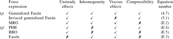
Table 1 concisely presents the various force forms discussed in this paper beginning with the Faxén form of the force (for unsteady viscous compressible flows) with nonlinear effects included and their simplifications under various limiting conditions such as (i) the inviscid limit, (ii) the incompressible limit (iii) the steady limit and (iv) the scenario when the particle size is much smaller than the length scale of the incoming flow. The table also lists the presence and/or absence of various physical effects such as unsteadiness, inhomogeneity, viscosity and compressibility in each of the force expressions. Depending on the problem of interest, and after analysing which of the above mentioned physical effects are important, the reader may accordingly choose one form over the other. The corresponding equation number of the resulting simplified (limited) force expression is also given.
Summary of the Faxén force with unsteady, viscous, compressible and non-homogeneous effects included; and its various limiting forms. The symbols
 ${\checkmark}$
and ✗ denote respectively the inclusion and exclusion of the given effects/physics in the corresponding force expression.

6 Application: drag on a finite-sized sphere due to interaction with an expansion fan
In this study we test our Faxén’s form of the force by applying it to compute the force experienced by an isolated spherical particle subjected to a planar expansion fan. For this purpose, we consider the flow over a sphere in a planar shock tube. We analyse two cases: (i) a weak expansion fan generated due to an initial pressure ratio of 1.05 and (ii) a strong expansion fan (initial pressure ratio = 2.5). We conduct highly resolved axisymmetric direct numerical simulations (DNS) where the compressible Euler equations are solved using the finite-volume methodology. In the simulations described, the fluxes are computed using a second-order accurate Roe scheme (Roe Reference Roe1981). The gradients are modified using a weighted essentially non-oscillatory (WENO) reconstruction technique (Haselbacher Reference Haselbacher2005). A fourth-order accurate Runge–Kutta scheme is used for time integration. The model is then compared against DNS results.
In both cases mentioned above, the particle centre is located
 $2.5$
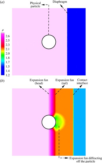
radii away from the initial diaphragm location and the simulation is conducted until the tail of the expansion fan completely crosses the particle. The diaphragm location was chosen such that the various flow discontinuities (shock, expansion fan and contact interface) clearly separate out before the head of expansion fan reaches the particle. Figure 1 shows the shock tube configuration for the second case (pressure ratio = 2.5) at (i) time,
 $t=0$
ms, before bursting of the diaphragm and (ii) at
 $t=0.3$
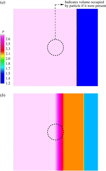
ms, as the expansion fan interacts with the particle. As can be seen in figure 1(b), the flow is extremely complex close to the particle, due to interaction of the incoming expansion fan and its diffraction around the particle. The finite-volume code/numerical simulation takes into account the details of this complex flow field to compute the force experienced by the particle. In contrast, the current Faxén’s force model requires only the ‘undisturbed’ flow properties averaged over the particle volume/surface. In other words, one simply needs to average the density/velocity over the volume that is occupied by the particle, in the absence of the particle. Therefore shown in figure 2 is the one-dimensional shock tube without the particle. In both figure 2(a)
 $(t=0~\text{ms})$
and figure 2(b)
 $(t=0.3~\text{ms})$
, the dashed circle represents the volume occupied by the actual particle in our simulations. Since we are interested in the undisturbed flow properties, we only need to focus on quantities within this imaginary sphere to compute the volume or surface-averaged quantities of interest (also see figure 3
a,b). In this specific case, since we are considering a one-dimensional planar shock tube, the necessary flow properties are analytically obtained (Liepmann & Roshko Reference Liepmann and Roshko1957) and substituted in (4.7) to obtain the force.
Total flow-field (undisturbed and disturbed effects inclusive) due to a one-dimensional planar shock tube with an initial pressure ratio of
 $2.5$
at times (a)
 $t=0~\text{ms}$
and (b)
 $t=0.3~\text{ms}$
, where one observes the diffraction of waves from the particle surface.

The ‘undisturbed’ one-dimensional planar shock tube with an initial pressure ratio of
 $2.5$
in the absence of the particle at times (a)
 $t=0~\text{ms}$
and (b)
 $t=0.3~\text{ms}$
. In both cases, the volume enclosed by the dashed circle represents the location of the particle in the DNS.

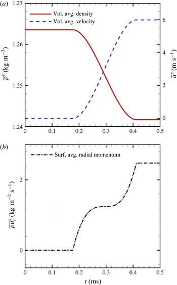
(a) Undisturbed density averaged over the particle with a diameter of 80 mm and (b) volume-averaged undisturbed velocity and surface-averaged radial momentum due to an expansion fan generated using an initial pressure ratio of 1.05.

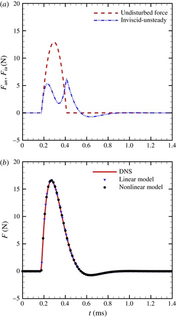
(a) Undisturbed force and inviscid-unsteady force components and (b) comparison between the current linear and nonlinear models and inviscid simulations for the axial drag force experienced by a finite-sized rigid particle due to interaction with a weak planar expansion fan.

In both cases considered, we study the flow over a finite-sized (
 $80$
mm diameter) stationary sphere. For the weak expansion case, the head of the fan first interacts with the sphere at
 $t=0.174$
ms and the tail of the expansion fan leaves the particle at time,
 $t=0.405$
ms. However, the simulation is conducted until
 $t=1.4$
ms, so that the history force (arising from the inviscid-unsteady force) is captured. As described before, since this expansion fan was generated using an initial pressure ratio of
 $1.05$
(the corresponding shock that propagates to the right has a Mach number of
 $1.01$
), the flow is nearly linear. Therefore we compare the DNS results with our linear formulation presented in (3.21). For the purposes of this study, the force predicted using (3.21) is termed the ‘linear model’. One observes from this equation that, in the inviscid limit, the only flow properties required to compute the undisturbed force are the undisturbed density and velocity averaged over the particle volume, which are shown in figure 3(a). One can observe from the figure that the gas is at a higher density before the expansion fan hits the particle and reaches a uniform state after the fan has crossed. Similarly, the axial velocity gradually rises from zero to the uniform post-shock velocity. The surface-averaged radial momentum required to calculate the inviscid-unsteady force component is presented in figure 3(b). The two force components thus computed are shown in figure 4(a), where one observes that the undisturbed force is non-zero only for the time period that the expansion fan traverses over the particle (
 $0.174\leqslant t\leqslant 0.405$
) and is non-existent at other times. The inviscid-unsteady force is comparable to the undisturbed force and more importantly exists for longer times (up to
 $t\approxeq 0.85$
) due to compressibility of the flow.
(a)
 $x$
–
 $t$
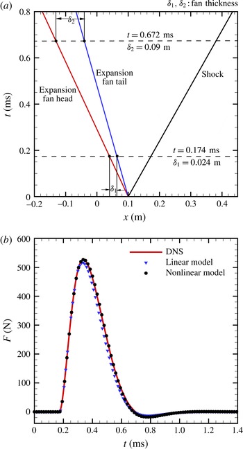
diagram for a planar shock tube with an initial pressure ratio of 2.5. The expansion fan thickness when the head of the fan first encounters the particle and when the tail of the fan leaves the particle and the corresponding times are shown. (b) Comparison between the current linear and nonlinear models and inviscid simulations for the axial drag force experienced by a finite-sized rigid particle due to interaction with a strong planar expansion fan.

The actual comparison for the weak expansion fan with the DNS results is shown in figure 4(b), where one can observe that the inviscid part of the linear model (3.21) accurately predicts the drag force for all times. Since the force formulation was derived by solving the linearized Navier–Stokes equations, the comparison is exact. Also shown in figure 4(b) is the comparison of DNS results with that of the force computed using (4.7), which will be termed the ‘nonlinear model’ in this paper. Clearly, since the flow is linear, the nonlinear terms are negligible and therefore one can compute the force either using (4.7) or (3.21), which will lead to identical results.
In the second scenario, we start with an initial pressure ratio of
 $2.5$
. In this case the thickness of the expansion fan, when it first encounters the particle at time
 $t=0.174~\text{ms}$
is 0.6 times the particle radius
 $(\unicode[STIX]{x1D6FF}_{1}=0.024~\text{m})$
, as shown in figure 5(a). Further as the tail of the expansion fan leaves the particle,
 $(t=0.672~\text{ms})$
, the fan thickness grows to 0.09 m, which is 2.25 times the particle radius. Therefore we clearly observe that the flow gradient of the ambient is of the order of the particle size. Moreover, an initial pressure ratio of
 $2.5$
leads to a shock Mach number of
 $1.215$
making the nonlinear terms in the Euler/Navier–Stokes equation significant. We first apply (3.21) (linear model) to predict the force on the particle. As can be seen from figure 5(b), the linear model does a reasonable job in capturing the force. Note that we termed (3.21) as the ‘linear model’, which is indeed true as far as the disturbance force alone is concerned. However, it must be pointed out that the undisturbed force, which involves the material derivative, in essence captures a substantial portion of the ‘nonlinear’ effect. Consequently, we achieve a reasonable comparison with the DNS data even with the linear model. Now, if the nonlinear effects are accounted for with (4.7) in the inviscid limit, we observe an excellent agreement (also shown in figure 5
b).
7 Faxén form of force for a moving particle
We will now generalize (4.7) for the case of a non-stationary particle that is undergoing arbitrary motion given by the time-dependent velocity,
 $\boldsymbol{u}_{p}(t)$
. Within the framework of the present linear analysis, we restrict the particle velocity to be only of the order of the linearized fluid velocity. In this case it is convenient to adopt the frame of reference attached to the particle. Since the frame attached to the particle is in general non-inertial, the governing linearized momentum equation written in the moving frame will involve an additional term,
 $-\unicode[STIX]{x1D70C}\,\text{d}\boldsymbol{u}_{p}/\text{d}t$
, on the right-hand side to account for the acceleration of the frame, where
 $\text{d}/\text{d}t$
is the time derivative following the particle. This additional term can be separated into that due to the undisturbed flow,
 $-\unicode[STIX]{x1D70C}_{0}\,\text{d}\boldsymbol{u}_{p}/\text{d}t$
and the contribution from the disturbed flow,
 $-\unicode[STIX]{x1D70C}_{1}\,\text{d}\boldsymbol{u}_{p}/\text{d}t$
. The former contributes to the undisturbed force which, when expressed in terms of the undisturbed ambient flow in the laboratory-attached frame, remains the same as that given in (3.3). The latter is a quadratic term (since
 $\boldsymbol{u}_{p}\approx O(\boldsymbol{u}_{1})$
) and can be ignored.
Thus, in the particle-attached frame the linearized perturbation equations (2.6) and (2.7) remain the same, except the fluid velocity is now in the moving frame of reference. Furthermore, in the solution of the scattered field, no-slip and no-penetration boundary conditions can be imposed in the particle-attached frame. Therefore, equation (4.7) applies even for a particle in arbitrary motion, except for the following reinterpretation:
 $\boldsymbol{u}^{un}$
must be replaced by
 $\boldsymbol{u}^{un}-\boldsymbol{u}_{p}$
. Making the above mentioned change the final Faxén form of the total force on a particle can be expressed as:
 $$\begin{eqnarray}\displaystyle \boldsymbol{F}^{GF}(t) & = & \displaystyle {\displaystyle \frac{4}{3}}\unicode[STIX]{x03C0}R^{3}\overline{\unicode[STIX]{x1D70C}^{un}\frac{\text{D}\boldsymbol{u}}{\text{D}t}^{un}}^{V}+6R\unicode[STIX]{x03C0}\unicode[STIX]{x1D708}\overline{\unicode[STIX]{x1D70C}^{un}(\boldsymbol{u}^{un}-\boldsymbol{u}_{p})}^{S}\unicode[STIX]{x1D6F7}(Re,M)\nonumber\\ \displaystyle & & \displaystyle +\,4\unicode[STIX]{x03C0}R^{3}\int _{\tilde{\unicode[STIX]{x1D709}}=-\infty }^{\tilde{t}}K_{iu}(\tilde{t}-\tilde{\unicode[STIX]{x1D709}};M)\left[\overline{{\displaystyle \frac{\text{D}}{\text{D}t}}}\overline{\unicode[STIX]{x1D70C}^{un}(\boldsymbol{u}_{r}^{un}-{\boldsymbol{u}_{p}}_{r})}^{S}\right]_{\tilde{t}=\tilde{\unicode[STIX]{x1D709}}}\,\text{d}\tilde{\unicode[STIX]{x1D709}}\nonumber\\ \displaystyle & & \displaystyle +\,18R^{2}\sqrt{\unicode[STIX]{x03C0}\unicode[STIX]{x1D708}}\left.\int _{\unicode[STIX]{x1D709}=-\infty }^{t}K_{vu}^{V}(t-\unicode[STIX]{x1D709};Re,M)\,{\displaystyle \frac{\text{d}}{\text{d}t}}\overline{\unicode[STIX]{x1D70C}^{un}(\boldsymbol{u}_{r}^{un}-{\boldsymbol{u}_{p}}_{r})}^{S}\right|_{t=\unicode[STIX]{x1D709}}\,\text{d}\unicode[STIX]{x1D709}\nonumber\\ \displaystyle & & \displaystyle +\,6R^{2}\sqrt{\unicode[STIX]{x03C0}\unicode[STIX]{x1D708}}\left.\int _{\unicode[STIX]{x1D709}=-\infty }^{t}K_{vu}^{S}(t-\unicode[STIX]{x1D709};Re,M)\,{\displaystyle \frac{\text{d}}{\text{d}t}}\overline{\unicode[STIX]{x1D70C}^{un}(\boldsymbol{u}^{un}-\boldsymbol{u}_{p})}^{S}\right|_{t=\unicode[STIX]{x1D709}}\,\text{d}\unicode[STIX]{x1D709}.\end{eqnarray}$$
It must be mentioned that the force expression presented above is invariant to Galilean transformation. Note that the above formulation, applicable to the force experienced by a single particle was obtained from the nonlinear version of Faxén’s force (4.7). Similar extensions to moving particles hold true for all of the force expressions mentioned in table 1. Similarly, in the low Reynolds and Mach number limit, the multiplicative correction factor,
 $\unicode[STIX]{x1D6F7}$
reduces to
 $1$
and the nonlinear forms of the kernels approach their corresponding linear limits as discussed in § 4.
Furthermore, if one were to consider a particle moving in an incompressible, homogeneous and stationary medium (
 $\unicode[STIX]{x1D70C}^{un}=\text{const.}$
,
 $\boldsymbol{u}^{un}=0$
), the above equation (7.1) reduces to:
 $$\begin{eqnarray}\displaystyle \boldsymbol{F}(t)=-6R\unicode[STIX]{x03C0}\unicode[STIX]{x1D707}\boldsymbol{u}_{p}\unicode[STIX]{x1D6F7}(Re)-{\displaystyle \frac{1}{2}}m_{f}\,{\displaystyle \frac{\text{d}\boldsymbol{u}_{p}}{\text{d}t}}-6R^{2}\sqrt{\unicode[STIX]{x03C0}\unicode[STIX]{x1D707}}\left.\int _{\unicode[STIX]{x1D709}=-\infty }^{t}K_{vu}^{S}(t-\unicode[STIX]{x1D709};Re)\,{\displaystyle \frac{\text{d}\boldsymbol{u}_{p}}{\text{d}t}}\right|_{t=\unicode[STIX]{x1D709}}\,\text{d}\unicode[STIX]{x1D709}, & & \displaystyle \nonumber\\ \displaystyle & & \displaystyle\end{eqnarray}$$
where,
 $\unicode[STIX]{x2202}/\unicode[STIX]{x2202}t$
has been reinterpreted as
 $\text{d}/\text{d}t$
. In the above,
 $Re$
and
 $M$
are now based on the relative velocity and the definitions given in (4.8) must be modified accordingly. By definition,
 $\boldsymbol{u}_{p}$
and as a result,
 $\overline{\boldsymbol{u}_{p}}^{S}$
and
 $\overline{{\boldsymbol{u}_{p}}_{r}}^{S}$
are Lagrangian quantities that are defined for the particle. As a result the total derivative of these quantities, such as
 $\overline{\text{D}}\overline{\boldsymbol{u}_{p}}^{S}/\text{D}t$
must be interpreted as
 $\text{d}\overline{\boldsymbol{u}_{p}}^{S}/\text{d}t$
.
Finally, the limitations and approximations of the above Faxén’s form of the force must be stressed. The linear version of the current Faxén’s form of the force given in (3.21) is rigorously obtained and it is exact provided all nonlinear effects are negligible (
 $Re,M\rightarrow 0$
), with no restrictions on particle size. The nonlinear generalization given above in (7.1) or in (4.7) involves important approximations, which make these nonlinear forms non-unique. For example, in the above nonlinear form, we have used the following definition:
 $\overline{\text{D}}/\text{D}t=\unicode[STIX]{x2202}/\unicode[STIX]{x2202}t+\overline{\boldsymbol{u}^{un}}^{V}\boldsymbol{\cdot }\unicode[STIX]{x1D735}$
. One could equivalently define,
 $\overline{\text{D}}/\text{D}t=\unicode[STIX]{x2202}/\unicode[STIX]{x2202}t+\overline{\boldsymbol{u}^{un}}^{S}\boldsymbol{\cdot }\unicode[STIX]{x1D735}$
. Similarly, to the linear approximation, in (3.21),
 $\unicode[STIX]{x2202}\overline{(\unicode[STIX]{x1D70C}\boldsymbol{u}_{r})}^{S}/\unicode[STIX]{x2202}t$
can be rewritten as
 $\overline{\unicode[STIX]{x2202}(\unicode[STIX]{x1D70C}\boldsymbol{u}_{r})/\unicode[STIX]{x2202}t}^{S}$
, since the surface-average and time derivative commute. Nonlinear generalization of the latter will yield
 $\overline{\text{D}(\unicode[STIX]{x1D70C}\boldsymbol{u}_{r})/\text{D}t}^{S}$
, and this form could be used in (4.7) and (7.1). Nevertheless, we applied the above modified formulations of the averaged substantial derivative to the problem of an expansion fan passing over a spherical particle considered in § 6. We observe the force computed using these different definitions to yield nearly identical results. Thus the present application is unable to pick one model form over the other. Similarly, the definition of the averaged Reynolds and Mach numbers are also subject to debate: e.g. one could define the Mach number as in (4.8) or as
 $M=\overline{|\boldsymbol{u}^{un}|/c^{un}}^{V}$
. Further investigation with other applications are needed to explore the different forms and their accuracy.
8 Conclusions
We have presented a version of Faxén’s theorem in the time domain applicable to unsteady, viscous, compressible and inhomogeneous ambient flows around a sphere. The force was initially obtained in the frequency domain by considering a plane acoustic wave (fixed wavenumber/frequency) passing over a stationary particle. The idea of density-weighted velocity was employed to compute the force using scalar and vector potentials while allowing for inhomogeneous ambient flows. The radial and tangential velocity components appearing in the force equation were expressed in terms of surface average of the undisturbed flow properties. Further, the force formulation places no restriction on the particle radius compared to the incoming acoustic wavelength. These techniques/conditions allowed us to account for any complex non-uniform ambient flow over the particle. The force was then transformed to the time domain and segregated into physically meaningful terms, namely, quasi-steady, inviscid-unsteady, viscous-unsteady and undisturbed forces. We call this force expression the ‘Faxén form of the force for spatially varying unsteady viscous compressible flows’. We also showed that the force reduces to the correct behaviour under varying limiting conditions including (i) long-time behaviour (ii) incompressible limit (iii) small particle size limit. It must be mentioned that the formulation provided as such is limited to zero Reynolds and Mach numbers but non-negligible Knudsen numbers. Nevertheless the equation of motion can be empirically extended to finite Reynolds and Mach numbers using appropriate correction factors. This results in a nonlinear Faxén’s form of the force expression. We applied this equation to model the force due to a planar expansion fan interacting with an
 $80$
mm spherical particle. We considered two cases: (i) weak expansion fan due to an initial pressure ratio of
 $1.05$
and (ii) strong expansion fan with an initial pressure ratio of
 $2.5$
. For the weak expansion fan case, our results compared very well to simulations for all times. For the second case too, the prediction was accurate if we accounted for the nonlinear terms by modifying the time derivatives following the particle to time derivatives following the fluid.
Acknowledgements
This work benefited from the US Department of Energy, National Nuclear Security Administration, Advanced Simulation and Computing Program, as a Cooperative Agreement under the Predictive Science Academic Alliance Program, under contract no. DE-NA0002378.
Appendix A. Scattering coefficients in terms of incoming flow properties
The goal here is to express the scattering coefficients,
 $S_{1}$
and
 ${S_{\unicode[STIX]{x1D708}}}_{1}$
in terms of incoming flow properties. Here we consider a plane acoustic wave to impinge on a stationary particle. Therefore, the no-slip boundary conditions dictate that:
 $$\begin{eqnarray}\displaystyle w_{1r}|_{r=R}=0,\quad w_{1\unicode[STIX]{x1D703}}|_{r=R}=0, & & \displaystyle\end{eqnarray}$$
where,
 $w_{1r}$
and
 $w_{1\unicode[STIX]{x1D703}}$
denote the radial and circumferential velocity components of the density-weighted fluid velocity, respectively. Further, since we are interested in the axial force, only the dipole/first mode (
 $n=1$
) will be considered and consequently we need to consider only the first mode of the velocity components (which are otherwise in general a summation of infinite terms). Henceforth, let us denote the flow properties corresponding to mode,
 $n=1$
, at the particle surface with superscript,
 $\widehat{\text{}}\;$
. In other words, for notational simplicity, we write for example,
 $w_{1r}|_{r=R,n=1}=\widehat{w_{1r}}$
. Based on this definition, the boundary conditions can be written as:
 $$\begin{eqnarray}\displaystyle \widehat{w_{1r}^{in}}+\widehat{w_{1r}^{sc}}=0,\quad \widehat{w_{1\unicode[STIX]{x1D703}}^{in}}+\widehat{w_{1\unicode[STIX]{x1D703}}^{sc}}=0. & & \displaystyle\end{eqnarray}$$
The expressions for velocity components in terms of velocity potentials were provided in Annamalai et al. (Reference Annamalai, Balachandar and Parmar2014) and are not repeated here for brevity. Adopting the velocity expressions we obtain from (2.16):
 $$\begin{eqnarray}\displaystyle \widehat{w_{1r}^{in}}={\displaystyle \frac{-3\text{i}C_{1}}{R}}kR{j_{1}}^{\prime }(kR)\cos \unicode[STIX]{x1D703}\text{e}^{\text{i}\unicode[STIX]{x1D714}t},\quad \widehat{w_{1\unicode[STIX]{x1D703}}^{in}}={\displaystyle \frac{3\text{i}C_{1}}{R}}j_{1}(kR)\sin \unicode[STIX]{x1D703}\text{e}^{\text{i}\unicode[STIX]{x1D714}t}. & & \displaystyle\end{eqnarray}$$
Similarly, expressions for
 $\widehat{w_{1r}^{sc}}$
and
 $\widehat{w_{1\unicode[STIX]{x1D703}}^{sc}}$
are evaluated as:
 $$\begin{eqnarray}\displaystyle \widehat{w_{1r}^{sc}}=-[f_{1}S_{1}+f_{2}{S_{\unicode[STIX]{x1D708}}}_{1}],\quad \widehat{w_{1\unicode[STIX]{x1D703}}^{sc}}=-[g_{1}S_{1}+g_{2}{S_{\unicode[STIX]{x1D708}}}_{1}], & & \displaystyle\end{eqnarray}$$
where for simplification purposes, we define the following:
 $$\begin{eqnarray}\displaystyle \left.\begin{array}{@{}c@{}}\displaystyle f_{1}={\displaystyle \frac{3\text{i}C_{1}}{R}}kR{h_{1}^{(2)}}^{\prime }(kR)\cos \unicode[STIX]{x1D703}\text{e}^{\text{i}\unicode[STIX]{x1D714}t},\quad f_{2}={\displaystyle \frac{3\text{i}C_{1}}{R}}2h_{1}^{(2)}(k_{\unicode[STIX]{x1D708}}R)\cos \unicode[STIX]{x1D703}\text{e}^{\text{i}\unicode[STIX]{x1D714}t},\\ \displaystyle g_{1}={\displaystyle \frac{-3\text{i}C_{1}}{R}}h_{1}^{(2)}(kR)\sin \unicode[STIX]{x1D703}\text{e}^{\text{i}\unicode[STIX]{x1D714}t},\quad g_{2}={\displaystyle \frac{-3\text{i}C_{1}}{R}}[2h_{1}^{(2)}(k_{\unicode[STIX]{x1D708}}R)-k_{\unicode[STIX]{x1D708}}Rh_{2}^{(2)}(k_{\unicode[STIX]{x1D708}}R)]\sin \unicode[STIX]{x1D703}\text{e}^{\text{i}\unicode[STIX]{x1D714}t}.\end{array}\right\} & & \displaystyle \nonumber\\ \displaystyle & & \displaystyle\end{eqnarray}$$
Our goal of expressing the scattering coefficients in terms of the incoming density-weighted velocity can be achieved using (A 2) and (A 4) as follows:
 $$\begin{eqnarray}\displaystyle S_{1}=A_{1}\widehat{w_{1r}^{in}}+A_{2}\widehat{w_{1\unicode[STIX]{x1D703}}^{in}},\quad {S_{\unicode[STIX]{x1D708}}}_{1}=B_{1}\widehat{w_{1r}^{in}}+B_{2}\widehat{w_{1\unicode[STIX]{x1D703}}^{in}}, & & \displaystyle\end{eqnarray}$$
where,
 $$\begin{eqnarray}\displaystyle A_{1}=\frac{g_{2}}{f_{1}g_{2}-f_{2}g_{1}},\quad A_{2}=\frac{-f_{2}}{f_{1}g_{2}-f_{2}g_{1}},\quad B_{1}=\frac{-g_{1}}{f_{1}g_{2}-f_{2}g_{1}},\quad B_{2}=\frac{f_{1}}{f_{1}g_{2}-f_{2}g_{1}}. & & \displaystyle \nonumber\\ \displaystyle & & \displaystyle\end{eqnarray}$$
Appendix B. Equivalence between the dipole component of radial velocity and surface-averaged radial velocity vector
We begin by expressing the left-hand side of (3.6) using (A 3a ) as:
 $$\begin{eqnarray}\displaystyle {\displaystyle \frac{\widehat{w_{1r}^{in}}}{\cos \unicode[STIX]{x1D703}}}\boldsymbol{e}_{z}=-3\text{i}C_{1}k{j_{1}}^{\prime }(kR)\text{e}^{\text{i}\unicode[STIX]{x1D714}t}\boldsymbol{e}_{z}. & & \displaystyle\end{eqnarray}$$
The velocity vector on the right-hand side of (3.6) can be written as:
 $$\begin{eqnarray}\displaystyle \boldsymbol{w}_{1r}^{in}=w_{1r}^{in}\boldsymbol{n}=w_{1r}^{in}\cos \unicode[STIX]{x1D703}\boldsymbol{e}_{z}. & & \displaystyle\end{eqnarray}$$
Furthermore, the radial component of the incoming velocity can be expressed using the incoming velocity potential as (Annamalai et al. Reference Annamalai, Balachandar and Parmar2014):
 $$\begin{eqnarray}\displaystyle w_{1r}^{in}=k\mathop{\sum }_{n=0}^{\infty }C_{n}(2n+1)(-\text{i})^{n}\text{j}_{n}^{\prime }(kr)P_{n}(\cos \unicode[STIX]{x1D703})\text{e}^{\text{i}\unicode[STIX]{x1D714}t}. & & \displaystyle\end{eqnarray}$$
Using the definition of surface average and substituting (B 2) and (B 3) into (3.6) (right-hand side) one obtains:
 $$\begin{eqnarray}\displaystyle {\mathcal{L}}(\overline{\boldsymbol{w}_{1r}^{in}(\boldsymbol{r},t)}^{S}) & = & \displaystyle -{\displaystyle \frac{3}{2}}\text{i}C_{1}kj_{1}^{\prime }(kR)\text{e}^{\text{i}\unicode[STIX]{x1D714}t}\boldsymbol{e}_{z}\int _{0}^{\unicode[STIX]{x03C0}}\cos ^{2}\unicode[STIX]{x1D703}\sin \unicode[STIX]{x1D703}\,\text{d}\unicode[STIX]{x1D703}\nonumber\\ \displaystyle & = & \displaystyle -\text{i}C_{1}k{j_{1}}^{\prime }(kR)\text{e}^{\text{i}\unicode[STIX]{x1D714}t}\boldsymbol{e}_{z}.\end{eqnarray}$$
In obtaining the above expression, we note that of all the terms in the summation in (B 3) only one term (
 $n=1$
) survives the integration in (B 4). In addition we have used the definition of the Legendre polynomial,
 $P_{1}(\cos \unicode[STIX]{x1D703})=\cos \unicode[STIX]{x1D703}$
. Subsequently, comparing (B 1) and (B 4), we arrive at (3.6).
Appendix C. Surface average of the radial velocity in terms of volume-averaged total velocity
In order to express the surface-averaged radial velocity in terms of the volume averages and vice versa, we start by obtaining the various terms in (3.7) and (3.15) in terms of spherical Bessel functions and Legendre polynomials. As mentioned earlier, since
 $\unicode[STIX]{x1D6EC}=-\text{i}kC_{1}$
, the equation for the incoming velocity (2.14) can be written as:
 $$\begin{eqnarray}\displaystyle \boldsymbol{w}_{1}^{in}=-\text{i}C_{1}k\exp \{-\text{i}(kz-\unicode[STIX]{x1D714}t)\}\boldsymbol{e}_{z}. & & \displaystyle\end{eqnarray}$$
Moreover, we express the exponential function in spherical coordinates as:
 $$\begin{eqnarray}\displaystyle \exp (-\text{i}kz)=\mathop{\sum }_{n=0}^{\infty }(2n+1)(-\text{i})^{n}\text{j}_{n}(kr)P_{n}(\cos \unicode[STIX]{x1D703}). & & \displaystyle\end{eqnarray}$$
Using the definition of volume average and substituting (C 2) into (C 1) we write the volume-averaged incoming velocity as:
 $$\begin{eqnarray}\displaystyle {\mathcal{L}}(\overline{\boldsymbol{w}_{1}^{in}}^{V}) & = & \displaystyle -{\displaystyle \frac{2\unicode[STIX]{x03C0}}{V^{p}}}\text{i}C_{1}k\text{e}^{\text{i}\unicode[STIX]{x1D714}t}\int _{0}^{R}r^{2}j_{0}(kr)\,\text{d}r\int _{0}^{\unicode[STIX]{x03C0}}P_{0}(\cos \unicode[STIX]{x1D703})\sin \unicode[STIX]{x1D703}\,\text{d}\unicode[STIX]{x1D703}\boldsymbol{e}_{z}\nonumber\\ \displaystyle & = & \displaystyle -{\displaystyle \frac{3\text{i}C_{1}}{R}}j_{1}(kR)\text{e}^{\text{i}\unicode[STIX]{x1D714}t}\boldsymbol{e}_{z}.\end{eqnarray}$$
It must be emphasized that in obtaining the above expression, only the
 $n=0$
term in (C 2) survives the integration in (C 3). Further, the following definitions of Bessel function and Legendre polynomials, namely:
 $$\begin{eqnarray}\displaystyle j_{0}(kr)={\displaystyle \frac{\sin (kr)}{kr}},\quad P_{0}(\cos \unicode[STIX]{x1D703})=1, & & \displaystyle\end{eqnarray}$$
were used to arrive at the above mentioned expression.
Taking the derivative of (C 1) with respect to
 $z$
and noting that,
 $\boldsymbol{r}=r\cos \unicode[STIX]{x1D703}\boldsymbol{e}_{z}$
, we have:
 $$\begin{eqnarray}\displaystyle \boldsymbol{r}\unicode[STIX]{x1D735}\boldsymbol{\cdot }\boldsymbol{w}_{1}^{in}=-k^{2}C_{1}r\cos \unicode[STIX]{x1D703}\text{e}^{-\text{i}kz}\text{e}^{\text{i}\unicode[STIX]{x1D714}t}\boldsymbol{e}_{z}, & & \displaystyle\end{eqnarray}$$
where,
 $r$
is the magnitude of
 $\boldsymbol{r}$
. Using the definition of volume average and substituting (C 2) into (C 5) we have:
 $$\begin{eqnarray}\displaystyle {\mathcal{L}}(\overline{\boldsymbol{r}\unicode[STIX]{x1D735}\boldsymbol{\cdot }\boldsymbol{w}_{1}^{in}}^{V}) & = & \displaystyle {\displaystyle \frac{6\unicode[STIX]{x03C0}}{V^{p}}}\text{i}C_{1}k^{2}\text{e}^{\text{i}\unicode[STIX]{x1D714}t}\int _{0}^{R}r^{3}j_{1}(kr)\,\text{d}r\int _{0}^{\unicode[STIX]{x03C0}}P_{1}(\cos \unicode[STIX]{x1D703})\cos \unicode[STIX]{x1D703}\sin \unicode[STIX]{x1D703}\,\text{d}\unicode[STIX]{x1D703}\boldsymbol{e}_{z}\nonumber\\ \displaystyle & = & \displaystyle 3\text{i}C_{1}kj_{2}(kR)\text{e}^{\text{i}\unicode[STIX]{x1D714}t}\boldsymbol{e}_{z}.\end{eqnarray}$$
As before, the only contribution to the integral in (C 6) is due to the
 $n=1$
term. Furthermore, the following definitions were used to arrive at the final expression:
 $$\begin{eqnarray}\displaystyle j_{1}(kr)={\displaystyle \frac{\sin (kr)}{(kr)^{2}}}-{\displaystyle \frac{\cos (kr)}{kr}},\quad j_{2}(kr)=\left(-{\displaystyle \frac{1}{kr}}+{\displaystyle \frac{3}{(kr)^{3}}}\right)\sin (kr)-{\displaystyle \frac{3}{(kr)^{2}}}\cos (kr). & & \displaystyle \nonumber\\ \displaystyle & & \displaystyle\end{eqnarray}$$
Now summing (C 3) and (C 6) we obtain:
 $$\begin{eqnarray}\displaystyle {\mathcal{L}}(\overline{\boldsymbol{w}_{1}^{in}}^{V})+{\mathcal{L}}(\overline{\boldsymbol{r}\unicode[STIX]{x1D735}\boldsymbol{\cdot }\boldsymbol{w}_{1}^{in}}^{V}) & = & \displaystyle -3\text{i}C_{1}k\left({\displaystyle \frac{j_{1}(kR)}{kR}}-j_{2}(kR)\right)\text{e}^{\text{i}\unicode[STIX]{x1D714}t}\boldsymbol{e}_{z}\nonumber\\ \displaystyle & = & \displaystyle -3\text{i}C_{1}kj_{1}^{\prime }(kR)\text{e}^{\text{i}\unicode[STIX]{x1D714}t}\boldsymbol{e}_{z},\end{eqnarray}$$
since,
 $j_{1}(kR)/kR-j_{2}(kR)=j_{1}^{\prime }(kR)$
(DLMF 2010; Olver et al.
Reference Olver, Lozier, Boisvert and Clark2010; Annamalai et al.
Reference Annamalai, Balachandar and Parmar2014). Now comparing (B 4) and (C 8) we have:
 $$\begin{eqnarray}\displaystyle {\mathcal{L}}(\overline{\boldsymbol{w}_{1r}^{in}(\boldsymbol{r},t)}^{S})={\textstyle \frac{1}{3}}{\mathcal{L}}(\overline{\boldsymbol{w}_{1}^{in}}^{V})+{\textstyle \frac{1}{3}}{\mathcal{L}}(\overline{\boldsymbol{r}\unicode[STIX]{x1D735}\boldsymbol{\cdot }\boldsymbol{w}_{1}^{in}}^{V}), & & \displaystyle\end{eqnarray}$$
which on Laplace inverse yields (3.7).
Appendix D. Volume-averaged total velocity in terms of surface-averaged velocities
Contrary to the volume-averaged incoming velocity, only the
 $n=0$
term contributes to the surface-averaged incoming velocity which may be computed as:
 $$\begin{eqnarray}\displaystyle {\mathcal{L}}(\overline{\boldsymbol{w}_{1}^{in}}^{S}) & = & \displaystyle -{\displaystyle \frac{2\unicode[STIX]{x03C0}R^{2}}{S^{p}}}\text{i}C_{1}k\text{e}^{\text{i}\unicode[STIX]{x1D714}t}j_{0}(kr)\int _{0}^{\unicode[STIX]{x03C0}}P_{0}(\cos \unicode[STIX]{x1D703})\sin \unicode[STIX]{x1D703}\,\text{d}\unicode[STIX]{x1D703}\boldsymbol{e}_{z}\nonumber\\ \displaystyle & = & \displaystyle -\text{i}C_{1}kj_{0}(kR)\text{e}^{\text{i}\unicode[STIX]{x1D714}t}\boldsymbol{e}_{z}.\end{eqnarray}$$
In order to obtain the volume average of the total incoming velocity in terms of surface-averaged quantities, we use the following recurrence relation (Annamalai et al. Reference Annamalai, Balachandar and Parmar2014):
 $$\begin{eqnarray}\displaystyle j_{1}^{\prime }(kR)=j_{0}(kR)-{\displaystyle \frac{2}{kR}}j_{1}(kR). & & \displaystyle\end{eqnarray}$$
It can be seen that (B 4), (D 1) and (C 3) are related to
 $j_{1}^{\prime }(kR)$
,
 $j_{0}(kR)$
and
 $j_{1}(kR)$
, respectively. Therefore substituting (B 4), (D 1) and (C 3) into (D 2) and simplifying we arrive at:
 $$\begin{eqnarray}\displaystyle {\mathcal{L}}(\overline{\boldsymbol{w}_{1}^{in}}^{V})={\textstyle \frac{3}{2}}{\mathcal{L}}(\overline{\boldsymbol{w}_{1}^{in}}^{S})-{\textstyle \frac{3}{2}}{\mathcal{L}}(\overline{(\boldsymbol{w}_{1}^{in}\boldsymbol{\cdot }\boldsymbol{n})\boldsymbol{n}}^{S}), & & \displaystyle\end{eqnarray}$$
which is equivalent to (3.15) on taking the Laplace inverse.
Appendix E. Limiting forms of the generalized Faxén law
In the incompressible limit (
 $c^{un}\rightarrow \infty$
,
 $\unicode[STIX]{x1D70C}^{un}=\text{const.}$
), we have
 $kR\ll 1$
. Substituting these limits into (3.9) and (3.17), and since
 $G_{qs}=9\unicode[STIX]{x1D708}/2sR^{2}$
as shown before, we obtain:
 $$\begin{eqnarray}\displaystyle G^{V}=G_{iu}={\displaystyle \frac{1}{2}};\quad G_{vu}^{S}={\displaystyle \frac{9}{2R}}\sqrt{{\displaystyle \frac{\unicode[STIX]{x1D708}}{s}}}. & & \displaystyle\end{eqnarray}$$
Substituting (E 1) into (3.20) and simplifying, (4.7) reduces to:
 $$\begin{eqnarray}\displaystyle \boldsymbol{F}^{MRG}(t) & = & \displaystyle m_{f}\overline{\frac{\text{D}\boldsymbol{u}}{\text{D}t}^{un}}^{V}+\frac{1}{2}m_{f}\overline{{\displaystyle \frac{\text{D}}{\text{D}t}}}\overline{\boldsymbol{u}^{un}}^{V}+6R\unicode[STIX]{x03C0}\unicode[STIX]{x1D707}\overline{\boldsymbol{u}^{un}}^{S}\unicode[STIX]{x1D6F7}(Re,M)\nonumber\\ \displaystyle & & \displaystyle +\,6R^{2}\sqrt{\unicode[STIX]{x03C0}\unicode[STIX]{x1D708}}\left.\int _{\unicode[STIX]{x1D709}=-\infty }^{t}K_{vu}^{S}(t-\unicode[STIX]{x1D709};Re)\,{\displaystyle \frac{\text{d}}{\text{d}t}}\overline{\boldsymbol{u}^{un}}^{S}\right|_{t=\unicode[STIX]{x1D709}}\,\text{d}\unicode[STIX]{x1D709},\end{eqnarray}$$
where
 $m_{f}=4\unicode[STIX]{x03C0}R^{3}\unicode[STIX]{x1D70C}/3$
is the mass of the displaced fluid. Note that in (E 2), (i) the undisturbed force component (3.3) in the absence of compressibility reduces to
 $m_{f}\,\text{D}\overline{\boldsymbol{u}^{un}}^{V}/\text{D}t$
, (ii) the inviscid-unsteady force in the incompressible limit, known as the added-mass force, is instantaneously experienced by the particle and does not involve a convolution integral, (iii) from (3.7), since
 $\unicode[STIX]{x1D735}\boldsymbol{\cdot }\boldsymbol{u}=0$
, the surface average of the radial velocity can be replaced by the volume average of velocity and (iv)
 $K_{vu}^{V}$
becomes identically zero in the incompressible limit. Further, it must be mentioned that this expression for force known as the MRG equation of motion, due to the disturbance flow was obtained by Maxey & Riley (Reference Maxey and Riley1983) and Gatignol (Reference Gatignol1983) in the time domain and by Mazur & Bedeaux (Reference Mazur and Bedeaux1974) in the frequency domain.
In addition, in the limit of
 $s\rightarrow 0$
, i.e. very slow ambient flow variation, only the quasi-steady force survives, leading to the nonlinear version of the classic Faxén equation of motion given by:
 $$\begin{eqnarray}\displaystyle \boldsymbol{F}^{Fax\acute{e} n}(t)=6R\unicode[STIX]{x03C0}\unicode[STIX]{x1D707}\overline{\boldsymbol{u}^{un}}^{S}\unicode[STIX]{x1D6F7}(Re,M). & & \displaystyle\end{eqnarray}$$
Further, if the ambient flow is considered to be uniform but compressible, the surface and volume averages in (E 2) can be greatly simplified and correctly reduce to the compressible BBO equation of motion, as obtained by Parmar et al. (Reference Parmar, Haselbacher and Balachandar2011). This force, denoted by
 $\boldsymbol{F}^{PHB}$
, is given by:
 $$\begin{eqnarray}\displaystyle \boldsymbol{F}^{PHB}(t) & = & \displaystyle {\displaystyle \frac{4}{3}}\unicode[STIX]{x03C0}R^{3}\unicode[STIX]{x1D70C}^{un}\frac{\text{D}\boldsymbol{u}^{un}}{\text{D}t}+6R\unicode[STIX]{x03C0}\unicode[STIX]{x1D708}(\unicode[STIX]{x1D70C}\boldsymbol{u})^{un}\unicode[STIX]{x1D6F7}(Re,M)\nonumber\\ \displaystyle & & \displaystyle +\,{\displaystyle \frac{4}{3}}\unicode[STIX]{x03C0}R^{3}\left.\int _{\tilde{\unicode[STIX]{x1D709}}=-\infty }^{\tilde{t}}K_{iu}(\tilde{t}-\tilde{\unicode[STIX]{x1D709}};M)\frac{\text{D}}{\text{D}t}(\unicode[STIX]{x1D70C}\boldsymbol{u})^{un}\right|_{\tilde{t}=\tilde{\unicode[STIX]{x1D709}}}\,\text{d}\tilde{\unicode[STIX]{x1D709}}\nonumber\\ \displaystyle & & \displaystyle +\,6R^{2}\sqrt{\unicode[STIX]{x03C0}\unicode[STIX]{x1D708}}\left.\int _{\unicode[STIX]{x1D709}=-\infty }^{t}K_{vu}^{S}(t-\unicode[STIX]{x1D709};Re,M)\,{\displaystyle \frac{\text{d}}{\text{d}t}}(\unicode[STIX]{x1D70C}\boldsymbol{u})^{un}\right|_{t=\unicode[STIX]{x1D709}}\,\text{d}\unicode[STIX]{x1D709}.\end{eqnarray}$$
Note that in (E 4), the spatial averages are not necessary since the spherical particle is taken to be much smaller than the scale of the ambient flow variation. In other words on the scale of the particle, the ambient flow can be taken to be uniform. In (E 4) the incoming flow quantities
 $(\unicode[STIX]{x1D70C}\boldsymbol{u})^{un}$
and
 $\text{D}(\unicode[STIX]{x1D70C}\boldsymbol{u})^{un}/\text{D}t$
are to be interpreted as those evaluated at the particle centre. The inviscid-unsteady force continues to remain as a history force due to the effect of compressibility. This force expression was presented in the frequency domain by Zwanzig & Bixon (Reference Zwanzig and Bixon1970). In addition, if one assumes the flow to be incompressible in addition to being uniform, (E 4) reduces to the standard BBO equation given by:
 $$\begin{eqnarray}\displaystyle \boldsymbol{F}^{BBO}(t) & = & \displaystyle m_{f}\frac{\text{D}\boldsymbol{u}^{un}}{\text{D}t}+{\displaystyle \frac{1}{2}}m_{f}\frac{\text{D}\boldsymbol{u}^{un}}{\text{D}t}+6R\unicode[STIX]{x03C0}\unicode[STIX]{x1D707}\boldsymbol{u}^{un}\unicode[STIX]{x1D6F7}(Re,M)\nonumber\\ \displaystyle & & \displaystyle +\,6R^{2}\sqrt{\unicode[STIX]{x03C0}\unicode[STIX]{x1D707}}\left.\int _{\unicode[STIX]{x1D709}=-\infty }^{t}K_{vu}^{S}(t-\unicode[STIX]{x1D709};Re,M)\,\frac{\text{d}\boldsymbol{u}^{un}}{\text{d}t}\right|_{t=\unicode[STIX]{x1D709}}\,\text{d}\unicode[STIX]{x1D709}.\end{eqnarray}$$