

Introduction
Life tables (e.g. Morris, Reference Morris1959; Varley & Gradwell, Reference Varley and Gradwell1970; Southwood & Henderson, Reference Southwood and Henderson2000), demography (Carey, Reference Carey1993, Reference Carey2001) and phenology (e.g. Logan, Reference Logan1988; Regniere, Reference Regniere1984; Wagner et al., Reference Wagner, Wu, Sharpe and Coulson1984) are among the most important research fields in insect population ecology and pest management. Life tables are particularly important because they are both an experiment scheme (design) to collect comprehensive population demographic data as well as a set of mathematical approaches to analyze the collected data. The life table originated in the study of human demography and life insurance, and its history can be traced back to the seventeenth century (1660s) when the probability theory was still in its early development (see ‘Chapter 8: The Probabilistic Interpretation of Graunt's Life Table’ by Hald, Reference Hald2003). Since its introduction into insect population studies during the early 1960s, the life table has become a popular technique in entomological research (Morris, Reference Morris1959; Varley & Gradwell, Reference Varley and Gradwell1970; Southwood & Henderson, Reference Southwood and Henderson2000; Carey, Reference Carey1993, Reference Carey2001). However, the closely associated survival analysis, which revolutionized the rigorous analysis of life tables in actuarial science, human demography, biomedicine and public health beginning in the 1960s, has hardly been applied to life table analysis for insect populations. Much of the life table analysis in entomological research is limited to simple percentage rates, such as mortality or fraction of time survived. This kind of simple analysis usually does not consider underlying probability distributions of parameters or samples and may lack a sound statistical basis. As pointed out by Cox & Oakes (Reference Cox and Oakes1984), the calculation of survival rates (such as in traditional life table analysis) as simple survival proportions is possible only if no individual is censored, and violation of this restriction can lead to some absurdities.
In approximately the same period when the life table was introduced into entomology, survival analysis began to develop. This development happened to be strongly related to life table technique initially, and one may even say that survival analysis was initially developed to solve the problems in life table analysis. This connection between survival analysis and life table is clearly demonstrated by a few classic papers in survival analysis, notably Kaplan & Meier (Reference Kaplan and Meier1958) and Chiang (Reference Chiang1960). After more than four decades' development, survival analysis has not only established itself as one of the most active research fields in mathematical statistics, but also become a de facto standard in biomedical research, such as clinical data analysis and public health research (Hougaard, Reference Hougaard2000; Kalbfleisch & Prentice, Reference Kalbfleisch and Prentice2002; Lawless, Reference Lawless2003; Ibrahim et al., Reference Ibrahim, Chen and Sinha2005).
Starting in the late 1980s and early 1990s, entomologists began to discuss the problems associated with traditional hypothesis testing, such as ANOVA (ANalysis Of VAriance) and significant testing (e.g. Young & Young, Reference Young and Young1991); some entomological studies indeed explored a few ad hoc studies on the application of survival analysis (Braner & Hairston, Reference Braner, Hairston, McDonald, Manly, Lockwood and Logan1989; Curry & Feldman, Reference Curry and Feldman1987; Schaalje & van der Vaart, 1989; Schaalje et al., Reference Schaalje, Johnson and van der Varrt1992). However, the first comprehensive application of survival analysis to entomology seemed to occur in the late 1990s (Ma, Reference Ma1997). Ma's (Reference Ma1997) dissertation started with a carefully designed insect demography experiment (in total, 1800 RWA reared under 25 different treatments in laboratory) and introduced survival analysis to the study of the three aforementioned fields in insect population ecology, i.e. life tables, demography and phenology. Furthermore, a survival-analysis-based simulation model for RWA population dynamics was built from the same research. In this paper, the life table analysis and part of the demographic study with survival analysis approach, originally conducted by Ma (Reference Ma1997), are reported. As a side note, the results on the other topics (survival, development, simulation model) are reported in Ma & Bechinski (Reference Ma and Bechinski2008a,Reference Ma and Bechinskib, Reference Ma and Bechinski2009). In the last decade, more applications of survival analysis in entomology appeared in literature (e.g. Ma, Reference Ma1997; He & Alfaro, Reference He and Alfaro2000; Tanhuanpa & Ruohhoma, Reference Tanhuanpa and Ruohhoma2001; Velema et al., Reference Velema, Hemerik, Hoddle and Luck2005; Fox & Kendall, Reference Fox and Kendall2006; Ma & Bechinski, Reference Ma and Bechinski2008b, Reference Ma and Bechinski2009), including an excellent survey on survival analysis in ecological research (also with some tutorial materials) by Zens & Peart (Reference Zens and Peart2003). Overall, my opinion is that survival analysis should become a widely applied standard statistical tool-box for much of the entomological research. It should be noted that survival analysis is beyond a single or single group of statistical tool(s); instead, it has developed all major counterpart branches of modern statistics, from Bayesian survival analysis (Ibrahim et al., Reference Ibrahim, Chen and Sinha2005) to multivariate survival analysis (Hougaard, Reference Hougaard2000; Ma & Krings, Reference Ma and Krings2008a,b).
I attempt to achieve three objectives as stated in the abstract, i.e.: (i) addressing a fundamental issue in many entomological studies – censoring or incomplete observations; (ii) demonstrating the application of survival analysis to analyze insect life tables; and (iii) applying survival analysis for hypothesis testing. Since, to the best of my knowledge, this study seems still the first application of survival analysis to the study of insect life tables, an extremely brief introduction on the fundamental concepts of survival analysis, as well as its primary advantages when applied to entomology, are presented in the next section.
Experiment data and statistical methods
Laboratory experiments
RWA development and survival data were obtained from laboratory experiments described in detail in Ma (Reference Ma1997) and Ma & Bechinski (Reference Ma and Bechinski2008a,Reference Ma and Bechinskib). This is a typical insect demography study under laboratory conditions. The experiments investigated the influence of a factorial arrangement of five temperature and five barley plant-growth stage regimes on RWA development and survival in laboratory growth chambers. For each of the 25 treatments, the developmental timing, lifespan and daily nymphal production of 72 RWA individuals (total 25×72=1800 RWA) were observed. The five temperature regimes were 1–8°C, 10–17°C, 16–23°C, 21–28°C and 26–33°C, fluctuating on a 14:10 h rectangular-wave cycle. Photoperiod was 14:10 (light:dark) for all treatments, with the higher constant temperature occurring during the light phase and the lower temperature during the dark phase. Mean temperatures weighted by photoperiod were 5.1, 14.1, 20.1, 25.1 and 30.1°C, respectively. Barley plant stages were two-leaf, tillering, flag leaf, inflorescence and soft dough, corresponding to the scale of Zadoks et al. (Reference Zadoks, Chang and Konzak1974) as stages 12, 23, 39, 59 and 85.
Survival analysis – study of time-to-event random variables with censoring
Censoring and problem description
More than a dozen monographs on survival analysis have been published (e.g. Cox & Oakes, Reference Cox and Oakes1984; Hougaard, Reference Hougaard2000; Kalbfleisch & Prentice, Reference Kalbfleisch and Prentice2002; Lawless, Reference Lawless2003; Ibrahim et al., Reference Ibrahim, Chen and Sinha2005). In survival analysis, counterparts exist for many of the procedures and methods in traditional statistics, including Bayes survival analysis (Ibrahim et al., Reference Ibrahim, Chen and Sinha2005) and multivariate survival analysis (e.g. Hougaard, Reference Hougaard2000; Ma & Krings, Reference Ma and Krings2008a,Reference Ma and Kringsb). Here, we can only briefly introduce what is needed for the objectives of this article. In survival analysis, one is interested in a group or groups of individuals characterized by a defined point-event, often called a failure, which occurs after a length of time called the failure time (or survival time). The failure or survival time can be described with a positive random variable, also known as time-to-event random variable. An individual can only fail once; for example, a RWA can die only once. (However, this is only true in univariate survival analysis, which we are limited to in this paper). Entomological examples of failure times include the emergence of an insect from a stage or the death of an insect. To determine failure times, there are three requirements: a time origin must be defined unambiguously; a scale for measuring the failure time must be identified; and the meaning of failure must be clear (Cox & Oakes, Reference Cox and Oakes1984). A special challenge in analyzing time-to-event (i.e. survival or failure time) data is the observation censoring, or the incomplete observation of survival times. An individual insect in an experiment may be lost after a period of observation due to unexpected reasons, such as escape or accidental death. In other situations, the censoring may simply be due to the reality that observing all individuals for the full course to failure is too costly, time-consuming or unacceptable. Still, in other cases, the process may have been going on but unobserved or unperceived prior to the study, for example, the arrival of a new natural enemy, or the spread of an epidemic disease. In the latter cases, an artificial start date (e.g. the discovery time) has to be specified. The three scenarios above may serve as typical examples for the three standard types of censoring in survival analysis: random censoring, right censoring (truncate) and left censoring (truncate), respectively. There is another subtle but hardly avoidable censoring mechanism in many biological studies, that is, the censoring due to the continuous nature of a time process and the discrete nature of limited sampling intervals, which makes the precise recording of the survival times for all individuals in an experiment impossible. This kind of censoring is called interval censoring in survival analysis. With interval censored data, each event time is then only known to lie in some interval, and the precise time to an event is often not known due to the limited sampling points.
The above-described censoring mechanisms are relatively easy to identify. It seems to us that the following scenario in the study of insect development is more elusive. Let us assume there are two cohorts of RWA individuals reared under different temperatures and their developmental durations for each stage are observed. Each individual should experience one of two events: either development from one stage to the next or death before completing development within a particular stage. Suppose we are to compare development durations between those two cohorts. One immediate question is how to deal with those individuals that died prematurely before completing the development. Should they be counted in the samples for statistical testing with ANOVA? Obviously, those individuals that died can contribute partial information about the developmental rate because they survived for a period of time. But on the other hand, it is not possible to know how long they would have lived in the stage. If they are excluded from the analysis, which is usually the case, their partial information is lost. Common statistical tests, such as ANOVA, cannot handle the partial information if they are included in the samples. Therefore, whether to include individuals that died before completing a stage in a study of insect development is a dilemma for traditional statistics.
The decision to include or exclude those prematurely dead individuals is not trivial because the survival patterns of two cohorts under different temperatures may be different, which implies that simple exclusion from both samples may not treat the two different samples fairly. There are two additional problems that further complicate the situation: individual variation in development rate and survival capability (or their adaptability to environment), and possible non-independence between the events of development (molting or emergence) and death. From this discussion, it is clear that the partial information should not be excluded from statistical analysis, and the only problem is how to process it if not excluded. The above dilemma disappears when we apply survival analysis because survival analysis has been developed to study a special type of random variables (named survival time, lifetime, failure time, or time-to-event random variable, and used interchangeably in literature) with censoring. Besides, survival analysis tests the difference between two samples by assessing the survivor functions, which can effectively consider the individual variability and the whole survival process.
It is fully justified to treat dead individuals as censored to study development because it allows partial development information (from those that died before completing the development of the stage under investigation) to be utilized. Of course, when the objective changes to the study of survival from development, treating prematurely dead individuals as censored loses its justification. Therefore, there is no need to treat the concept of censoring literally. The bottom line is that by treating dead individuals as censored in the study of development, we find a solution for the dilemma previously rarely recognized. Certainly, other kinds of censoring caused by events, such as escape and accidental killing (random censoring), discontinuation of observation (right censoring), or the outbreak of an epidemic with unknown occurrence date (left censoring), may still happen in insect population studies. Our opinion is that, for the unique capability to handle the censoring issue alone, survival analysis should possess very promising potentials in entomological research because we are not aware any other known method that may solve the dilemma identified previously.
Basic definitions in survival analysis
Suppose that the ith individual in a sample of n individuals has a failure time of T i; in the absence of censoring, T i is a positive random variable. Also, assume there is a period of observation C i such that observation on the ith individual ends at C i if failure has not yet taken place. The observation will consists of X i=min (T i, C i), together with the indicator variable V i=1 if T i=C i (uncensored) or V i=0 if T i>C i (censored). In some applications, all the C i will be known, such as when the cause of censoring is the planned ending of observation at a predetermined time. This type I censoring (or time censoring) occurs only when failure has not happened before terminating the study. In type II censoring (also called order statistic censoring), observation ceases after a predetermined number of individuals fail so that C becomes a random variable (Cox & Oakes, Reference Cox and Oakes1984; Kalbfleisch & Prentice, Reference Kalbfleisch and Prentice2002; Lawless, Reference Lawless2003). One of the most important advantages of survival analysis over other statistical methods is the ability to process censored information.
Let T (or T i) be a non-negative random variable representing the failure (survival) time of an individual from a homogeneous population. The probability distribution of T can be specified in several ways, three of which are particularly useful in the context of survival analysis: the survivor function, the probability density function and the hazard function. Each function is convertible into the others. The survivor function is the probability that a subject survives to at least a specified time or longer, without a failure. The hazard function is the instantaneous rate of failure at a specified time, given that the subject will survive at least that specified time point without a failure response. In the case of RWA development, the survivor function is the probability an individual has not yet developed to the next stage until some specified time point, and the hazard function is the instantaneous rate of development at a specified point. Similarly, in the context of RWA survival, the survivor function is the probability that the individual will not die before time t; the hazard function is the instantaneous rate of death given that the individual will survive at least to time t. The probability density function has the same meaning as that in traditional statistics.
The survivor function S(t) is formally defined as the probability that failure time T is at least as great as some value t; that is,

Note the similarity between the survivor function and the following distribution function of random variable T:


The remaining two ways of specifying the probability distribution of survival time, the probability density functions and hazard functions, are most readily described separately for discrete and continuous T. For continuous (absolute) survivor time T⩾0, the probability density function (p.d.f) of T is

The hazard function specifies the instantaneous rate of failure at T=t conditional upon survival to time t and is defined as:

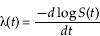
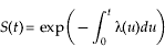
The relationships among S(t), f(t), and λ(t) are expressed as
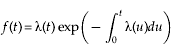
If T instead is a discrete random variable taking values x1<x2<… with associated probability function

then the survivor function is:
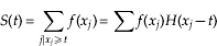
where H(x)=0 if x<0 and H(x)=1 if x⩾0.
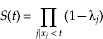
The hazard at x j is defined as the conditional probability of failure at x j,

The survivor function is:
The pth quantile of the distribution of T is the smallest t p such that,

If T is a continuous random variable, then the pth quantile can be found by solving S(t p)=1−p.
The median lifetime (mlt) is the 50th percentile t 0.5 of the distribution of T and is obtained by solving the following equation:

Data analysis
For analysis, we divided the life cycle of RWA into the following six stages: first instar (1st), second instar (2nd), third instar (3rd), fourth instar (4th), fifth instar (5th), and lifespan from birth to death (lifespan). For each stage except lifespan, there are two random variables, T e and T d, where T e is development time from the beginning of the stage until the individual exited the stage alive and where T d is the time from the beginning of the stage until the individual died within the stage. When comparing development times (T e) across treatment, T d values can be treated as censored data. Survival analysis excels other statistical methods in processing the partial information about RWA development embedded in T d.
Treatment effects on RWA development time and survival were analyzed by using the life tables and survivor functions procedures of BMDP 1L program for survival analysis (BMDP, 1993). The data format required by BMDP 1L program is as follows: serial no. (for each RWA individual), temperature, plant-stage, RWA-stage (1st–5th instars, lifespan), T (observation time), state (1 for responded, 0 for censored). These are the fields of a full data record. The first four fields are self-explaining. The last filed, State, which takes a value of either 1 or 0, with 1 representing individuals that completed development and 0 representing individuals that died within the stage. The filed T is generally called response time; its exact meaning depends on the state value. For RWA nymphs, if state is 1, then response time records developmental time in days; if state is 0, then response time records exit time due to death or other censoring reasons. For the lifespan, the state variable of 1 implies the normal death of the individual, and the state variable of 0 implies censored or exited the observation abnormally, e.g. due to an accident caused by the observer.
With this data format, the analysis conducted by BMDP 1L program proceeds as follows. First, the life table for the response time (failure time) is constructed for each data set, and the values of survivor function and hazard function (formulae (1) (5) (10) (11)) are calculated. The BMDP 1L program calculates other useful statistics, such as estimates of 75th, 50th (median response time), and 25th quantile of failure times and their standard errors. Finally, the most important part of BMDP 1L procedure: survivor functions across samples are compared by using the following four statistics: (i) Mantel-Cox statistic (Mantel, Reference Mantel1966), also known as the log-rank test, which gives equal weights to all observations; (ii) Breslow statistic (Breslow, Reference Breslow1974), which gives greatest weights to early observations and is less sensitive than the Mantel-Cox statistic to late-occurring events when few individuals remain; (iii) Tarone & Ware (Reference Tarone and Ware1977) statistic, which provides a compromise between the Mantel-Cox and Breslow statistics by using an intermediate weighting scheme; Tarone & Ware (Reference Tarone and Ware1977) suggested that their test maintains greater statistical power across a wider range of alternatives than do the other two tests; (iv) Peto-Prentice statistic (Prentice & Marek, Reference Prentice and Marek1979), which weights the difference between observed and expected responses at a particular time point by using an estimate of the survivor function. In contrast, the Breslow and Tarone-Ware statistics weights differences by using functions of the size set at that particular time point.
We use the above four statistics to test whether or not temperatures or plant-growth stages influence the development and survival of RWA. We used the so-called stratified testing, which is similar to the grouping in conventional statistics such as ANOVA. The advantages of stratifications are explained in the result section.
Results
Survival analysis approach to life table analysis
The response time T, which equals either T e (if the individual emerged or molted) or T d (if the individual died within the stage), will be described by survivor or hazard function. This unified designation of the events of emergence (development) and death (survival) with response variable (which is often interchangeably used with failure time, survival time, lifetime or, simply, time-to-event random variable) is crucial for our adoption of survival analysis. It has two immediate advantages. The first advantage is that it allows the modeling of both development and death with a single unified model structure. In other words, the same survivor function (or hazard function, which can convert from each other) can be used to model either development or survival (Ma & Bechinski, Reference Ma and Bechinski2008b, Reference Ma and Bechinski2009). When using the standard software package, such as BMDP, this can be accomplished with a simple switch of the status (state) variable that specifies which of the events (emergence or death) is the response variable. The second advantage is that it resolves the previously discussed dilemma; by treating T d as censored variable and T e as response variable, those RWA nymphs that prematurely died before the next molting contribute partial information to the analysis.
We use the combined datasets of all 25 treatments to conduct life table analysis. The BMDP 1L program was used to perform the analysis and the results are summarized in tables 1–3 and figs 1 and 2 to illustrate the approach.
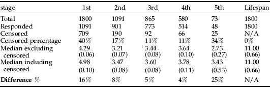
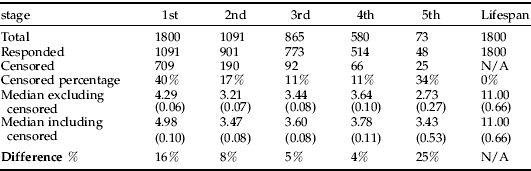
Censorings of 1800 RWA for each instar.
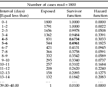
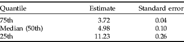
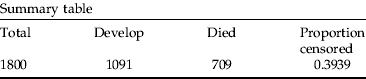
Life table with survival analysis for development of 1800 1st instar RWA.

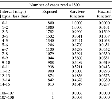
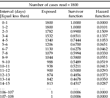
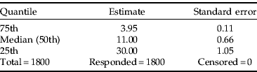
Life table with survival analysis for the lifespan survival (mortality) of 1800 RWA.
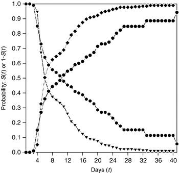
Survivor functions for the development and survival of 1800 RWA first instar nymphs (– -▾– -, S(t) for development; ····✦····, [1−S(t)] for development;  , S(t) for survival; –•–, [1−S(t) for survival]).

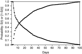
Survivor function for the lifespan survival (mortality) of 1800 RWA (––•––, survivor function S(t); ––▪––, 1−S(t)=Mortality).

This section is divided into three subsections: censoring issue, survival analysis and life table approach to RWA development, and survival analysis and life table approach to RWA survival.
Censoring issue
While the censoring events, such as the stop of observations or human errors, are certainly possible in entomological study, they did not occur in our experiments. The results in table 1 reflect two censoring events. The first one is introduced to deal with the dilemma whether to include those that prematurely died before the next emergence from the stage under investigation, as explained previously. Essentially, we take advantage of the capability of survival analysis in processing the partial information to resolve the premature death issue in analyzing insect development. This type of censoring is reflected in the first three rows in table 1. For example, we started with 1800 newly born RWA nymphs, 1091 of which successfully molted and survived (developed) to the 2nd instar, but 708 individuals died before ever reaching the 2nd instar. Nobody can ever know how long it would take for them to advance to the next stage had they not died. However, if they ever had the opportunity to advance, they would need at least T d days, that is, the response variable T>T d. This can be considered as right censoring. With the traditional approach to studying insect development, it is a dilemma whether to include these censored individuals. Obviously, either inclusion or exclusion will introduce bias to the estimation of development parameters, such as median development duration. Survival analysis is developed with the built-in inference mechanisms to ‘extract’ the partial information from the censored observations based on the asymptotic likelihood theory or, more recently, on the counting stochastic process.
We now try to explain the second censoring mechanism hidden in insect development study data. Notice that in table 1, one may expect that the total number of the 3rd instar should equal the ‘responded’ (developed or emerged) in the 2nd instar, just like in the transition from the 1st instar to the 2nd instar. That is, 1091 for the total of the 2nd instar and 910 for the 3rd instar. However, the total (or starting number) of the 3rd instar is 865 rather than 901 as one might expect. Then where were the 36 (901–865) RWA nymphs? Similarly, there were 193 (773–580), 441 (514–73) missing in the transitions from the 3rd to 4th and 4th to 5th, respectively. These individuals did not die during the corresponding periods, since the dead nymphs are already accounted for in the ‘censored’ row, for example, 709, 190, 92, 66, 25 died during the 1st, 2nd, …, 5th instar, respectively. This discrepancy is due to the biological phenomena that insect nymphs (larvae) may have different number of instarships. In the case of RWA, most nymphs have 4 instars, but 2, 3 and 5 are also possible. In other words, some RWA may enter into the reproductive stage after 1, 2, 3 or 4 molts, with most beginning to reproduce after 3 molts. The problem is that we usually do not know how many instars a RWA nymph will have until we observe the individual RWA reaching adulthood and beginning to produce progenies. What is even more elusive is that, if a RWA died prematurely before reaching the adult stage, we may never know how many instars it may have had if it was given the chance to live the full course to adulthood. Obviously, this censoring, just like the first type of censoring due to premature death, is unavoidable even with perfect experiment design and perfect execution of the design.
It is important to distinguish the two types of censoring mechanisms we identified here. The commonality is that both are often beyond our control since both of which are determined by the natural processes in insect life cycles. However, the first type of censoring can be and should be processed with survival analysis effectively, because survival analysis can ‘extract’ the partial information from those prematurely dead individuals. However, survival analysis cannot help with the second type of censoring. Actually, those individuals which skipped the current instar and directly advanced to the adult stage should be excluded from data analysis because, once the experiments are finished, it is known how many instars they should have and they do not carry partial information.
The next question is how significant the difference could be by excluding the censored observation vs. utilizing survival analysis so that the partial development information is harnessed. The rows ‘Median excluding censored’ and ‘Median including censored’ in table 1 are from the BMDP 1L package analysis. The former is computed by excluding the censored RWA individuals in the life table analysis (this is essentially the same as the traditional treatment in life tables in entomology), and the latter from the normal survival analysis (that is, the censored records are incorporated in survival analysis). The median refers to the time when survivor function S(t)=0.5 (equation 13) and will be explained further in the next section. Table 1 exhibited that the differences between the two approaches range from 4–25%. It is expected by the theory of survival analysis, and intuitively obvious, that the severer the censoring, the more significant the difference in results. It also makes intuitive sense that the procedure excluding censored individuals should result in smaller median estimates than that including censored individuals, because it is expected that those that died prematurely must be less healthy and less vigorous and, therefore, develop slower than those that survived and developed to the next stage. Therefore, incorporating the censored individuals should prolong the development of a population and results in a large value of the median development. This is the case in table 1. The next section will also show how the medians are computed.
It should be pointed out that the last column (death or lifespan) does not have censoring (although it is still possible due to reasons such as accidental death caused by human errors or escapes). However, the dilemma exhibited in the development study does not exist because every RWA dies ultimately and only dies once. The analysis of death or lifespan is essentially the same as the ‘survival’ or ‘mortality’ analysis in traditional entomological life table analysis.
Survival analysis and life table approach to RWA development
Survival analysis can be applied to analyzing life tables. Unlike in traditional life table analysis in entomology where life table analysis is used for analyzing mortality or survival only, we also apply the life table analysis for studying insect development with survival analysis. Both the emergence (marked by molting) and death are time-to-event random variables and they are mathematically equivalent. Therefore, mathematically, the life table and associated survival analysis procedures can be used to analyze both insect development and survival (mortality). Indeed, the new approach to development with survival analysis possesses a unique advantage, which we have discussed previously, dealing with the almost unavoidable censoring due to the premature death.
When utilizing standard survival analysis package such as BMDP 1L, the only difference in analyzing development and survival (death) lies in the designation of the response variable and corresponding status (state) variable (BMDP, 1993; Ma, Reference Ma1997). We performed such analyses for RWA and listed the results for the 1st instar development as an example in table 2, and we omit the results for other stages to save page space. The first two columns of table 2 specify the time interval in days. The column EXPOSED gives the equivalent number of RWA individuals alive at the beginning of the interval. In the context of survival analysis, these individuals were ‘exposed’ to the ‘risk’ of completing development; it is the number of RWA that had a chance to complete development. The column SURVIVOR Function (defined by equation 1 or 10) is the cumulative proportion of individuals yet to develop into the next instar (stage) at the beginning of the ith interval. For the analysis of survival or mortality, the survivor function is the same as in the traditional life table; it is the cumulative of individuals that are alive at the beginning of the interval. The HAZARD column is the estimated hazard function (equation 5 and 11) values in each time interval. The other columns are self-explained. The estimates of 75th, 50th (median development) and 25th percentiles of the survivor function are listed below the life table. Note that the 50th percentile of the survival function (or the median of the survivor function) is not the time to which 50% of the individuals wait to emerge. This would only be true when no individuals died (censored) before that time; similar interpretations hold for the other two quantiles. At the end of table 2 is listed the total number of RWA individuals used in the analysis, the numbers that completed development (emerged) and that died (censored), and the proportion of observations censored due to death.
We omitted the life table for the survival of the 1st instar RWA, but included its survivor functions curves for both development and survival in fig. 1. Figure 1 illustrates the survival functions for both development and survival (mortality) of RWA 1st instar. We also graphed the 1–S(t) for both survivor functions, which might be more intuitive for measuring insect development. For example, it is the (cumulative) probability that an individual has finished development of the stage at time (t) or the cumulative percentage of individuals in a population that have finished the development.
Survival analysis and life table approach to RWA survival
Table 3 is a life table we constructed for 1800 RWA lifespan (lifetime) survival with BMDP 1L program. The table headers and formats are the same as explained in the previous section, except that the response variable is death, rather than development. The only difference is that no censoring is involved. Figure 2 is the graph for survivor function S(t) and 1–S(t).
Survival analysis, when applied to mortality (survival) analysis with the life table, has three significant differences from traditional approaches in life table analysis in entomology, although the results look very similar in presentation. The first is the processing of censored observation. The second difference is that survival analysis utilizes standard survivor function and hazard function defined in equations 1–12 rather than simple proportion or rates. As pointed out by Cox & Oakes (Reference Cox and Oakes1984), the calculation of survival rates (such as in traditional life table analysis) as simple survival proportions is possible only if no individuals are censored, and violation of this restriction can lead to some absurdities. We believe Cox & Oakes' (Reference Cox and Oakes1984) warning, although it was made in the context of biomedicine more than two decades ago, is still of relevance for the life table analysis in entomology.
In laboratory experiments such as the RWA experiments reported here, avoiding censoring in the context of mortality analysis is possible (it is not avoidable for development study as we demonstrated in the previous section), censoring is hardly avoidable for field studies even in mortality analysis. The third difference, which is beyond the scope of this article, is that survival analysis offers rich modeling approaches, including both parametric, such as Weibull distribution, and semi-parametric models, such as Cox's proportional hazard model. These models can be utilized to build survival function models with time-dependent covariates (environmental factors); they can be directly incorporated into a simulation model for insect population dynamics (Ma & Bechinski, Reference Ma and Bechinski2008b). When applied to building a complex simulation model, the advantage of utilizing a unified survival analysis model to describe both development and survival is profound.
Hypothesis testing
Since four statistics reached the consistent results, we only listed the statistics for the Mantel-Cox Statistic Peto-Prentice Statistic in the following to save space, but full results were documented in Ma (Reference Ma1997). When multiple factors are involved, such as temperature and host plant-growth stage, the stratified analysis that classifies data into strata according to values of the covariate (i.e. temperature strata when testing for plant-growth stage effect or plant-growth stage strata when testing for temperature effects) has several advantages and is the best option. This is similar to the grouping in ANOVA. The data in each stratum can be summarized as survivor and hazard functions, but the tests combine the effects from each stratum and produce one overall test statistic for comparing survivor functions across treatment groups. Hence, the full data set can be used to compute the test statistics, and possible effects due to covariates other than the treatment are controlled by stratification. In our study, the data set consisting of all 1800 RWA individuals can be used in the stratification approach.
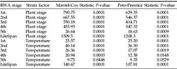
To test the effects of temperature on the development and survival of RWA, the whole data set of 1800 individuals under 25 different temperature and plant-growth stage combinations (treatments) were stratified with plant-growth stage. Similarly, to test equality of survivor functions across plant stages, we used temperature to stratify the data set. Both set of test results are summarized in table 4 but can be distinguished from each other by the strata factor column.
Statistical tests for the equality of RWA survivor functions with stratifications.

The resulting statistics and P-values listed in table 4 show that both temperature and plant-growth stages strongly influences the development and/or survival of RWA and that the p-values reject the hypothesis of equal survivor functions in all cases. Note that values of statistics from tests for temperature effects are much larger than those for plant stages effects and the p-values (risk levels) are generally lower for temperature effects testing than for plant stage. This implies that temperature effects are more significant than the effects of plant-growth stage on RWA development and survival.
In general, the stratification improves the sensitivity of the hypotheses tests; it allows the direct use of a larger data set while controlling effects of other covariates and producing one single comprehensive statistic for each covariate tested.
We advocate using survival analysis as an alternative to the conventional techniques such as ANOVA. We particularly wish to emphasize two advantages of survival analysis: censoring handling as well as the dynamic nature of the testing statistics. The latter means that the statistics in survival analysis reject or accept a hypothesis by testing the equality (or inequality) of survivor functions, which are time-dependent and are much more comprehensive than statistics such as F-values or t-values in ANOVA or significance tests.
Discussion
The methods demonstrated in this paper, such as survival analysis approach to life table analysis as well as hypothesis testing, are of general applicability to insect population data that involves any time-to-event random variables. Generally, there are two major categories of data from observing and recording a time-dependent process: one is the time-series data and the other is the time-to-event data. In entomological studies, field population dynamics data are often collected in time series; but, in laboratory demography, life tables, bioassay and many other studies, the dominant variables are often time-to-event observations such as molting, emergence, longevity, death time after chemical treatment, the occurrence times of behavior or physiological events, etc. An equally ubiquitous phenomenon associated with time-to-event random variables is the censoring or incomplete observations. From these two ‘trademarks’ of survival analysis, it is obvious that survival analysis should become a major statistical tool for entomological research, just like in other fields, such as biomedicine, where survival analysis has become a de facto standard.
Often, when a new statistical method is introduced to a field, it should be compared with the existing methods. Although we dedicate much of the first part in the ‘Results’ section to compare survival analysis with the existing life tables in entomology, we found that the comparison is somewhat difficult for the following reason: the traditional statistics is not able to handle censoring. It might be that, unless the true values of biological parameters are available, the comparison is similar to comparing apples with oranges, although both have the common nutrition value of fruits. Given the limitation of direct comparison, in this article we tried to first examine the mathematical problems abstracted from the issues which survival analysis addresses in biomedicine and public health research, such as censoring, life tables, the nature of time-to-event random variables, covariates, survivor function, hazard function, quantile and median. We argue that these concepts, mechanisms and problems exist in entomological research with the same or very similar biological meanings; further, they are essentially the same in both domains, when abstracted into mathematical formulations. For example, the survival of patients vs. the survival of insects, effects of drugs vs. effects of pesticides, life tables of human population vs. life tables of insects are essentially the same mathematically. Based on this observation, we suggest that the comparative study of survival analysis with the existing statistical approaches should be integrated with the analysis of the mathematical similarities between entomology, biomedicine and other disciplines.
Acknowledgements
I wish to express my deep gratitude and sincere appreciation to my major advisor, Professor Edward J. Bechinski, for his fine advice during my doctoral study when this research was conducted, and for his friendship. I also thank my dissertation committee members, Dr James Johnson, Dr Marc Klowden, Dr Joseph McCaffrey, Dr Bahman Shafii, Dr Molly Stock, University of Idaho, and Vice President Sharron Quisenberry, Iowa State University, for their valuable advice and help. Special thanks to Mr Vance Nebling for his assistance in laboratory experiments. The constructive comments and suggestions from two anonymous reviewers certainly deserve my appreciation.