Implications
Although there are a wide range of different sheep farming systems in the United Kingdom, there is relatively little information with regards to the extent of genotype by environment interactions and environmental sensitivity present within the industry. This study has demonstrated an approach for defining sheep farm environments (FEs), which was then used in the reaction norm analyses of Texel sheep. A range of sire sensitivities were observed across the different environments. The ability to identify this variation in sensitivities could allow the identification and selection of sires predicted to best suit specific FE, thus improving flock performance.
Introduction
The subject of genotype by environment interactions (G×E), and their effect on livestock breeding across the globe, can be complex and dependent on a number of different factors. In addition to identifying the presence of G×E, by methods such as the inclusion of an interaction term in the traditional quantitative genetic model or by estimating genetic correlations between different individual environments, the degree by which genotypes vary across environments is also of interest. This is often referred to as phenotypic plasticity (Bradshaw, Reference Bradshaw1965; de Jong and Bijma, Reference de Jong and Bijma2002) or environmental sensitivity (Falconer, Reference Falconer1990; Kolmodin et al., Reference Kolmodin, Strandberg, Madsen, Jensen and Jorjani2002). Genotypes are considered ‘plastic’ if they demonstrate highly variable phenotypes across environments or ‘robust’ if they remain relatively constant (de Jong and Bijma, Reference de Jong and Bijma2002; Bryant et al., Reference Bryant, Lopez-Villalobos, Holmes and Pryce2005). In addition to methods such as those described by SanCristobal-Gaudy et al. (Reference SanCristobal-Gaudy, Bodin, Elsen and Chevalet2001), Hill and Zhang (Reference Hill and Zhang2004) and Mulder et al. (Reference Mulder, Bijma and Hill2007) regarding selection based on genetic heterogeneity of environmental variance in order to estimate environmental sensitivity an alternative method is the use of reaction norms, obtained by random regression on environmental descriptors (Strandberg et al., Reference Strandberg, Kolmodin, Madsen, Jensen and Jorjani2000; Kolmodin et al., Reference Kolmodin, Strandberg, Madsen, Jensen and Jorjani2002; Fikse et al., Reference Fikse, Rekaya and Weigel2003). In other words, the model describes the phenotype expressed by a certain genotype over a number of different environments and can be particularly useful when environments are described along a continuous scale or gradient (de Jong and Bijma, Reference de Jong and Bijma2002). The use of a continuous scale to define the environment also means that there is less reliance on genetic connections between each individual environment, thus removing some of the problems observed by McLaren et al. (Reference McLaren, Lambe, Morgan-Davies, Mrode, Brotherstone, Conington, Morgan-Davies and Bunger2014). When environments were not well connected, the estimation of reliable genetic correlations proved difficult.
The regression of sire breeding values on a continuous measure of environment, in which records from their offspring exist, allows reaction norms to be predicted for individual sires (Kolmodin et al., Reference Kolmodin, Strandberg, Madsen, Jensen and Jorjani2002). In terms of animal breeding, early studies for lactation in dairy cattle used random regression test-day models to predict the lactation curves of individual dairy cows (Schaeffer and Dekkers, Reference Schaeffer and Dekkers1994). However, more recently, interest has grown with regards to their use to describe the variation of performance across environmental gradients such as those in dairy cattle (Calus et al., Reference Calus, Groen and de Jong2002; Kolmodin et al., Reference Kolmodin, Strandberg, Madsen, Jensen and Jorjani2002; Strandberg et al., Reference Strandberg, Brotherstone, Wall and Coffey2009), beef cattle (Mattar et al., Reference Mattar, Silva, Alencar and Cardoso2011; Santana et al., Reference Santana, Eler, Cardoso, Albuquerque and Ferraz2013a), pigs (Knap and Su, Reference Knap and Su2008) and sheep (Pollot and Greeff, Reference Pollot and Greeff2004; Santana et al., Reference Santana, Bignardi, Eler, Cardoso and Ferraz2013b).
In order to assess the extent of environmental sensitivity, and any associated G×E, environmental factors need to be identified and quantified, after which the relationship with the trait(s) of interest can be investigated. In experimental situations, environments can often be clearly defined, allowing relatively straightforward analyses. However, in commercial animal breeding circumstances, analyses can become more complicated, with a range of different factors determining each farm environment (FE). This is particularly true for sheep systems, which can differ in a number of aspects such as climatic conditions, flock size, health status and level of inputs. There are a number of different methods to determine FE, including the use of specific environmental descriptors such as rainfall and temperature (Ravagnolo and Misztal, Reference Ravagnolo and Misztal2000; Fikse et al., Reference Fikse, Rekaya and Weigel2003), the use of phenotypic means or deviations (Calus et al., Reference Calus, Groen and de Jong2002; Kolmodin et al., Reference Kolmodin, Strandberg, Madsen, Jensen and Jorjani2002) as well as the identification of contemporary groups (Pollott and Greeff, Reference Pollot and Greeff2004; Mattar et al., Reference Mattar, Silva, Alencar and Cardoso2011; Santana et al., Reference Santana, Bignardi, Eler, Cardoso and Ferraz2013b).
Alternatively, a method similar to the one used by Haskell et al. (Reference Haskell, Brotherstone, Lawrence and White2007), while assessing the effect of different environments on the lifespan of dairy cattle, may prove useful in defining sheep FE. This method involves establishing a relationship between fine-scale information provided by a sample of farms with information available nationally for all farms. The scale developed by Haskell et al. (Reference Haskell, Brotherstone, Lawrence and White2007) has also been used by Strandberg et al. (Reference Strandberg, Brotherstone, Wall and Coffey2009) while investigating fertility traits in dairy cattle. The development of a similar scale, applicable to sheep systems, would potentially allow future genetic evaluations to take G×E into account. Farmers could identify where their system would lie along an environmental scale, from which they could select animals predicted to suit their FE. Any negative effects from G×E that may be evident would potentially be reduced, thus enabling farmers to improve their production level through the increased knowledge of predicted animal performance.
The aims of this study were therefore to (a) relate fine-scale, farm-level data, collected from a sample of UK Texel flocks, with information available at the national level, using a canonical correlation analysis in order to provide a definition of a FE scale and (b) to assess the effect of FE on individual Texel sires for lamb performance traits, across the United Kingdom, using the analysis of reaction norms. The heritability of lamb performance traits across the FE scale and correlations between different points along the FE scale were also investigated.
Material and methods
FE definition
In order to obtain greater insight into the different management systems used on each farm, and therefore overall FEs, a survey was carried out involving members of the UK’s national sheep improvement programme, ‘Signet Sheepbreeder’ (www.signetfbc.co.uk). A questionnaire was developed and sent to all 515 members across the United Kingdom, in 2009. Questions posed covered aspects such as farm location and land cover; sheep numbers and breed; management of the flock throughout the year; health treatments and the use of labour. The questionnaire and results have been discussed in detail by McLaren et al. (Reference McLaren, Lambe, Morgan-Davies, Mrode, Brotherstone, Conington, Morgan-Davies and Bunger2014). Data collected from the 40 Texel flocks that responded were used in the current study. The data collected regarding the use of concentrate feed was selected to provide information on the level of feed inputs for each flock, from which an FE scale could be developed. The use of concentrate feed information allowed the identification of purely pasture-based systems and those that used additional feeding throughout the year.
Traits chosen to describe all FEs across the United Kingdom were selected on the basis that they were readily available for all flocks. They included flock averages for 21-week-old weight (21WT), ultrasound back-fat (UFD) and muscle (UMD) depths, as well as annual averages for rainfall, number of sun hours and temperature values. The flock averages for 21WT, UFD and UMD were calculated using performance records available from the Signet Sheepbreeder programme. The Texel breed performance record their flocks using the terminal sire index, which places a heavy emphasis on these lamb carcass related traits in order to increase the overall yield of lean meat in the carcass while attempting to reduce and associated increase in fat levels (Simm and Dingwall, Reference Simm and Dingwall1989). Unlike some other breeds and breeding indexes, less emphasis is placed on maternal traits. A total of 183 153 pure Texel lamb performance records, from 536 different flocks, between 1990 and 2011, were analysed. For each flock, adjusted averages for 21WT, UMD and UFD were obtained by applying the following fixed effects model, using ASReml (Gilmour et al., Reference Gilmour, Cullis, Welham and Thompson2002):
Trait=mean+sex+age+litter size at birth+birth year+rearing dam age+(sex×age)+flock.
Age was the age of the lamb (in days) at measurement, treated as a covariate. Rearing dam age was included as a fixed effect measured in years (seven levels: 1 to ⩾7). Other factors included lamb birth year (22 levels: 1990 to 2011); sex (two levels: male and female); litter size at birth (four levels: 1 to ⩾4) and flock (536 levels).
Farm postcodes were used to identify the farm location and subsequently the relevant weather data available from the 10 regions across the United Kingdom, as provided by the Met Office (http://www.metoffice.gov.uk/climate/uk/datasets/). Average annual means were calculated for the 5-year period between 2005 and 2009 for regional temperature, rainfall and number of sun hours. This time period was the 5-year period before the questionnaire being distributed and was used as representative of the environmental conditions experienced by the flocks throughout the time span of the data. Only 3% of records in the dataset were from animals born outside the spring months of March, April and May, therefore the majority of farms followed a similar calendar of production.
Canonical correlation analysis
With the aim of assessing the relationship between the variables obtained from the questionnaire (the criteria variables P) and the weather and production variables available for all flocks in the United Kingdom (the predictor variables Q), a canonical correlation analysis (Clark, Reference Clark1975), was carried out using Genstat (11th edition, VSN International Ltd, 2008), similar to the method used by Haskell et al. (Reference Haskell, Brotherstone, Lawrence and White2007). The Q-variables, in this analysis, were available for all farms and were the adjusted averages for 21WT, UMD and UFD as well as the overall 5-year average annual rainfall, temperature and number of sun hour values. The P-variables were from the flocks involved in the initial survey and were: the size of the flock (number of breeding ewes) recorded; the number of weeks lambs had access to concentrate feeding before weaning (0 to ⩾12 weeks); the number of months concentrate feeding was fed to the ewes (0 to 6 months) and whether or not the rams were fed concentrates during the month before mating (0=no, 1=yes). Overall, the analysis was based on P- and Q-variables from 39 out of the original 40 Texel flocks that responded to the questionnaire, due to one farm having no records for 21WT, UMD or UFD in the dataset.
Reaction norm analysis
The original data set was reduced to 181 555 individual lamb records after removing records that had no sire allocated as well as data from farms without data for all three traits studied (Table 1). The best linear combination of Q-variables, identified by the canonical correlation analysis, was then used to calculate a FE score for 494 flocks in the national data set. Of the 5938 different sires represented in the data, 4572 were used in only one flock, whereas 1366 were used in multiple flocks, including three that were used in 30 flocks or more.
Summary of lamb traits included in the data set

21WT=21-week-old weight; UMD=ultrasound muscle depth; UFD=ultrasound fat depth.
Sire models, along with a sire pedigree file containing 9775 records, were used to analyse the data. The base model A included sire, flock and a sire by flock interaction as random effects (as shown in bold and italics):
 $$\eqalignno{ {\rm Trait}=\,&{\rm mean}{\plus}{\rm sex}{\plus}{\rm age}{\plus}{\rm litter\ size\ at\ birth}{\plus}{\rm birth\ year}\cr &{\plus} {\rm rearing\ dam\ age}{\plus}\left( {{\rm sex}{\times}{\rm age}} \right){\plus}sire\cr &{\plus}flock{\plus}(sire{\times}flock) $$
Following on from this, the covariate of FE was added to model A to form model B. Phenotypic observations of lamb performance were then regressed, within sire, on FE by adding an environmental variable to the random effects in the model, thus allowing the level (intercept) and slope of a linear reaction norm to be estimated for each sire (model C). By fitting FE as a fixed covariate, FE fits the overall regression and therefore removes/corrects its effect. The inclusion of the sire×FE random effect allows the deviations from the overall trend line to be represented for each sire. Model C was therefore
 $$\eqalignno{ {\rm Trait}=\,&{\rm mean}{\plus}{\rm sex}{\plus}{\rm age}{\plus}{\rm litter\ size\ at\ birth}{\plus}{\rm birth\ year}\cr & {\plus}{\rm rearing\ dam\ age}{\plus} {\rm FE}{\plus}({\rm sex}{\times}{\rm age}){\plus}sire\cr & {\plus}\left( {sire{\times}FE} \right){\plus}flock{\plus}(sire{\times}flock) $$
The flock and sire×flock terms represented residual effects that were unexplained by the reaction norm for each sire. Although two flocks may have the same FE value in the regression for the reaction norm, they may have different sire×flock terms. Haskell et al. (Reference Haskell, Brotherstone, Lawrence and White2007) commented that retaining these terms is important in order to preserve the correct variance–covariance structure in the mixed model.
Preliminary analysis indicated that the environmental variance was not constant across environments. In order to estimate the heterogeneity of environmental variance, and based on the preliminary analyses, FE values were grouped into six environmental classes and separate residual variances estimated for each, using model D (derived from model C). The environmental classes were based on different sections of the FE scale. For each trait, the classes were: a (−1.40 to −0.5); b (−0.5 to 0); c (0 to 0.6); d (0.6 to 1.2); e (1.2 to 1.7) and f (1.7 to 2.66). Classes c and d represented an average environment, centring on the middle point of the FE scale (0.6). Classes a and b represented environments at the low end of the scale, whereas classes d and f represented environments at the high end of the scale. Models B, C and D were tested using the log-likelihood ratio test (LR) to determine if they were significantly different. Model B was tested against model C in order to identify if the inclusion of the sire×FE random effect was significant. The test statistic, LR=2(log L 0−log L 1), had a χ 2 distribution with one degree of freedom. Additionally, in order to test the significance of accounting for heterogeneity of environmental variance, model D was tested against model C. Model C assumed a constant environmental variance, whereas model D allowed for different environmental variances for each environmental class (n=6). Therefore, the test statistic, when model C was tested against model D, had a χ 2 distribution with five degrees of freedom.
Sensitivity and heritability analysis
The use of reaction norm models allow the estimation of sire sensitivities, as well as genetic variances and heritabilities, across the environment FE values, similar to the methods used by Kolmodin et al. (Reference Kolmodin, Strandberg, Madsen, Jensen and Jorjani2002) and Pollott and Greeff (Reference Pollot and Greeff2004). The sensitivity for each sire represents the extent to which the sire effect is dependent on the FE score. The values estimated for the slope of each sire reaction norm were used to represent the sensitivity. The genetic variance at each point along FE scale (σ 2 g|FE ), was calculated using the following equation:
 $$\sigma ^{{\rm 2}} _{{{\rm g}\mid FE}} =\sigma ^{{\rm 2}} _{{\rm a}} {\plus}FE^{{\rm 2}} \sigma ^{{\rm 2}} _{{\rm b}} {\plus}{\rm 2}FE\sigma _{{ab}} $$
where σ 2 a represents the reaction norm intercept variance, σ 2 b represents the reaction norm slope variance and σ 2 ab represents the covariance. Similarly, heritability estimates at each point along the FE scale (h 2|FE) were estimated using the equation:
 $$h^{{\rm 2}} \!\!\mid\!\!FE={\rm 4}\sigma ^{{\rm 2}} _{{{\rm g}\,\mid\,FE}} /(\sigma ^{{\rm 2}} _{{{\rm g}\,\mid\,FE}} {\plus}\sigma ^{{\rm 2}} _{{\rm f}} {\plus}\sigma ^{{\rm 2}} _{{{\rm sf}}} {\plus}\sigma {\rm e}^{{\rm 2}} )$$
where σ2 g|FE represents the genetic variance at each point on the FE scale, σ 2 f represents the flock variance, σ 2 sf represents the sire×flock variance and σ e 2 represents the residual environmental variance. The heritability estimates for model C were adjusted by replacing σ e 2 with the residual variance for each of the six environmental classes (a to f).
Genetic correlations between each point along the FE scale (two levels, FE 1 and FE 2), for each trait, were also calculated using the equation:
 $$r_{{{\rm g}FE_{1} FE_{2} }} ={{[\sigma ^{{\rm 2}} _{{\rm a}} {\plus}FE_{1} FE_{2} \,\sigma ^{{\rm 2}} _{{\rm b}} {\plus}(FE_{1} {\plus}FE_{{\rm 2}} )\sigma _{{ab}} ]} \over {\sqrt {\sigma ^{2} _{g \mid FE_{1}} {\rm \sigma }^{2} _{{\rm g} \mid FE_{2} } }}$$
where
 $\sigma ^{2} _{{\rm g} \mid FE_{1} $
and
 $\sigma ^{2} _{{\rm g} \mid FE_{2} $
are the genetic variances in FE
1 and FE
2 respectively,
 $(\sigma ^{{\rm 2}} _{{{\rm g}\mid FE_{1} }} =\sigma ^{{\rm 2}} _{{\rm a}} {\plus}FE_{1} ^{{\rm 2}} \sigma ^{{\rm 2}} _{{\rm b}} {\plus}{\rm 2}FE_{1} \sigma _{{ab}}\ {\rm and }</tex-math>
</alternatives>
</inline-formula> <inline-formula>
<alternatives>
<inline-graphic xlink:href="S1751731115001123_eqnU9" xlink:type="simple" mime-subtype="gif" mimetype="image" xmlns:xlink="http://www.w3.org/1999/xlink"/>
<tex-math>\ \sigma ^{{\rm 2}} _{{{\rm g}\mid FE_{2} }} =\sigma ^{{\rm 2}} _{{\rm a}} {\plus}FE_{2} ^{{\rm 2}} \sigma ^{{\rm 2}} _{{\rm b}} {\plus}{\rm 2}FE_{2} \sigma _{{ab}} ).$
Results
Questionnaire data
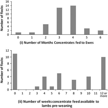
The results of the questionnaire, in relation to the concentrate feed used for ewe and pre-weaned lamb feeding, are shown in Figure 1. Rams were provided with concentrate feed during the month before mating in 34 out of the 39 flocks. The majority of flocks lambed during February and March. When asked to classify their overall farm, in terms of the stratified production levels, 64% classed their farms as a lowland system, 33% as an upland system and 3% as a hill system. The average flock size was 80 ewes, ranging from 12 to 220.
Concentrate feed use for (i) ewes and (ii) lambs.

Canonical correlation analysis
The first canonical variables were scaled so that the maximum coefficient in each case was ±1 resulting in the following equations:
P-value=+1.00×rams fed concentrates+0.002×number of weeks concentrate feed available to lambs pre-wean – 0.005×recorded ewe flock size−0.432×number of months ewes fed concentrates.
 $$\eqalignno{ Q\ {\rm value}=\,&{\minus}{\rm 1}.00{\times}{\rm UFD}{\minus}0.000{\rm 1}{\times}{\rm rainfall}{\minus}0.00{\rm 1 }\cr & {\times}{\rm sun\ hours} {\plus}0.{\rm 1}0{\rm 4}{\times}{\rm 21WT}{\plus}0.{\rm 235}{\times}{\rm UMD}\cr &{\plus}0.{\rm 249}{\times}{\rm temperature} $$
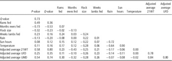
The corresponding canonical correlation between P and Q was 0.73. The first canonical P-variate represented the level of concentrate used in each system, with large, positive, values representing farms that fed their rams and lambs before mating and weaning, respectively. In addition, they had a lower flock size and the ewes were fed for fewer months throughout the year. Low, negative, values represented larger flocks, which fed their ewes for a longer period during the year. They did not, however, feed their rams or lambs before mating and weaning, respectively. The corresponding Q-variate, which utilised data available for all farms, had large, positive, values for farms with high performance averages for 21WT and UMD as well as high average temperatures and low average rainfall. The highest values along the scale were also associated with low UFD averages, as well as low rainfall and number of sun hours. Conversely, low values were associated with low temperatures and low performance averages for 21WT and UMD, as well as high average rainfall and UFD averages. Table 2 shows the correlations between all variables. Temperature and sun hours were highly correlated (r=0.90), which may explain the change in direction for sun hours when compared with the coefficient estimated in the canonical correlation analysis.
Correlations between all variables used in the canonical correlation analysis and the resulting P- and Q-variates

21WT=21-week-old weight; UMD=ultrasound muscle depth; UFD=ultrasound fat depth.
P-value and Q-value=values estimated using the P- and Q-variable equations, respectively, derived during the canonical correlation analyses.
Reaction norm analysis
The FE scale was then calculated using the weather and production information available for all 494 nationally recorded farms. By using the Q-value equation developed, the values estimated along the FE scale ranged from −1.40 to 2.66, with the average estimated across the population being 0.70. Overall, the scale went from low performance averages and poorer weather conditions to high performance averages and improved weather conditions. To illustrate, the average FE data for the 10 farms located at both extremes of the FE scale are shown in Table 3. The average values for 21WT, UMD and UFD were calculated using the original flock solutions (as estimated using the fixed effect model and that were used to calculate each Q-value) plus the average values across all levels of each fixed effect in the model.
Average descriptors for Texel sheep farms located at the 10 highest and 10 lowest points on the farm environment (FE) scale

21WT=21-week-old weight; UMD=ultrasound muscle depth; UFD=ultrasound fat depth.
Q-value=value estimated using the Q-variable equation derived during the canonical correlation analyses.
* Weather variables=overall 5-year annual averages (2005–2009).
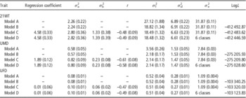
The variance component estimates obtained by models A, B, C and D are shown in Table 4. When models C and D were fitted, for each trait, two breeding values were produced, representing the intercept and slope of the reaction norm for each sire. The intercept value represented the average sire effect on each trait across all FEs. The slope represented the environmental sensitivity, or in other words the amount to which the sire effect was dependent on the FE value.
Estimates of fixed regression coefficients and variance components for intercept (σ 2 a), slope (σ 2 b), flock (σ 2 f), sire×flock interaction (σ 2 sf), error variance (σ e 2), log likelihood (LogL) and correlation (r) between intercept and slope from the reaction norm models for 21-week-old weight (21WT), ultrasound muscle depth (UMD) and ultrasound fat depth (UFD) (s.e. in parenthesis)

Model A=sire model with sire, flock and sire×flock fitted as random effects.
Model B=sire model, similar to model A, but with FE fitted as a covariate.
Model C=sire model, similar to model B but with sire, flock, sire×flock and sire×FE environment fitted as random effects.
Model D=sire model, similar to model C, but also accounting for heterogeneity of environmental variance.
6 classes=environmental classes a, b, c, d, e and f used for heterogeneity of environmental variance analysis.
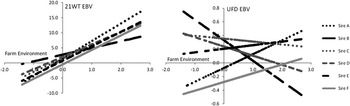
Based on the LR, model C, when compared with model B, significantly improved the fit of the model for 21WT and UFD (P<0.001), but not for UMD. Model D was found to be the best model for all traits (P<0.001). The results demonstrate that the inclusion of the sire×FE effect was significant for all traits, although only for UMD when heterogeneity of environmental variance was accounted for. The correlations between the intercept and slope, using model D, were all less than one and negative, 21WT (−0.49) and UMD (−0.58) and UFD (−0.49), implying the re-ranking of sires. Similar results were also obtained using model C. The reaction norms estimated for a sample of sires (the six sires with the most offspring in the data) in terms of their estimated breeding values (EBVs) for 21WT and UFD, are shown in Figure 2. The results for UMD were similar to those observed for 21WT. Overall, for 21WT and UMD, the EBVs of all sires improved as the FE improved. However, of the 5853 sires with UFD information, the EBVs of 61% of sires increased and 39% of sires decreased as the FE improved.
Reaction norms, for a sample of six sires (A to F), for 21-week-old weight (21WT) and ultrasound fat depth (UFD) estimated breeding values (EBVs) across the farm environment (FE) scale (using model B).

Heritability and correlation analysis
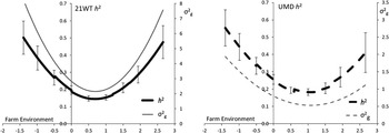
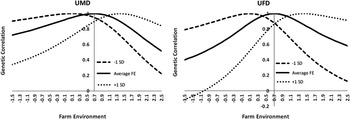
The heritabilities estimated using model B, for 21WT, UMD and UFD were 0.15 (±0.01), 0.19 (±0.02) and 0.17 (±0.02), respectively. When using model D, the range of heritability estimates for 21WT, UMD and UFD, along the FE scale were, 0.15 to 0.50, 0.18 to 0.55 and 0.15 to 0.63 for each trait, respectively. Similar estimates were observed when using model B also. The heritabilities estimated for 21WT and UMD, using model D, are shown in Figure 3. The heritability estimates for UFD followed a similar pattern as 21WT. The highest heritability estimates for 21WT and UFD were observed at each end of the FE scale and lowest at the mid-point, at approximately FE value 0.6. The heritability estimates for UMD followed a similar pattern, although the estimates at the high end were slightly lower than those estimated at the low end. It should also be noted that the largest standard errors, for all traits, were associated with heritability estimates at both extremes of the FE scale. The genetic variances estimated followed a similar pattern as the heritability estimates (Figure 3). The genetic correlations estimated across the FE scale are shown in Figure 4. The correlations estimated ranged from −0.42 to 1 for 21WT, −0.22 to 1 for UMD and −0.51 to 1 for UFD. The correlations shown in Figure 4, for UMD and UFD, are estimated for flocks with an average Q-value in the population (0.7) as well as those ±1 standard deviation (s.d.) from the average. Similarly, those in Figure 5 for UMD and UFD demonstrate how the correlations change between all environments. The results for 21WT were similar to those observed for UMD and UFD.
Heritability (h 2 ) and genetic variance (σ 2 g) estimates, for 21-week-old weight (21WT), ultrasound muscle depth (UMD) as functions of the farm environment (FE) scale (using model D).

Genetic correlations estimated for ultrasound muscle depth (UMD) and ultrasound fat depth (UFD) across the farm environment (FE) scale. Graphs shown are between flocks with environment values of −1 s.d. from the average, average and +1 s.d. from the average, respectively, and all other environments along the FE scale.

Genetic correlations estimated across the farm environment (FE) scale between pairs of FEs (FE1 and FE2) for ultrasound muscle depth (UMD) and ultrasound fat depth (UFD).

Spearman’s rank correlations were also calculated using the breeding values estimated for all 5938 sires represented in the data, between environments ±0.5, ±1.0 and ±1.5 s.d. from the average Q-value. The results observed for 21WT, between −0.5 and +0.5; −1.0 and +1.0; and −1.5 and +1.5 s.d. from the average were 0.97, 0.90 and 0.79, respectively. The correlations estimated UMD and UFD between −0.5 and +0.5, −1.0 and +1.0 and −1.5 and +1.5 s.d. from the average were 0.99, 0.96 and 0.94 and 0.96, 0.86 and 0.72, respectively.
Discussion
Defining FE
The canonical correlation analysis used in the present study provided an opportunity to relate fine scale information gathered from a sample of farms, with information available from farms at a national level. The concentrate feed-related variables obtained from the farm survey were selected for further analysis in order to improve our knowledge of the effects that different feeding regimes may have. When using canonical correlation analysis it is important to be aware of the sensitivity of the method with regards to any changes to the variables used (Hair et al., Reference Hair, Tatham, Anderson and Black2006). Although the results should be treated with a certain level of caution, due to the fact that the analysis was based on 40 randomly selected farms, they are still worthy of consideration. The canonical correlation estimated was reasonably high (0.73), therefore suggesting that the first canonical Q-variable was a useful measure of system input (in terms of the use of supplementary feed), and thus FE overall. The correlation estimated by Haskell et al. (Reference Haskell, Brotherstone, Lawrence and White2007), when defining dairy farm FE, using a similar method, was 0.62. An interpretation of the first Q-variable suggests, in terms of the production averages, that high FE values were associated with high performance averages for 21WT and UMD, and low averages for UFD. The Terminal Sire Index, within which the majority of Texel breeders record, has weightings on each of these traits in order to improve 21WT and UMD while reducing any associated rise in UFD (Simm and Dingwall, Reference Simm and Dingwall1989; Macfarlane and Simm, Reference Macfarlane and Simm2007). Therefore, the FE scale developed is a relatively good reflection of the overall aim of the breeding index. Similarly, the direction of the weather variables, in general, suggests that the highest FE values are associated with higher average temperatures and lower rainfall. This would agree with the general assumption that areas with better weather conditions have improved environments in terms of aspects such as pasture availability and quality.
The first canonical P-variable, using data from the survey farms, provided an interesting result when compared with the corresponding canonical Q-variable. Farms with a high P-value were associated with a higher use of ram and pre-weaned lamb concentrate feeding, but less so with ewe feeding and the overall flock size. The majority of flocks fed their rams during the month before mating. However, there was quite a range in the number of weeks before weaning, during which lambs had access to supplementary feed. The increased use of concentrate feed, particularly for pre-weaned lambs, is likely to have helped improve the production averages. However, when considered alongside the weather variables, it would seem that these farms already had a favourable FE and therefore these farms have chosen to try and improve the environment further by allowing their lambs access to feed before they are weaned.
Farms with a lower P-value fed their ewes for a longer period during the year than those at the other end of the scale. This could again be related to the weather variables. In areas with lower average temperatures and higher rainfall, the increased use of feeding could be used to help maintain the condition of the ewe throughout pregnancy, and possibly post-pregnancy. This could be because the ewes have been kept outside in potentially poorer conditions where grass growth can be limited for a greater number of months. Alternatively, in order to remove the effects of the poorer weather conditions, they may have been housed for a longer period of time before and during lambing. Whatever the system used, both rely on the use of substantial amounts of supplementary feed for the ewes. The emphasis has therefore moved from improving lamb performance further, to perhaps better maintaining the ewe throughout pregnancy. With the variation over the past few years in the price of concentrate feed, both nationally and worldwide, if feed prices increase, while the price of lamb does not increase at a similar rate, farmers may decide to make adjustments to their management system. Should they cut back on the level of feed that they provide to their flocks, by using the scale described in the present study, farmers could potentially identify sires best suited to which ever system they choose to pursue.
Although the initial aim of the analysis was to identify a way of measuring the level of concentrate feed use, the resulting FE scale, as estimated using the first canonical Q-value, was not dissimilar to a production level-type scale. Similar scales have been used in studies such as those by Strandberg et al. (Reference Strandberg, Brotherstone, Wall and Coffey2009), who, in addition to using the FE scale developed by Haskell et al. (Reference Haskell, Brotherstone, Lawrence and White2007), also used herd averages for production and fertility-related descriptors to define environments. Kolmodin et al. (Reference Kolmodin, Strandberg, Madsen, Jensen and Jorjani2002), defined environments as the deviation from the overall herd-year averages of protein production (production environment) and days open (fertility environment). Studies using sheep, such as Pollot and Greeff (Reference Pollot and Greeff2004), defined Merino production environments using the average value of each trait analysed, for each contemporary group identified. Similar methods have also been used by Santana et al. (Reference Santana, Bignardi, Eler, Cardoso and Ferraz2013b) when studying Santa Ines sheep in Brazil.
However, it should be noted that before any scale can be introduced to the industry, further investigation would be required in order to identify an appropriate method by which the farmers could use this information. The scale used in the present study uses adjusted performance averages for a number of traits, therefore it may be more appropriate for the farmers to receive information with regards to a pre-calculated FE score when they receive their flock genetic evaluation data. It should also be noted that the scale discussed here was for a specific breed and specific lamb traits. It may be that the scale would be different if other breeds or traits were involved.
Reaction norm analysis
The reaction norms estimated for each trait suggest G×E was evident, in terms of both re-ranking and scaling. The sensitivities estimated, as represented by the slope value for each sire reaction norm, indicated that all sires represented in the dataset increased their performance, for 21WT and UMD, as the FE improved. When the overall regression coefficient was removed, there was a mix of positive and negative values indicating variation in the level of improvement across the scale. In other words, some improved at a quicker rate than others. However, for UFD, the EBVs of some sires increased as the FE improved while others decreased as the FE improved. Overall, the range of slope gradients observed for each sire reaction norm indicated the presence of both scaling and re-ranking. It should be noted though that a number of sires had sensitivities close to, or equal to, zero, indicating that there was very little variation in their performance across environments and they were therefore not influenced as much by changes in feeding regimes. Similar examples of scaling and re-ranking were observed by both Pollot and Greeff (Reference Pollot and Greeff2004) and Santana et al. (Reference Santana, Bignardi, Eler, Cardoso and Ferraz2013b), when using random regression models to investigate a number of sheep performance traits including faecal egg counts, wool, body and growth characteristics. Overall, as suggested by Haskell et al. (Reference Haskell, Brotherstone, Lawrence and White2007), the presence of environmental sensitivity provides an opportunity for farmers to choose sires based on the FE of their farm.
When heterogeneous residual variances were investigated, their inclusion significantly improved the fit of the overall random regression model for all traits. Similar results were also observed by Pollot and Greeff (Reference Pollot and Greeff2004), Cardoso and Tempelman (Reference Cardoso and Tempelman2012) and Santana et al. (Reference Santana, Bignardi, Eler, Cardoso and Ferraz2013b). Strandberg (Reference Strandberg2006) comments that this is not unexpected, particularly when using sire models. The six environmental classes (a to f) used for the analyses were kept consistent across the traits, and were selected based on the different sections of the FE scale, representing low, average and high environments. Although these classes provided significant improvements to the fit of the model, it may be that the fit could be improved further by adjusting the classes and using different classes for different traits. Nonetheless, the results presented here highlight that it may be beneficial for any similar analyses in the future to account for such heterogeneous variances.
Heritability of traits across different environments
When using environment scales based on production levels, such as those used by Kolmodin et al. (Reference Kolmodin, Strandberg, Madsen, Jensen and Jorjani2002) and Strandberg et al. (Reference Strandberg, Kolmodin, Madsen, Jensen and Jorjani2000), the heritabilities estimated often increased as the environment improved. Heritabilities previously estimated, using data available for Texel lambs in the United Kingdom, for 21WT, UMD and UFD were 0.38, 0.29 and 0.38, respectively (Jones et al., Reference Jones, Lewis, Young and Simm2004). When the heritabilities of the three traits were estimated across the FE scale, in the present study, the highest values were estimated at the extremes of the scale for 21WT and UFD. However, it should be noted that these estimates were also associated with the highest standard errors therefore they should be treated with caution. The lowest values, and lowest standard errors, for these traits were estimated at the mid-point of the scale, possibly due to the distribution of the farms on the scale. These results are similar to those estimated by Pollot and Greeff (Reference Pollot and Greeff2004) for faecal egg count across environments. The estimates for UMD were slightly different than those for 21WT and UFD. The highest values estimated at the low end for the scale and the lowest values slightly above the mid-point, but again the standard errors were larger at the extremes of the FE scale and smaller nearer the mid-point.
The heritability estimates for 21WT, UMD and UFD at the low end of the FE scale (poorer FE environment in terms of production and weather), indicated that the genetic variation for these traits was high. This would suggest that some rams have the ability to produce lambs with high 21WT, UMD and UFD values even when the environment is classed as poorer. Similarly, and perhaps somewhat more expected, at the higher end of the FE scale, the heritability estimates increased as the environment improved. The rate of increase was the highest for UFD, followed by 21WT, suggesting that the genetic control over these traits was affected more by the improvement in environment than UMD. The observed rate of increase should be treated with some caution due to the increased size of the standard errors associated with these estimates. At the mid-point of the scale, the animals were generally more similar in their genetic control of each trait. The lowest heritability values for UMD were estimated just above the mid-point of the scale. This, along with the fact that the UMD heritability estimates were the highest overall at the poorer end of the scale, indicates that improvements in this trait can also be made when environmental conditions are not so favourable.
In terms of the different feeding levels, the results suggest that by increasing the amount of feed available to lambs, although improvements will be found with regards to all traits, the rate of genetic progress associated with UFD will be the greatest. This may prove costly if carcasses become over-fat and result in a financial penalty to the farmer. At the lower end of the FE scale, if the lambs are fed less feed, but the ewes are fed more, the rate of genetic progress of all three traits will also improve at a similar rate.
Genetic correlations between farm environments
A wide range of genetic correlations were estimated within each trait, between pairs of environments across the FE scale. The results suggest that there would be less G×E evident, in terms sires ranking, if the environmental conditions of the two environments were similar. For example, flocks with below average Q-values on the FE scale were relatively highly correlated with similar flocks located at that end of the FE scale and similarly, flocks with above average Q-values were more highly correlated with other flocks at the top end of the FE scale. However, as the environments become more divergent (e.g. the lowest points of the FE scale and the highest points on the FE scale) the genetic and Spearman’s rank correlations fell. Sires suitable for flocks at the lower end of the FE scale are therefore not necessarily as suitable for those at the higher end of the FE scale and this further emphasises that G×E is evident in the population. These results were similar to those reported by Santana et al. (Reference Santana, Bignardi, Eler, Cardoso and Ferraz2013b) for the BW of Santa Ines sheep at 180 days of age as well as Cardoso and Tempelman (Reference Cardoso and Tempelman2012) for post-weaning weight gain of Angus cattle.
Accounting for G×E in genetic evaluations
Overall, the use of reaction norm analyses provide an opportunity for future genetic evaluations to take into account any interactions that may be present between genotypes and environments. The reduced requirement for each individual environment to be genetically linked, such as those required when using the multi-trait method and groups of environments, potentially allows the prediction of an animal’s performance across a greater number of environments. Providing a suitable ‘measure of environment’ can be agreed, the method can allow the prediction of unique rankings for each level of environment.
The method presented in the current study combined fine-level detail, with particular emphasis on the use of concentrate feed, with information available nationally for all flocks that are members of Signet Sheepbreeder programme. By using the environment scale developed, G×E was observed for all Texel lamb traits investigated, both in terms of re-ranking and scaling. The variation in heritability estimates across different environments, as well as the range of genetic correlations estimated between environments, all need consideration in future selection programmes. Mulder et al. (Reference Mulder, Veerkamp, Ducro, van Arendonk and Bijma2006) recommended, while investigating the presence of G×E in dairy cattle, that when genetic correlations between environments were below 0.61, different breeding programmes should be used. However, whether this specific value is relevant to the sheep breeding situation of the present study, or economically viable, would be worthy of further investigation. It may also be useful to investigate if the FE scale developed in this study is applicable to other traits and breeds, or if another way of quantifying FE should be considered.
Conclusions
The techniques and approaches used in this study have proven to be useful in defining sheep FEs and have the potential to be adopted across the globe in relation to different farming systems. Although the environment scale identified in the current study may perhaps be more relevant to terminal sire breeds and traits, there is no reason why variables better suited to other breed types, such as hill breeds for example, cannot be identified and used in a similar manner. The range of sire sensitivities estimated across the environment scale, using the reaction norm methods, confirmed the presence of genetic variability, as both ‘plastic’ and ‘robust’ genotypes were observed in the population. The ability to identify differences in sensitivity allows farmers to select animals best suited to specific environments as well those that will perform consistently across a range of environments. The variation in heritability and correlation estimates also suggests that the rate genetic progress will vary depending on the environment. Overall, the results from this study indicate that in order to improve genetic gain and flock efficiency, future genetic evaluations would benefit by accounting for the G×E observed.
Acknowledgements
The author wishes to acknowledge EBLEX, HCC and QMS for funding this research. Many thanks also to the farmers who responded to the questionnaire, Ian White (University of Edinburgh) and Sebastian Mucha (SRUC) for their advice in regards to the data analysis and Sam Boon (Signet Breeding Services) and Kirsty Moore (EGENES) for their help with providing the data.