1 Introduction
Gravity currents, also known as buoyancy or density currents, occur whenever fluid of one density flows primarily horizontally into fluid of a different density (Huppert Reference Huppert2006). The density difference between the fluids, which provides the driving force behind such flows, may be attributed to a number of factors, including temperature differentials, dissolved materials and suspended sediments. The readers are referred to Allen (Reference Allen1985) and Simpson (Reference Simpson1997) for a comprehensive introduction to this topic in a variety of geophysical and industrial situations.
In the literature, a large number of laboratory experiments have been performed for such flows in a channel and the flows are confined between parallel lateral walls. A barrier is typically placed inside the channel, where two sides of the barrier are filled with fluids of different densities. Removal of the barrier then sets the two fluids into motion. This type of experiment, i.e. lock-exchange flow, serves as a model for studies of many geophysical and industrial flows and has drawn the most attention. If viscous effects due to the lateral walls can be ignored, the gravity currents produced in such an experimental set-up propagate as a statistically two-dimensional flow, also known as planar gravity currents. The dynamics of planar gravity currents is comparatively well understood, with the help of laboratory experiments (e.g. Huppert & Simpson Reference Huppert and Simpson1980; Shin, Dalziel & Linden Reference Shin, Dalziel and Linden2004; Marino, Thomas & Linden Reference Marino, Thomas and Linden2005; La Rocca et al. Reference La Rocca, Adduce, Sciortino and Pinzon2008; Adduce, Sciortino & Proietti Reference Adduce, Sciortino and Proietti2012; Dai Reference Dai2013, Reference Dai2014; Lombardi et al. Reference Lombardi, Adduce, Sciortino and La Rocca2015; Ottolenghi et al. Reference Ottolenghi, Adduce, Inghilesi, Armenio and Roman2016a ,Reference Ottolenghi, Adduce, Inghilesi, Roman and Armenio b ) and numerical simulations (e.g. Härtel, Meiburg & Necker Reference Härtel, Meiburg and Necker2000b ; Cantero et al. Reference Cantero, Lee, Balachandar and Garcia2007b ; La Rocca et al. Reference La Rocca, Adduce, Lombardi, Sciortino and Hinkermann2012a ,Reference La Rocca, Adduce, Sciortino, Bateman and Boniforti b ; Dai Reference Dai2015; Dai & Huang Reference Dai and Huang2016). The planar gravity currents produced by lock exchange may go through three distinct phases of spreading in sequence, namely the slumping, inertial and viscous phases, and the spatio-temporal evolution of planar gravity currents is well documented in these references, to mention but a few.
There are a number of geophysical and industrial situations in which the gravity currents are not constrained by lateral walls but are allowed to spread out radially over the entire horizontal plane. In such situations, the gravity currents propagate as a statistically axisymmetric flow, also known as cylindrical gravity currents. Experimental and computational investigations of cylindrical gravity currents are comparatively limited (Huppert & Simpson Reference Huppert and Simpson1980; Bonnecaze et al.
Reference Bonnecaze, Hallworth, Huppert and Lister1995; Alahyari & Longmire Reference Alahyari and Longmire1996; Hallworth et al.
Reference Hallworth, Huppert, Phillips and Sparks1996; Huq Reference Huq1996; Ungarish & Zemach Reference Ungarish and Zemach2005; Patterson et al.
Reference Patterson, Simpson, Dalziel and Van Heijst2006; Ross, Dalziel & Linden Reference Ross, Dalziel and Linden2006; Cantero, Balachandar & Garcia Reference Cantero, Balachandar and Garcia2007a
; Ungarish Reference Ungarish2007; Ungarish & Huppert Reference Ungarish and Huppert2008; Ungarish Reference Ungarish2010). For cylindrical gravity currents, as demonstrated by Ungarish (Reference Ungarish2007), the propagation is first dominated by the inertial–buoyancy balance, during which slumping and then self-similar stages occur; then a transition to the viscous–buoyancy balance phase occurs, in which a different self-similar motion develops. With the help of high-resolution simulations, Cantero et al. (Reference Cantero, Balachandar and Garcia2007a
) observed that the Kelvin–Helmholtz vortices occur only during the slumping phase and the wavelength of the lobes grows, while the number of lobes around the circumference is maintained, as the flow spreads. For non-rotating cylindrical gravity currents, the radius of the current
 $\tilde{R}$
as a function of time
 $\tilde{t}$
follows
 $$\begin{eqnarray}\displaystyle \tilde{R}\approx 1.16(\tilde{g}_{0}^{\prime }\tilde{V}_{0})^{1/4}\tilde{t}^{1/2}\quad \text{or}\quad \frac{\tilde{R}}{\tilde{R}_{0}}\approx 1.16\unicode[STIX]{x03C0}^{1/4}\frac{\tilde{g}_{0}^{\prime 1/4}\tilde{H}^{1/4}}{\tilde{R}_{0}^{1/2}}\tilde{t}^{1/2}, & & \displaystyle\end{eqnarray}$$
for the self-similar motion in the inertial–buoyancy balance phase and
 $$\begin{eqnarray}\displaystyle \tilde{R}\approx 0.779(\tilde{g}_{0}^{\prime }\tilde{V}_{0}^{3}/\unicode[STIX]{x1D708})^{1/8}\tilde{t}^{1/8}, & & \displaystyle\end{eqnarray}$$
for the viscous–buoyancy balance phase (Huppert & Simpson Reference Huppert and Simpson1980; Huppert Reference Huppert1982), where
 $\tilde{g}_{0}^{\prime }$
is the reduced gravity,
 $\tilde{V}_{0}=\unicode[STIX]{x03C0}\tilde{R}_{0}^{2}\tilde{H}$
is the volume of heavy fluid in the cylindrical lock,
 $\tilde{R}_{0}$
is the radius of the cylindrical lock,
 $\tilde{H}$
is the depth of heavy fluid and
 $\unicode[STIX]{x1D708}$
is the kinematic viscosity of the heavy fluid.
In other large-scale geophysical situations, the influence of the Coriolis force due to the Earth’s rotation will definitely play a major role in the propagation of gravity currents (Griffiths Reference Griffiths1986). A notable example, related to the present investigation, is the oceanographic structure called a warm or cold core ‘ring’, ‘vortex’ or ‘lens’ (Saunders Reference Saunders1973; Csanady Reference Csanady1979; Flierl Reference Flierl1979; Killworth Reference Killworth1992; Rubino & Brandt Reference Rubino and Brandt2003; Stegner, Bouruet-Aubertot & Pichon Reference Stegner, Bouruet-Aubertot and Pichon2004; Sutyrin Reference Sutyrin2006). A ‘ring’ in the ocean is a flow structure associated with an isolated mass of anomalous water, significantly warmer or colder, saltier or fresher than its surroundings. It is known that unstable meanders of the Gulf Stream and of the Kuroshio can inject a parcel of water of one density into surroundings of a different density, and the parcel becomes an isolated ‘ring’ when a geostrophic equilibrium is established.
In the laboratory, such flows are modelled by releasing cylindrical gravity currents on a rotating turntable. For cylindrical gravity currents generated from a full-depth cylindrical lock release in a rotating system, the ratio of Coriolis to inertia forces, i.e.
 $$\begin{eqnarray}\displaystyle {\mathcal{C}}=\frac{\tilde{\unicode[STIX]{x1D6FA}}\tilde{R}_{0}}{\sqrt{\tilde{g}_{0}^{\prime }\tilde{H}}}, & & \displaystyle\end{eqnarray}$$
is the most important parameter, where
 $\tilde{\unicode[STIX]{x1D6FA}}$
is the angular velocity of the rotating system,
 $\tilde{R}_{0}$
is the radius of the cylindrical lock,
 $\tilde{H}$
is the depth of fluid and
 $\tilde{g}_{0}^{\prime }$
is the reduced gravity. Here the ratio of Coriolis to inertia forces is related to the Rossby number, i.e.
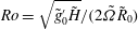 $Ro=\sqrt{\tilde{g}_{0}^{\prime }\tilde{H}}/(2\tilde{\unicode[STIX]{x1D6FA}}\tilde{R}_{0})$
, via
 $Ro=1/(2{\mathcal{C}})$
and is also related to the ratio of the radius of the cylindrical lock,
 $\tilde{R}_{0}$
, to the deformation radius,
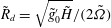 $\tilde{R}_{d}=\sqrt{\tilde{g}_{0}^{\prime }\tilde{H}}/(2\tilde{\unicode[STIX]{x1D6FA}})$
, via
 ${\mathcal{C}}=\tilde{R}_{0}/(2\tilde{R}_{d})$
. In other words, the ratio of Coriolis to inertia forces is related to the Burger number, i.e.
 $Bu=\tilde{R}_{d}^{2}/\tilde{R}_{0}^{2}$
, via
 $Bu=1/(4{\mathcal{C}}^{2})$
(e.g. Rubino & Brandt Reference Rubino and Brandt2003; Stegner et al.
Reference Stegner, Bouruet-Aubertot and Pichon2004). In the experiments of Saunders (Reference Saunders1973), the heavy fluid is placed inside the cylindrical lock to the same depth of and surrounded by light ambient fluid so the vortex is formed on the bottom once the lock is removed. Saunders (Reference Saunders1973) reported that the ‘bottom vortex’ is stable when
 ${\mathcal{C}}\leqslant 0.37$
. Under the condition when
 ${\mathcal{C}}>0.37$
, the ‘bottom vortex’ exhibits unstable azimuthal waves, which grow to an amplitude such that they become cutoff distinct circulations, i.e. vortex splitting occurs. The number of amplifying waves and hence vortices is dependent solely on the ratio of Coriolis to inertia forces. It was also confirmed by Saunders (Reference Saunders1973) that the aspect ratio of the cylindrical lock,
 $\tilde{R}_{0}\tilde{H}^{-1}$
, has an unnoticed influence on the results. In contrast, Griffiths & Linden (Reference Griffiths and Linden1981) performed experiments in which fluid inside the cylindrical lock is less dense than the environment so the vortex is formed at the free surface rather than on the bottom. However, the ‘surface vortex’ is always unstable, even when
 ${\mathcal{C}}\leqslant 0.37$
. Griffiths & Linden (Reference Griffiths and Linden1981) attributed the stability of the ‘bottom vortex’ to the action of the viscous Ekman layer at the bottom.
For stable cylindrical gravity currents in a rotating system, i.e. ‘bottom vortex’ when
 ${\mathcal{C}}\leqslant 0.37$
, Ungarish & Huppert (Reference Ungarish and Huppert1998) and Hallworth, Huppert & Ungarish (Reference Hallworth, Huppert and Ungarish2001) investigated the problem using laboratory experiments, shallow-water formulation and finite-difference numerical solutions of the axisymmetric Navier–Stokes equations. It was found that Coriolis effects are negligible during the initial one-tenth of a revolution of the system following the release of the heavy fluid. A major feature of rotating cylindrical gravity currents was the attainment of a maximum radius of propagation. The maximum radius of rotating cylindrical gravity currents, as a function of the ratio of Coriolis to inertia forces, follows
 $$\begin{eqnarray}\displaystyle \tilde{R}_{max}\approx 1.6{\mathcal{C}}^{-1/2}\tilde{R}_{0}, & & \displaystyle\end{eqnarray}$$
for
 ${\mathcal{C}}\ll 1$
(Ungarish & Huppert Reference Ungarish and Huppert1999). A maximum radius of propagation is reached in less than half of a revolution of the system. Thereafter a contraction–relaxation motion in the body of heavy fluid and a regular series of outwardly propagating pulses were observed. These features in rotating cylindrical gravity currents have no counterparts in non-rotating situations. However, it should be recognized that the rotating experiments are expensive, time consuming and there exist technical difficulties in obtaining detailed information in space and time about the density and velocity fields. The shallow-water formulation can correctly capture the pulse period and several other dynamical behaviours if
 ${\mathcal{C}}$
is not too small, e.g.
 ${\mathcal{C}}\approx 3.54$
in Rubino & Brandt (Reference Rubino and Brandt2003). For
 ${\mathcal{C}}\ll 1$
, the shallow-water formulation for rotating cylindrical gravity currents predicts quite well the gravity current shape development, the change from positive to negative radial velocity during propagation, the time of attainment of the maximum radius, the development of the retrograde azimuthal velocity in the current and more (Ungarish & Huppert Reference Ungarish and Huppert1998; Hallworth et al.
Reference Hallworth, Huppert and Ungarish2001). However, the shallow-water formulation does not repeatedly capture the contraction–relaxation motion for
 ${\mathcal{C}}\ll 1$
, nor does it provide detailed three-dimensional information and small-scale structures in the flow field.
Numerical solutions of the axisymmetric Navier–Stokes equations capture more details of the flow field but, unfortunately, the contraction–relaxation motion cannot be faithfully reproduced in this manner either. Furthermore, it should be kept in mind that axisymmetric solutions, which ignore the variations in the azimuthal direction, are incompatible with some of the complex features in real cylindrical gravity currents, e.g. the lobe-and-cleft structure. The variations in the flow field in the azimuthal direction, along with those in other directions, must be captured by means of three-dimensional high-resolution simulations without imposed axisymmetry conditions.
This study aims at investigating the dynamical processes in the formation of stable cylindrical gravity currents, by a full-depth lock release in a rotating system. Our focus is on the situation when the ratio of Coriolis to inertia forces is not large and, specifically,
 ${\mathcal{C}}=0.1,0.2,0.3$
are considered in this study. Since our intent is to provide detailed information in space and time about the density and velocity fields in rotating cylindrical gravity currents, the investigation is conducted by means of three-dimensional high-resolution simulations of the incompressible variable-density Navier–Stokes equations with the Coriolis term. With the detailed information in the flow field, qualitative and quantitative measures for the dynamical processes in the formation of stable rotating cylindrical gravity currents are now shown more clearly for the first time. In § 2, we describe the formulation of the problem and the numerical procedure. The qualitative and quantitative results are presented in § 3. Finally, conclusions are drawn in § 4.
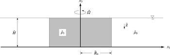
Sketch of the initial condition for a cylindrical gravity current, produced by a full-depth lock release, in a rotating system. At
 $t=0$
, heavy fluid of density
 $\tilde{\unicode[STIX]{x1D70C}}_{1}$
is confined in the cylindrical lock, of which the radius is
 $\tilde{R}_{0}=\tilde{H}$
. Outside the cylindrical lock is the light ambient fluid of density
 $\tilde{\unicode[STIX]{x1D70C}}_{0}$
. Before the heavy fluid is released from the lock, the system is in solid-body rotation with constant angular velocity
 $\tilde{\unicode[STIX]{x1D6FA}}$
about the vertical axis
 $x_{3}$
. Removal of the cylindrical lock sets the quiescent fluid, observed in the rotating frame, into motion.

2 Formulation
Figure 1 gives a sketch of the configuration for simulations of cylindrical gravity currents produced by a full-depth lock release in a rotating system. The heavy fluid of density
 $\tilde{\unicode[STIX]{x1D70C}}_{1}$
is confined in the cylindrical lock region of radius
 $\tilde{R}_{0}$
and filled to the same depth
 $\tilde{H}$
as the light ambient fluid outside the cylindrical lock region. The density of the light ambient fluid is
 $\tilde{\unicode[STIX]{x1D70C}}_{0}$
. Here the radius of the cylindrical lock is chosen the same as the depth of fluid, i.e.
 $\tilde{R}_{0}=\tilde{H}$
. Before the release of heavy fluid, the system of heavy fluid and light ambient fluid is in solid-body rotation with constant angular velocity
 $\tilde{\unicode[STIX]{x1D6FA}}$
about the vertical axis
 $x_{3}$
with a gravitational acceleration in the antiparallel direction of
 $x_{3}$
. Here we adopt the Boussinesq approximation, in that the density difference, (
 $\tilde{\unicode[STIX]{x1D70C}}_{1}-\tilde{\unicode[STIX]{x1D70C}}_{0}$
), is assumed sufficiently small compared with the reference density
 $\tilde{\unicode[STIX]{x1D70C}}_{0}$
such that the influence of density variations is retained only in the buoyancy term but neglected in the inertia and diffusion terms. Consequently, the governing equations take the form, using tensor notation,
 $$\begin{eqnarray}\displaystyle & \displaystyle \frac{\unicode[STIX]{x2202}u_{k}}{\unicode[STIX]{x2202}x_{k}}=0, & \displaystyle\end{eqnarray}$$
 $$\begin{eqnarray}\displaystyle & \displaystyle \frac{\unicode[STIX]{x2202}u_{i}}{\unicode[STIX]{x2202}t}+\frac{\unicode[STIX]{x2202}(u_{i}u_{k})}{\unicode[STIX]{x2202}x_{k}}=\unicode[STIX]{x1D70C}e_{i}^{g}-\frac{\unicode[STIX]{x2202}p}{\unicode[STIX]{x2202}x_{i}}-2{\mathcal{C}}R_{0}^{-1}\unicode[STIX]{x1D700}_{ijk}e_{j}^{\unicode[STIX]{x1D6FA}}u_{k}+\frac{1}{Re}\frac{\unicode[STIX]{x2202}^{2}u_{i}}{\unicode[STIX]{x2202}x_{k}\unicode[STIX]{x2202}x_{k}}, & \displaystyle\end{eqnarray}$$
 $$\begin{eqnarray}\displaystyle & \displaystyle \frac{\unicode[STIX]{x2202}\unicode[STIX]{x1D70C}}{\unicode[STIX]{x2202}t}+\frac{\unicode[STIX]{x2202}(\unicode[STIX]{x1D70C}u_{k})}{\unicode[STIX]{x2202}x_{k}}=\frac{1}{Pe}\frac{\unicode[STIX]{x2202}^{2}\unicode[STIX]{x1D70C}}{\unicode[STIX]{x2202}x_{k}\unicode[STIX]{x2202}x_{k}}. & \displaystyle\end{eqnarray}$$
 $u_{i}$
denotes the velocity,
 $\unicode[STIX]{x1D70C}$
the density,
 $e_{i}^{g}$
the unit vector in the direction of gravity,
 $e_{j}^{\unicode[STIX]{x1D6FA}}$
the unit vector in the direction of rotation,
 $p$
the pressure and
 $\unicode[STIX]{x1D700}_{ijk}$
the Levi-Civita symbol. Please note that the centrifugal term, which can be written as the gradient of a scalar, is combined with the pressure term in (2.2) without loss of generality. The set of (2.1)–(2.3) is made dimensionless by the lock height,
 $\tilde{H}$
, as the length scale and the buoyancy velocity
 $$\begin{eqnarray}\displaystyle \tilde{u} _{b}=\sqrt{\tilde{g}_{0}^{\prime }\tilde{H}}\quad \text{with }\tilde{g}_{0}^{\prime }=\tilde{g}\frac{\tilde{\unicode[STIX]{x1D70C}}_{1}-\tilde{\unicode[STIX]{x1D70C}}_{0}}{\tilde{\unicode[STIX]{x1D70C}}_{0}}, & & \displaystyle\end{eqnarray}$$
as the velocity scale. Since the radius of the cylindrical lock is set to be the same as the depth of fluid, the dimensionless radius of the lock is unity, i.e.
 $R_{0}=1$
. The dimensionless density, i.e. the concentration of fluid mixture, is given by
 $$\begin{eqnarray}\displaystyle \unicode[STIX]{x1D70C}=\frac{\tilde{\unicode[STIX]{x1D70C}}-\tilde{\unicode[STIX]{x1D70C}}_{0}}{\tilde{\unicode[STIX]{x1D70C}}_{1}-\tilde{\unicode[STIX]{x1D70C}}_{0}}. & & \displaystyle\end{eqnarray}$$
The relevant dimensionless parameters are the ratio of Coriolis to inertia forces, defined by (1.3), the Reynolds number
 $Re$
and the Péclet number
 $Pe$
, defined by
 $$\begin{eqnarray}\displaystyle Re=\frac{\tilde{u} _{b}\tilde{H}}{\tilde{\unicode[STIX]{x1D708}}}\quad \text{and}\quad Pe=\frac{\tilde{u} _{b}\tilde{H}}{\tilde{\unicode[STIX]{x1D705}}}, & & \displaystyle\end{eqnarray}$$
respectively. The two fluids are assumed to have identical kinematic viscosities
 $\tilde{\unicode[STIX]{x1D708}}$
and diffusion coefficients
 $\tilde{\unicode[STIX]{x1D705}}$
. They are related by the Schmidt number
 $$\begin{eqnarray}\displaystyle Sc=\frac{\tilde{\unicode[STIX]{x1D708}}}{\tilde{\unicode[STIX]{x1D705}}}, & & \displaystyle\end{eqnarray}$$
which represents the ratio of the kinematic viscosity to molecular diffusivity. Typically in saline experiments,
 $Sc\approx 700$
, but it has been observed by many researchers (e.g. Härtel et al.
Reference Härtel, Meiburg and Necker2000b
; Necker et al.
Reference Necker, Härtel, Kleiser and Meiburg2005; Cantero et al.
Reference Cantero, Lee, Balachandar and Garcia2007b
; Bonometti & Balachandar Reference Bonometti and Balachandar2008) that the influence of Schmidt number on the dynamics of the gravity current is weak as long as
 $Sc\approx O(1)$
or larger. Therefore we follow suit here and employ
 $Sc=1$
in the simulations. The Ekman number, which expresses the ratio of viscous to Coriolis forces, is defined as
 $$\begin{eqnarray}\displaystyle E=\frac{\tilde{\unicode[STIX]{x1D708}}}{\tilde{\unicode[STIX]{x1D6FA}}\tilde{H}^{2}}, & & \displaystyle\end{eqnarray}$$
which can also be expressed in terms of the previous parameters by
 $E=R_{0}({\mathcal{C}}Re)^{-1}$
.
The set of equations in the velocity–pressure formulation is solved with resolution
 $N_{x_{1}}\times N_{x_{2}}\times N_{x_{3}}$
. The length is non-dimensionalized by the lock height,
 $\tilde{H}$
, and the flow domain is
 $L_{x_{1}}\times L_{x_{2}}\times L_{x_{3}}=15\times 15\times 1$
in order to allow unhindered development of the rotating cylindrical gravity currents. Fourier expansion with periodic boundary condition is employed in the horizontal directions, i.e.
 $x_{1}$
and
 $x_{2}$
. Chebyshev expansion with Gauss–Lobatto quadrature points is employed in the wall-normal direction, i.e.
 $x_{3}$
. The Gauss–Lobatto quadrature points provide a straightforward implementation of boundary conditions and have high resolution near the walls. As argued by Hallworth et al. (Reference Hallworth, Huppert and Ungarish2001), the free surface deviates from the horizontal but neglecting such a deviation is justified for small density contrast between heavy and light ambient fluids and for small ratio of Coriolis to inertia forces. Following previous experimental and numerical investigations of rotating cylindrical gravity currents (Ungarish & Huppert Reference Ungarish and Huppert1998; Hallworth et al.
Reference Hallworth, Huppert and Ungarish2001), we employ no-slip and no-stress conditions for the velocity field at the bottom and top boundaries, respectively, and a no-flux condition for the density field at the bottom and top boundaries. The influence of periodic boundary condition in the horizontal directions will not be discussed here since previous computational investigations have shown that the interaction of the gravity currents with the boundary becomes important only when the front reaches within one depth scale of the boundary for the planar case (Härtel et al.
Reference Härtel, Meiburg and Necker2000b
) and is even less significant for the cylindrical case (Cantero et al.
Reference Cantero, Balachandar, Garcia and Ferry2006).
The flow field is advanced in time by the low-storage third-order Runge–Kutta scheme (Williamson Reference Williamson1980). The convection, buoyancy and Coriolis terms are treated explicitly while the diffusion terms are treated implicitly with a Crank–Nicolson scheme. To reduce the aliasing error, the Arakawa method (Durran Reference Durran1999) is used to evaluate the convection term alternately between divergence and convective forms. The de-aliased pseudospectral code has been employed in Cantero et al. (Reference Cantero, Balachandar and Garcia2007a
,Reference Cantero, Lee, Balachandar and Garcia
b
) for lock-exchange flows and in Dai et al. (Reference Dai, Ozdemir, Cantero and Balachandar2012), Dai (Reference Dai2013, Reference Dai2015) for gravity currents down sloping boundaries. In all simulations, the velocity field was initialized with quiescent conditions everywhere. The initial density field is prescribed unity in the heavy fluid region and zero elsewhere with a smooth error-function-type transition in the interface region (Härtel, Michaud & Stein Reference Härtel, Michaud and Stein1997). With increasing
 $Re$
the complexity and the required resolution increase. To resolve the flow structures of the gravity currents in the flow domain, adequate resolution requires a grid size of
 $\unicode[STIX]{x0394}x_{1}\approx (ReSc)^{-1/2}$
in the horizontal directions. In this work, five different Reynolds numbers are considered:
 $Re=500$
,
 $1000$
,
 $2000$
,
 $4000$
and
 $8000$
. The grid employed for
 $Re=500$
and
 $1000$
is
 $N_{x_{1}}\times N_{x_{2}}\times N_{x_{3}}=308\times 308\times 84$
, the grid for
 $Re=2000$
and
 $4000$
is
 $768\times 768\times 128$
and the grid for
 $Re=8000$
is
 $880\times 880\times 180$
and thus the grids involve
 $7.97$
,
 $67.8$
and
 $139.4$
million grid points, respectively. The time step was chosen to produce a Courant number less than
 $0.5$
.
3 Results
3.1 Non-rotating cylindrical gravity currents
We begin by presenting the results for cylindrical gravity currents produced by a full-depth lock release in a non-rotating system, i.e.
 ${\mathcal{C}}=0$
. There have been a number of investigations of non-rotating cylindrical gravity currents, however, it is still desirable to begin with this case in order to make a comparison with the rotating cylindrical gravity currents in the following section and also to validate our simulation procedures.
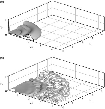
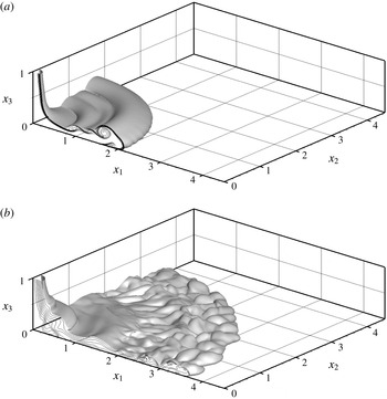
Figure 1 shows a side view of the initial configuration of the cylindrical gravity currents. After the removal of the lock, a cylindrical gravity current, which propagates radially outward across the bottom boundary, is produced. Figure 2 shows one-quarter of the cylindrical gravity current at
 ${\mathcal{C}}=0$
and
 $Re=4000$
visualized by a density isosurface of
 $\unicode[STIX]{x1D70C}=0.15$
. Alternatively, the propagation of gravity currents can be observed using quantities averaged in the wall-normal and in the azimuthal directions. For any flow variable
 $f$
, its average in the wall-normal direction is
 $$\begin{eqnarray}\displaystyle \hat{f}(x_{1},x_{2})=\int _{0}^{1}f(x_{1},x_{2},x_{3})\,\text{d}x_{3}, & & \displaystyle\end{eqnarray}$$
and its average in the azimuthal direction is
 $$\begin{eqnarray}\displaystyle \bar{f}(r,x_{3})=\frac{1}{2\unicode[STIX]{x03C0}}\int _{0}^{2\unicode[STIX]{x03C0}}f(r,\unicode[STIX]{x1D703},x_{3})\,\text{d}\unicode[STIX]{x1D703}, & & \displaystyle\end{eqnarray}$$
where
 $(r,\unicode[STIX]{x1D703},x_{3})$
is converted from
 $(x_{1},x_{2},x_{3})$
in a consistent way as the velocity in cylindrical coordinates
 $(u_{r},u_{\unicode[STIX]{x1D703}},u_{3})$
is converted from
 $(u_{1},u_{2},u_{3})$
.
Cylindrical gravity current at
 ${\mathcal{C}}=0$
and
 $Re=4000$
visualized in one quadrant of the computational domain by the isosurface of
 $\unicode[STIX]{x1D70C}=0.15$
. For illustrative purposes, time instances are chosen at
 $t=3.14$
,
 $9.42$
(a,b). Density contours are also shown by solid lines in the
 $(x_{1},x_{3})$
plane.

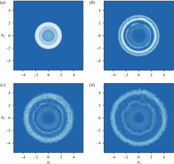
Cylindrical gravity current at
 ${\mathcal{C}}=0$
and
 $Re=4000$
visualized by the density averaged in the wall-normal direction, i.e.
 $\hat{\unicode[STIX]{x1D70C}}(x_{1},x_{2})$
, plotted on the (
 $x_{1}$
,
 $x_{2}$
) plane. For illustrative purposes, time instances are chosen at
 $t=3.14$
,
 $6.44$
,
 $9.42$
,
 $11.66$
(a–d).

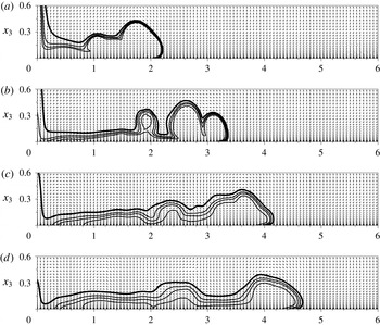
Cylindrical gravity current at
 ${\mathcal{C}}=0$
and
 $Re=4000$
visualized by the density and velocity averaged in the azimuthal direction, i.e.
 $\bar{\unicode[STIX]{x1D70C}}(r,x_{3})$
,
 $\bar{u}_{r}(r,x_{3})$
and
 $\bar{u}_{3}(r,x_{3})$
, plotted on the
 $(r,x_{3})$
plane. For illustrative purposes, time instances are chosen at
 $t=3.14$
,
 $6.44$
,
 $9.42$
,
 $11.66$
(a–d). Density contours are shown by the solid lines and velocity is shown by the vector field on the
 $(r,x_{3})$
plane.

Figure 3 shows the density averaged in the wall-normal direction and figure 4 shows the density and velocity averaged in the azimuthal direction at different time instances for a non-rotating cylindrical gravity current at
 $Re=4000$
. Initially after the heavy fluid is released, the non-rotating cylindrical gravity current evolves as a nearly axisymmetric flow in which Kelvin–Helmholtz vortices develop along the front and body of the current. On propagating further outwards, the cylindrical gravity current acquires a characteristic shape which consists of a raised, bulbous front followed by a much thinner body of the current. It is known from Cantero et al. (Reference Cantero, Balachandar and Garcia2007a
) that, for sufficiently high Reynolds numbers, the non-rotating cylindrical gravity currents are only ‘statistically’ axisymmetric, especially after the slumping phase, in that variations in the azimuthal direction are observed, e.g. the lobe-and-cleft structure; otherwise, for sufficiently low Reynolds numbers, the produced cylindrical gravity currents exhibit perfect axisymmetry. For non-rotating cylindrical gravity currents, we performed simulations only for the case of
 $Re=4000$
for validation and comparison purposes. It has been observed by Cantero et al. (Reference Cantero, Balachandar and Garcia2007a
) that, for non-rotating cylindrical gravity currents, the number of Kelvin–Helmholtz vortices increases with increasing Reynolds numbers.
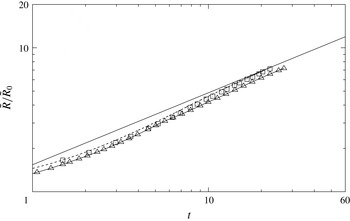
Radius of the advancing front of the cylindrical gravity current at
 ${\mathcal{C}}=0$
as a function of time. The radius is normalized by
 $\tilde{R}_{0}$
and time is normalized by
 $\tilde{H}\tilde{u} _{b}^{-1}$
. Reynolds number is chosen at
 $Re=4000$
in the simulation and at
 $Re\approx O(10^{5})$
in the experiments. Simulation results (▵) are compared with the experimental data (▫) of Hallworth et al. (Reference Hallworth, Huppert and Ungarish2001), with the shallow-water predictions of Ungarish (Reference Ungarish2007), represented by the dashed line and with the theoretical relationship (1.1), represented by the straight solid line.

Figure 5 shows a log–log plot of the front location as a function of time for simulation results, shallow-water predictions and experimental data from Hallworth et al. (Reference Hallworth, Huppert and Ungarish2001). It should be noted that the Reynolds number in the experiments of Hallworth et al. (Reference Hallworth, Huppert and Ungarish2001) is
 $Re\approx O(10^{5})$
, which is significantly larger than
 $Re=4000$
in the corresponding simulations for the non-rotating cylindrical gravity currents. Nevertheless, the simulation results show good agreement with the experimental data and with the theoretical relationship (1.1). It is worth noting that the shallow-water predictions for the non-rotating cylindrical gravity current seem to be in better agreement with the experiment than the solid line.
Cylindrical gravity current at
 ${\mathcal{C}}=0.2$
and
 $Re=4000$
visualized in one quadrant of the computational domain by the isosurface of
 $\unicode[STIX]{x1D70C}=0.15$
. For illustrative purposes, time instances are chosen at
 $t=3.14$
,
 $9.42$
(a,b), which correspond to
 $\unicode[STIX]{x1D6FA}t/2\unicode[STIX]{x03C0}\approx 0.10$
,
 $0.30$
, respectively. Density contours are also shown by solid lines in the
 $(x_{1},x_{3})$
plane.

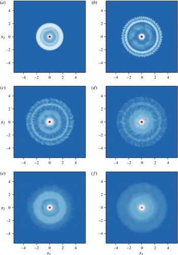
Cylindrical gravity current at
 ${\mathcal{C}}=0.2$
and
 $Re=4000$
visualized by the density averaged in the wall-normal direction, i.e.
 $\hat{\unicode[STIX]{x1D70C}}(x_{1},x_{2})$
, plotted on the (
 $x_{1}$
,
 $x_{2}$
) plane. Time instances are chosen at
 $t=3.14$
,
 $6.44$
,
 $9.42$
,
 $11.66$
,
 $16.34$
,
 $24.82$
(a–f), which correspond to
 $\unicode[STIX]{x1D6FA}t/2\unicode[STIX]{x03C0}\approx 0.10$
,
 $0.20$
,
 $0.30$
,
 $0.37$
,
 $0.52$
,
 $0.79$
, respectively.

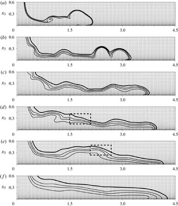
Cylindrical gravity current at
 ${\mathcal{C}}=0.2$
and
 $Re=4000$
visualized by the density and velocity averaged in the azimuthal direction, i.e.
 $\bar{\unicode[STIX]{x1D70C}}(r,x_{3})$
,
 $\bar{u}_{r}(r,x_{3})$
and
 $\bar{u}_{3}(r,x_{3})$
, plotted on the
 $(r,x_{3})$
plane. For illustrative purposes, time instances are chosen at
 $t=3.14$
,
 $6.44$
,
 $9.42$
,
 $11.66$
,
 $16.34$
,
 $24.82$
(a–f), which correspond to
 $\unicode[STIX]{x1D6FA}t/2\unicode[STIX]{x03C0}\approx 0.10$
,
 $0.20$
,
 $0.30$
,
 $0.37$
,
 $0.52$
,
 $0.79$
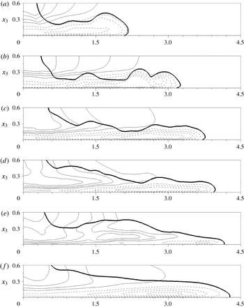
, respectively. Density contours are shown by the solid lines, where the thick solid line represents
 $\bar{\unicode[STIX]{x1D70C}}=0.01$
, and velocity is shown by the vector field on the
 $(r,x_{3})$
plane. The dashed boxes at
 $t=11.66$
and
 $16.34$
indicate the leading edge of the new pulse.

Cylindrical gravity current at
 ${\mathcal{C}}=0.2$
and
 $Re=4000$
visualized by the density and tangential velocity averaged in the azimuthal direction, i.e.
 $\bar{\unicode[STIX]{x1D70C}}(r,x_{3})$
and
 $\bar{u}_{\unicode[STIX]{x1D703}}(r,x_{3})$
, plotted on the
 $(r,x_{3})$
plane. For illustrative purposes, time instances are chosen at
 $t=3.14$
,
 $6.44$
,
 $9.42$
,
 $11.66$
,
 $16.34$
,
 $24.82$
(a–f), which correspond to
 $\unicode[STIX]{x1D6FA}t/2\unicode[STIX]{x03C0}\approx 0.10$
,
 $0.20$
,
 $0.30$
,
 $0.37$
,
 $0.52$
,
 $0.79$
, respectively. The thick solid line represents the density contour of
 $\bar{\unicode[STIX]{x1D70C}}=0.01$
and the thin solid (dashed) lines represent counterclockwise (clockwise or retrograde) tangential velocity across the
 $(r,x_{3})$
plane, in the rotating frame of reference.

3.2 Rotating cylindrical gravity currents
For rotating cylindrical gravity currents produced by a full-depth lock release, we focus attention on the situation when the ratio of Coriolis to inertia forces is not large. Three different ratios of Coriolis to inertia forces are considered in this study, namely
 ${\mathcal{C}}=0.1,0.2,0.3$
. These rotating cylindrical gravity currents exhibit special features, including a maximum radius of propagation and a regular series of outwardly propagating pulses, that are qualitatively distinct from the non-rotating cylindrical gravity currents. Since the flow patterns among the rotating cases are qualitatively similar, we present the detailed flow information only for the case of
 ${\mathcal{C}}=0.2$
and other details for
 ${\mathcal{C}}=0.1,0.3$
are omitted for brevity.
Figure 6 shows one-quarter of the cylindrical gravity current at
 ${\mathcal{C}}=0.2$
and
 $Re=4000$
visualized by a density isosurface of
 $\unicode[STIX]{x1D70C}=0.15$
. Before the lock is removed, the system is in solid-body rotation and both heavy and light fluids are quiescent in the rotating frame of reference. Initially after the heavy fluid is released, the rotating cylindrical gravity current collapses in a similar way as the non-rotating cylindrical gravity current in that the flow spreads radially outward axisymmetrically with Kelvin–Helmholtz vortices developing along the front and body of the current. However, as the rotating cylindrical gravity current propagates further outward, striking differences from the non-rotating case emerge. The rotating cylindrical gravity current maintains a core region of heavy fluid at the centre of rotation and the body of the current is no longer thin compared with the front. It is worth noting here that for a full-depth lock release in a rotating system, the observed core region of heavy fluid at the centre of rotation confirms the observation of a ‘point of surface contact’ for rotating cylindrical gravity currents produced from a full-depth lock release in the laboratory (Saunders Reference Saunders1973; Dewar & Killworth Reference Dewar and Killworth1990) but we should keep in mind that only a small portion of heavy fluid is contained in this region (Ungarish Reference Ungarish2009). Conservation of angular momentum requires acceleration in the tangential velocity of a fluid of which the radius decreases and deceleration of a fluid of which the radius increases. Therefore, in the rotating frame of reference, with the system rotating in the clockwise direction, the contracting fluid acquires a counterclockwise rotation while the expanding fluid acquires a clockwise rotation. For a partial-depth lock release, as demonstrated by Hallworth et al. (Reference Hallworth, Huppert and Ungarish2001), such a core region of heavy fluid at the centre does not appear. From the comparison between figures 2 and 6, it is observed that the Coriolis effects modify the profile of the cylindrical gravity current from one which has the front as the most prominent feature of the current with a much thinner body to another of which the thickness of the current decreases in the radially outward direction. The difference in the front location between figures 2 and 6 may not be very easily visualized but the radius of the front versus time, as plotted in figure 10, shows a sensible difference between the non-rotating and rotating cases when
 $\unicode[STIX]{x1D6FA}t/2\unicode[STIX]{x03C0}\gtrsim 0.2$
.
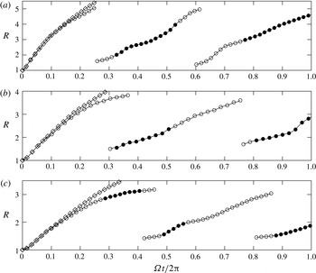
The radius of the advancing front and the leading edge of subsequent pulses of rotating cylindrical gravity currents,
 $R$
, plotted against time in terms of the fraction of one revolution that the system has rotated through, i.e.
 $\unicode[STIX]{x1D6FA}t/2\unicode[STIX]{x03C0}$
. The radius of the advancing front and the leading edge of subsequent pulses are non-dimensionalized by the lock height
 $\tilde{H}$
. The angular velocity of the rotating system and time are non-dimensionalized by the time scale
 $\tilde{H}\tilde{u} _{b}^{-1}$
. The Reynolds number in the simulations is chosen at
 $Re=4000$
. Results for three different ratios of Coriolis to inertia forces are presented in (a),
 ${\mathcal{C}}=0.1$
; (b),
 ${\mathcal{C}}=0.2$
; (c),
 ${\mathcal{C}}=0.3$
. Symbols: ○, the radius of the advancing front and the leading edge of subsequent pulses of rotating cylindrical gravity currents; ●, the radius of the front and subsequent pulses while the potential energy in the system is increasing; ♢, the radius of the advancing front of the non-rotating cylindrical gravity current at
 $Re=4000$
.

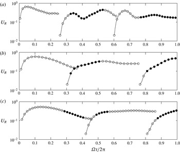
The velocity of the advancing front and the leading edge of subsequent pulses of rotating cylindrical gravity currents,
 $U_{R}$
, plotted against time in terms of the fraction of one revolution that the system has rotated through, i.e.
 $\unicode[STIX]{x1D6FA}t/2\unicode[STIX]{x03C0}$
. The velocity of the advancing front and the leading edge of subsequent pulses are non-dimensionalized by
 $\tilde{u} _{b}$
. The angular velocity of the rotating system and time are non-dimensionalized by the time scale
 $\tilde{H}\tilde{u} _{b}^{-1}$
. The Reynolds number in the simulations is chosen at
 $Re=4000$
. Results for three different ratios of Coriolis to inertia forces are presented in (a),
 ${\mathcal{C}}=0.1$
; (b),
 ${\mathcal{C}}=0.2$
; (c),
 ${\mathcal{C}}=0.3$
. Symbols: ○, the velocity of the advancing front and the leading edge of subsequent pulses of rotating cylindrical gravity currents; ●, the velocity of the front and subsequent pulses while the potential energy in the system is increasing.

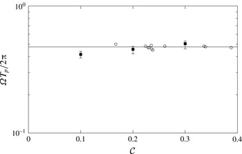
The pulse period, in terms of
 $\unicode[STIX]{x1D6FA}T_{p}/2\unicode[STIX]{x03C0}$
, plotted against the ratio of Coriolis to inertia forces,
 ${\mathcal{C}}$
, for rotating cylindrical gravity currents. The angular velocity of the rotating system and time are non-dimensionalized by the time scale
 $\tilde{H}\tilde{u} _{b}^{-1}$
. The variable
 $\unicode[STIX]{x1D6FA}T_{p}/2\unicode[STIX]{x03C0}$
represents the pulse period in terms of the fraction of one revolution that the system has rotated through. Symbols: ○, results from experiments reported by Hallworth et al. (Reference Hallworth, Huppert and Ungarish2001); ▪, present simulation results. The Reynolds number in the simulations for the rotating cylindrical gravity currents is chosen at
 $Re=4000$
and the Reynolds number in the experiments is at
 $Re\approx O(10^{5})$
. Solid line represents
 $\unicode[STIX]{x1D6FA}T_{p}/2\unicode[STIX]{x03C0}\approx 0.476$
given by Hallworth et al. (Reference Hallworth, Huppert and Ungarish2001).

In order to better understand the dynamical processes in the propagation, figure 7 shows the density averaged in the wall-normal direction and figures 8 and 9 show the density and velocity averaged in the azimuthal direction at different time instances for a cylindrical gravity current at
 ${\mathcal{C}}=0.2$
and
 $Re=4000$
. Prior to
 $t\approx 3.14$
or
 $\unicode[STIX]{x1D6FA}t/2\unicode[STIX]{x03C0}\approx 0.10$
, both non-rotating and rotating cylindrical gravity currents exhibit nearly perfect axisymmetry in flow patterns and the Kelvin–Helmholtz vortices along the front and body of the current do not undergo bending and tilting processes at this stage of flow. As the rotating cylindrical gravity current propagates further outward, at
 $t\approx 6.44$
or
 $\unicode[STIX]{x1D6FA}t/2\unicode[STIX]{x03C0}\approx 0.20$
, the outer rim of the spreading heavy fluid breaks away from the body of the current. The detached outer rim of heavy fluid continues to move outward but decelerates rapidly until a maximum radius of propagation is attained, at
 $t\approx 11.66$
or
 $\unicode[STIX]{x1D6FA}t/2\unicode[STIX]{x03C0}\approx 0.37$
. The determination of the maximum radius of propagation requires a subjective judgement by viewing the movies of density and velocity fields, since the decelerating heavy fluid stagnates and gently diffuses around the maximum radius of propagation. Our observation agrees faithfully with the laboratory experiments by Hallworth et al. (Reference Hallworth, Huppert and Ungarish2001), who reported that a residue of heavy fluid sticks around the maximum radius of propagation of which the position becomes ambiguous. The time at which rotating cylindrical gravity currents attain a maximum radius of propagation,
 $T_{max}$
, is found to depend on the ratio of Coriolis to inertia forces. As will be shown in figure 10, a maximum radius is attained at
 $\unicode[STIX]{x1D6FA}T_{max}/2\unicode[STIX]{x03C0}\approx 0.25$
for the case of
 ${\mathcal{C}}=0.1$
and
 $Re=4000$
and at
 $\unicode[STIX]{x1D6FA}T_{max}/2\unicode[STIX]{x03C0}\approx 0.45$
for the case of
 ${\mathcal{C}}=0.3$
and
 $Re=4000$
. It is shown in figure 9 that, before
 $t\approx 11.66$
or
 $\unicode[STIX]{x1D6FA}t/2\unicode[STIX]{x03C0}\approx 0.37$
, the Coriolis effects result in a retrograde azimuthal motion of the spreading heavy fluid, relative to the rotating system, while the direction of tangential velocity in the core region is concurrent with the rotating system.
The body of the current begins to contract radially inward toward the centre of rotation as the advancing front approaches the maximum radius of propagation. The contraction of the body of the current is a complex rearrangement process of the heavy fluid. As figures 8 and 9 show at
 $t\approx 11.66$
or
 $\unicode[STIX]{x1D6FA}t/2\unicode[STIX]{x03C0}\approx 0.37$
, while the body of the current contracts radially inward, the heavy fluid in the upper part of the body of the current near the centre of rotation forms a new pulse at
 $r\approx 1.7$
and begins to move radially outward. The determination of the location of the new pulse requires a careful interpretation of the density field in conjunction with the velocity field. Here the new pulse location is determined to be the furthest radial location at which the new pulse maintains a positive radially outward buoyancy flux. As shown by the dashed box in figure 8 at
 $t=11.66$
in the range of
 $1.5\lesssim r\lesssim 2.1$
, the heavy fluid of the new pulse in the region of
 $r\lesssim 1.7$
maintains a positive outward flux while in the region of
 $r\gtrsim 1.7$
, the heavy fluid is contracting and the buoyancy flux is radially inward. Therefore, the location of the new pulse at
 $t\approx 11.66$
in figure 8 is determined to be at
 $r\approx 1.7$
.
The new pulse near the centre of rotation in the upper part of the body of the current continues to push outward against the inward contracting heavy fluid, while the thickness of the current increases in the region where the outward propagating new pulse and the inward contracting flow converge. At
 $t\approx 16.34$
or
 $\unicode[STIX]{x1D6FA}t/2\unicode[STIX]{x03C0}\approx 0.52$
, the new pulse has reached
 $r\approx 2.4$
, as shown in figures 8 and 9. Here the location of the new pulse is determined again in the way described above. Afterwards, while the outer part of the heavy fluid continues propagating radially outward, the inner part of the heavy fluid close to the centre of rotation contracts radially inward and another new pulse begins to form at
 $r\approx 1.8$
, as shown in figure 8 at
 $t=24.82$
or
 $\unicode[STIX]{x1D6FA}t/2\unicode[STIX]{x03C0}\approx 0.79$
. It is worth noting that the new pulse of heavy fluid does not break away from the body of the current, which occurs only once before the initial advancing front approaches the maximum radius of propagation. The contraction–relaxation motion and the outward propagating new pulses are repeated regularly several times, as confirmed by experimental observations reported in Hallworth et al. (Reference Hallworth, Huppert and Ungarish2001).
The radius and the velocity of the advancing front and the leading edge of subsequent pulses against time in terms of the fraction of one revolution that the system has rotated through, i.e.
 $\unicode[STIX]{x1D6FA}t/2\unicode[STIX]{x03C0}$
, for cylindrical gravity currents at
 ${\mathcal{C}}=0.1,0.2,0.3$
and
 $Re=4000$
are plotted in figures 10 and 11, respectively. The velocity of the front and subsequent pulses are derived from the radius of the front and pulses via
 $U_{R}=\text{d}R/\text{d}t$
. The radius of the advancing front of the non-rotating cylindrical gravity current at
 $Re=4000$
is also included in figure 10 for comparison. During the initial one-tenth of a revolution of the system, the Coriolis effects are not significant in terms of the front location history. For rotating cylindrical gravity currents, the averaged time interval between the arrival of successive fronts, i.e. the pulse period
 $T_{p}$
, can be determined. Figure 12 shows the pulse period, in terms of
 $\unicode[STIX]{x1D6FA}T_{p}/2\unicode[STIX]{x03C0}$
, against the ratio of Coriolis to inertia forces in the rotating system. Interestingly, it is observed that the subsequent pulses form and propagate radially outward in a period slightly less than a half-revolution of the system. Such an observation is in accordance with Hallworth et al. (Reference Hallworth, Huppert and Ungarish2001), who reported that
 $\unicode[STIX]{x1D6FA}T_{p}/2\unicode[STIX]{x03C0}\approx 0.476$
, and explains that these subsequent pulses are related to the inertial oscillations in a rotating system, of which the inertial frequency is
 $2\unicode[STIX]{x1D6FA}$
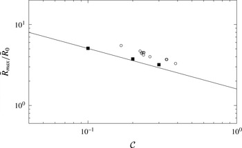
. Figure 13 shows the maximum radius of propagation against the ratio of Coriolis to inertia forces. The theoretical relationship (1.4) appropriately describes the simulation and experimental results.
Maximum radius of propagation,
 $\tilde{R}_{max}/\tilde{R}_{0}$
, plotted against the ratio of Coriolis to inertia forces,
 ${\mathcal{C}}$
, for rotating cylindrical gravity currents. Symbols: ○, results from experiments reported by Hallworth et al. (Reference Hallworth, Huppert and Ungarish2001); ▪, present simulation results. The Reynolds number in the simulations for the rotating cylindrical gravity currents is chosen at
 $Re=4000$
and the Reynolds number in the experiments is at
 $Re\approx O(10^{5})$
. Solid line represents the theoretical prediction (1.4) given by Ungarish & Huppert (Reference Ungarish and Huppert1999).

3.3 Energy budgets
From the point of view of energy budgets, the propagation of cylindrical gravity currents in a rotating system is a conversion process of the potential energy into kinetic energy and subsequently into dissipation by viscous friction, essentially in a similar way as non-rotating cylindrical gravity currents but subject to the Coriolis effects. Information on the energy budgets can be difficult to attain in the experiments on a rotating turntable. In the literature, such an attempt has been made successfully in the laboratory by Stegner et al. (Reference Stegner, Bouruet-Aubertot and Pichon2004), who quantify the final energy budget after an adjustment process with the help of visualization techniques. Energy budgets based on the shallow-water formulation are also discussed in Ungarish (Reference Ungarish2009). However, a complete and time-dependent energy budget is still sought and is now possible thanks to the three-dimensional high-resolution simulations. In the following we will provide a computational analysis of the energy budget for rotating cylindrical gravity currents.
The equation for the time derivative of the kinetic energy is obtained by multiplying the momentum (2.2) by
 $u_{i}$
, i.e.
 $$\begin{eqnarray}\displaystyle \frac{\text{D}}{\text{D}t}\left(\frac{1}{2}u_{i}u_{i}\right)=-\frac{\unicode[STIX]{x2202}}{\unicode[STIX]{x2202}x_{i}}(pu_{i})+\frac{2}{Re}\frac{\unicode[STIX]{x2202}}{\unicode[STIX]{x2202}x_{j}}(\unicode[STIX]{x1D634}_{ij}u_{i})-\frac{2}{Re}\unicode[STIX]{x1D634}_{ij}\unicode[STIX]{x1D634}_{ij}-\unicode[STIX]{x1D70C}u_{3}, & & \displaystyle\end{eqnarray}$$
where
 $\text{D}/\text{D}t$
denotes the material derivative,
 $\unicode[STIX]{x1D634}_{ij}$
denotes the strain rate tensor,
 $\unicode[STIX]{x1D634}_{ij}=(u_{i,j}+u_{j,i})/2$
and
 $u_{3}$
denotes the velocity component in
 $x_{3}$
direction. It is interesting to note that the Coriolis term in (2.2) vanishes when multiplied by
 $u_{i}$
and therefore the energy (3.3) has the same form as that for gravity currents in a non-rotating system. Integration of (3.3) over the entire flow domain
 ${\mathcal{V}}$
leads to the evolution equation of the total kinetic energy
 $E_{k}$
, i.e.
 $$\begin{eqnarray}\displaystyle \frac{\text{d}E_{k}}{\text{d}t}=-\frac{2}{Re}\int _{{\mathcal{V}}}\unicode[STIX]{x1D634}_{ij}\unicode[STIX]{x1D634}_{ij}\,\text{d}V-\int _{{\mathcal{V}}}\unicode[STIX]{x1D70C}u_{3}\,\text{d}V,\quad E_{k}(t)=\int _{{\mathcal{V}}}\frac{1}{2}u_{i}u_{i}\,\text{d}V, & & \displaystyle\end{eqnarray}$$
where the divergence terms on the right-hand side of (3.3) vanish after integration. By weighting the kinetic energy with the dimensionless density, we can associate a fraction of the kinetic energy with the heavy fluid, i.e.
 $$\begin{eqnarray}\displaystyle E_{k_{H}}=\int _{{\mathcal{V}}}\frac{1}{2}\unicode[STIX]{x1D70C}u_{i}u_{i}\,\text{d}V, & & \displaystyle\end{eqnarray}$$
and the remainder of the total kinetic energy is associated with the ambient fluid. When the effects of diffusion in the density field on the potential energy is neglected (Winters et al. Reference Winters, Lombard, Riley and D’Asaro1995; Birman, Martin & Meiburg Reference Birman, Martin and Meiburg2005; Dai Reference Dai2015; Dai & Huang Reference Dai and Huang2016), the time derivative of the potential energy in the system is
 $$\begin{eqnarray}\displaystyle \frac{\text{d}E_{p}}{\text{d}t}=\int _{{\mathcal{V}}}\unicode[STIX]{x1D70C}u_{3}\,\text{d}V,\quad E_{p}(t)=\int _{{\mathcal{V}}}\unicode[STIX]{x1D70C}x_{3}\,\text{d}V. & & \displaystyle\end{eqnarray}$$
The first term on the right-hand side of (3.4) represents the dissipation rate and we use
 $E_{d}$
to denote the time integral of dissipation rate, i.e.
 $$\begin{eqnarray}\displaystyle E_{d}(t)=\int _{0}^{t}\unicode[STIX]{x1D716}(\unicode[STIX]{x1D70F})\,\text{d}\unicode[STIX]{x1D70F},\quad \unicode[STIX]{x1D716}=\frac{2}{Re}\int _{{\mathcal{V}}}\unicode[STIX]{x1D634}_{ij}\unicode[STIX]{x1D634}_{ij}\,\text{d}V. & & \displaystyle\end{eqnarray}$$
In other words, equation (3.4) is essentially a statement of conservation of energy, i.e. that
 $E_{k}+E_{p}+E_{d}$
is a constant in the adjustment processes of rotating cylindrical gravity currents.
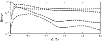
The normalized potential energy
 $E_{p}^{n}$
(▫), kinetic energy
 $E_{k}^{n}$
(▿), kinetic energy associated with heavy fluid
 $E_{kH}^{n}$
(▵) and dissipation rate
 $\unicode[STIX]{x1D716}^{n}=\text{d}E_{d}^{n}/\text{d}t$
(○) plotted against time in terms of the fraction of one revolution that the system has rotated through, i.e.
 $\unicode[STIX]{x1D6FA}t/2\unicode[STIX]{x03C0}$
, for rotating cylindrical gravity currents at
 ${\mathcal{C}}=0.2$
and
 $Re=4000$
.

Since the energy budgets for rotating cylindrical gravity currents are qualitatively similar for all ratios of Coriolis to inertia forces considered in this study, here we focus on the case of rotating cylindrical gravity currents at
 ${\mathcal{C}}=0.2$
and
 $Re=4000$
and other cases are not discussed here in detail for brevity. Figure 14 shows the time histories of the normalized potential energy, kinetic energy, kinetic energy associated with heavy fluid and dissipation rate during the propagation of rotating cylindrical gravity currents at
 ${\mathcal{C}}=0.2$
and
 $Re=4000$
. The energy budgets are normalized with the initial potential energy in the system and the superscript n denotes normalized contributions. The overall energy in the simulations is observed to be conserved to a high degree of accuracy. The maximum error in the overall energy is within
 $5\,\%$
and can be attributed mainly to the fact that the effects of diffusion in the density field on the potential energy are neglected. As the heavy fluid initially collapses radially outward, the kinetic energy increases at the expense of decreasing potential energy. As the outer rim of the spreading heavy fluid breaks away from the body of the current, at
 $t\approx 6.44$
or
 $\unicode[STIX]{x1D6FA}t/2\unicode[STIX]{x03C0}\approx 0.21$
, the dissipation rate reaches its maximum value. As the detached outer rim of heavy fluid approaches a maximum radius of propagation, the potential energy in the rotating system reaches a local minimum, at
 $t\approx 9.42$
or
 $\unicode[STIX]{x1D6FA}t/2\unicode[STIX]{x03C0}\approx 0.30$
and a new pulse of heavy fluid begins to form near the centre of rotation at
 $r\approx 1.5$
, cf. figures 8 and 9 at
 $t=9.42$
. The new pulse of heavy fluid initially moves radially outward over the contracting body of the current and the potential energy in the system increases at the expense of decreasing kinetic energy until a local maximum of potential energy is reached, at
 $t\approx 16.34$
or
 $\unicode[STIX]{x1D6FA}t/2\unicode[STIX]{x03C0}\approx 0.52$
, approximately when the kinetic energy reaches a local minimum value. The radius of the advancing front and the leading edge of subsequent pulses, while the potential energy in the system is increasing, is highlighted with closed symbols in figure 10. It is worth noting that, the contraction–relaxation motion may be initiated after the attainment of a maximum radius of propagation for
 ${\mathcal{C}}=0.1,0.2$
, while the contraction–relaxation motion may also be initiated before the attainment of a maximum radius of propagation for
 ${\mathcal{C}}=0.3$
. During the latter part of the new pulse propagation, the heavy fluid accumulated in the new pulse relaxes and the kinetic energy in the system increases at the expense of decreasing potential energy until a local minimum of potential energy is reached, at
 $t\approx 24.82$
or
 $\unicode[STIX]{x1D6FA}t/2\unicode[STIX]{x03C0}\approx 0.79$
, approximately when the kinetic energy reaches a local maximum value and another new pulse of heavy fluid takes form.
For the rotating cylindrical gravity currents, due to the Coriolis effects, the potential energy in the system does not decrease monotonically but shows a cyclic pattern of rise and fall consistent with the contraction–relaxation process of the heavy fluid. Based on the simulation results, it is observed that during the contraction–relaxation motion of the heavy fluid, the normalized potential energy oscillates in the range of
 $0.14\lesssim E_{p}^{n}\lesssim 0.15$
for
 ${\mathcal{C}}=0.1$
,
 $0.21\lesssim E_{p}^{n}\lesssim 0.24$
for
 ${\mathcal{C}}=0.2$
and
 $0.29\lesssim E_{p}^{n}\lesssim 0.33$
for
 ${\mathcal{C}}=0.3$
for the rotating cylindrical gravity currents at
 $Re=4000$
considered in this study. The fraction of initial potential energy, that is retained in the rotating system after the heavy fluid is released, increases as the ratio of Coriolis to inertia forces increases. It should be noted that, although the kinetic energy shows local maximum and minimum values as does the potential energy, the sum of kinetic energy and potential energy, i.e.
 $E_{k}+E_{p}$
, is decreasing over time due to the dissipation. While the potential energy in the system oscillates in a fixed range, it is mainly the kinetic energy that is consumed by the dissipation, as shown by the decreasing kinetic energy in figure 14. As also confirmed by laboratory experiments, these new pulses are generated repeatedly in the rotating cylindrical gravity currents and the above transformation between potential energy and kinetic energy, where the kinetic energy in the system is decreasing due to the dissipation, is likewise repeated as the contraction–relaxation process continues.
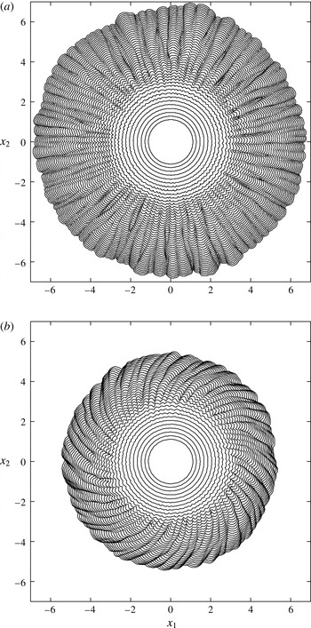
Composite picture on the
 $(x_{1},x_{2})$
plane of the leading edge of the non-rotating and rotating cylindrical gravity currents over time. The non-rotating case (
 ${\mathcal{C}}=0$
) is shown in panel (a) and the rotating case (
 ${\mathcal{C}}=0.1$
) is shown in panel (b). Front location is visualized by contours of
 $\unicode[STIX]{x1D70C}=0.01$
close to the bottom at
 $x_{3}=0.012$
. Time separation between consecutive contours is chosen at
 $\unicode[STIX]{x0394}t=0.495$
. For illustrative purposes, the last outer contour in panel (a) is chosen at
 $t=20.79$
and the last outer contour in panel (b) is chosen at
 $t=18.74$
. The Reynolds number in the simulations of the non-rotating and rotating cylindrical gravity currents is chosen at
 $Re=4000$
.

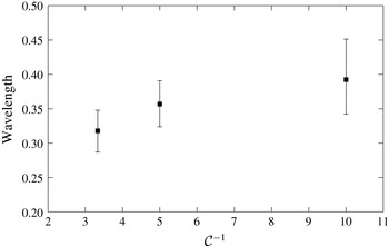
The wavelength of the lobes for
 $Re=4000$
plotted against the inverse of the ratio of Coriolis to inertia forces. Note that the deformation radius,
 $\tilde{R}_{d}$
, is related to the ratio of Coriolis to inertia forces via
 $\tilde{R}_{d}=\tilde{R}_{0}/(2{\mathcal{C}})$
.

3.4 Lobes and clefts and flow structures
The lobe-and-cleft structure is a ubiquitous, three-dimensional feature at the front of gravity currents at sufficiently high Reynolds numbers. The three-dimensional lobe-and-cleft structure of the advancing front can be seen in figures 2 and 6 for the cylindrical gravity currents in non-rotating and rotating systems. To date, it is known that the lobe-and-cleft structure originates in the unstable stratification of a thin layer of light ambient fluid overrun by the leading edge of gravity currents (Simpson Reference Simpson1972; Härtel, Carlsson & Thunblom Reference Härtel, Carlsson and Thunblom2000a
). The leading edge of the cylindrical gravity currents in non-rotating (
 ${\mathcal{C}}=0$
) and rotating (
 ${\mathcal{C}}=0.1$
) systems, identified by the contour of
 $\unicode[STIX]{x1D70C}=0.01$
close to the bottom boundary, is plotted at consecutive times on the
 $(x_{1},x_{2})$
plane in figure 15. The composite picture provides a clear view of the formation of lobes and clefts and captures the splitting and merging of existing lobes and clefts. The major feature of the rotating cylindrical gravity currents, as clearly observed again in figure 15, is the attainment of a maximum radius of propagation. Furthermore, due to the retrograde azimuthal motion of the heavy fluid, relative to the rotating system, the clefts leave a footprint which goes in the clockwise direction on the
 $(x_{1},x_{2})$
plane. It is also observed in figure 15 that merger between existing lobes occurs as the maximum radius of propagation is approached. Laboratory experiments by Stegner et al. (Reference Stegner, Bouruet-Aubertot and Pichon2004) show that the final wavelength of the lobes that occurs just before the contraction stage depends on the deformation radius,
 $\tilde{R}_{d}=\tilde{R}_{0}/(2{\mathcal{C}})$
. From our three-dimensional high-resolution simulations, it is also confirmed that the final wavelength of the lobes for
 $Re=4000$
is proportional to the deformation radius,
 $\tilde{R}_{d}$
, or equivalently, inversely proportional to the ratio of Coriolis to inertia forces,
 ${\mathcal{C}}$
, as shown in figure 16.
Quantitative information on the lobe-and-cleft structure. Time is expressed in terms of the fraction of one revolution that the system has rotated through, i.e.
 $\unicode[STIX]{x1D6FA}t/2\unicode[STIX]{x03C0}$
.
 $R$
is the mean radius of the advancing front and
 $N_{90}$
is the mean number of lobes within a
 $90^{\circ }$
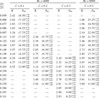
sector, which is averaged over four quadrants of the computational domain. The error estimates are to add and subtract the maximum and minimum values and are not the root-mean-square estimates.

Near-bed flow at the advancing front of the cylindrical gravity currents at
 ${\mathcal{C}}=0$
and
 $Re=4000$
, shown in panel (a), and at
 ${\mathcal{C}}=0.1$
and
 $Re=4000$
, shown in panel (b). The advancing front, represented by the thick solid line, is visualized by the density contour of
 $\unicode[STIX]{x1D70C}=0.015$
close to the bottom at
 $x_{3}=0.012$
. The vector field shows the velocity on the
 $(x_{1},x_{2})$
plane at
 $x_{3}=0.012$
. The thin solid (dashed) lines represent the positive (negative) vertical velocity on the
 $(x_{1},x_{2})$
plane at
 $x_{3}=0.012$
.

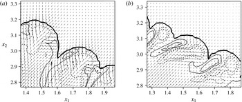
With the help of three-dimensional high-resolution simulations, the flow field in the lobe-and-cleft structure can be visualized. For non-rotating cylindrical gravity currents, it has been observed by Cantero et al. (Reference Cantero, Balachandar and Garcia2007a
) that there exist horizontal flow directed from the centre of each lobe into the two neighbouring clefts, vertically upward flow at the clefts and vertically downward flow at the lobes, as confirmed here in figure 17(a) for the non-rotating cylindrical gravity current at
 $Re=4000$
and at
 $t=7.07$
. For rotating cylindrical gravity currents, the horizontal flow in a lobe near the bed, due to the retrograde azimuthal motion of the heavy fluid, is skewed toward the downwind direction, as shown in figure 17(b) for the rotating cylindrical gravity currents at
 ${\mathcal{C}}=0.1$
and
 $Re=4000$
and also at
 $t=7.07$
. For each cleft in a rotating cylindrical gravity current, there exist vertically upward flow on one side of the cleft and vertically downward flow on the other side of the cleft.
Quantitative information on the number of lobes at selected time instances is presented in table 1. The counting of the number of lobes in rotating cylindrical gravity currents requires a careful interpretation, especially at the incipient stage of merger and splitting of the lobes and clefts due to the complex nature of the structure. For non-rotating cylindrical gravity currents, it was reported previously by Cantero et al. (Reference Cantero, Balachandar and Garcia2007a
) that the number of lobes is maintained over time as the non-rotating cylindrical gravity currents propagate radially outward. For rotating cylindrical gravity currents, table 1 shows that, for the rotating cylindrical gravity currents at
 ${\mathcal{C}}=0.1,0.2,0.3$
and
 $Re=4000$
,
 $8000$
considered in this study, the number of lobes is maintained only for a limited period of time before merger between existing lobes occurs when a maximum radius of propagation is approached.
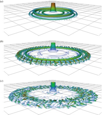
Volumetric rendering of
 $\unicode[STIX]{x1D706}_{ci}$
for the rotating cylindrical gravity current at
 ${\mathcal{C}}=0.2$
and
 $Re=4000$
. For illustrative purposes, time instances are chosen at
 $t=3.14$
,
 $6.44$
,
 $9.42$
(a–c), which correspond to
 $\unicode[STIX]{x1D6FA}t/2\unicode[STIX]{x03C0}\approx 0.10$
,
 $0.20$
,
 $0.30$
, respectively. Spacing between consecutive grid lines in the horizontal directions, i.e.
 $x_{1}$
and
 $x_{2}$
, is chosen at one dimensionless unit.

To better visualize the three-dimensional structure of the rotating cylindrical gravity currents, figure 18 shows the swirling strength for the rotating cylindrical gravity current at
 ${\mathcal{C}}=0.2$
and
 $Re=4000$
. For illustrative purposes, time instances are chosen at
 $t=3.14$
,
 $6.44$
,
 $9.42$
, which correspond to
 $\unicode[STIX]{x1D6FA}t/2\unicode[STIX]{x03C0}\approx 0.10$
,
 $0.20$
,
 $0.30$
, respectively. The swirling strength,
 $\unicode[STIX]{x1D706}_{ci}$
, is the absolute value of the imaginary part of the complex eigenvalues of the velocity gradient tensor and is suitable to pick out regions of intense vorticity (Chakraborty, Balachandar & Adrian Reference Chakraborty, Balachandar and Adrian2005). It is clear from figure 18 that the Kelvin–Helmholtz vortices maintain nearly perfect axisymmetry prior to
 $\unicode[STIX]{x1D6FA}t/2\unicode[STIX]{x03C0}\approx 0.10$
. As the maximum radius of propagation is approached, three-dimensionality of the flow quickly develops. Furthermore, there exist quasi-streamwise vortices winding around the Kelvin–Helmholtz vortices and leading to break up process of the vortex structures, as shown in figure 18 at
 $t=6.44$
or
 $\unicode[STIX]{x1D6FA}t/2\unicode[STIX]{x03C0}\approx 0.20$
. Such quasi-streamwise vortices do not have counterparts in the non-rotating cylindrical gravity currents.
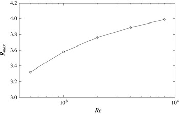
Maximum radius of propagation,
 $R_{max}$
, against the Reynolds number,
 $Re$
, for the rotating cylindrical gravity currents at
 ${\mathcal{C}}=0.2$
.

3.5 Influence of the Reynolds number
The propagation of the rotating cylindrical gravity currents can be expected to vary with the Reynolds number, due to the changing balance between the inertial and viscous forces. Here we examine how the above picture of the rotating cylindrical gravity currents depends on the Reynolds number. To do this, we restrict our attention to the rotating cylindrical gravity currents with the ratio of Coriolis to inertia forces maintained at
 ${\mathcal{C}}=0.2$
and the Reynolds number varied at five different values of
 $500$
,
 $1000$
,
 $2000$
,
 $4000$
and
 $8000$
.
For the lowest two Reynolds numbers of
 $500$
and
 $1000$
considered in this study, the rotating cylindrical gravity current propagates radially outward in a way consistent with the other higher Reynolds numbers of
 $2000$
,
 $4000$
and
 $8000$
. However, the number of vortices forming due to the roll up of the interface appears to increase with increasing Reynolds number. During the initial one-tenth of a revolution of the system, except that no Kelvin–Helmholtz vortex develops at
 $Re=500$
, there are two, three, four and five Kelvin–Helmholtz vortices forming at the interface between the heavy and light fluids for
 $Re=1000$
,
 $2000$
,
 $4000$
and
 $8000$
, respectively. Furthermore, at
 $Re=500$
,
 $1000$
, the rotating cylindrical gravity currents remain perfectly axisymmetric throughout the simulation and the outer rim of spreading heavy fluid does not break away from the body of the current while at the other higher Reynolds numbers three-dimensionality of the flow quickly develops after the initial one-tenth of a revolution of the system.
The number of lobes, as listed in table 1, is found to increase with increasing Reynolds number for rotating cylindrical gravity currents at
 ${\mathcal{C}}=0.2$
and
 $Re=4000$
,
 $8000$
. The maximum radius of propagation,
 $R_{max}$
, for the
 ${\mathcal{C}}=0.2$
case, as shown in figure 19, increases with increasing Reynolds number and the time required to reach the maximum radius of propagation,
 $T_{max}$
, increases from
 $\unicode[STIX]{x1D6FA}T_{max}/2\unicode[STIX]{x03C0}\approx 0.341$
at
 $Re=500$
to
 $\unicode[STIX]{x1D6FA}T_{max}/2\unicode[STIX]{x03C0}\approx 0.378$
at
 $Re=8000$
. Our results indicate that the influence of the Reynolds number diminishes as
 $Re$
increases, which is consistent with previously published reports, e.g. Birman et al. (Reference Birman, Martin and Meiburg2005) and Dai (Reference Dai2015), that the influence of the Reynolds number is weak for
 $Re\gtrsim 4000$
.
4 Conclusions
Cylindrical gravity currents, produced by a full-depth lock release, in a rotating system are investigated by means of three-dimensional high-resolution simulations of the incompressible variable-density Navier–Stokes equations with the Coriolis term and using the Boussinesq approximation for a small density difference. Here the depth of the fluid is chosen the same as the radius of the cylindrical lock and the ambient fluid is non-stratified. Our attention is focused on the situation when the Coriolis to inertia ratio
 ${\mathcal{C}}$
is not large, namely
 $0.1\leqslant {\mathcal{C}}\leqslant 0.3$
, and the non-rotating case, namely
 ${\mathcal{C}}=0$
, is also briefly considered.
Previously, based on laboratory experiments and axisymmetric Navier–Stokes equations, it was reported that during an initial period of about one-tenth of a revolution of the system, the Coriolis effects are not significant and both the rotating and non-rotating cylindrical gravity currents propagate radially outward consistently. In this study, we confirmed this observation using three-dimensional high-resolution Navier–Stokes simulations and revealed that both non-rotating and rotating cylindrical gravity currents exhibit nearly perfect axisymmetry in flow patterns during the initial one-tenth of a revolution of the system and the Kelvin–Helmholtz vortices do not undergo bending and tilting processes at this stage of flow. After the initial one-tenth of a revolution of the system, three-dimensionality of the flow develops and the rotating cylindrical gravity currents are only ‘statistically’ axisymmetric in that variations in the azimuthal direction are observed.
After the initial one-tenth of a revolution and in less than half of a revolution of the system, the outer rim of the spreading heavy fluid breaks away from the body of the current and the dissipation rate in the system reaches its maximum value during the entire adjustment process. The detached outer rim of heavy fluid continues to move radially outward, until a maximum radius of propagation is reached. The contraction–relaxation motion is a complex rearrangement process of the spreading heavy fluid. As the body of the current contracts inward toward the centre of rotation, a new pulse of heavy fluid, which takes form near the centre of rotation over the inward contracting heavy fluid, begins to move radially outward.
As the new pulse initially moves radially outward over contracting heavy fluid, the potential energy in the system increases at the expense of decreasing kinetic energy until a local maximum of potential energy is reached, approximately when the kinetic energy in the system reaches a local minimum value. During the latter part of the new pulse propagation, the heavy fluid accumulated in the new pulse relaxes and the kinetic energy in the system increases at the expense of decreasing potential energy until a local minimum of potential energy is reached, approximately when the kinetic energy in the system reaches a local maximum value and another new pulse of heavy fluid takes form. It should be noted that, although energy is transformed between potential energy and kinetic energy in the contraction–relaxation motion, it is mainly the kinetic energy that is consumed by the dissipation and the potential energy in the system oscillates in a fixed range. Depending on the ratio of Coriolis to inertia forces, the contraction–relaxation motion may be initiated after or before the attainment of a maximum radius of propagation. The new pulse of heavy fluid does not break away from the body of the current, which occurs only once before the initial advancing front approaches the maximum radius of propagation.
Regarding the lobes and clefts, it is known that the number of lobes is maintained over time as the non-rotating cylindrical gravity currents at sufficiently high Reynolds numbers propagate radially outward. In this study, we show that, for rotating cylindrical gravity currents at sufficiently high Reynolds numbers, the number of lobes is maintained only for a limited period of time before merger between existing lobes occurs when a maximum radius of propagation is approached. In the lobe-and-cleft structure of non-rotating cylindrical gravity currents at sufficiently high Reynolds numbers, there exist horizontal flow near the bed directed from the centre of a lobe into its two neighbouring clefts, vertically upward flow at the clefts and vertically downward flow at the lobes. For rotating cylindrical gravity currents at sufficiently high Reynolds numbers, the lobe-and-cleft structure still exists but the flow in the lobe-and-cleft structure is skewed toward the downwind direction due to the retrograde azimuthal motion relative to the rotating system.
The three-dimensional high-resolution simulations presented in this study complement the existing shallow-water formulation (please see, for example, Ungarish Reference Ungarish1993, Reference Ungarish2009) in that many important features and insights for rotating cylindrical gravity currents are accurately predicted and revealed with good physical assumptions and simple mathematical models. With the use of three-dimensional high-resolution Navier–Stokes simulations, we are now also in a better position to validate the applicability of the full axisymmetry assumption previously adopted in the numerical simulations, as an example, by Hallworth et al. (Reference Hallworth, Huppert and Ungarish2001). From our investigation, it becomes clearer that perfect axisymmetry is a valid assumption for the rotating cylindrical gravity currents only when the Reynolds number is sufficiently low, e.g.
 $Re=1000$
, or only for the initial one-tenth of a revolution of the system when the Reynolds number is larger, e.g.
 $Re=4000$
and
 $8000$
. In the latter case of rotating cylindrical gravity currents at larger Reynolds numbers, three-dimensionality of the flow quickly develops after the initial one-tenth of a revolution. Afterwards, the outer rim of spreading heavy fluid breaks away from the body of the current and a complex contraction–relaxation motion begins. As reported by Hallworth et al. (Reference Hallworth, Huppert and Ungarish2001) in their figure 15, simulations for the rotating cylindrical gravity currents based on the full axisymmetry assumption show good agreement with the experiments only before the attainment of a maximum radius of propagation but, after the attainment of a maximum radius of propagation, both the radius of propagation and the pulse period are in less good agreement with the experiments. Our investigation confirms the validity of the axisymmetry assumption during the initial one-tenth of a revolution of the system and further demonstrates that, for accurate modelling of rotating cylindrical gravity currents, three-dimensional simulations without the full axisymmetry assumption are necessary when the maximum radius of propagation is approached and when the rotating cylindrical gravity currents experience a complex contraction–relaxation motion. Future extensions of the present study may include the partial-depth release cylindrical gravity currents, other lock aspect ratios, a higher ratio of Coriolis to inertia forces and non-Boussinesq cases (Ungarish Reference Ungarish2010). In these topics the development of the shallow-water models is more advanced and the high-resolution simulations of the type reported here are necessary for potential corroboration and progress.
Acknowledgements
A.D. is grateful for encouragement from Professors P. Linden and S. Dalziel at the University of Cambridge, S. Balachandar at the University of Florida, M. Garcia and G. Parker at the University of Illinois at Urbana-Champaign and C. C. Hsu at Tamkang University. Computational resources were provided by the Computer and Information Networking Center at National Taiwan University and by Tamkang University. The research is supported by Taiwan Ministry of Science and Technology through grants MOST-104-2628-E-002-012-MY3 and MOST-105-2221-E-002-125-MY2 and by National Taiwan University through grant 104R4000.