2.1. IBIS observations

The Interferometric Bidimensional Spectropolarimeter (IBIS) at the Dunn Solar Telescope acquired full Stokes profiles of the Fe I 617.3 nm and Ca II 854.2 nm lines during the post-peak phase of the flare, covering a time series of more than one hour. The observations span a field of view of approximately $35 \times 80$ arcsec $^2$ with a pixel scale of 0.095 arcsec pix $^{-1}$ . The observed field of view (FOV) is indicated by the blue box in Figure 1.

Figure 1.

Field of view of IBIS over AR 12192. The blue box indicates the analysed region. Reproduced from Ferrente et al. (Reference Ferrente, Quintero Noda, Zuccarello and Guglielmino2024), $\unicode{x00A9}$ The Authors, CC BY 4.0.

2.2. Inversion strategy

The full Stokes spectra of both lines were inverted simultaneously using the DeSIRe code (Ruiz Cobo et al. Reference Ruiz Cobo, Quintero Noda, Gafeira, Uitenbroek, Orozco Suárez and Páez Mañá2022), which employs departure coefficients and response functions to constrain physical parameters under non-LTE conditions. Ca <sc>ii</sc> was inverted in non-LTE and Fe <sc>i</sc> in LTE, retrieving temperature (T), LOS velocity ( $v_{\mathrm{LOS}}$ ), magnetic field strength (B), and inclination ( $\gamma$ ) as a function of optical depth. We first optimized the inversion configuration on the first frame (Ferrente et al. Reference Ferrente, Quintero Noda, Zuccarello and Guglielmino2024) and then analysed the temporal evolution (Ferrente et al. Reference Ferrente, Quintero Noda, Zuccarello and Guglielmino2025).

2.3. Atmospheric structure and sensitivity

Figure 2 displays the spatial distribution of the four atmospheric parameters retrieved from the inversions at three optical depths: $\log\tau = 0$ , $-2$ , and $-4$ .

Figure 2.

Vertical stratification of temperature, LOS velocity, magnetic field strength, and inclination at different optical depths ( $\log\tau=0,-2,-4$ ). The contour marks the hot flare ribbon region. Reproduced from Ferrente et al. (Reference Ferrente, Quintero Noda, Zuccarello and Guglielmino2024), $\unicode{x00A9}$ The Authors, CC BY 4.0.

At $\log\tau = 0$ , cool regions such as the sunspot umbra exhibit temperatures of 3000–4000 K, whereas flare-related hot areas reach 7000–9000 K. At $\log\tau = -2$ , the temperature distribution is dominated by a hot central region corresponding to the flare ribbon, with values up to 10,000 K. At $\log\tau = -4$ , a thin diagonal structure reaches temperatures as high as 15,000 K, highlighted by a black contour.

The LOS velocity map at $\log\tau = 0$ exhibits a complex pattern, with upward motions co-spatial with the flare-related temperature enhancements observed at $\log\tau = -2$ . At $\log\tau = -2$ , the sunspot remains nearly at rest, while the surrounding areas display weak downward motions. At $\log\tau = -4$ , strong upward velocities (up to –20 km s $^{-1}$ ) are detected within the ribbon region, encircling the hot diagonal structure visible in the temperature maps at $\log\tau = -4$ . A double-protrusion structure is also evident, correlating with localized regions of lower temperature.

The magnetic field strength peaks at $\log\tau = 0$ (up to 1.4 kG) and generally decreases with height, except within the flare ribbon, where it remains between 1.2 and 1.4 kG. The magnetic field inclination shows the double-protrusion feature at all heights, marking a positive-polarity patch within a mainly negative region.

To explore the uncertainties of the inferred atmospheric models, we analysed the sensitivity of the spectral lines to perturbations in the physical parameters through the RFs. The RFs used in this analysis were obtained numerically by applying small perturbations to a given parameter at different atmospheric layers and synthesising the corresponding spectral profiles. The resulting changes depend on several elements of the configuration, including the selected spectral lines, spectral resolution and sampling, and the underlying atmospheric model.

To assess the sensitivity and, thus, the reliability of the inferred parameters, we computed RFs for multiple pixels belonging to different physical scenarios, from the flare ribbon to quieter regions.

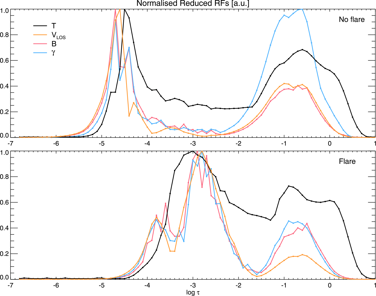
The full RF dataset has four dimensions: spatial position (Y, 830 pixels), optical depth (81 points in $\log\tau$ ), wavelength (36 samples across the two spectral lines), and the four Stokes parameters. Direct visualisation of such a dataset is difficult, so we followed the approach of Quintero Noda et al. (Reference Quintero Noda, Shimizu, Katsukawa, de la Cruz Rodríguez, Carlsson, Anan, Oba, Ichimoto and Suematsu2017) by computing an equivalent 1D RF or sensitivity function. Specifically, for each optical depth, we extracted the maximum RF value across all wavelengths and Stokes parameters, collapsing the $(\log\tau, \lambda, 4)$ domain into a 1D function of optical depth (Figure 3).

Figure 3.

Example of response functions for temperature, LOS velocity, field strength, and inclination inside (bottom) and outside (top) the flare ribbon. Reproduced from Ferrente et al. (Reference Ferrente, Quintero Noda, Zuccarello and Guglielmino2024), $\unicode{x00A9}$ The Authors, CC BY 4.0.

Figure 3 Long description

Two line graphs compare response functions for temperature, line-of-sight velocity, magnetic field strength, and inclination during a flare and no flare. Panel A: The top graph shows response functions outside the flare ribbon. The x-axis is labeled 'log τ' ranging from -7 to 1, and the y-axis is labeled 'Normalised Reduced RFs [a.u.]' ranging from 0 to 1. The black line represents temperature, the orange line represents line-of-sight velocity, the red line represents magnetic field strength, and the blue line represents inclination. Panel B: The bottom graph shows response functions inside the flare ribbon. The x-axis and y-axis labels are the same as in Panel A. The black line represents temperature, the orange line represents line-of-sight velocity, the red line represents magnetic field strength, and the blue line represents inclination.

For the Ca <sc>ii</sc> line, the maximum sensitivity within the flare ribbon occurs at deeper layers than in a standard quiet-Sun atmosphere. This indicates that strong temperature enhancements, large velocities, and concentrated magnetic fields alter the line’s formation height. In contrast, no such shift is observed for the Fe <sc>i</sc> line, consistent with the Ca <sc>ii</sc> profiles exhibiting strong emission while the photospheric line retains its typical appearance.

To determine the height of maximum sensitivity in the upper atmosphere, we identified the chromospheric peak of each atmospheric parameter. Figure 4 presents the vertical stratification along the selected cut, as well as the height of the maximum sensitivity for the region outlined with a dashed line in Figure 2. Outside the flare ribbon (Y = [0, 20] arcsec), the sensitivity peak is located around $\log\tau \sim -5$ ; whereas, within the ribbon, it shifts to deeper layers, coinciding with regions of enhanced temperature and strong LOS velocities. This suggests a reduced sensitivity to parameter variations in the upper layers of the flare ribbon; for example, LOS velocity fluctuations around $\log\tau \sim -5.5$ at Y = [20, 40] arcsec and Y = [55, 65] arcsec should be interpreted with caution.

Figure 4.

Height stratification of the atmospheric parameters for the region outlined by the dashed line in Figure 2. From top to bottom, the panels display the temperature, LOS velocity, magnetic field strength, and magnetic field inclination. In each panel, the solid line marks the height where the sensitivity to variations in the atmospheric parameters is highest for the Ca II line. Reproduced from Ferrente et al. (Reference Ferrente, Quintero Noda, Zuccarello and Guglielmino2024), $\unicode{x00A9}$ The Authors, CC BY 4.0.

2.4. Temporal evolution

We analysed the temporal evolution of the atmospheric parameters by inverting all snapshots with DeSIRe, aiming for a cadence of 10 minutes. Missing snapshots were replaced by the closest in time, and the FOV was reduced from 75 $\times$ 35 arcsec $^2$ to 50 $\times$ 35 arcsec $^2$ to reduce computation time. The two lines were inverted simultaneously using the same configuration as in the first frame.

Based on previous response function analysis, we focused on $\log\tau = -4$ outside the ribbon and $\log\tau = -3$ within it, as the height of maximum sensitivity in flaring regions shifts to deeper layers (Figure 5). Computing the exact maximum RF for each pixel at every snapshot is left for future work.

Figure 5.

Temporal evolution of T, $v_{\mathrm{LOS}}$ , B, and $\gamma$ at $\log\tau=-3$ within the flare ribbon ad at $\log\tau=-4$ outside the flare ribbon.

Figure 5 Long description

Panel A: Four heat maps show temperature evolution over time, with color gradients from dark red to bright yellow indicating temperature changes. The x-axis ranges from 0 to 30 arcseconds, and the y-axis ranges from 20 to 60 arcseconds. Green contours highlight specific regions. Panel B: Four heat maps display line-of-sight velocity changes, with color gradients from blue to red indicating velocity variations. The axes are the same as in Panel A, and black contours mark specific regions. Panel C: Four grayscale images illustrate magnetic field strength, with darker areas indicating higher field strength. Orange contours highlight specific regions. Panel D: Four heat maps show inclination changes, with color gradients from blue to red indicating inclination variations. The axes are the same as in previous panels, and black contours mark specific regions.

Within the flare ribbon, the temperature reaches 8000–9000 K after the flare peak and gradually decreases. LOS velocity maps show persistent chromospheric upflows ( $v_{\mathrm{LOS}}<0$ ) confined to the ribbons, with a shrinking spatial extent. The magnetic field strength reaches up to 1.4 kG in hot areas, becoming more fragmented during the decay, while magnetic inclination remains mostly vertical with no abrupt changes throughout the post-flare evolution.