2 Problem formulation

We are interested in examining the dynamic behaviour of an encapsulated microbubble with initial radius $R_{0}^{\prime }$ that is submerged in a Newtonian liquid of density $\unicode[STIX]{x1D70C}$ and dynamic viscosity $\unicode[STIX]{x1D707}$ when the full viscous effects of the surrounding fluid are accounted for. We consider an unbounded flow and we investigate the bubble’s response to a disturbance imposed on the far pressure field:

with $P_{st}^{\prime }$ , $P_{dist}^{\prime }$ denoting the dimensional undisturbed and disturbed pressure on the far field, respectively. A step change disturbance is introduced:

where $\unicode[STIX]{x1D700}$ represents the magnitude of the imposed disturbance; throughout this paper dimensional variables are indicated by primed letters.

The initial radius $R_{0}$ of the bubble is taken as the characteristic length scale of the problem, whereas the angular eigenfrequency $\unicode[STIX]{x1D714}_{0}$ pertaining to radial pulsations of the bubble determines the appropriate time scale as $1/\unicode[STIX]{x1D714}_{0}$ . Throughout this paper the Mooney–Rivlin law is used for the elastic part of the shell stresses which describes materials that are very thin, isotropic, volume-incompressible and have a strain-softening behaviour, i.e. the shear modulus of the membrane is reduced as strain grows. The angular eigenfrequency of the breathing mode $\unicode[STIX]{x1D714}_{0}$ for a coated microbubble as obtained by linear stability analysis reads:

where $\unicode[STIX]{x1D70E}$ is the surface tension, $\unicode[STIX]{x1D712}$ the area dilatational modulus and $\unicode[STIX]{x1D6FE}$ the polytropic constant. Due to the small size of such microbubbles their eigenfrequency for volume pulsations is of the order of several MHz. As a result, and in order to facilitate comparison of results obtained with different area dilatation moduli, in the present study we use the angular frequency, $\unicode[STIX]{x1D714}_{r}$ , of a conventional gas bubble with the same properties as those associated with the coated microbubble under examination, except for the area dilatation modulus, which is set to 0, as the reference time scale of the problem; it reads as $\unicode[STIX]{x1D714}_{r}=2\unicode[STIX]{x03C0}\unicode[STIX]{x1D708}_{r}$ , with $\unicode[STIX]{x1D708}_{r}$ set to 1 MHz. Therefore, the characteristic velocity and pressure scales are $\unicode[STIX]{x1D714}_{r}R_{0}$ and $\unicode[STIX]{x1D70C}\unicode[STIX]{x1D714}_{r}^{2}R_{0}^{2}$ , respectively.

The problem of a single bubble in an unbounded flow is described via a spherical coordinate system and in order to obtain the governing equations we assume axisymmetric variations of the bubble shape as well as the liquid velocity and pressure, i.e. no variations are considered in the azimuthal direction for either the liquid or the bubble. In figure 1 a schematic representation of the flow under consideration is provided, with $f_{1}$ denoting the $r$ -coordinate of the thin shell that coats the bubble.

Figure 1.

Single bubble in an unbounded flow.

The flow in the surrounding liquid is governed by the mass conservation and momentum equations. The liquid is taken to be incompressible, in which case the continuity equation and momentum balance, via the Navier–Stokes equations, read in dimensionless form:

where $\boldsymbol{u}=(u_{r},u_{\unicode[STIX]{x1D703}},0)$ , $Re=(\unicode[STIX]{x1D70C}\unicode[STIX]{x1D714}_{r}R_{0}^{2})/\unicode[STIX]{x1D707}$ is the Reynolds number of the surrounding liquid flow that compares inertia with viscous forces, $\unicode[STIX]{x1D748},\unicode[STIX]{x1D749}$ , the full and deviatoric stress tensors in the surrounding fluid and $\unicode[STIX]{x1D644}$ the unit tensor. In the above formulation buoyancy has been neglected owing to the small size of the bubble.

In order to obtain the deformation of the bubble we use a Lagrangian representation of the interface by introducing a Lagrangian coordinate $\unicode[STIX]{x1D709}\,(0\leqslant \unicode[STIX]{x1D709}\leqslant 1)$ which identifies the particles on the interface. In this context, the arclength, $S$ , of the interface is related to the coordinate, $\unicode[STIX]{x1D709}$ , of the interface by:

The force balance on the gas–liquid interface reads in dimensionless form:

where $\boldsymbol{n}$ denotes the unit normal vector pointing towards the surrounding fluid and $\unicode[STIX]{x1D644}$ , $\unicode[STIX]{x1D749}_{l}$ the unit and deviatoric stress tensors of the liquid, respectively; $P_{G}$ is the dimensionless pressure of the gas inside the bubble; $\unicode[STIX]{x1D735}_{s},k_{m}$ denote the surface gradient and mean curvature of the bubble’s interface, respectively, and $We=(\unicode[STIX]{x1D70C}\unicode[STIX]{x1D714}_{r}^{2}R_{0}^{3})/\unicode[STIX]{x1D70E}$ is the Weber number comparing inertia with capillary forces. Despite its viscoelastic nature a certain amount of surface tension is typically assumed for the shell (Church Reference Church1995; Khismatullin & Nadim Reference Khismatullin and Nadim2002; Marmottant et al. Reference Marmottant, van der Meer, Emmer, Versluis, de Jong, Hilgenfeldt and Lohse2005; Sarkar et al. Reference Sarkar, Shi, Chatterjee and Forsberg2005) as a measure of the isotropic surface tension. Finally, $\unicode[STIX]{x1D71F}\boldsymbol{F}$ is the resultant force due to the viscoelastic properties of the membrane, which is set to zero in the case of a gas-filled bubble. Based on the theory of elastic shells the force, $\unicode[STIX]{x1D71F}\boldsymbol{F}$ , in the case of a contrast agent is derived by the surface divergence of the viscoelastic tension tensor on the membrane’s surface and is equal to:

with $\unicode[STIX]{x1D70F}_{s},\unicode[STIX]{x1D70F}_{\unicode[STIX]{x1D719}}$ denoting the principal elastic tensions, $r_{0}=r\sin \unicode[STIX]{x1D703}$ the radial polar coordinate and $\boldsymbol{e}_{s}$ the tangential unit vector; $q$ is the transverse shear tension that is obtained from a torque balance on the shell (Timoshenko & Woinowsky-Krieger Reference Timoshenko and Woinowsky-Krieger1959; Pozrikidis Reference Pozrikidis2001):

where $m_{s},m_{\unicode[STIX]{x1D719}}$ are the principal bending moments. The membrane and bending stresses are defined via the shell constitutive laws. The membrane tensions consist of an elastic and a viscous component, e.g.  $\unicode[STIX]{x1D70F}_{s}=\unicode[STIX]{x1D70F}_{s,el}+\unicode[STIX]{x1D70F}_{s,v}$ . We adopt the Mooney–Rivlin model for the elastic part (Barthes-Biesel, Diaz & Dhenin Reference Barthes-Biesel, Diaz and Dhenin2002):

with $\unicode[STIX]{x1D706}_{s},\unicode[STIX]{x1D706}_{\unicode[STIX]{x1D719}}$ denoting the principal extension ratios and $b$ is the degree of softness. In axisymmetric geometry they assume the form:

The viscous components of the in-plane stresses, $\unicode[STIX]{x1D70F}_{s,v},\unicode[STIX]{x1D70F}_{\unicode[STIX]{x1D719},v}$ , are provided via introduction of a Newtonian-like linear constitutive law while taking the dilatational and shear viscosity of the shell as equal (Barthes-Biesel & Sgaier Reference Barthes-Biesel and Sgaier1985) to $\unicode[STIX]{x1D707}_{s}$ , in the absence of more accurate rheological data. In dimensionless form this reads:

with $(1/\unicode[STIX]{x1D706}_{s})(\unicode[STIX]{x2202}\unicode[STIX]{x1D706}_{s}/\unicode[STIX]{x2202}t)$ and $(1/\unicode[STIX]{x1D706}_{\unicode[STIX]{x1D711}})(\unicode[STIX]{x2202}\unicode[STIX]{x1D706}_{\unicode[STIX]{x1D711}}/\unicode[STIX]{x2202}t)$ denoting the principal components of the rate of deformation tensor and $Re_{s}$ the shell Reynolds number defined as $Re_{s}=(\unicode[STIX]{x1D70C}_{l}\unicode[STIX]{x1D714}_{r}R_{0}^{3})/\unicode[STIX]{x1D707}_{s}$ .

Finally, the dimensionless principal bending moments $m_{s}$ , $m_{\unicode[STIX]{x1D719}}$ are provided by the following equations that constitute a linear constitutive law for the bending stresses:

where $\unicode[STIX]{x1D708}$ is Poisson’s ratio, $k_{b}$ is the bending elasticity and $K_{s},K_{\unicode[STIX]{x1D719}}$ the bending measures of strain that relate the deviation of the two principal curvatures $k_{s},k_{\unicode[STIX]{x1D719}}$ from their reference value $k_{s}^{R},k_{\unicode[STIX]{x1D719}}^{R}$ in the absence of bending:

Bending resistance $k_{b}$ is treated as an independent parameter herein, in order to account for the fact that a definitive shell thickness cannot be defined for phospholipid shells (Zarda, Chien & Skalak Reference Zarda, Chien and Skalak1977), while the reference curvatures are taken to be equal and constant, corresponding to a spherical reference shape. A more detailed description of the approach presented above for the modelling of the viscoelastic shell of the bubble can be found in Tsiglifis & Pelekasis (Reference Tsiglifis and Pelekasis2008, Reference Tsiglifis and Pelekasis2011, Reference Tsiglifis and Pelekasis2013).

Continuity of the liquid and shell velocities on the interface reads as:

with $\boldsymbol{r}=r\boldsymbol{e}_{r}$ denoting the position vector of a particle at the interface. At equilibrium a stress-free state is assumed on the interface of radius $R_{0}$ , where the dimensionless pressure, $P_{G}$ , inside the bubble is related to the dimensionless pressure, $P_{st}$ , on the far field through the Young–Laplace equation:

The pressure inside the bubble is taken to be uniform due to negligible density and kinematic viscosity of the enclosed gas. Moreover, heat transfer between the bubble and the surrounding liquid is assumed to take place fast in comparison with the time scale of the phenomena under consideration. In this context, bubble’s oscillations are characterized as nearly isothermal, and therefore the bubble pressure is given by:

with $V_{G}$ denoting the dimensionless instantaneous volume of the bubble, $V_{G}(t=0)=4\unicode[STIX]{x03C0}/3$ the initial volume of the bubble and $\unicode[STIX]{x1D6FE}$ the polytropic constant set to 1.07 for an almost isothermal variation. The latter value is also close to the ratio between the specific heats of certain ideal gases that are carried by known contrast agents and undergo adiabatic pulsations during insonation.

Finally, in appendix A the analysis of the energy conservation is presented and the different energy constituents are extracted in order to illustrate the manner in which the energy is distributed during the evolution of the phenomena under consideration.

3 Numerical methodology

Numerical solution of the above problem formulation is performed via the Galerkin Finite Element Methodology with a hybrid scheme that uses 2D Lagrangian functions to discretize the surrounding flow field, in conjunction with 1D cubic splines for the bubble shape. In the case of an encapsulated bubble the introduction of cubic splines is necessary because a fourth-order derivative arises in the force balance equation through the bending resistance of the membrane. They are preferred over other functions, such as the Hermite cubic functions, because they ensure continuity of the second derivative without introducing the derivative of the interpolated function as an additional unknown to the problem. In this context, biquadratic and bilinear Lagrangian basis functions are used for the velocity and the pressure of the liquid respectively, while cubic spline functions are employed to discretize the interface. Pressure is treated via a staggered grid formulation in order to circumvent the Babuska–Brezzi condition and avoid numerical instabilities (Babuska Reference Babuska1973). The fully implicit Euler time integration scheme is introduced in order to make optimal use of its numerical dissipation properties against growth of short-wave instabilities. In this context, the discretized forms of continuity and Navier–Stokes equations are:

where $M_{i},N_{i}$ are the biquadratic and bilinear Lagrangian functions respectively; $\text{d}V=r^{2}\sin \unicode[STIX]{x1D703}\,\text{d}r\,\text{d}\unicode[STIX]{x1D703}\,\text{d}\unicode[STIX]{x1D719}$ is the differential volume of integration and vector $\boldsymbol{e}_{\boldsymbol{k}}$ refers to one of the unit vectors $\boldsymbol{e}_{\boldsymbol{r}},\boldsymbol{e}_{\unicode[STIX]{x1D73D}}$ corresponding to the components of the momentum differential balance. Upon integrating by parts (3.2), the $r$ - and $\unicode[STIX]{x1D703}$ -components of the weak formulation of the momentum equation are derived:

The azimuthal angle, $\unicode[STIX]{x1D711}$ , has been integrated out of the above equations due to axisymmetry, essentially generating a two-dimensional geometry to be discretized with a line integral at its boundary. The area integral corresponds to the region between the bubble–liquid interface and the far field, and the line integral is defined along the generating curve of the axisymmetric shell and a circular surface in the far field where the pressure disturbance is applied.

The usual procedure when simulating flow problems with the Finite Element Methodology technique is to substitute for quantities appearing in the line integrals with their equivalent terms arising from the normal and tangential force balance equations. This procedure is appropriate for the study of free bubbles. However, in the case of contrast agents this is impossible since that particular integral requires interpolation of a fourth-order partial derivative for the calculation of bending stresses, and Lagrangian basis functions, $M_{i}$ , fail to interpolate the second derivatives that arise in the weak formulation after integration by parts. Therefore the momentum equation is not written on the interface. Rather, continuity of the radial and polar velocity components is imposed as an essential condition. Furthermore, since we employ a Lagrangian representation for the shape of the bubble we need two equations for each particle, $\unicode[STIX]{x1D709}$ , to determine the two coordinates $r(\unicode[STIX]{x1D709},t)$ and $\unicode[STIX]{x1D703}(\unicode[STIX]{x1D709},t)$ . For this reason the normal and tangential force balances are employed and are discretized using the one-dimensional cubic splines as basis functions $B_{i}$ :

where the integration length is defined as 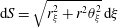$\text{d}S=\sqrt{r_{\unicode[STIX]{x1D709}}^{2}+r^{2}\unicode[STIX]{x1D703}_{\unicode[STIX]{x1D709}}^{2}}\,\text{d}\unicode[STIX]{x1D709}$ in terms of the Lagrangian variable $\unicode[STIX]{x1D709}$ . On the opposite end of the flow domain, i.e. the far field, the imposed pressure disturbance is prescribed on the right-hand side of the radial component of the momentum balance. This is a superparametric interpolation scheme for capturing the position of the interface that has also been used elsewhere in the context of free surface problems (Saito & Scriven Reference Saito and Scriven1981; Kistler & Scriven Reference Kistler, Scriven, Pearson and Richardson1983). Details pertaining to the efficiency of $B$ -cubic splines as basis functions in flow problems involving free surfaces are provided in Pelekasis, Tsamopoulos & Manolis (Reference Pelekasis, Tsamopoulos and Manolis1992).

For the grid construction we use and compare two different methods: the spine method and the elliptic mesh generation technique. Both of them are described in detail in appendix B.

The nonlinearity of the problem is treated with the Newton–Raphson method and the following linear system of equations is solved during each iteration:

with $\boldsymbol{R}$ denoting the residual vector, $\text{d}\boldsymbol{C}$ the vector of the unknowns and $\unicode[STIX]{x1D645}$ the Jacobian matrix of the system. Vector $\text{d}\boldsymbol{C}$ includes the two components of the velocity and the pressure of the liquid, the gas pressure and the shape of the bubble. The Jacobian matrix, $\unicode[STIX]{x1D645}$ , contains the finite element discretization of the momentum and continuity equations (3.1), (3.2), where the fully implicit Euler time integration scheme is implemented, along with the tangential and normal force balances at the interface, equations (3.4), and the isothermal law for the pressure variation in the bubble, equation (2.17). In this fashion, the Jacobian matrix assumes the form of an arrow with the gas pressure and the bubble shape occupying the arrow columns. A separate Newton–Raphson iterative procedure follows the above time integration process within each time step, for the implementation of the elliptic mesh generation scheme and the construction of the updated grid. Despite the fact that in previous numerical studies of the nonlinear dynamic response of liquid drops and bridges (Chen & Tsamopoulos Reference Chen and Tsamopoulos1993; Patzek et al. Reference Patzek, Basaran, Benner and Scriven1995; Notz & Basaran Reference Notz and Basaran1999, Reference Notz and Basaran2004) the trapezoid rule is implemented in the context of a predictor–corrector time integration scheme, in the present study we employ the fully implicit Euler method in order to make use of its inherent damping properties against growth of spurious shape modes. This approach by no means compromised the accuracy of the solution, as was verified by extensive tests with varying time step and continuous monitoring of the energy.

In order to reduce computational time we have chosen to solve the problem iteratively with the GMRES (Generalized Minimum Residual) (Saad & Schultz Reference Saad and Schultz1986) rather than a direct method. GMRES is an iterative method and therefore is more effective when the matrix to be inverted does not contain zero diagonal elements (Elman, Silvester & Wathen Reference Elman, Silvester and Wathen2005). In the problems examined herein this approach does not apply, and consequently the GMRES method with right or left preconditioning is employed. The preconditioning is performed using Incomplete Lower Upper (ILU) factorization. ILU is based on Gauss elimination in order to eliminate certain elements of the matrix in specific positions outside the main diagonal (Saad Reference Saad1996). The implementation of ILU and GMRES is performed using the SPARSKIT software (Saad Reference Saad1996). It is the experience of the authors that the use of GMRES reduces computational time dramatically, and indeed that was seen to be the case in the present study as well. As an extra effort to further reduce computational time we avoid construction and ILU factorization of the Jacobian matrix in every time step. The number of time steps over which the Jacobian matrix can remain unaltered without compromising the efficiency of the algorithm depends strongly on the intensity of the shape deformation of the bubble, and was seen to vary considerably between 1 and 500 time steps.

4 Results and discussion

In this section we present an extensive parametric study in our effort to capture the dynamics of coated microbubbles in response to a step change in the far-field pressure, until static equilibrium is achieved. Previous static and stability analysis for both polymeric and the softer phospholipid shells (Tsiglifis & Pelekasis Reference Tsiglifis and Pelekasis2011; Lytra & Pelekasis Reference Lytra and Pelekasis2014) predict the onset of a bifurcating branch that is characterized by symmetric or asymmetric shapes when static buckling first occurs, depending on the area dilatation modulus, $\unicode[STIX]{x1D712}$ , of the shell. In particular, for relatively smaller values of the area dilatation modulus, static buckling favours asymmetric shapes that are indented in one of the two poles where bending stresses develop in an effort to relieve the shell from the excess energy due to compressive stresses. In contrast, as it increases, symmetric shapes emerge in the post-buckling state where a local indentation at both poles arises. Such a static arrangement facilitates the development of bending stresses in a larger portion of the shell, as a means to alleviate the intense straining of compressed spherical shells characterized by a large area dilatation modulus. This pattern is particularly true for phospholipid shells (they are the focus of the present study) that obey the Mooney–Rivlin constitutive law and become even harder at compression. The crucial parameter that determines the onset of buckling is the stiffness ratio between bending and dilatation, $k_{b}/(\unicode[STIX]{x1D712}R_{0}^{2})=(\unicode[STIX]{x1D6FF}/3/R_{0})^{2}$ when $\unicode[STIX]{x1D708}=0.5$ , with $\unicode[STIX]{x1D6FF}$ denoting the shell thickness and $\unicode[STIX]{x1D708}$ the Poisson ratio. Furthermore, the resistance to compression is an additional factor that affects the static and dynamic response of phospholipid shells, in comparison with the hard polymeric ones, as will be seen from the analysis of the results that follows based on the relative volume compression to area dilatation stiffness, $P_{St}R_{0}/\unicode[STIX]{x1D712}$ . The dynamic pattern towards the static equilibrium is of interest as a function of the shell parameters in the presence of viscous dissipation in the surrounding liquid, in view of the fact that static equilibrium was not captured in the context of boundary element dynamic simulations presented in Tsiglifis & Pelekasis (Reference Tsiglifis and Pelekasis2013). In particular, we are interested in investigating the possibility that the above static shapes be anticipated by finite time singularities that are typically observed with gas bubbles such as jet formation and breakup.

The phospholipid shell that was studied in the benchmark calculation presented in the previous section is simulated, setting the area dilatation modulus and imposing a series of step change disturbances, in order to study the dynamic evolution of the shell shape towards static equilibrium. For this particular set of parameters, setting area dilatation modulus $\unicode[STIX]{x1D712}$ to $0.12~\text{N}~\text{m}^{-1}$ , static stability analysis records two non-spherical bifurcating branches, off the main branch of compressed spherical shells, dominated by symmetric and asymmetric $\text{P}_{2}$ and $\text{P}_{3}$ modes, respectively. The first one emerges at the critical value of $\unicode[STIX]{x1D700}=1.65$ , whereas the critical threshold for the asymmetric branch is $\unicode[STIX]{x1D700}=1.78$ (Lytra & Pelekasis Reference Lytra and Pelekasis2014). Our dynamic simulations verify that the threshold in step change for static buckling to occur is 1.65. Moreover, as was also reported in § 3.1 that was dedicated to benchmarking, below this threshold it was not possible to capture any deformed shapes at static equilibrium irrespective of the initial shape disturbance that was applied on the compressed spherical shape obtained for a certain step change in pressure. In particular, the eigenvector obtained at criticality was superimposed on the compressed spherical shape in the form of an initial shape imperfection with increasing amplitude, $r=R+\unicode[STIX]{x1D700}F(\unicode[STIX]{x1D709})$ . $F(\unicode[STIX]{x1D709})$ denotes the eigenvector corresponding to the eigenvalue that first turns unstable at criticality (see also Lytra & Pelekasis (Reference Lytra and Pelekasis2014)), and contains all the characteristics of the solution family that bifurcates from the main spherical branch at the buckling threshold. In all cases the shell eventually returned to the spherical configuration, thus verifying the subcritical nature of the bifurcation. In contrast, when the initial step change in pressure exceeded the critical buckling threshold value, the coated bubble was seen to eventually reach a non-spherical static equilibrium, even in the absence of an initial shape disturbance.

This behaviour is in marked contrast with the dynamic response of polymeric shells in the neighbourhood of the bifurcation point (figure 5 in Tsiglifis & Pelekasis (Reference Tsiglifis and Pelekasis2013)). In the latter case static stability predicts that an asymmetric eigenmode, $\text{P}_{11}$ , dominates the post-buckling behaviour, followed by a symmetric bifurcation characterized by $\text{P}_{12}$ . Nevertheless, dynamic simulations with the boundary integral method as well as with the present finite element methodology do not recover the spherical shape or the primary bifurcation branch for perturbations below or above the bifurcation point, respectively. Rather they indicate a continuous evolution of the shape that is conjectured to lead to breakup or to the formation of contact regions. In the present study it will be seen that phospholipid shells exhibit a different response pattern leading to deformed shapes of different intensity depending on the magnitude of the step change in the far-field pressure. As the latter is further increased, static shapes exhibiting contact are captured by the dynamic simulations rather than jet formation or breakup.

Figure 8.

(a) Temporal evolution of bubble shape and (b) temporal evolution of radius and shape mode decomposition for a contrast agent ( $R=3.6~\unicode[STIX]{x03BC}\text{m}$ , $\unicode[STIX]{x1D707}_{s}=20~\text{Pa}~\text{s}$ , $\text{thickness}=1~\text{nm}$ , $\unicode[STIX]{x1D712}=0.12~\text{N}~\text{m}^{-1}$ , $k_{b}=3\times 10^{-14}~\text{N}~\text{m}$ ) for a step change disturbance ( $\unicode[STIX]{x1D700}=2$ ) with the spine method. (c) Total energy variation, (d) viscous versus shell damping and (e) distribution among different forms of energy as a function of time.

Figure 9.

(a) Temporal evolution of bubble shape and (b) temporal evolution of radius and shape mode decomposition for a contrast agent ( $R=3.6~\unicode[STIX]{x03BC}\text{m}$ , $\unicode[STIX]{x1D707}_{s}=20~\text{Pa}~\text{s}$ , $\text{thickness}=1~\text{nm}$ , $\unicode[STIX]{x1D712}=0.12~\text{N}~\text{m}^{-1}$ , $k_{b}=3\times 10^{-14}~\text{N}~\text{m}$ ) for a step change disturbance ( $\unicode[STIX]{x1D700}=2$ ) with the elliptic mesh method. (c) Total energy variation, (d) viscous versus shell damping and (e) distribution among different forms of energy as a function of time.

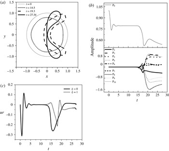
Figures 8 and 9 illustrate the rich bifurcation structure that is produced in the post-buckling, or supercritical, regime in terms of the amplitude $\unicode[STIX]{x1D700}$ of the step change in the far-field pressure. In both cases $\unicode[STIX]{x1D700}$ is set to 2, which is above the buckling threshold, with the spine and elliptic mesh generation procedures implemented in figures 8 and 9, respectively. Both are valid and numerically converged static equilibrium shapes, and represent possible alternative static configurations to the spherical shape for the same external overpressure. The shape evolution of the coated bubble until static equilibrium is established is shown in figure 8(a), captured via the spine method, indicating the onset of a symmetric oblate static shape that exhibits indentations in an extended region around the two poles. As a result of the strain-softening nature of the Mooney–Rivlin shell it becomes harder at compression, and consequently an indentation starts to develop in the pole region as a means to relieve the shell from the large in-plane stresses, via bending. This can be gleaned from figure 8(b), illustrating the Legendre mode decomposition of the bubble shape. The breathing mode $\text{P}_{0}$ in particular exhibits a first plateau, after a short oscillatory phase with its natural angular frequency $\unicode[STIX]{x1D714}_{0}$ , corresponding to the compressed spherical shape in response to the step change in pressure $(R=0.8022)$ . Subsequently buckling takes place, and energy is distributed among different shape modes until the shell settles to a symmetrically deformed state dominated by $\text{P}_{2}$ and $\text{P}_{4}$ in figure 8(b).

It should be stressed that, during the transient phase between the compressed spherical state and the final static shape, asymmetric modes emerge, most notably $\text{P}_{3}$ as can be gleaned from the mode decomposition shown in figure 8(b) and the corresponding shapes in figure 8(a), indicating the possibility for asymmetrically deformed static shapes to develop. Indeed, asymmetric static shapes are also possible for the same parameter values. Nevertheless, the symmetric configuration prevails at static equilibrium owing to its comparatively smaller total energy, as shown in figure 8(c), depicting the evolution of the total shell energy. The energy variation follows a similar pattern as the breathing mode $\text{P}_{0}$ with the initially elevated energy content, attributed to surface energy and internal/external pressure level, gradually dissipated predominantly by the action of shell viscosity; see also figure 8(d), presenting the shell and liquid components of viscous dissipation during the entire process. In this fashion, the shell goes through a local energy minimum corresponding to a compressed sphere, which is further destabilized to acquire the final symmetric shape with the slight indentation at the two poles. At this point it should be stressed that, despite the fact that based on static analysis (Lytra & Pelekasis Reference Lytra and Pelekasis2014) the spherical shape was found to be favoured energetically over all deformed shapes in the post-buckling regime, simulations performed herein show that, when the surrounding liquid is included in the total energy balance, deformed shapes that exhibit significant volume compression ( $V/V_{0}=0.47$ versus 0.516 for the compressed sphere) at static equilibrium acquire lower energy levels than the equivalent spherical ones obtained for the same step change in the external pressure, and as a result dominate static equilibrium. This is clearly illustrated in figure 8(c) and is a recurring theme in the present study. The decomposition of energy among various forms is shown in figure 8(e), where the importance of bending and surface energy in redistributing the shell energy due to stretching and compression, thus leading to energy minimum, is illustrated.

Figure 9(a) depicts the dynamic pattern of shape deformation of a microbubble subject to the same disturbance as in figure 8, as obtained with the elliptic mesh generation technique. The response pattern is similar with the difference that now prolate shapes are obtained at static equilibrium. This is an equally valid and numerically converged static solution belonging to a different bifurcation branch that is achieved instead of the oblate shapes as a result of the different numerical attributes of the elliptic mesh generation scheme. This is verified independently from the above dynamic simulations in the context of static analysis and is a manifestation of the rich bifurcation diagram of coated microbubbles. As in figure 8, an intermediate spherical state is obtained with the shell being uniformly compressed, in figure 9(b), that is further destabilized in order to release the excess elastic energy it has acquired as a result of shell hardening during compression, by redistributing it along the interface or by converting it to bending energy. In this simulation it is also the case that the second Legendre mode dominates, with $\text{P}_{3}$ and the rest of the asymmetric modes remaining negligibly small while $\text{P}_{4}$ and the rest of the symmetric modes gradually grow due to nonlinearity (figure 9 b). Eventually a symmetrically deformed static shape emerges that is prolate along the axis of symmetry. This shape is also characterized by more severe volume compression, $V/V_{0}=0.51$ versus 0.516 for the spherical shape, and consequently smaller energy content than the uniformly compressed shell (figure 9 c). This static equilibrium shape constitutes an alternative arrangement at static equilibrium, for the same parameter range, that is a result of the additional degrees of freedom offered by shell elasticity to the microbubble’s dynamics. Throughout the above-described dynamic process, energy is dissipated mainly due to shell viscosity that dominates liquid viscosity (figure 9 d), especially during compression. The prolate shape obtained in this case does not exhibit significant bending (figure 9 a,e), owing to the relatively large bending stiffness, $k_{b}/(\unicode[STIX]{x1D712}R_{0}^{2})\approx 0.02$ , and hence the lack of indentations. Bending of the shell at the equator is not as effective in reducing shell energy since it basically affects in-plane stresses in the polar direction, whereas bending around the poles uniformly affects in-plane stresses along both the polar and azimuthal directions. Hence, among the two symmetric static configurations, the one with the oblate shape is more stable in the sense that its energy content is lower. It should also be stressed that the pattern of prolate versus oblate shapes was not seen in static calculations of coated bubbles obtained in previous studies (Knoche & Kierfeld Reference Knoche and Kierfeld2011; Lytra & Pelekasis Reference Lytra and Pelekasis2014). This is attributed to the relatively larger value of the relative stiffness ratio, $k_{b}/(\unicode[STIX]{x1D712}R_{0}^{2})\approx 0.02$ for the parameter range relevant to the simulations shown in figures 8 and 9, that makes bending an energy consuming alternative to stretching, thus affording the onset of stable prolate shapes in the post-buckling regime.

Upon increasing the amplitude of the external disturbance $(\unicode[STIX]{x1D700}=3)$ the spine method fails to capture the evolution of the interface. In contrast, the elliptic mesh generation technique (figure 10), captures the time evolution of the dynamic response until static equilibrium. The final static shape is a symmetric oblate one with two indentations in the region around the two poles. It is essentially a continuation of the static arrangement produced by the spine method when $\unicode[STIX]{x1D700}=2$ (see also figure 8), that proceeds further along the bifurcation branch pertaining to oblate shapes. It constitutes the preferred static arrangement owing to its lower energy content in comparison with the prolate shapes.

Figure 10.

(a) Temporal evolution of bubble shape and (b) temporal evolution of shape mode decomposition for a contrast agent ( $R=3.6~\unicode[STIX]{x03BC}\text{m}$ , $\unicode[STIX]{x1D707}_{s}=20~\text{Pa}~\text{s}$ , $\text{thickness}=1~\text{nm}$ , $\unicode[STIX]{x1D712}=0.12~\text{N}~\text{m}^{-1}$ , $k_{b}=3\times 10^{-14}~\text{N}~\text{m}$ ) for a step change disturbance $(\unicode[STIX]{x1D700}=3)$ with the elliptic mesh method. (c) Grid generated via the elliptic mesh generation technique. (d) Total energy variation and (e) distribution among different forms of energy as a function of time. (f) Time evolution of $\text{P}_{1}$ and (g) time evolution of shape mode decomposition when the origin of the coordinate system is moved.

The shape and mode decomposition in this case are provided in figure 10(a,b). Figure 10(c) depicts the computational grid produced by the elliptic mesh generation technique as the indentation around the two poles develops. The increased area of the elements near the two indentations is evident, indicating the relatively larger error in these two areas. The fashion in which static equilibrium is approached should also be noted, as the shell temporarily acquires asymmetric shapes dominated by $\text{P}_{3}$ and $\text{P}_{5}$ , marking the existence of an additional asymmetric branch with a single indentation at the north pole; see also the time evolution of the microbubble shapes shown in figure 8(a), obtained with the spine method when $\unicode[STIX]{x1D700}=2$ . Nevertheless, here also the oblate symmetric shape eventually prevails due to its lower energy content (figure 10 d). The pattern of shell damping dissipating the kinetic energy by relaxing the compressive stresses persists in this case also (figure 10 e). Eventually, the shell acquires its static arrangement with bending stresses developing at the expense of strain.

Another important aspect of this simulation pertains to the gradual emergence of a translational motion of the microbubble’s centre of mass that can also be observed by careful inspection of figure 10(a). This is a result of nonlinear interaction between emerging consecutive shape modes, $\text{P}_{n}$ and $\text{P}_{n+1}$ , that can also explain the persistence of $\text{P}_{3}$ and $\text{P}_{5}$ in the symmetric static shape whose centre of mass is clearly displaced from its original position at the origin of the coordinate system. The displacement is more severe in comparison with the situation shown in figure 8(a) due to the smaller initial disturbance in the latter case (see also figure 10(f) illustrating the time evolution of $\text{P}_{1}$ ). Upon moving the origin of the coordinate system to the midpoint between the two poles (figure 10 g), the same symmetric static shape is obtained while the odd modes are removed from the Legendre decomposition of the shape.

As the intensity of the step change is further increased, setting $\unicode[STIX]{x1D700}=3.5$ , the solution family of oblate shapes persists as the preferred static configuration, with the emerging shape exhibiting a contact region where the two poles meet (figure 11 a). The mode decomposition of the shell shape becomes richer in higher modes (figure 11 b), while the total energy never fully settles to a constant value (figure 11 c). In fact, as illustrated in figure 11(d), showing the evolution of the normal velocity at the north pole, the latter acquires a large speed as the indentation forms and gradually intensifies. This is a manifestation of the divergence process that takes place during the buckling event. However, the process of kinetic energy accumulation is eventually arrested mainly by the development of viscous stresses in the shell that mitigate the onset of compressive in-plane stresses. The kinetic energy of the shell as well as the energy due to compression and strain are redistributed in favour of bending and surface energy; see also figure 11(e). For large external overpressures, prolonged action of shell viscosity significantly relaxes the compressive stresses in the pole region where the indentation arises. In this process the pole region assumes an almost spherical shape as the radius of curvature progressively decreases following the volume change; see also figure 11(c–f), while bending takes place mostly around the equator.

Figure 11.

(a) Temporal evolution of bubble shape and (b) temporal evolution of shape mode decomposition for a contrast agent ( $R=3.6~\unicode[STIX]{x03BC}\text{m}$ , $\unicode[STIX]{x1D707}_{s}=20~\text{Pa}~\text{s}$ , $\text{thickness}=1~\text{nm}$ , $\unicode[STIX]{x1D712}=0.12~\text{N}~\text{m}^{-1}$ , $k_{b}=3\times 10^{-14}~\text{N}~\text{m}$ ) for a step change disturbance $(\unicode[STIX]{x1D700}=3.5)$ with the elliptic mesh method. (c) Time evolution of the total shell energy. (d) Temporal evolution of velocity at the two poles. (e) Distribution among different forms of energy and (f) viscous versus shell damping as a function of time.

Eventually contact is established in the region around the two poles, while the shell never quite achieves a static configuration, since simulations cannot proceed beyond the point of first contact. To this end, further modelling is required and is out of the scope of the present study. Rather, this is viewed as the inception of the dynamic process leading to the formation of a contact region. Thus, it is anticipated that the eventual static equilibrium will exhibit regions of contact whose length depends on the magnitude of the external overpressure, in the manner that earlier studies of the static response of hard shells (Knoche & Kierfeld Reference Knoche and Kierfeld2011) obtain shapes with progressively longer contact regions at the poles as the limiting state of solution families with post-buckling shapes. In this fashion, jet formation is avoided as it entails the onset of areas of very large curvature and speed corresponding to large bending and kinetic energy components. This is, however, prevented by the action of shell viscosity that damps kinetic energy and does not allow intensive bending or strain to develop in the pole region.

Figure 12.

(a) Temporal evolution of bubble shape and (b) temporal evolution of radius and shape mode decomposition for a contrast agent ( $R=3.6~\unicode[STIX]{x03BC}\text{m}$ , $\unicode[STIX]{x1D707}_{s}=20~\text{Pa}~\text{s}$ , $\text{thickness}=1~\text{nm}$ , $\unicode[STIX]{x1D712}=0.24~\text{N}~\text{m}$ , $k_{b}=3\times 10^{-14}~\text{N}~\text{m}$ ) for a step change disturbance ( $\unicode[STIX]{x1D700}=2$ ) with the elliptic mesh method. (c) Time evolution of the total shell energy. (d) Viscous versus shell viscosity and (e) distribution among different forms of energy as a function of time.

Next we examine a case where, according to static analysis (Tsiglifis & Pelekasis Reference Tsiglifis and Pelekasis2013; Lytra & Pelekasis Reference Lytra and Pelekasis2014), a bifurcation to an asymmetric static state emerges first in the original branch pertaining to isotropically compressed spherical shells. To this end we consider the same contrast agent as in the previous paragraphs with twice the area dilatation modulus $(\unicode[STIX]{x1D712}=0.24~\text{N}~\text{m}^{-1})$ . This microbubble is characterized by a smaller bending to stretching stiffness ratio, $k_{b}/(\unicode[STIX]{x1D712}R_{0}^{2})\approx 0.01,$ and an $O(1)$ volume compression to area dilatation stiffness ratio, $P_{St}R_{0}/\unicode[STIX]{x1D712}\approx 1.5$ . Based on static stability the buckling threshold for such a shell corresponds to a disturbance with amplitude $\unicode[STIX]{x1D700}=1.35$ and signifies the onset of an asymmetric mode, namely $\text{P}_{3}$ . As the amplitude is further increased to $\unicode[STIX]{x1D700}=1.43$ , a second bifurcation occurs that is dominated by the symmetric mode $\text{P}_{2}$ . Figure 12 provides the response pattern of a microbubble of this size and shell type to a step change disturbance with amplitude $\unicode[STIX]{x1D700}=2$ as obtained via the elliptic mesh generation technique. After the standard plateau corresponding to the compressed spherical shape the symmetric Legendre mode $\text{P}_{4}$ appears first, followed shortly by modes $\text{P}_{3}$ and $\text{P}_{2}$ . Subsequently, more modes appear as a result of nonlinear interaction. It is of great interest that shortly after the onset of static buckling the bubble temporarily (dimensionless time $t\approx 88.4$ ) achieves static equilibrium with an oblate symmetric shape that is bent in the region around the two poles (figure 12 a). Figure 12(b) illustrates mode saturation for the period between $t=75$ and $t=90$ corresponding to the above oblate static shape, after the onset of the unstable spherical static shape during the time interval $10<t<65$ . The latter is an acceptable static configuration belonging to another solution family of the bifurcation diagram of the coated microbubble under examination. As time evolves, due to numerical disturbances, the latter static shape is also destabilized and the bubble, eventually, reaches another deformed static state that is asymmetric and is characterized by significant volume reduction and lower total energy content compared to the intermediate symmetric one (figure 12 c). The extent of energy dissipation is plotted in figure 12(d), where the dominant effect of shell viscosity is illustrated. It should also be pointed out that owing to the relatively large resistance to area dilatation, smaller bending to stretching stiffness ratio with respect to the case shown in figure 9, an indentation arises in the region around one of the two poles in order to reduce the energy of the system, thus leading to the asymmetric static arrangement. Furthermore, volume compression takes place as an additional means to relieve excessive in-plane stresses. The above energy redistribution process is captured in figure 12(e), where the increase of bending and compression energy over stretching is illustrated.

The onset of static shapes with significant deformation and volume reduction that are energetically favoured over the spherical configuration is a characteristic feature of lipid shells, for which resistance to compression constitutes a major stiffness component, that was systematically captured in the present study over the entire range of parameters that was investigated. This is an important aspect of the dynamic response of microbubbles coated with lipid shells, that is conjectured to be of central importance in the interpretation of acoustic response of such microbubbles that exhibit a strong preference towards compression as this is manifested in the compression-only behaviour. Furthermore, it will be important to assess the impact of such a shape transition in the estimation of elastic properties of the shell via acoustic measurements.

Figure 13.

(a) Temporal evolution of velocity at the two poles, (b) spatial distribution of shell and viscous stresses at $t=67.5$ and (c) spatial distribution of shell and viscous stresses at $t=107$ for a contrast agent ( $R=3.6~\unicode[STIX]{x03BC}\text{m}$ , $\unicode[STIX]{x1D707}_{s}=20~\text{Pa}~\text{s}$ , $\text{thickness}=1~\text{nm}$ , $\unicode[STIX]{x1D712}=0.24~\text{N}~\text{m}$ , $k_{b}=3\times 10^{-14}~\text{N}~\text{m}$ ) for a step change disturbance ( $\unicode[STIX]{x1D700}=2$ ) with the elliptic mesh method.

Figure 13(a) provides the temporal evolution of the radial velocity of the two poles for the entire duration of the simulation. It is clear that during a certain time interval $(t\approx 55)$ , pertaining to the onset of a symmetric static equilibrium, both poles of the bubble start moving inwards with an increasing velocity. The greater velocity, in absolute value, is observed when the shape in the region around the two poles is flattened $(t\approx 67.5)$ and before bending takes place, indicating the onset of divergence. Beyond this time range, the motion of the poles is decelerated due to the combined action of shell viscosity and elasticity as well as, to a lesser extent, viscous dissipation due to shear on the liquid side; see also figure 13(b,c) pertaining to symmetric and asymmetric shapes, respectively. In these graphs $\unicode[STIX]{x1D70F}_{s,el}$ and $\unicode[STIX]{x1D70F}_{\unicode[STIX]{x1D711},el}$ denote the elastic shell stresses and $\unicode[STIX]{x1D70F}_{s,v}$ and $\unicode[STIX]{x1D70F}_{\unicode[STIX]{x1D711},v}$ are the viscous shell stresses, while $\unicode[STIX]{x1D70F}_{,rr}\unicode[STIX]{x1D70F}_{,r\unicode[STIX]{x1D703}}\unicode[STIX]{x1D70F}_{,\unicode[STIX]{x1D703}\unicode[STIX]{x1D703}}$ and $\unicode[STIX]{x1D70F}_{,\unicode[STIX]{x1D711}\unicode[STIX]{x1D711}}$ signify the liquid stresses on the interface; figure 13(b,c) illustrates their impact in the regions around the two poles, $m_{s}$ , $m_{f}$ denote the bending moments in $s$ and $\unicode[STIX]{x1D711}$ directions, respectively. The latter quantities are almost the same in the two pole regions, indicating a negligible transverse shear $q$ . Eventually, asymmetric modes prevail, leading to the energetically favoured shape of a shell that is bent on one of the two poles only (figure 13 c).

Figure 14.

(a) Time evolution of asymmetric shapes with contact (b) shape modes and (c) radial velocity at the two poles, for the same shell parameters as in figures 12 and 13 and $\unicode[STIX]{x1D700}=3$ .

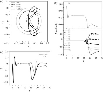
For large enough step changes in the far-field pressure the asymmetric shapes that emerge in the process of achieving static equilibrium are characterized by contact in the pole region as well; see also figure 14(a) obtained for the case with $\unicode[STIX]{x1D700}=3$ and $\unicode[STIX]{x1D712}=0.24~\text{N}~\text{m}^{-1}$ . This pattern of gradual increase of the asymmetry along this solution family, leading towards crescent-shaped shells and shells with contact at the pole region, was also observed in the static analysis of constant volume and constant pressure hard polymeric shells (Knoche & Kierfeld Reference Knoche and Kierfeld2011), with the exception that in the latter study the relevant asymmetric branch proceeded towards small compression levels as the external overpressure increased. Furthermore, in the latter study a static equilibrium with the opposite sides in contact is energetically favoured by hard shells when they are subjected to overpressures both above and below the buckling threshold. In the present study the strain-softening nature of phospholipid shells generates prohibitively large in-plane stresses at mildly large compression levels, and consequently a combination of bending and compression is enough for static equilibrium to be sustained; see also figure 12(a,b) exhibiting asymmetric shapes before contact regions are established.

As the external overpressure increases, shell viscosity reduces the compressive stresses in the pole region, prevents areas of intense bending or stretching from appearing in the pole region, and consequently jet formation is negated. The pattern captured in figure 11 for symmetric shapes was reproduced by the simulations for a larger initial overpressure (figure 14) when $\unicode[STIX]{x1D700}=3$ , that gradually lead to a static arrangement with asymmetric contact regions. In particular, the process of static buckling begins sooner as a result of the larger overpressure and the bubble continues to deform until it collapses with the two poles coalescing along the axis of symmetry. The poles of the bubble start to move inwards after a certain time with an increasing velocity, but soon enough the velocity starts decreasing due to the action of shell viscosity. The difference in the case of figure 14(a) lies in the evolution of curvatures in the regions around the two poles. The north pole, $\unicode[STIX]{x1D709}=0$ , exhibits a similar behaviour as in figure 11(a) with progressively smaller bending stresses as the interface retracts to a spherical shape. The south pole acquires an almost flat shape as it approaches static equilibrium, it takes longer to decelerate and coalesces with the north pole as it moves in the same direction but with a larger speed, before the microbubble settles down to a full static equilibrium. Nevertheless, there is no tendency for jet formation as the speed of the interface gradually vanishes, and the tendency for static equilibrium to be achieved is illustrated. Clearly, a significantly larger numerical effort is required in order to capture the point of contact with greater accuracy, and this was not pursued in the present study.

The above process, that leads to the establishment of shapes with contact, was a recurring theme in this study and is in marked contrast with the collapse process via jet formation that is typical for conventional bubbles. The latter type of bubbles exhibit jet formation even in the absence of a nearby wall (Dear & Field Reference Dear and Field1988), provided a large enough initial excitation is applied for fixed viscosity of the surrounding liquid. As was illustrated by the simulations performed in the present study, this is not the case with coated microbubbles, which exhibit a different type of finite time singularity during the ‘collapse’ process, that does not involve jet formation or formation of toroidal and satellite bubbles. Instead of pinching and the onset of areas of very large curvature at the points of contact, the regions of contact that are established around the two poles of coated microbubbles, provided the initial pressure disturbance is large enough, are characterized by finite curvature, small strain and significantly reduced speed under the combined action of shell viscosity and elasticity in the manner described in the above paragraphs. This process is conjectured to lead to the formation of almost flat contact regions in the vicinity of the two poles, such as often captured under static loading of shells.

Further increase of the area dilatation modulus $\unicode[STIX]{x1D712}$ to 0.96 further decreases the bending to stretching, $k_{b}/(\unicode[STIX]{x1D712}R_{0}^{2})\approx 0.0025,$ and volume compression to area dilatation, $P_{St}R_{0}/\unicode[STIX]{x1D712}\approx 0.375,$ stiffness ratios, thus favouring bending and volume compression in the post-buckling regime. Indeed, as illustrated in figure 15(a), obtained for an external overpressure with $\unicode[STIX]{x1D700}$ set to 1.3, the time evolution of the microbubble towards a static arrangement is dominated by $\text{P}_{4}$ (figure 15 b), and is symmetric with multiple bending regions and significant volume compression. This static shape corresponds to a different solution family than the prolate/oblate and asymmetric ones examined thus far, that also evolves to exhibit contact regions at larger external overpressures. In fact, upon increasing the external overpressure to 2, the pattern towards a static configuration with contact regions is recovered (figure 16 a), with the kinetic energy gradually dissipated in favour of bending and volume compression (figure 16 d). As a result of the prolonged action of shell viscosity (figure 16 e), growth of bending stresses is arrested in the region around the two poles and is restricted to the equator region. The former region acquires an almost spherical shape in the manner previously described for symmetric shapes in figure 11; see also the stress distribution along the shell provided in figure 16(f).

Figure 15.

(a) Temporal evolution of bubble shape and (b) temporal evolution of shape mode decomposition for a contrast agent ( $R=3.6~\unicode[STIX]{x03BC}\text{m}$ , $\unicode[STIX]{x1D707}_{s}=20~\text{Pa}~\text{s}$ , $\text{thickness}=1~\text{nm}$ , $\unicode[STIX]{x1D712}=0.96~\text{N}~\text{m}^{-1}$ , $k_{b}=3\times 10^{-14}~\text{N}~\text{m}$ ) for a step change disturbance with $\unicode[STIX]{x1D700}=1.3$ .

Figure 16.

(a) Temporal evolution of bubble shape ( $R=3.6~\unicode[STIX]{x03BC}\text{m}$ , $\unicode[STIX]{x1D707}_{s}=20~\text{Pa}~\text{s}$ , $\text{thickness}=1~\text{nm}$ , $\unicode[STIX]{x1D712}=0.96~\text{N}~\text{m}^{-1}$ , $k_{b}=3\times 10^{-14}~\text{N}~\text{m}$ ) for a step change disturbance ( $\unicode[STIX]{x1D700}=2$ ). (b) Time evolution of the radial velocity at the two poles. (c) Total shell energy, (d) distribution among different forms of energy and (e) shell damping as a function of time for $\unicode[STIX]{x1D700}=2$ . (f) Spatial distribution of shell and viscous stresses at $t=18.5$ .

In an attempt to explore how the viscous forces of the surrounding liquid affect the dynamic behaviour of the contrast agent and to investigate the extent to which they contribute in reaching the final static state we repeat the simulation presented in figure 12 with decreasing liquid viscosity: $\unicode[STIX]{x1D707}_{w}=10^{-4}~\text{Pa}~\text{s}$ and $\unicode[STIX]{x1D707}_{w}=10^{-5}~\text{Pa}~\text{s}$ . The results are presented in figure 17 for the latter case, obtained with the elliptic mesh generation method on a grid of $200\times 80$ elements. Clearly, the final shape (figure 17 a) is exactly the same as in the case with water shown in figure 12(a). The only difference is that in the latter situation there is a slight delay in shape mode appearance due to viscous dissipation, whereas as the liquid viscosity decreases the amplitude of shape mode oscillations becomes more intense (figure 17 b), until a static solution is achieved. In fact, when the viscosity of the liquid is decreased significantly, as is the case when $\unicode[STIX]{x1D707}_{w}=10^{-5}~\text{Pa}~\text{s}$ , the intermediate symmetric static state is not reached but the dynamic response leads directly to the asymmetric solution. Eventually, regardless of the fluid viscosity, the bubble obtains the same asymmetric static shape shown in figure 12(a).

Figure 17.

(a) Final static state and (b) temporal evolution of shape modes, for a step change disturbance with amplitude $\unicode[STIX]{x1D700}=2$ when the viscosity of the surrounding liquid is $\unicode[STIX]{x1D707}_{w}=10^{-5}~\text{Pa}~\text{s}$ ; $\unicode[STIX]{x1D712}=0.24~\text{N}~\text{m}^{-1}$ .

Finally, we examine the importance of shell viscosity in the dynamic behaviour of contrast agents in order to determine the extent to which it determines the onset of static equilibrium. To this end we consider the contrast agent whose response is simulated in figures 12 and 13 and assume negligible shell viscosity. Figure 18(a) presents the shape evolution obtained for a step change disturbance with amplitude $\unicode[STIX]{x1D700}=2$ by using the elliptic mesh generation technique. It can be immediately gleaned from the above figure and from the time variation of the shape mode decomposition (figure 18 b), that in this case the bubble performs considerably more volume pulsations compared to the case with finite shell viscosity (figure 12), before it settles to the same static equilibrium. In particular, the shape modes appear sooner and their oscillations are more intense. Furthermore, the dynamic response pattern does not go through the isotropically compressed spherical state which is eliminated in the absence of shell damping, while the microbubble eventually settles to the same static shape as before, albeit in an oscillatory fashion. The latter response is attributed to the combined effect of liquid viscosity and elasticity that act in a stabilizing manner by redistributing the kinetic energy at the pole region and the energy due to compression into elastic stretching, bending and surface energy (figure 18 c,d). Finally upon further increasing the external pressure by setting $\unicode[STIX]{x1D700}$ to 3, the process of formation of contact regions is significantly altered as the poles exhibit significantly larger speeds and larger curvature at the point of contact, thus corroborating the importance of shell viscosity in preventing jet formation.

Figure 18.

(a) Temporal evolution of bubble shape and (b) temporal evolution of radius and shape mode decomposition for a contrast agent ( $R=3.6~\unicode[STIX]{x03BC}\text{m}$ , $\unicode[STIX]{x1D707}_{s}=0$ , $\text{thickness}=1~\text{nm}$ , $\unicode[STIX]{x1D712}=0.24~\text{N}~\text{m}^{-1}$ , $k_{b}=3\times 10^{-14}~\text{N}~\text{m}$ ) for a step change disturbance ( $\unicode[STIX]{x1D700}=2$ ) with the elliptic mesh method. (c) Radial velocity and (d) distribution of the shell energy among its different forms.