

1 Introduction
Natural sources of water such as oceans, rivers or lakes often contain dissolved substances or temperature variations which create gradients in the fluid density. Microparticles such as marine snow, particular organic matter, inorganic dust as well as organisms living in such environments such as phytoplankton, protists and other swimmers interact with the density stratified layers in the course of their motion. One example of such interactions is the process of sedimentation which takes place due to gravity driven forces and is ubiquitously found in nature. It is an important means for the transport from the surface to the deep ocean and plays a crucial role in the nutrient transport between the oceanic layers (Kindler, Khalili & Stocker Reference Kindler, Khalili and Stocker2010; Guidi et al. Reference Guidi, Chaffron, Bittner, Eveillard, Larhlimi, Roux, Darzi, Audic, Berline and Brum2016; Ardekani, Doostmohammadi & Desai Reference Ardekani, Doostmohammadi and Desai2017). Settling of dense solid particles in stratified layers of atmosphere is another example where particles interact with naturally formed isopycnals. In this case, knowledge of the settling rates of these particles is crucial for understanding their impact on the environment (Kellogg Reference Kellogg1980). It is thus of physical significance to understand the interaction of solid particles with density stratified environments.
Most of the previous studies involving motion in stratified fluids have focused on spherical particles (Doostmohammadi & Ardekani Reference Doostmohammadi and Ardekani2015; Ardekani et al. Reference Ardekani, Doostmohammadi and Desai2017). Initial works in this field primarily focused on the increased drag experienced by the sphere due to the generation of internal gravity waves in the fluid at high Reynolds numbers (Warren Reference Warren1960; Mowbray & Rarity Reference Mowbray and Rarity1967; Lofquist & Purtell Reference Lofquist and Purtell1984). In the creeping flow limit, Chadwick & Zvirin (Reference Chadwick and Zvirin1974) theoretically studied the horizontal viscous flow past a sphere immersed in a linearly density stratified and non-diffusive fluid with weak stratification. They observed that buoyancy becomes important only at a distance of  $r\sim Ri^{-1/3}$ away from the sphere, where
 $Ri$ is the viscous Richardson number. They employed the method of matched asymptotic expansions to solve the problem. Later, Zvirin & Chadwick (Reference Zvirin and Chadwick1975) extended their analysis for a sphere translating in the vertical direction. In both the cases, a drag enhancement of the order of
 $Ri^{1/3}$ was predicted even for negligible Reynolds numbers. The experimental validation of drag enhancement at small Reynolds numbers was done by Yick et al. (Reference Yick, Torres, Peacock and Stocker2009). They argued that, when viscous forces dominate, the enhanced drag is induced by the buoyancy force exerted by a region of fluid which is dragged down by the settling sphere. Ardekani & Stocker (Reference Ardekani and Stocker2010) analysed the flow due to point force singularities placed in a stratified fluid. They demonstrated the existence of a fundamental stratification length scale which is governed by a competition between buoyancy, diffusion and viscosity and found that particles as small as
 $O(100~\unicode[STIX]{x03BC}\text{m}{-}1~\text{mm})$ can be influenced by stratification. Later, Candelier, Mehaddi & Vauquelin (Reference Candelier, Mehaddi and Vauquelin2014) calculated the unsteady drag experienced by a slowly descending sphere at low Péclet numbers (
 $Pe$). In contrast to the study by Chadwick & Zvirin (Reference Chadwick and Zvirin1974) for high Péclet numbers, they noted that, for small
 $Pe$, buoyancy forces become important at a distance of
 $r\sim (RiPe)^{-1/4}$ away from the sphere, where
 $(RiPe)^{1/4}$ is a small parameter in their study which scales with
 $a/l_{s}$ where
 $a$ is the particle length scale and
 $l_{s}$ is fundamental length scale for stratification (Ardekani & Stocker Reference Ardekani and Stocker2010). They employed a matching procedure based on series expansions of generalized functions and found their results to be in good agreement with the numerical results reported by Yick et al. (Reference Yick, Torres, Peacock and Stocker2009). More recently, Mehaddi, Candelier & Mehlig (Reference Mehaddi, Candelier and Mehlig2018) used the framework developed by Candelier et al. (Reference Candelier, Mehaddi and Vauquelin2014) to analyse the effect of convective fluid inertia on the drag experienced by a settling sphere in a density stratified fluid. We note that most of the above theoretical works use the standard method devised by Saffman (Reference Saffman1965) and Childress (Reference Childress1981) for analysing the inertial effect of a non-uniform background flow on the lift force experienced by the particle. The applicability of this method for arbitrarily shaped particles has been demonstrated in the literature, as is evident from the theoretical works employed to obtain leading-order inertial corrections for arbitrarily shaped particles moving in linear flow fields (Harper & Chang Reference Harper and Chang1968).
Particles settling in natural waters often have shapes which deviate from the spherical geometry, such as cylinders or disks (Turner & Holmes Reference Turner and Holmes2011). More generally, organic aggregates might have arbitrary body structures while settling in the fluid. Although a significant literature exists for spherical objects translating in stratified fluids, there is a dearth of studies concerning non-spherical particles. For a non-spherical particle, the orientation might change with time because of the torque exerted by the hydrodynamic forces. Analysis in this direction was started by Doostmohammadi & Ardekani (Reference Doostmohammadi and Ardekani2014), who numerically studied the motion of a spheroid oriented at an arbitrary angle and translating in a stratified fluid. They observed that, in addition to the extra drag experienced by the spheroid, stratification causes the long axis of the spheroid to orient parallel to the settling direction, in contrast to the counterpart in a homogeneous fluid. Hence, the stratification induced torque is non-zero and affects the settling dynamics of the spheroid. Experimental studies of settling of disks in a density stratified fluid have also reported a non-zero stratification induced torque acting on the disk (Mrokowska Reference Mrokowska2018; Mercier et al. Reference Mercier, Wang, Péméja, Ern and Ardekani2020).
Despite the ecological implications of settling particles in stratified environments, there are no theoretical studies concerning the drag force and change in orientation of a non-spherical particle settling in a stratified fluid. We thus understand that a more generalized study is required to shed light upon these problems. Sedimentation of particles in a homogeneous fluid has been studied extensively. It is known that at zero inertia, a non-skew particle settling in a homogeneous fluid does not change its orientation (Brenner Reference Brenner1964). However, when weak inertial effects are included, there exists a non-zero torque acting on the particle, which changes its orientation even if the external torque is zero (Cox Reference Cox1965). Hence, deviations from the homogeneous conditions, however small, might lead to changes in the settling dynamics of the particle. This motivates us further to broaden our understanding about the motion of particles in stratified fluids.
In this study, we consider the motion of an arbitrarily shaped particle moving through a weakly density stratified fluid with a continuous linear stratification and negligible inertia. We use the method of matched asymptotic expansions to solve the equations of motion. We provide a general expression for the force and the torque acting on the particle in the presence of stratification in terms of the Stokes resistance tensors of the particle. We then apply our results to some specific type of particles and highlight the impact of stratification on the motion of these particles.
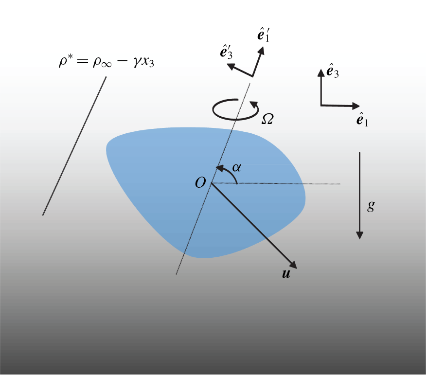
Rigid particle translating with a velocity  $\boldsymbol{u}$ and rotating with an angular velocity
 $\unicode[STIX]{x1D734}$. The ambient density is given by
 $\unicode[STIX]{x1D70C}^{\ast }=\unicode[STIX]{x1D70C}_{\infty }-\unicode[STIX]{x1D6FE}x_{3}$, where gravity
 $\boldsymbol{g}$ points in the negative
 $\hat{\boldsymbol{e}}_{3}$ direction. Here
 $(\hat{\boldsymbol{e}}_{1}-\hat{\boldsymbol{e}}_{2}-\hat{\boldsymbol{e}}_{3})$ is the laboratory coordinate system and
 $(\hat{\boldsymbol{e}}_{1}^{\prime }-\hat{\boldsymbol{e}}_{2}^{\prime }-\hat{\boldsymbol{e}}_{3}^{\prime })$ is the coordinate system fixed on the particle.

2 Problem formulation
Consider a rigid particle  $B$ of arbitrary shape having density
 $\unicode[STIX]{x1D70C}_{p}$, which is translating with a velocity
 $\boldsymbol{u}$ and rotating with an angular velocity
 $\unicode[STIX]{x1D734}$ in a linearly density stratified fluid (refer to figure 1). Here,
 $O$ is a point fixed in the particle and
 $(\hat{\boldsymbol{e}}_{1}^{\prime }-\hat{\boldsymbol{e}}_{2}^{\prime }-\hat{\boldsymbol{e}}_{3}^{\prime })$ denotes the system of coordinates fixed on the particle and passing through
 $O$. The ambient or the undisturbed density variations in the fluid are given by
 $$\begin{eqnarray}\unicode[STIX]{x1D70C}^{\ast }=\unicode[STIX]{x1D70C}_{\infty }-\unicode[STIX]{x1D6FE}x_{3}.\end{eqnarray}$$
Here,  $\unicode[STIX]{x1D70C}_{\infty }$ is the reference fluid density,
 $\unicode[STIX]{x1D6FE}$ is the density gradient in the vertical direction and
 $x_{3}$ is the third component of the coordinate vector
 $\boldsymbol{x}$ in the laboratory frame of reference.
2.1 Governing equations
We now write the equations of motion for the fluid in a frame of reference translating with point  $O$. We use the Boussinesq approximation and neglect the density variation in all the terms of the equations governing flow except the buoyancy force term (Candelier et al. Reference Candelier, Mehaddi and Vauquelin2014; Doostmohammadi, Dabiri & Ardekani Reference Doostmohammadi, Dabiri and Ardekani2014). The equations are given as follows:
 $$\begin{eqnarray}\displaystyle & \displaystyle \unicode[STIX]{x1D735}\boldsymbol{\cdot }\boldsymbol{w}=0, & \displaystyle\end{eqnarray}$$
 $$\begin{eqnarray}\displaystyle & \displaystyle \unicode[STIX]{x1D70C}_{\infty }\left({\displaystyle \frac{\unicode[STIX]{x2202}\boldsymbol{w}}{\unicode[STIX]{x2202}t}}+\boldsymbol{w}\boldsymbol{\cdot }\unicode[STIX]{x1D735}\boldsymbol{w}\right)=-\unicode[STIX]{x1D735}p+\unicode[STIX]{x1D70C}\boldsymbol{g}+\unicode[STIX]{x1D707}\unicode[STIX]{x1D6FB}^{2}\boldsymbol{w}-\unicode[STIX]{x1D70C}_{\infty }{\displaystyle \frac{\text{d}\boldsymbol{u}}{\text{d}t}}, & \displaystyle\end{eqnarray}$$
 $$\begin{eqnarray}\displaystyle & \displaystyle \boldsymbol{w}=\unicode[STIX]{x1D734}\times \boldsymbol{r}\quad \text{on }B,\quad \boldsymbol{w}\rightarrow -\boldsymbol{u}\quad \text{as }r=|\boldsymbol{r}|\rightarrow \infty . & \displaystyle\end{eqnarray}$$
Equations (2.2) and (2.3) represent the continuity equation and the momentum conservation equation in the fluid, respectively. Here,  $\boldsymbol{w}$ is the velocity of the fluid measured in the translating frame of reference.
When the changes in the concentration/temperature are linearly related to the changes in the density, we can solve for the advection–diffusion equation for the density (2.5), instead of such an equation for the temperature or concentration. The equation is given as follows:
 $$\begin{eqnarray}\displaystyle & \displaystyle {\displaystyle \frac{\unicode[STIX]{x2202}\unicode[STIX]{x1D70C}}{\unicode[STIX]{x2202}t}}+\boldsymbol{w}\boldsymbol{\cdot }\unicode[STIX]{x1D735}\unicode[STIX]{x1D70C}=\unicode[STIX]{x1D705}\unicode[STIX]{x1D6FB}^{2}\unicode[STIX]{x1D70C}, & \displaystyle\end{eqnarray}$$
 $$\begin{eqnarray}\displaystyle & \displaystyle \unicode[STIX]{x1D735}\unicode[STIX]{x1D70C}\boldsymbol{\cdot }\boldsymbol{n}=0\quad \text{on }B,\quad \unicode[STIX]{x1D70C}\rightarrow \unicode[STIX]{x1D70C}^{\ast }\quad \text{as }r\rightarrow \infty , & \displaystyle\end{eqnarray}$$
where  $\unicode[STIX]{x1D705}$ is the diffusivity coefficient and
 $\boldsymbol{n}$ represents the outward normal vector on the surface of the particle. Here, we have applied a no-flux boundary condition for the density field on the surface of the particle. If the stratification is induced due to gradients in concentration, this means that the surface of the particle is impermeable; whereas it implies an adiabatic boundary condition at the surface in the case of thermal gradients.
We non-dimensionalize the equations using the following scales: length scale  $l_{c}=l$, which denotes the characteristic geometric dimension of the particle, velocity scale
 $u_{c}=2/9l_{c}^{2}g/\unicode[STIX]{x1D708}(\unicode[STIX]{x1D70C}_{p}/\unicode[STIX]{x1D70C}_{\infty }-1)$, which denotes the terminal Stokes velocity evaluated for a sphere of radius
 $l_{c}$, and density
 $\unicode[STIX]{x1D70C}_{p}$ settling in a homogeneous fluid with ambient density
 $\unicode[STIX]{x1D70C}_{\infty }$, time scale
 $t_{c}=\unicode[STIX]{x1D70F}$, pressure scale
 $p_{c}=\unicode[STIX]{x1D707}(u_{c}/l)$, density scale
 $\unicode[STIX]{x1D70C}_{c}=\unicode[STIX]{x1D6FE}l$. Here,
 $\unicode[STIX]{x1D70F}$ is the time scale of variations of the disturbance velocity. We use the same variables to denote the dimensionless variables. The dimensionless governing equations are thus written as follows:
 $$\begin{eqnarray}\displaystyle & \displaystyle \unicode[STIX]{x1D735}\boldsymbol{\cdot }\boldsymbol{w}=0, & \displaystyle\end{eqnarray}$$
 $$\begin{eqnarray}\displaystyle & \displaystyle ReSl{\displaystyle \frac{\unicode[STIX]{x2202}\boldsymbol{w}}{\unicode[STIX]{x2202}t}}+Re\left(\boldsymbol{w}\boldsymbol{\cdot }\unicode[STIX]{x1D735}\boldsymbol{w}\right)=-\unicode[STIX]{x1D735}p-Ri\unicode[STIX]{x1D70C}\hat{\boldsymbol{e}}_{3}+\unicode[STIX]{x1D6FB}^{2}\boldsymbol{w}-ReSl{\displaystyle \frac{\text{d}\boldsymbol{u}}{\text{d}t}}, & \displaystyle\end{eqnarray}$$
 $$\begin{eqnarray}\displaystyle & \displaystyle PeSl{\displaystyle \frac{\unicode[STIX]{x2202}\unicode[STIX]{x1D70C}}{\unicode[STIX]{x2202}t}}+Pe\left(\boldsymbol{w}\boldsymbol{\cdot }\unicode[STIX]{x1D735}\unicode[STIX]{x1D70C}\right)=\unicode[STIX]{x1D6FB}^{2}\unicode[STIX]{x1D70C}. & \displaystyle\end{eqnarray}$$
Here,  $Re=(\unicode[STIX]{x1D70C}_{\infty }u_{c}l)/\unicode[STIX]{x1D707}$ is the Reynolds number,
 $Pe=u_{c}l/\unicode[STIX]{x1D705}$ is the Péclet number,
 $Ri=\unicode[STIX]{x1D6FE}gl^{3}/\unicode[STIX]{x1D707}u_{c}$ is the viscous Richardson number which is the product of the Richardson number, used in the stratified flow literature, denoting the ratio of buoyancy and inertial forces and the Reynolds number. We use the viscous Richardson number because
 $Ri^{-1/3}$ represents the distance at which the buoyancy forces balance the viscous forces at large
 $Pe$ and it appears in our solution. The parameter
 $Sl=l/u_{c}\unicode[STIX]{x1D70F}$ is the Strouhal number.
We now express the velocity, pressure and the density in terms of disturbed and undisturbed variables,  $\boldsymbol{w}=\boldsymbol{w}^{\prime }-\boldsymbol{u}$,
 $\unicode[STIX]{x1D70C}=\unicode[STIX]{x1D70C}^{\ast }+\unicode[STIX]{x1D70C}^{\prime },$ and
 $p=p^{\ast }+p^{\prime }$. We note that the undisturbed pressure balances the undisturbed density field. Additionally, we note that
 $\unicode[STIX]{x2202}\unicode[STIX]{x1D70C}^{\ast }/\unicode[STIX]{x2202}t=-\boldsymbol{u}\boldsymbol{\cdot }\hat{\boldsymbol{e}}_{3}/Sl$ and
 $\unicode[STIX]{x1D735}\unicode[STIX]{x1D70C}^{\ast }=-\hat{\boldsymbol{e}}_{3}$. As a result, we obtain
 $$\begin{eqnarray}\displaystyle & \displaystyle \unicode[STIX]{x1D735}\boldsymbol{\cdot }\boldsymbol{w}^{\prime }=0, & \displaystyle\end{eqnarray}$$
 $$\begin{eqnarray}\displaystyle & \displaystyle ReSl{\displaystyle \frac{\unicode[STIX]{x2202}\boldsymbol{w}^{\prime }}{\unicode[STIX]{x2202}t}}+Re\left((\boldsymbol{w}^{\prime }-\boldsymbol{u})\boldsymbol{\cdot }\unicode[STIX]{x1D735}\boldsymbol{w}^{\prime }\right)=-\unicode[STIX]{x1D735}p^{\prime }-Ri\unicode[STIX]{x1D70C}^{\prime }\hat{\boldsymbol{e}}_{3}+\unicode[STIX]{x1D6FB}^{2}\boldsymbol{w}^{\prime }, & \displaystyle\end{eqnarray}$$
 $$\begin{eqnarray}\displaystyle & \displaystyle PeSl{\displaystyle \frac{\unicode[STIX]{x2202}\unicode[STIX]{x1D70C}^{\prime }}{\unicode[STIX]{x2202}t}}-Pe(\boldsymbol{w}^{\prime }\boldsymbol{\cdot }\hat{\boldsymbol{e}}_{3})+Pe\left((\boldsymbol{w}^{\prime }-\boldsymbol{u})\boldsymbol{\cdot }\unicode[STIX]{x1D735}\unicode[STIX]{x1D70C}^{\prime }\right)=\unicode[STIX]{x1D6FB}^{2}\unicode[STIX]{x1D70C}^{\prime }. & \displaystyle\end{eqnarray}$$
 $$\begin{eqnarray}\displaystyle & \displaystyle \boldsymbol{w}^{\prime }=\boldsymbol{u}+\unicode[STIX]{x1D734}\times \boldsymbol{r}\quad \text{on }B,\quad \boldsymbol{w}^{\prime }\rightarrow \mathbf{0}\quad \text{as }r\rightarrow \infty , & \displaystyle \nonumber\\ \displaystyle & \displaystyle \unicode[STIX]{x1D735}\unicode[STIX]{x1D70C}^{\prime }\boldsymbol{\cdot }\boldsymbol{n}=-\unicode[STIX]{x1D735}\unicode[STIX]{x1D70C}^{\ast }\boldsymbol{\cdot }\boldsymbol{n}\quad \text{on }B,\quad \unicode[STIX]{x1D70C}^{\prime }\rightarrow 0\quad \text{as }r\rightarrow \infty . & \displaystyle \nonumber\end{eqnarray}$$
We will solve equations (2.10)–(2.12) by making the following assumptions. Firstly, we assume that the velocity of the particle is small enough such that the inertial effects are negligible. Next, we assume that the stratification effects are small but non-negligible. As a result, we will analyse the problem in the following limits:
 $$\begin{eqnarray}Re\ll \min (Ri^{1/3},(RiPe)^{1/4}),\quad Ri\ll 1.\end{eqnarray}$$
For a density stratified fluid, as the particle descends, it encounters a variable fluid density. Thus, the problem appears to be unsteady as the buoyancy force experienced by the particle is changing with time. However, if the stratification is weak, then we expect the time scale of variation for the particle velocity to be long enough such that the motion of the particle can be assumed to be quasi-steady. Similar to the quasi-steady state analysis performed by Mehaddi et al. (Reference Mehaddi, Candelier and Mehlig2018), we expect the time scale of variation ( $\unicode[STIX]{x1D70F}$) to scale as
 $\unicode[STIX]{x1D70F}\sim u_{t}/u_{t}^{\prime }$, where
 $u_{t}=2/9(l^{2}g/\unicode[STIX]{x1D708})(\unicode[STIX]{x1D70C}_{p}/\unicode[STIX]{x1D70C}^{\ast }-1)$ denotes the terminal Stokes velocity evaluated for a sphere settling in a fluid with the ambient density
 $\unicode[STIX]{x1D70C}^{\ast }$, which depends on the particle position and
 $u_{t}^{\prime }$ denotes the time derivative of
 $u_{t}$. We substitute this scaling in the expression for
 $Sl$ and obtain the following:
 $$\begin{eqnarray}Sl\sim Ri{\displaystyle \frac{\unicode[STIX]{x1D70C}_{p}}{\unicode[STIX]{x1D70C}_{\infty }}}.\end{eqnarray}$$
Hence, if  $Ri\ll 1$, the time scale of variation of the particle velocity is long enough such that the condition
 $Sl\ll 1$ is also satisfied. Thus, the unsteady terms and the convective inertial terms in (2.11) and (2.12) can be neglected.
We note that the Péclet number  $Pe$ =
 $RePr$, where the Prandtl number (
 $Pr$) is the ratio between the momentum diffusivity and the diffusivity of the stratifying agent in the fluid. For the sake of brevity, we use the notations of Péclet and Prandtl numbers for the case of stratification caused by salt transport as well, even though these numbers are called the Sherwood and Schmidt numbers in the literature. For the limit of negligible
 $Re$ considered in our problem, a high Péclet number (
 $Pe\gg 1$) corresponds to a large Prandtl number (
 $Pr\gg 1$), as is the case for salt stratified water (
 $Pr=700$) or temperature stratified viscous oils or greases (
 $Pr\sim 10^{3}-10^{6}$) (Leal Reference Leal2007). A low Péclet number (
 $Pe\ll 1$) corresponds to a Prandtl number of
 $O(1)$ or even less, as is the case for temperature stratified air at room temperature (
 $Pr=0.71$) or molten metals (
 $Pr\sim 0.001-0.01$).
3 Solution
For a sphere settling in a linearly stratified fluid, it is known that Stokes solution is not a uniformly valid first approximation to the flow for small stratification strengths (Mehaddi et al. Reference Mehaddi, Candelier and Mehlig2018). At sufficiently large distances from the particle, the buoyancy forces will become important and have to be taken into account. This is an indicator of a singular asymptotic behaviour and a regular perturbation expansion of the field variables in terms of  $Ri$ is not valid. As the scaling analysis involved in these findings is independent of the shape of the particle, we expect similar behaviour even if the particle shape is arbitrary. For large Péclet numbers, Zvirin & Chadwick (Reference Zvirin and Chadwick1975) estimated the matching zone to occur at a distance of
 $r\sim Ri^{-1/3}$ away from the particle. Hence, the appropriate length scale far away from the particle is
 $l_{c}=lRi^{-1/3}$. Even though this scaling is valid only for high Péclet numbers (
 $Pe>Ri^{1/3}$), Zvirin & Chadwick (Reference Zvirin and Chadwick1975) did not make any assumptions regarding the Péclet number while solving the equations of motion in the outer zone (
 $r>Ri^{-1/3}$), and reported the drag coefficients for any arbitrary
 $Pe$. Later, Mehaddi et al. (Reference Mehaddi, Candelier and Mehlig2018) developed a methodology which is uniformly valid for any Prandtl number (
 $Pr$) by considering spherical particles, which confirmed the results reported by Zvirin & Chadwick (Reference Zvirin and Chadwick1975) and hence established that their results are more generally valid for any
 $Pr$. This can be rationalized by considering that the stratification induced force and torque acting on the particle depend only on the leading-order outer solution, which was solved for arbitrary Péclet number by Zvirin & Chadwick (Reference Zvirin and Chadwick1975). If the outer solution is expressed in terms of the leading-order drag experienced by the particle, it does not depend on the shape of the particle. Hence, adopting the procedure reported by Zvirin & Chadwick (Reference Zvirin and Chadwick1975), we can calculate the stratification induced hydrodynamic force and torque on an arbitrarily shaped particle for any
 $Pr$ even though the scales used in such a calculation are physically relevant only at large Péclet numbers. We seek to solve the problem by using the method of matched asymptotic expansions using the small parameter
 $\unicode[STIX]{x1D716}=Ri^{1/3}$. We shall start by writing the inner and the outer equations.
3.1 Inner equations
The inner equations are given as follows:
 $$\begin{eqnarray}\displaystyle & \displaystyle -\unicode[STIX]{x1D735}p^{\prime }+\unicode[STIX]{x1D6FB}^{2}\boldsymbol{w}^{\prime }=\unicode[STIX]{x1D716}^{3}\unicode[STIX]{x1D70C}^{\prime }\hat{\boldsymbol{e}}_{3}+Re\left((\boldsymbol{w}^{\prime }-\boldsymbol{u})\boldsymbol{\cdot }\unicode[STIX]{x1D735}\boldsymbol{w}^{\prime }\right),\quad \unicode[STIX]{x1D735}\boldsymbol{\cdot }\boldsymbol{w}^{\prime }=0, & \displaystyle\end{eqnarray}$$
 $$\begin{eqnarray}\displaystyle & \displaystyle -Pe(\boldsymbol{w}^{\prime }\boldsymbol{\cdot }\hat{\boldsymbol{e}}_{3})+Pe((\boldsymbol{w}^{\prime }-\boldsymbol{u})\boldsymbol{\cdot }\unicode[STIX]{x1D735}\unicode[STIX]{x1D70C}^{\prime })=\unicode[STIX]{x1D6FB}^{2}\unicode[STIX]{x1D70C}^{\prime }, & \displaystyle\end{eqnarray}$$
 $$\begin{eqnarray}\displaystyle & \displaystyle \boldsymbol{w}^{\prime }=\boldsymbol{u}+\unicode[STIX]{x1D734}\times \boldsymbol{r},\quad \unicode[STIX]{x1D735}\unicode[STIX]{x1D70C}^{\prime }\boldsymbol{\cdot }\boldsymbol{n}=-\unicode[STIX]{x1D735}\unicode[STIX]{x1D70C}^{\ast }\boldsymbol{\cdot }\boldsymbol{n}\quad \text{on }B. & \displaystyle\end{eqnarray}$$
 $$\begin{eqnarray}\{\boldsymbol{w}^{\prime },p^{\prime },\unicode[STIX]{x1D70C}^{\prime }\}=\{\boldsymbol{w}_{0},p_{0},\unicode[STIX]{x1D70C}_{0}\}+\unicode[STIX]{x1D716}\{\boldsymbol{w}_{1},p_{1},\unicode[STIX]{x1D70C}_{1}\}+o(\unicode[STIX]{x1D716}).\end{eqnarray}$$
The gauge functions in this expansion ( $1,\unicode[STIX]{x1D716},\ldots$) can be rigorously derived for a spherical particle (Chadwick & Zvirin Reference Chadwick and Zvirin1974; Zvirin & Chadwick Reference Zvirin and Chadwick1975) and we expect the same gauge functions to occur for any arbitrarily shaped particle. We substitute these expressions in (3.1) and collect the terms at various orders of
 $\unicode[STIX]{x1D716}$ to obtain the following. At
 $O(1)$,
 $$\begin{eqnarray}\displaystyle & \displaystyle -\unicode[STIX]{x1D735}p_{0}+\unicode[STIX]{x1D6FB}^{2}\boldsymbol{w}_{0}=\mathbf{0},\quad \unicode[STIX]{x1D735}\boldsymbol{\cdot }\boldsymbol{w}_{0}=0, & \displaystyle\end{eqnarray}$$
 $$\begin{eqnarray}\displaystyle & \displaystyle -Pe(\boldsymbol{w}_{0}\boldsymbol{\cdot }\hat{\boldsymbol{e}}_{3})+Pe\left((\boldsymbol{w}_{0}-\boldsymbol{u})\boldsymbol{\cdot }\unicode[STIX]{x1D735}\unicode[STIX]{x1D70C}_{0}\right)=\unicode[STIX]{x1D6FB}^{2}\unicode[STIX]{x1D70C}_{0}, & \displaystyle\end{eqnarray}$$
 $$\begin{eqnarray}\displaystyle & \displaystyle \boldsymbol{w}_{0}=\boldsymbol{u}+\unicode[STIX]{x1D734}\times \boldsymbol{r},\quad \unicode[STIX]{x1D735}\unicode[STIX]{x1D70C}_{0}\boldsymbol{\cdot }\boldsymbol{n}=-\unicode[STIX]{x1D735}\unicode[STIX]{x1D70C}^{\ast }\boldsymbol{\cdot }\boldsymbol{n}\quad \text{on }B. & \displaystyle\end{eqnarray}$$
 $O(\unicode[STIX]{x1D716})$,
 $$\begin{eqnarray}\displaystyle & \displaystyle -\unicode[STIX]{x1D735}p_{1}+\unicode[STIX]{x1D6FB}^{2}\boldsymbol{w}_{1}=\mathbf{0},\quad \unicode[STIX]{x1D735}\boldsymbol{\cdot }\boldsymbol{w}_{1}=0, & \displaystyle\end{eqnarray}$$
 $$\begin{eqnarray}\displaystyle & \displaystyle -Pe(\boldsymbol{w}_{1}\boldsymbol{\cdot }\hat{\boldsymbol{e}}_{3})+Pe\left((\boldsymbol{w}_{0}-\boldsymbol{u})\boldsymbol{\cdot }\unicode[STIX]{x1D735}\unicode[STIX]{x1D70C}_{1}+\boldsymbol{w}_{1}\boldsymbol{\cdot }\unicode[STIX]{x1D735}\unicode[STIX]{x1D70C}_{0}\right)=\unicode[STIX]{x1D6FB}^{2}\unicode[STIX]{x1D70C}_{1}, & \displaystyle\end{eqnarray}$$
 $$\begin{eqnarray}\displaystyle & \displaystyle \boldsymbol{w}_{1}=\mathbf{0},\quad \unicode[STIX]{x1D735}\unicode[STIX]{x1D70C}_{1}\boldsymbol{\cdot }\boldsymbol{n}=0\quad \text{on }B. & \displaystyle\end{eqnarray}$$
3.2 Outer equations
For the outer expansion, we rescale the coordinate system such that all terms are of equal orders of magnitude. We thus use the following transformation:
 $$\begin{eqnarray}\tilde{\boldsymbol{r}}=\unicode[STIX]{x1D716}\boldsymbol{r},\quad \tilde{\unicode[STIX]{x1D735}}={\displaystyle \frac{\unicode[STIX]{x1D735}}{\unicode[STIX]{x1D716}}}.\end{eqnarray}$$
Based on the method used by Childress (Reference Childress1964) and Saffman (Reference Saffman1965), in the far field region, the rigid particle can be replaced by a point force, with a strength equal to the negative of the Stokes drag. We express the non-dimensional Stokes drag acting on the particle as  $\boldsymbol{F}_{0}$. As the far field representation of the leading-order disturbance flow is a Stokeslet, we expect that, for
 $r\gg 1$, the flow
 $\boldsymbol{w}^{\prime }\sim 1/r\ll \boldsymbol{u}$. Consequently, we have
 $\boldsymbol{w}^{\prime }\boldsymbol{\cdot }\unicode[STIX]{x1D735}\unicode[STIX]{x1D70C}^{\prime }\ll \boldsymbol{u}\boldsymbol{\cdot }\unicode[STIX]{x1D735}\unicode[STIX]{x1D70C}^{\prime }$ and thus
 $\boldsymbol{w}^{\prime }\boldsymbol{\cdot }\unicode[STIX]{x1D735}\unicode[STIX]{x1D70C}^{\prime }$ can be neglected in the outer equations. We also rescale the velocity and pressure fields by writing
 $\boldsymbol{w}^{\prime }=\unicode[STIX]{x1D716}\tilde{\boldsymbol{w}}$ and
 $p^{\prime }=\unicode[STIX]{x1D716}^{2}\tilde{p}$. Here, it should be noted that we have made no assumptions regarding the Péclet number in the outer equations, which are written for any arbitrary value of
 $Pe$. We can now write the outer equations as follows:
 $$\begin{eqnarray}\displaystyle & \displaystyle \tilde{\unicode[STIX]{x1D735}}\boldsymbol{\cdot }\tilde{\boldsymbol{w}}=0, & \displaystyle\end{eqnarray}$$
 $$\begin{eqnarray}\displaystyle & \displaystyle -\tilde{\unicode[STIX]{x1D735}}\tilde{p}+\tilde{\unicode[STIX]{x1D735}}^{2}\tilde{\boldsymbol{w}}=\unicode[STIX]{x1D70C}^{\prime }\hat{\boldsymbol{e}}_{3}+\boldsymbol{F}_{0}\unicode[STIX]{x1D6FF}(\tilde{\boldsymbol{r}}), & \displaystyle\end{eqnarray}$$
 $$\begin{eqnarray}\displaystyle & \displaystyle -\unicode[STIX]{x1D716}\tilde{\boldsymbol{w}}\boldsymbol{\cdot }\hat{\boldsymbol{e}}_{3}-\unicode[STIX]{x1D716}\boldsymbol{u}\boldsymbol{\cdot }\tilde{\unicode[STIX]{x1D735}}\unicode[STIX]{x1D70C}^{\prime }={\displaystyle \frac{\unicode[STIX]{x1D716}^{2}}{Pe}}\tilde{\unicode[STIX]{x1D735}}^{2}\unicode[STIX]{x1D70C}^{\prime }. & \displaystyle\end{eqnarray}$$
 $\tilde{\boldsymbol{w}},\tilde{p},\unicode[STIX]{x1D70C}^{\prime }$ as follows:
 $$\begin{eqnarray}\hat{\boldsymbol{w}}=\displaystyle \int \tilde{\boldsymbol{w}}\text{e}^{-\text{i}\boldsymbol{k}\boldsymbol{\cdot }\tilde{\boldsymbol{r}}}\,\text{d}\tilde{\boldsymbol{r}},\quad \hat{p}=\displaystyle \int \tilde{p}\text{e}^{-\text{i}\boldsymbol{k}\boldsymbol{\cdot }\tilde{\boldsymbol{r}}}\,\text{d}\tilde{\boldsymbol{r}},\quad \hat{\unicode[STIX]{x1D70C}}=\displaystyle \int \unicode[STIX]{x1D70C}^{\prime }\text{e}^{-\text{i}\boldsymbol{k}\boldsymbol{\cdot }\tilde{\boldsymbol{r}}}\,\text{d}\tilde{\boldsymbol{r}}.\end{eqnarray}$$
Here,  $\boldsymbol{k}=(k_{1},k_{2},k_{3})$ and
 $\boldsymbol{k}\boldsymbol{\cdot }\boldsymbol{k}=k^{2}.$ We can write the inverse Fourier transforms as follows:
 $$\begin{eqnarray}\tilde{\boldsymbol{w}}={\displaystyle \frac{\displaystyle \displaystyle \int \hat{\boldsymbol{w}}\text{e}^{\text{i}\boldsymbol{k}\boldsymbol{\cdot }\tilde{\boldsymbol{r}}}\,\text{d}\boldsymbol{k}}{8\unicode[STIX]{x03C0}^{3}}},\quad \tilde{p}={\displaystyle \frac{\displaystyle \displaystyle \int \hat{p}\text{e}^{\text{i}\boldsymbol{k}\boldsymbol{\cdot }\tilde{\boldsymbol{r}}}\,\text{d}\boldsymbol{k}}{8\unicode[STIX]{x03C0}^{3}}},\quad \unicode[STIX]{x1D70C}^{\prime }={\displaystyle \frac{\displaystyle \displaystyle \int \hat{\unicode[STIX]{x1D70C}}\text{e}^{\text{i}\boldsymbol{k}\boldsymbol{\cdot }\tilde{\boldsymbol{r}}}\,\text{d}\boldsymbol{k}}{8\unicode[STIX]{x03C0}^{3}}}.\end{eqnarray}$$
We substitute these expressions in (3.4) to obtain a set of linear equations in  $\hat{\boldsymbol{w}},\hat{p},\hat{\unicode[STIX]{x1D70C}}$ as follows:
 $$\begin{eqnarray}\displaystyle & \displaystyle \boldsymbol{k}\boldsymbol{\cdot }\hat{\boldsymbol{w}}=0, & \displaystyle\end{eqnarray}$$
 $$\begin{eqnarray}\displaystyle & \displaystyle \mathbf{0}=-\text{i}\boldsymbol{k}\hat{p}-k^{2}\hat{\boldsymbol{w}}-\hat{\unicode[STIX]{x1D70C}}\hat{\boldsymbol{e}}_{3}-\boldsymbol{F}_{0}, & \displaystyle\end{eqnarray}$$
 $$\begin{eqnarray}\displaystyle & \displaystyle \hat{\boldsymbol{w}}\boldsymbol{\cdot }\hat{\boldsymbol{e}}_{3}+\boldsymbol{u}\boldsymbol{\cdot }i\boldsymbol{k}\hat{\unicode[STIX]{x1D70C}}={\displaystyle \frac{\unicode[STIX]{x1D716}}{Pe}}k^{2}\hat{\unicode[STIX]{x1D70C}}. & \displaystyle\end{eqnarray}$$
 $\hat{\boldsymbol{w}}$ as follows:
 $$\begin{eqnarray}\hat{\boldsymbol{w}}=-\left(k^{2}\unicode[STIX]{x1D644}+{\displaystyle \frac{\hat{\boldsymbol{e}}_{3}\hat{\boldsymbol{e}}_{3}}{X}}-{\displaystyle \frac{\boldsymbol{k}\hat{\boldsymbol{e}}_{3}(\boldsymbol{k}\boldsymbol{\cdot }\hat{\boldsymbol{e}}_{3})}{Xk^{2}}}\right)^{-1}\left(\unicode[STIX]{x1D644}-{\displaystyle \frac{\boldsymbol{k}\boldsymbol{k}}{k^{2}}}\right)\boldsymbol{\cdot }\boldsymbol{F}_{0}.\end{eqnarray}$$
Here,  $X=\unicode[STIX]{x1D716}k^{2}/Pe-\text{i}\boldsymbol{u}\boldsymbol{\cdot }\boldsymbol{k}$.
We know that a part of the outer solution must match the leading-order inner solution far away from the particle, which corresponds to a Stokeslet. Hence, we now consider a flow field which corresponds to a Stokeslet which satisfies the Stokes equations with a point force  $\boldsymbol{F}_{0}$ acting at the origin. We again make use of the rescaled variable to obtain the following equations of motion:
 $$\begin{eqnarray}\displaystyle & \displaystyle \tilde{\unicode[STIX]{x1D735}}\boldsymbol{\cdot }\boldsymbol{w}_{s}=0. & \displaystyle\end{eqnarray}$$
 $$\begin{eqnarray}\displaystyle & \displaystyle \mathbf{0}=-\tilde{\unicode[STIX]{x1D735}}p_{s}+\unicode[STIX]{x1D716}\tilde{\unicode[STIX]{x1D735}}^{2}\boldsymbol{w}_{s}-\unicode[STIX]{x1D716}^{2}\boldsymbol{F}_{0}\unicode[STIX]{x1D6FF}(\tilde{\boldsymbol{r}}). & \displaystyle\end{eqnarray}$$
 $$\begin{eqnarray}\hat{\boldsymbol{w}}_{s}=\displaystyle \int \boldsymbol{w}_{s}\text{e}^{-\text{i}\boldsymbol{k}\boldsymbol{\cdot }\tilde{\boldsymbol{r}}}\,\text{d}\tilde{\boldsymbol{r}},\quad \hat{p}_{s}=\displaystyle \int p_{s}\text{e}^{-\text{i}\boldsymbol{k}\boldsymbol{\cdot }\tilde{\boldsymbol{r}}}\,\text{d}\tilde{\boldsymbol{r}}.\end{eqnarray}$$
We solve equations (3.7) in the Fourier space and obtain the solution for the Stokeslet as follows:
 $$\begin{eqnarray}\hat{\boldsymbol{w}}_{s}=-{\displaystyle \frac{\unicode[STIX]{x1D716}}{k^{2}}}\left(\unicode[STIX]{x1D644}-{\displaystyle \frac{\boldsymbol{k}\boldsymbol{k}}{k^{2}}}\right)\boldsymbol{\cdot }\boldsymbol{F}_{0}.\end{eqnarray}$$
Based on the methodology of the matched asymptotic expansions, we know that the inner and outer expansions should match in the matching zone. We thus have
 $$\begin{eqnarray}\lim _{r\rightarrow \infty }\boldsymbol{w}_{0}+\unicode[STIX]{x1D716}\boldsymbol{w}_{1}=\lim _{\tilde{r}\rightarrow 0}\boldsymbol{w}^{\prime }.\end{eqnarray}$$
Far away from the particle,  $\boldsymbol{w}_{0}$ asymptotes to a Stokeslet. As a result, we can write
 $$\begin{eqnarray}\lim _{r\rightarrow \infty }\boldsymbol{w}_{0}\sim \boldsymbol{w}_{s}.\end{eqnarray}$$
We now, express  $\boldsymbol{w}^{\prime },\boldsymbol{w}_{s}$ in terms of their inverse Fourier transforms and substitute in (3.9) to obtain
 $$\begin{eqnarray}\lim _{r\rightarrow \infty }\unicode[STIX]{x1D716}\boldsymbol{w}_{1}=\lim _{\tilde{r}\rightarrow 0}\displaystyle \int {\displaystyle \frac{(\unicode[STIX]{x1D716}\hat{\boldsymbol{w}}-\hat{\boldsymbol{w}}_{s})\text{e}^{\text{i}\boldsymbol{k}\boldsymbol{\cdot }\tilde{\boldsymbol{r}}}\,\text{d}\boldsymbol{k}}{8\unicode[STIX]{x03C0}^{3}}}.\end{eqnarray}$$
To evaluate the right side of the above equation, we shall adopt a similar approach to that used by Childress (Reference Childress1964) and Zvirin & Chadwick (Reference Zvirin and Chadwick1975) and divide the region of integration into two parts,  $0\leqslant k\leqslant \tilde{r}^{-\unicode[STIX]{x1D70E}},(0<\unicode[STIX]{x1D70E}<1)$ where the exponential is reduced to
 $1$ and
 $k>\tilde{r}^{-\unicode[STIX]{x1D70E}}$ for large values of
 $k$. Thus, the above equation can be decomposed into two parts as follows:
 $$\begin{eqnarray}\lim _{r\rightarrow \infty }\unicode[STIX]{x1D716}\boldsymbol{w}_{1}=\displaystyle \int {\displaystyle \frac{(\unicode[STIX]{x1D716}\hat{\boldsymbol{w}}-\hat{\boldsymbol{w}}_{s})\,\text{d}\boldsymbol{k}}{8\unicode[STIX]{x03C0}^{3}}}+\lim _{\tilde{r}\rightarrow 0}\displaystyle \int _{k>\tilde{r}^{-\unicode[STIX]{x1D70E}}}{\displaystyle \frac{(\unicode[STIX]{x1D716}\hat{\boldsymbol{w}}-\hat{\boldsymbol{w}}_{s})\text{e}^{\text{i}\boldsymbol{k}\boldsymbol{\cdot }\tilde{\boldsymbol{r}}}\,\text{d}\boldsymbol{k}}{8\unicode[STIX]{x03C0}^{3}}}.\end{eqnarray}$$
We also note that  $\boldsymbol{w}_{1}$ satisfies the Stokes equation (refer to (3.3a)). Hence, we can express
 $\boldsymbol{w}_{1}$ in the form of the Lamb’s general solution for creeping flow as follows:
 $$\begin{eqnarray}\boldsymbol{w}_{1}=\mathop{\sum }_{n=-\infty }^{\infty }\left(\unicode[STIX]{x1D735}\times (\boldsymbol{r}\unicode[STIX]{x1D712}_{n})+\unicode[STIX]{x1D735}\unicode[STIX]{x1D713}_{n}+{\displaystyle \frac{(n+3)}{2(n+1)(2n+3)}}r^{2}\unicode[STIX]{x1D735}p_{n}-{\displaystyle \frac{n}{(n+1)(2n+3)}}\boldsymbol{r}p_{n}\right).\end{eqnarray}$$
Here,  $\unicode[STIX]{x1D712}_{n},\unicode[STIX]{x1D713}_{n}$ and
 $p_{n}$ are solid spherical harmonics of order
 $n$. Hence, we can express the above velocity field in terms of powers of
 $r$ as follows:
 $$\begin{eqnarray}\boldsymbol{w}_{1}=\mathop{\sum }_{n=-\infty }^{\infty }A_{n}r^{n}\boldsymbol{f}_{n}(\unicode[STIX]{x1D703},\unicode[STIX]{x1D719}).\end{eqnarray}$$
Here,  $(r,\unicode[STIX]{x1D703},\unicode[STIX]{x1D719})$ represent the spherical coordinates with origin at
 $O$,
 $\boldsymbol{f}_{n}(\unicode[STIX]{x1D703},\unicode[STIX]{x1D719})$ are arbitrary vector functions of
 $\unicode[STIX]{x1D703},\unicode[STIX]{x1D719}$ and
 $A_{n}$ are constant coefficients. We now replace
 $r$ by
 $\tilde{r}/\unicode[STIX]{x1D716}$ to express
 $\boldsymbol{w}_{1}$ in terms of the outer variables and substitute in (3.11) to obtain the following expression:
 $$\begin{eqnarray}\mathop{\sum }_{n=-\infty }^{\infty }A_{n}\unicode[STIX]{x1D716}^{1-n}\tilde{r}^{n}\boldsymbol{f}_{n}(\unicode[STIX]{x1D703},\unicode[STIX]{x1D719})=\displaystyle \int {\displaystyle \frac{(\unicode[STIX]{x1D716}\hat{\boldsymbol{w}}-\hat{\boldsymbol{w}}_{s})\,\text{d}\boldsymbol{k}}{8\unicode[STIX]{x03C0}^{3}}}+\lim _{\tilde{r}\rightarrow 0}\displaystyle \int _{k>\tilde{r}^{-\unicode[STIX]{x1D70E}}}{\displaystyle \frac{(\unicode[STIX]{x1D716}\hat{\boldsymbol{w}}-\hat{\boldsymbol{w}}_{s})\text{e}^{\text{i}\boldsymbol{k}\boldsymbol{\cdot }\tilde{\boldsymbol{r}}}\,\text{d}\boldsymbol{k}}{8\unicode[STIX]{x03C0}^{3}}}.\end{eqnarray}$$
We note that the right side of the above equation is entirely expressed as a multiple of  $\unicode[STIX]{x1D716}$ (note that
 $\hat{\boldsymbol{w}}_{s}$ has a coefficient of
 $\unicode[STIX]{x1D716}$). This should be matched with the coefficient of
 $\unicode[STIX]{x1D716}$ in the expansion of the inner velocity which corresponds to
 $n=0$. Also,
 $A_{n}=0$ for
 $n>0$. We thus obtain, to the leading order in
 $\unicode[STIX]{x1D716}$,
 $$\begin{eqnarray}A_{0}\unicode[STIX]{x1D716}\boldsymbol{f}_{0}(\unicode[STIX]{x1D703},\unicode[STIX]{x1D719})=\displaystyle \int {\displaystyle \frac{(\unicode[STIX]{x1D716}\hat{\boldsymbol{w}}-\hat{\boldsymbol{w}}_{s})\,\text{d}\boldsymbol{k}}{8\unicode[STIX]{x03C0}^{3}}}+\lim _{\tilde{r}\rightarrow 0}\displaystyle \int _{k>\tilde{r}^{-\unicode[STIX]{x1D70E}}}{\displaystyle \frac{(\unicode[STIX]{x1D716}\hat{\boldsymbol{w}}-\hat{\boldsymbol{w}}_{s})\text{e}^{\text{i}\boldsymbol{k}\boldsymbol{\cdot }\tilde{\boldsymbol{r}}}\,\text{d}\boldsymbol{k}}{8\unicode[STIX]{x03C0}^{3}}}.\end{eqnarray}$$
From (3.12), we find that only  $\unicode[STIX]{x1D712}_{0}$ and
 $\unicode[STIX]{x1D713}_{1}$ contribute to the coefficient of
 $r^{0}$. Hence, we obtain
 $$\begin{eqnarray}A_{0}\,\boldsymbol{f}_{0}=\unicode[STIX]{x1D735}\times (\boldsymbol{r}\unicode[STIX]{x1D712}_{0})+\unicode[STIX]{x1D735}\unicode[STIX]{x1D713}_{1}.\end{eqnarray}$$
As  $\unicode[STIX]{x1D712}_{0},\unicode[STIX]{x1D713}_{1}$ are solid spherical harmonics, we make use of their general expressions,
 $\unicode[STIX]{x1D712}_{0}=b_{0}$ and
 $\unicode[STIX]{x1D713}_{1}=r\sum _{m=0}^{1}(c_{m}\cos (m\unicode[STIX]{x1D719})+d_{m}\sin (m\unicode[STIX]{x1D719}))P_{1}^{m}(\cos \unicode[STIX]{x1D703})$, where
 $b_{0},c_{m},d_{m}$ are arbitrary constants and
 $P_{n}^{m}$ are associated Legendre polynomials of degree
 $n$ and order
 $m$. After substituting in the above equation, we obtain
 $$\begin{eqnarray}A_{0}\,\boldsymbol{f}_{0}=-c_{1}\hat{\boldsymbol{e}}_{1}-d_{1}\hat{\boldsymbol{e}}_{2}+c_{0}\hat{\boldsymbol{e}}_{3}.\end{eqnarray}$$
We observe that  $\boldsymbol{f}_{0}$ has no dependence on
 $\unicode[STIX]{x1D703},\unicode[STIX]{x1D719}$ and it represents a constant vector. Hence, the first-order inner velocity must be a uniform stream far away from the particle, as is well known in the case of particles subjected to shear flows in the presence of weak inertia (Saffman Reference Saffman1965). Now, from (3.13), we note that the first integral on the right side represents a constant vector as it has no dependence on
 $\tilde{r}$. However, we cannot determine the second integral to be a constant vector as it contains the term
 $\text{e}^{\text{i}\boldsymbol{k}\boldsymbol{\cdot }\tilde{\boldsymbol{r}}}$, which has an explicit dependence on
 $\tilde{r}$. As this integral is evaluated at large values of
 $k$, we estimate its order of magnitude to be as follows (detailed calculations are given in appendix A):
 $$\begin{eqnarray}\displaystyle \int _{k>\tilde{r}^{-\unicode[STIX]{x1D70E}}}{\displaystyle \frac{(\unicode[STIX]{x1D716}\hat{\boldsymbol{w}}-\hat{\boldsymbol{w}}_{s})\text{e}^{\text{i}\boldsymbol{k}\boldsymbol{\cdot }\tilde{\boldsymbol{r}}}\,\text{d}\boldsymbol{k}}{8\unicode[STIX]{x03C0}^{3}}}\sim O(\tilde{r}^{3\unicode[STIX]{x1D70E}}).\end{eqnarray}$$
As  $0<\unicode[STIX]{x1D70E}<1$, by letting
 $\tilde{r}\rightarrow 0$,
 $\tilde{r}^{3\unicode[STIX]{x1D70E}}$ can be made arbitrarily small. We thus find that the above integral does not contribute to the first-order inner velocity far away from the particle. The matching condition given in (3.11) thus simplifies to the following:
 $$\begin{eqnarray}\lim _{r\rightarrow \infty }\unicode[STIX]{x1D716}\boldsymbol{w}_{1}={\displaystyle \frac{\displaystyle \displaystyle \int (\unicode[STIX]{x1D716}\hat{\boldsymbol{w}}-\hat{\boldsymbol{w}}_{s})\,\text{d}\boldsymbol{k}}{8\unicode[STIX]{x03C0}^{3}}}.\end{eqnarray}$$
We now use equations (3.6) and (3.8) and substitute in the above expression to obtain
 $$\begin{eqnarray}\lim _{r\rightarrow \infty }\unicode[STIX]{x1D716}\boldsymbol{w}_{1}=\unicode[STIX]{x1D651}^{s}\boldsymbol{\cdot }\boldsymbol{F}_{0}.\end{eqnarray}$$
Here,
 $$\begin{eqnarray}\displaystyle \unicode[STIX]{x1D651}^{s} & = & \displaystyle -{\displaystyle \frac{1}{8\unicode[STIX]{x03C0}^{3}}}\displaystyle \int Ri^{1/3}\!\left(\!\!\left(k^{2}\unicode[STIX]{x1D644}+{\displaystyle \frac{\hat{\boldsymbol{e}}_{3}\hat{\boldsymbol{e}}_{3}}{X}}-{\displaystyle \frac{\boldsymbol{k}\hat{\boldsymbol{e}}_{3}(\boldsymbol{k}\boldsymbol{\cdot }\hat{\boldsymbol{e}}_{3})}{Xk^{2}}}\right)^{-1}-{\displaystyle \frac{\unicode[STIX]{x1D644}}{k^{2}}}\right)\!\!\left(\unicode[STIX]{x1D644}-{\displaystyle \frac{\boldsymbol{k}\boldsymbol{k}}{k^{2}}}\right)\text{d}\boldsymbol{k},\nonumber\\ \displaystyle & & \displaystyle X={\displaystyle \frac{\unicode[STIX]{x1D716}k^{2}}{Pe}}-\text{i}\boldsymbol{u}\boldsymbol{\cdot }\boldsymbol{k}.\end{eqnarray}$$
The tensor  $\unicode[STIX]{x1D651}^{s}$ is calculated in the laboratory coordinate system. We now express the first-order inner velocity (
 $\boldsymbol{w}_{1}$) and the leading-order force (
 $\boldsymbol{F}_{0}$) in a coordinate system fixed to the particle (refer to coordinate system
 $(\hat{\boldsymbol{e}}_{1}^{\prime }-\hat{\boldsymbol{e}}_{2}^{\prime }-\hat{\boldsymbol{e}}_{3}^{\prime })$ in figure 1). Consequently, the tensor
 $\unicode[STIX]{x1D651}^{s}$ will be modified due to the change in the system of coordinate axes. The modified tensor, denoted by
 $\unicode[STIX]{x1D651}$, is given by the following relation:
 $$\begin{eqnarray}\unicode[STIX]{x1D651}=\unicode[STIX]{x1D64D}\boldsymbol{\cdot }\unicode[STIX]{x1D651}^{s}\boldsymbol{\cdot }\unicode[STIX]{x1D64D}^{-1},\end{eqnarray}$$
where  $\unicode[STIX]{x1D64D}$ is the rotation matrix which relates the two coordinate systems such that the relation
 $\boldsymbol{x}^{\prime }=\unicode[STIX]{x1D64D}\boldsymbol{\cdot }\boldsymbol{x}$ is satisfied – where
 $\boldsymbol{x}$ is a vector expressed in the laboratory coordinate system which is transformed to
 $\boldsymbol{x}^{\prime }$ in the particle fixed coordinate system. We can now write the far field first-order inner velocity, expressed in a coordinate system attached to the particle, as follows:
 $$\begin{eqnarray}\lim _{r\rightarrow \infty }\unicode[STIX]{x1D716}\boldsymbol{w}_{1}=\unicode[STIX]{x1D651}\boldsymbol{\cdot }\boldsymbol{F}_{0}.\end{eqnarray}$$
We shall be using (3.17) in the subsequent analysis, because it is more convenient to express the force and the torque experienced by the particle in a coordinate system attached to the particle, as will be clear in the subsequent sections.
4 Hydrodynamic force and torque acting on the particle
We non-dimensionalize the force and torque acting on the particle by  $u_{c}\unicode[STIX]{x1D707}l,u_{c}\unicode[STIX]{x1D707}l^{2}$ and express them as a series expansion in terms of
 $\unicode[STIX]{x1D716}$ as follows:
 $$\begin{eqnarray}\{\boldsymbol{F},\boldsymbol{G}\}=\{\boldsymbol{F}_{0},\boldsymbol{G}_{0}\}+\unicode[STIX]{x1D716}\{\boldsymbol{F}_{1},\boldsymbol{G}_{1}\}+o(\unicode[STIX]{x1D716}).\end{eqnarray}$$
Here,  $\boldsymbol{F},\boldsymbol{G}$ represent the hydrodynamic force and torque acting on the particle. It should be noted that the torque acting on the particle depends on the choice of the origin
 $O$. We shall now proceed to calculate the force and torque up to the first order in
 $\unicode[STIX]{x1D716}$.
From equations (3.2), we understand that at leading order, the problem represents that of a Stokes flow past the particle  $B$ translating with velocity
 $\boldsymbol{u}$, rotating with an angular velocity of
 $\unicode[STIX]{x1D734}$, with the fluid stationary far away from the particle. The leading-order force and torque can be expressed in terms of
 $\boldsymbol{u},\unicode[STIX]{x1D734}$ using the Stokes resistance tensors (Brenner Reference Brenner1963) as follows:
 $$\begin{eqnarray}\boldsymbol{F}_{0}=\unicode[STIX]{x1D63C}\boldsymbol{\cdot }\boldsymbol{u}+\unicode[STIX]{x1D63E}_{O}^{\text{T}}\boldsymbol{\cdot }\unicode[STIX]{x1D734},\quad \boldsymbol{G}_{0}=\unicode[STIX]{x1D63E}_{O}\boldsymbol{\cdot }\boldsymbol{u}+\unicode[STIX]{x1D63F}_{O}\boldsymbol{\cdot }\unicode[STIX]{x1D734}.\end{eqnarray}$$
Here,  $\unicode[STIX]{x1D63C},\unicode[STIX]{x1D63E}_{O}$ and
 $\unicode[STIX]{x1D63F}_{O}$ are the translation, coupling and rotation tensors, respectively, and the subscript
 $O$ denotes the dependence of these tensors on the choice of origin
 $O$. The expressions for force and torque can also be expressed in terms of a grand resistance tensor (
 $\unicode[STIX]{x1D64D}_{h}$) as follows:
 $$\begin{eqnarray}\left\{\begin{array}{@{}c@{}}\boldsymbol{F}_{0}\\ \boldsymbol{G}_{0}\\ \end{array}\right\}=\unicode[STIX]{x1D64D}_{h}\boldsymbol{\cdot }\left\{\begin{array}{@{}c@{}}\boldsymbol{u}\\ \unicode[STIX]{x1D734}\end{array}\right\},\end{eqnarray}$$
where
 $$\begin{eqnarray}\unicode[STIX]{x1D64D}_{h}=\left(\begin{array}{@{}cc@{}}\unicode[STIX]{x1D63C} & \unicode[STIX]{x1D63E}_{O}^{\text{T}}\\ \unicode[STIX]{x1D63E}_{O} & \unicode[STIX]{x1D63F}_{O}\end{array}\right)\!.\end{eqnarray}$$
The first-order inner equations are given by (3.3). As discussed before, the first-order inner velocity approaches a uniform stream far away from the particle (refer to (3.14)). Hence, we infer that the first-order inner equations represent Stokes flow past a stationary particle with a uniform fluid flow far away from the particle. Thus, we can again express the force and torque acting on the particle at the first order in terms of the Stokes resistance tensors. We obtain the following expressions:
 $$\begin{eqnarray}\boldsymbol{F}_{1}=-\unicode[STIX]{x1D63C}\boldsymbol{\cdot }\lim _{r\rightarrow \infty }\boldsymbol{w}_{1},\quad \boldsymbol{G}_{1}=-\unicode[STIX]{x1D63E}_{O}\boldsymbol{\cdot }\lim _{r\rightarrow \infty }\boldsymbol{w}_{1}.\end{eqnarray}$$
We now substitute the first-order inner velocity far away from the particle (refer to (3.17)) in the above equation and write the overall hydrodynamic force and torque acting on the particle  $B$ up to the first order as follows:
 $$\begin{eqnarray}\displaystyle & \displaystyle \boldsymbol{F}=\boldsymbol{F}_{0}-\unicode[STIX]{x1D63C}\boldsymbol{\cdot }\unicode[STIX]{x1D651}\boldsymbol{\cdot }\boldsymbol{F}_{0}. & \displaystyle\end{eqnarray}$$
 $$\begin{eqnarray}\displaystyle & \displaystyle \boldsymbol{G}=\boldsymbol{G}_{0}-\unicode[STIX]{x1D63E}_{O}\boldsymbol{\cdot }\unicode[STIX]{x1D651}\boldsymbol{\cdot }\boldsymbol{F}_{0}. & \displaystyle\end{eqnarray}$$
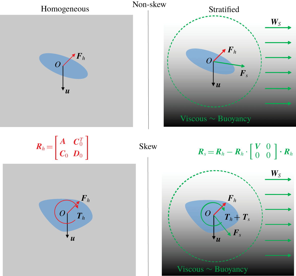
 $$\begin{eqnarray}\unicode[STIX]{x1D64D}_{s}=\unicode[STIX]{x1D64D}_{h}-\unicode[STIX]{x1D64D}_{h}\boldsymbol{\cdot }\left(\begin{array}{@{}cc@{}}\unicode[STIX]{x1D651} & 0\\ 0 & 0\end{array}\right)\boldsymbol{\cdot }\unicode[STIX]{x1D64D}_{h}.\end{eqnarray}$$
Here, we would like to note that expressions for the hydrodynamic force or torque calculated for arbitrary particle shapes are reported in the literature, where the background fluid is homogeneous, the ambient flow is linear (Harper & Chang Reference Harper and Chang1968; Candelier, Mehlig & Magnaudet Reference Candelier, Mehlig and Magnaudet2019) and the small parameter employed in the perturbation scheme is based on the Reynolds number. However, this is the first time that the motion of an arbitrary-shaped particle is investigated in a stratified background fluid.
5 Results and discussion
In this section, we shall analyse the influence of stratification on the force and torque experienced by the particle by considering some specific examples. We divide our analysis into two classes of particles depending on the symmetricity of the particle.
Class (a): non-skew particles – particles which possess a centre of hydrodynamic stress (e.g. orthotropic particles, bodies of revolution, spherically isotropic particles etc.).
Class (b): skew particles – particles which do not possess a centre of hydrodynamic stress.
For both classes of particles, we first analyse general expressions for the force and the torque experienced by the particle. Then, we consider specific examples and derive analytical expressions for the force and and the torque experienced by the particle settling along the density gradient, by considering both the limits of high ( $Pe\gg 1$) and low (
 $Pe\ll 1$) Péclet numbers.
5.1 Class (a): non-skew particles
For this class of particles, we choose the origin ( $O$) to be the centre of hydrodynamic stress. It is known that the coupling tensor (
 $\unicode[STIX]{x1D63E}_{O}$) about the centre of hydrodynamic stress is identically zero. Examples of such particles include spheres, spheroids, ellipsoids, disks or regular polyhedrons. We now use (4.3) to calculate the general expression for the force and torque acting on this class of particles as follows:
 $$\begin{eqnarray}\displaystyle & \displaystyle \boldsymbol{F}=\boldsymbol{F}_{0}-\unicode[STIX]{x1D63C}\boldsymbol{\cdot }\unicode[STIX]{x1D651}\boldsymbol{\cdot }\boldsymbol{F}_{0}, & \displaystyle \nonumber\\ \displaystyle & \displaystyle \boldsymbol{G}=\boldsymbol{G}_{0}. & \displaystyle \nonumber\end{eqnarray}$$
We thus find that although stratification alters the force experienced by the particle, the torque remains unchanged in the presence of stratification (excluding hydrostatic torque). This implies that the hydrodynamic torque induced by stratification is zero. This can be understood by considering that stratification induces a uniform velocity far away from the particle. For a non-skew particle, as there is no coupling between translation and rotation, we expect the torque exerted by this uniform stream of velocity on the particle to be zero. We now simplify the force expression by writing  $\boldsymbol{F}_{0}$ in terms of the Stokes resistance tensors and obtain the following:
 $$\begin{eqnarray}\boldsymbol{F}=(\unicode[STIX]{x1D63C}-\unicode[STIX]{x1D63C}\boldsymbol{\cdot }\unicode[STIX]{x1D651}\boldsymbol{\cdot }\unicode[STIX]{x1D63C})\boldsymbol{\cdot }\boldsymbol{u}.\end{eqnarray}$$
We observe that the tensor  $\unicode[STIX]{x1D63C}-\unicode[STIX]{x1D63C}\boldsymbol{\cdot }\unicode[STIX]{x1D651}\boldsymbol{\cdot }\unicode[STIX]{x1D63C}$ represents the modified translation tensor in the presence of stratification. Thus, for non-skew particles, the only effect stratification has is to modify the translation tensor, while the rotation tensor remains the same. If we denote the modified resistance tensors in the presence of stratification as
 $\unicode[STIX]{x1D63C}^{s},\unicode[STIX]{x1D63F}_{O}^{s}$, we can now write their expressions as
 $$\begin{eqnarray}\unicode[STIX]{x1D63C}^{s}=\unicode[STIX]{x1D63C}-\unicode[STIX]{x1D63C}\boldsymbol{\cdot }\unicode[STIX]{x1D651}\boldsymbol{\cdot }\unicode[STIX]{x1D63C},\quad \unicode[STIX]{x1D63F}_{O}^{s}=\unicode[STIX]{x1D63F}_{O}.\end{eqnarray}$$
For low Péclet numbers ( $Pe\ll 1$), the particle dynamics is governed by the small parameter
 $(RiPe)^{1/4}$. This parameter can be defined as the ratio of characteristic particle length scale (
 $l$) and the stratification length scale
 $l_{s}=(\unicode[STIX]{x1D708}\unicode[STIX]{x1D705}/N^{2})^{1/4}$ (Ardekani & Stocker Reference Ardekani and Stocker2010), where
 $\unicode[STIX]{x1D708}$ is the kinematic viscosity of the fluid,
 $\unicode[STIX]{x1D705}$ is the diffusivity coefficient and
 $N=\sqrt{\unicode[STIX]{x1D6FE}g/\unicode[STIX]{x1D70C}_{\infty }}$ is the Brunt–Väisälä frequency. Here,
 $(RiPe)^{1/4}$ does not have any dependence on the velocity scale (
 $u_{c}$), which implies that convection of the stratifying agent does not contribute to the stratification induced hydrodynamic drag for small Péclet numbers. Consequently,
 $(RiPe)^{1/4}$ can be described a Rayleigh number measuring the relative importance of buoyancy and diffusion.
In order to demonstrate the application of our results, we discuss the dynamics of a rigid particle which is settling in a direction parallel to the density gradient. As discussed before, sedimentation of particles in stratified environments such as oceans or the atmosphere is of physical significance and our analysis will help us obtain crucial insights into this process. We analyse the problem by considering both the limits of high ( $Pe\gg 1$) and low (
 $Pe\ll 1$) Péclet numbers.
5.2 Unidirectional settling in a density stratified fluid
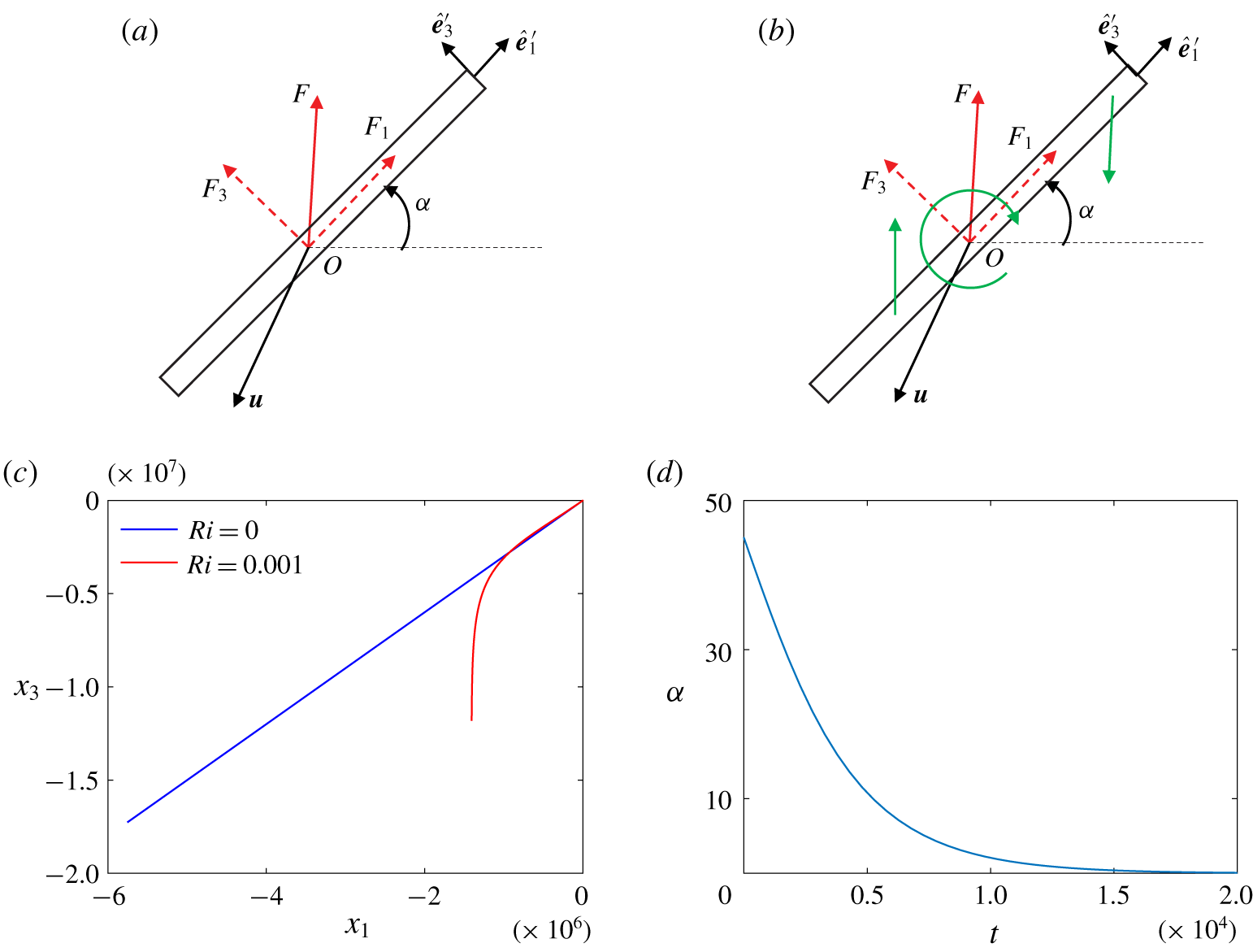
We consider the motion of a non-skew particle, translating with a velocity  $u\hat{\boldsymbol{e}}_{3}$. We choose the coordinate axes fixed in the particle to be the principal axes of translation for the particle (refer to coordinate system
 $(\hat{\boldsymbol{e}}_{1}^{\prime }-\hat{\boldsymbol{e}}_{2}^{\prime }-\hat{\boldsymbol{e}}_{3}^{\prime })$ in figure 1). The origin
 $O$ is the centre of hydrodynamic stress of the body. For simplicity, we assume that the
 $\hat{\boldsymbol{e}}_{2}^{\prime }$ axis of the particle is coincident with the
 $\hat{\boldsymbol{e}}_{2}$ axis, due to which the rotation matrix can be written as
 $$\begin{eqnarray}\unicode[STIX]{x1D64D}=\left[\begin{array}{@{}ccc@{}}\cos (\unicode[STIX]{x1D6FC}) & 0 & -\sin (\unicode[STIX]{x1D6FC})\\ 0 & 1 & 0\\ \sin (\unicode[STIX]{x1D6FC}) & 0 & \cos (\unicode[STIX]{x1D6FC})\end{array}\right],\end{eqnarray}$$
where  $\unicode[STIX]{x1D6FC}$ is the angle between the
 $\hat{\boldsymbol{e}}_{1}^{\prime }$ and
 $\hat{\boldsymbol{e}}_{1}$ axes. The translation tensor for a non-skew particle can be expressed as
 $$\begin{eqnarray}\unicode[STIX]{x1D63C}=\left[\begin{array}{@{}ccc@{}}a_{1} & 0 & 0\\ 0 & a_{2} & 0\\ 0 & 0 & a_{3}\end{array}\right]\!.\end{eqnarray}$$
Here,  $a_{1},a_{2}$ and
 $a_{3}$ are arbitrary constants which depend on the shape of the particle. We emphasize that, for a homogeneous fluid, the translation tensor is independent of the particle’s velocity, orientation and the fluid properties.
(I) High Péclet numbers ( $Pe\gg 1$):
The value of  $\unicode[STIX]{x1D651}^{s}$ is obtained by evaluating the integral in (3.15). For the case considered, the exact expression for
 $\unicode[STIX]{x1D651}^{s}$ is given in appendix B. Here, we numerically evaluate the integral to obtain the following:
 $$\begin{eqnarray}\unicode[STIX]{x1D651}^{s}=-{\displaystyle \frac{Ri^{1/3}}{8\unicode[STIX]{x03C0}^{3}}}\left[\begin{array}{@{}ccc@{}}-1.7436 & 0 & 0\\ 0 & -1.7436 & 0\\ 0 & 0 & -13.9488\end{array}\right]\!.\end{eqnarray}$$
For a sphere moving vertically in a stratified fluid, we substitute the expression for  $\unicode[STIX]{x1D651}^{s}$ in (5.1) to obtain the hydrodynamic force acting on the sphere as follows:
 $$\begin{eqnarray}\boldsymbol{F}=F_{0}\hat{\boldsymbol{e}}_{3}+1.060Ri^{1/3}F_{0}\hat{\boldsymbol{e}}_{3}.\end{eqnarray}$$
This expression matches with that derived by Zvirin & Chadwick (Reference Zvirin and Chadwick1975). Here, it should be emphasized that, while the general expression for  $\unicode[STIX]{x1D651}^{s}$ is independent of the shape of the particle, it depends on the particle velocity (refer to (3.15)). Hence, the expression for
 $\unicode[STIX]{x1D651}^{s}$ obtained above is only valid for particles settling parallel to the density gradient. We now evaluate the tensor
 $\unicode[STIX]{x1D651}$ from (3.16) and calculate the modified translation tensor due to stratification from (5.1) to be as follows:
 $$\begin{eqnarray}\unicode[STIX]{x1D63C}^{s}=\left[\begin{array}{@{}ccc@{}}a_{1}-a_{1}^{2}\,f_{1}(\unicode[STIX]{x1D6FC})Ri^{1/3} & 0 & 0.049a_{1}a_{3}g(\unicode[STIX]{x1D6FC})Ri^{1/3}\\ 0 & a_{2}-0.007a_{2}^{2}Ri^{1/3} & 0\\ 0.049a_{1}a_{3}g(\unicode[STIX]{x1D6FC})Ri^{1/3} & 0 & a_{3}-a_{3}^{2}\,f_{2}(\unicode[STIX]{x1D6FC})Ri^{1/3}\end{array}\right]\!.\end{eqnarray}$$
Here,  $f_{1}(\unicode[STIX]{x1D6FC})=0.007\cos ^{2}\unicode[STIX]{x1D6FC}+0.056\sin ^{2}\unicode[STIX]{x1D6FC},f_{2}(\unicode[STIX]{x1D6FC})=0.007\sin ^{2}\unicode[STIX]{x1D6FC}+0.056\cos ^{2}\unicode[STIX]{x1D6FC}$ and
 $g(\unicode[STIX]{x1D6FC})=\sin \unicode[STIX]{x1D6FC}\cos \unicode[STIX]{x1D6FC}$. We firstly observe that the off-diagonal components of the resistance matrix are non-zero, as opposed to the homogeneous counterpart. This can be understood from (5.2) by expanding the expression for
 $\unicode[STIX]{x1D63C}^{s}$ and by noting that
 $\unicode[STIX]{x1D651}^{s}$ is not isotropic (refer to (5.3)) as the density gradient in the fluid is present only in the vertical direction. Consequently, in addition to the drag, the particle will experience lift forces as well. Additionally, we observe that
 $\unicode[STIX]{x1D651}^{s}$ is independent of the orientation of the particle, which implies that the stratification induced velocity far away from the particle is independent of its orientation (refer to (3.14)). Hence, we expect the modified translation tensor to be independent of the particle orientation, as in the case of a homogeneous fluid (refer to (3.14)).
For  $\unicode[STIX]{x1D6FC}=0$,
 $g(\unicode[STIX]{x1D6FC})=0$ and the off-diagonal components of the modified translation tensor are zero. This implies that the principal axes of translation of the particle remain the same in the presence of stratification when one of the principal axes of translation coincides with the gravity direction. However, for
 $\unicode[STIX]{x1D6FC}\neq 0$,
 $\unicode[STIX]{x1D63C}^{s}$ is not diagonal and we expect the principal axes of translation of the particle to be modified due to stratification. We now evaluate the eigen vectors of
 $\unicode[STIX]{x1D63C}^{s}$ to find the modified principal axes of translation for non-zero
 $\unicode[STIX]{x1D6FC}$ as follows:
 $$\begin{eqnarray}\hat{\boldsymbol{e}}_{1}^{s}=\hat{\boldsymbol{e}}_{1}^{\prime }+m_{1}\hat{\boldsymbol{e}}_{3}^{\prime },\quad \hat{\boldsymbol{e}}_{2}^{s}=\hat{\boldsymbol{e}}_{2}^{\prime },\quad \hat{\boldsymbol{e}}_{3}^{s}=m_{2}\hat{\boldsymbol{e}}_{1}^{\prime }+\hat{\boldsymbol{e}}_{3}^{\prime }.\end{eqnarray}$$
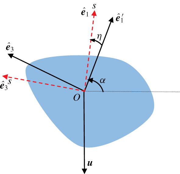
Modified principal axes of translation (depicted by dashed red lines) in the presence of stratification. Here,  $O$ is the centre of hydrodynamic stress.

Here,  $m_{1}=-\unicode[STIX]{x1D6FC}_{1}-\unicode[STIX]{x1D6FC}_{3}-\sqrt{(\unicode[STIX]{x1D6FC}_{1}-\unicode[STIX]{x1D6FC}_{3})^{2}+4\unicode[STIX]{x1D6FD}_{1}^{2}}/2\unicode[STIX]{x1D6FD}_{1}$ and
 $m_{2}=-2\unicode[STIX]{x1D6FD}_{1}/\unicode[STIX]{x1D6FC}_{1}-\unicode[STIX]{x1D6FC}_{3}+\sqrt{(\unicode[STIX]{x1D6FC}_{1}-\unicode[STIX]{x1D6FC}_{3})^{2}+4\unicode[STIX]{x1D6FD}_{1}^{2}}$, where,
 $\unicode[STIX]{x1D6FC}_{1}=a_{1}-a_{1}^{2}\,f_{1}(\unicode[STIX]{x1D6FC})Ri^{1/3}$,
 $\unicode[STIX]{x1D6FC}_{3}=a_{3}-a_{3}^{2}\,f_{2}(\unicode[STIX]{x1D6FC})Ri^{1/3}$ and
 $\unicode[STIX]{x1D6FD}_{1}=0.049a_{1}a_{3}g(\unicode[STIX]{x1D6FC})Ri^{1/3}$. The modified principal axes are schematically shown in figure 2, where the angle
 $\unicode[STIX]{x1D702}$ is given by
 $$\begin{eqnarray}\unicode[STIX]{x1D702}=\cos ^{-1}\left({\displaystyle \frac{1}{\sqrt{1+m_{1}^{2}}}}\right).\end{eqnarray}$$
In order to calculate the modified principal translational resistances of the particle, we calculate the eigen values of the tensor  $\unicode[STIX]{x1D63C}^{s}$ to be as follows:
 $$\begin{eqnarray}\displaystyle & \displaystyle e_{1}={\textstyle \frac{1}{2}}\left(\unicode[STIX]{x1D6FC}_{1}+\unicode[STIX]{x1D6FC}_{3}+\sqrt{(\unicode[STIX]{x1D6FC}_{1}-\unicode[STIX]{x1D6FC}_{3})^{2}+4\unicode[STIX]{x1D6FD}_{1}^{2}}\right),\quad e_{2}=a_{2}-0.007a_{2}^{2}Ri^{1/3}, & \displaystyle \nonumber\\ \displaystyle & \displaystyle e_{3}={\textstyle \frac{1}{2}}\left(\unicode[STIX]{x1D6FC}_{1}+\unicode[STIX]{x1D6FC}_{3}-\sqrt{(\unicode[STIX]{x1D6FC}_{1}-\unicode[STIX]{x1D6FC}_{3})^{2}+4\unicode[STIX]{x1D6FD}_{1}^{2}}\right). & \displaystyle \nonumber\end{eqnarray}$$
Here,  $e_{1},e_{2},e_{3}$ are the eigen values of tensor
 $\unicode[STIX]{x1D63C}^{s}$. We know that
 $a_{i}<0$ for
 $i=\{1,2,3\}$ as the force exerted on a particle moving through a homogeneous fluid always acts in a direction opposing its motion. Now, from the eigenvalue expressions, we can observe that
 $|e_{2}|\geqslant |a_{2}|$. It can be easily shown that
 $|e_{1}|\geqslant |\unicode[STIX]{x1D6FC}_{1}|$ and
 $|e_{3}|\geqslant |\unicode[STIX]{x1D6FC}_{3}|$ by squaring both the sides of the expressions. Additionally, we observe that
 $|\unicode[STIX]{x1D6FC}_{1}|\geqslant |a_{1}|$ and
 $|\unicode[STIX]{x1D6FC}_{3}|\geqslant |a_{3}|$. From the above observations, we infer that
 $|e_{1}|\geqslant |a_{1}|$ and
 $|e_{3}|\geqslant |a_{3}|$. This implies that stratification increases the magnitude of the principal translational resistances of the particle.
We now proceed to calculate the modified translation tensors for some particles for which the translation tensors are known, to demonstrate the application of our derivation. We consider  $\unicode[STIX]{x1D6FC}=0$ in the following examples, which corresponds to the case where the principal axes of the particle are parallel to the laboratory fixed axes. However, it should be noted that more general expressions in terms of
 $\unicode[STIX]{x1D6FC}$ can be easily derived using (5.4).
(a) Thin circular disk:
For thin circular disks, with the circular cross-section parallel to the  $\hat{\boldsymbol{e}}_{1}$–
 $\hat{\boldsymbol{e}}_{3}$ plane, we have
 $a_{1}=-32/3,a_{2}=-16$ and
 $a_{3}=-32/3$ (Brenner Reference Brenner1963). We apply our results to obtain the modified translation tensor for the disk moving through a stratified field as follows:
 $$\begin{eqnarray}\unicode[STIX]{x1D63C}^{s}=\left[\begin{array}{@{}ccc@{}}-{\textstyle \frac{32}{3}}-0.796Ri^{1/3} & 0 & 0\\ 0 & -16-1.792Ri^{1/3} & 0\\ 0 & 0 & -{\textstyle \frac{32}{3}}-6.37Ri^{1/3}\end{array}\right]\!.\end{eqnarray}$$
(b) Prolate spheroids:
For the case of prolate spheroids with the longer axis parallel to the  $\hat{\boldsymbol{e}}_{3}$ axis, we can write,
 $a_{1}=a_{2}=-32\unicode[STIX]{x03C0}e^{3}(2e+(3e^{2}-1)\log (1+e/1-e))^{-1},a_{3}=-16\unicode[STIX]{x03C0}e^{3}(-2e+(1+e^{2})\log (1+e/1-e))^{-1}$ (Kim & Karrila Reference Kim and Karrila2013), where
 $e$ is the eccentricity ratio of the spheroid. We now use (5.4) to obtain the modified coefficients of the translation tensor as follows:
 $$\begin{eqnarray}\displaystyle \displaystyle a_{1}^{s} & = & \displaystyle -32\unicode[STIX]{x03C0}e^{3}\left(2e+(3e^{2}-1)\log \left({\displaystyle \frac{1+e}{1-e}}\right)\right)^{-1}\nonumber\\ \displaystyle & & \displaystyle -\,70.7Ri^{1/3}e^{6}\left(2e+(3e^{2}-1)\log \left({\displaystyle \frac{1+e}{1-e}}\right)\right)^{-2},\nonumber\\ \displaystyle \displaystyle a_{2}^{s} & = & \displaystyle -32\unicode[STIX]{x03C0}e^{3}\left(2e+(3e^{2}-1)\log \left({\displaystyle \frac{1+e}{1-e}}\right)\right)^{-1}\nonumber\\ \displaystyle & & \displaystyle -\,70.7Ri^{1/3}e^{6}\left(2e+(3e^{2}-1)\log \left({\displaystyle \frac{1+e}{1-e}}\right)\right)^{-2},\nonumber\\ \displaystyle \displaystyle a_{3}^{s} & = & \displaystyle -16\unicode[STIX]{x03C0}e^{3}\left(-2e+(1+e^{2})\log \left({\displaystyle \frac{1+e}{1-e}}\right)\right)^{-1}\nonumber\\ \displaystyle & & \displaystyle -\,141.49Ri^{1/3}e^{6}\left(-2e+(1+e^{2})\log \left({\displaystyle \frac{1+e}{1-e}}\right)\right)^{-2}.\nonumber\end{eqnarray}$$
(c) Weakly deformed spheres:
Particles encountered in nature and in industrial applications often have irregular shapes which cannot be expressed in a simple coordinate system. As an example of particles having irregular shapes, Brenner (Reference Brenner1963) considered slightly deformed spheres and derived general expressions for the Stokes resistance tensors for these particles. The surface of these particles is described by,  $r=1+\unicode[STIX]{x1D6FD}h(\unicode[STIX]{x1D703},\unicode[STIX]{x1D719})$, where
 $\unicode[STIX]{x1D6FD}\ll 1$ and
 $r,\unicode[STIX]{x1D703},\unicode[STIX]{x1D719}$ are spherical coordinates with the origin at the centre of the undeformed sphere. Here,
 $\unicode[STIX]{x1D6FD}$ signifies the extent of deviation from the spherical geometry. The function
 $h$ is expressed as a sum of surface spherical harmonics,
 $h_{k}(\unicode[STIX]{x1D703},\unicode[STIX]{x1D719})$. The translation tensor derived by Brenner (Reference Brenner1963) for this particle is given by
 $$\begin{eqnarray}\unicode[STIX]{x1D63C}=-6\unicode[STIX]{x03C0}\left(\unicode[STIX]{x1D644}+\unicode[STIX]{x1D6FD}(\unicode[STIX]{x1D644}h_{0}-{\textstyle \frac{1}{10}}\unicode[STIX]{x1D735}\unicode[STIX]{x1D735}(r^{2}h_{2}))+O(\unicode[STIX]{x1D6FD}^{2})\right).\end{eqnarray}$$
We can substitute this expression in (5.2) to calculate the modified translation tensor for a general weakly deformed sphere up to first order in  $\unicode[STIX]{x1D6FD}$. In order to illustrate the application of our method, we now evaluate the modified translation tensor for a weakly deformed sphere in the shape of a spheroid (
 $h=-\cos ^{2}\unicode[STIX]{x1D703}$). We use equation (5.6) to obtain the coefficients of the translation tensor up to first order in
 $\unicode[STIX]{x1D6FD}$ as,
 $a_{1}=-6\unicode[STIX]{x03C0}+2.4\unicode[STIX]{x03C0}\unicode[STIX]{x1D6FD},a_{2}=-6\unicode[STIX]{x03C0}+2.4\unicode[STIX]{x03C0}\unicode[STIX]{x1D6FD}$ and
 $a_{3}=-6\unicode[STIX]{x03C0}+1.2\unicode[STIX]{x03C0}\unicode[STIX]{x1D6FD}$ (Brenner Reference Brenner1963). Using (5.4), we obtain the coefficients of the modified translation tensor as follows:
 $$\begin{eqnarray}\displaystyle & \displaystyle a_{1}^{s}=-6\unicode[STIX]{x03C0}+2.4\unicode[STIX]{x1D6FD}\unicode[STIX]{x03C0}+Ri^{1/3}(-2.48+1.99\unicode[STIX]{x1D6FD})+O(\unicode[STIX]{x1D6FD}^{2}), & \displaystyle \nonumber\\ \displaystyle & \displaystyle a_{2}^{s}=-6\unicode[STIX]{x03C0}+2.4\unicode[STIX]{x1D6FD}\unicode[STIX]{x03C0}+Ri^{1/3}(-2.48+1.99\unicode[STIX]{x1D6FD})+O(\unicode[STIX]{x1D6FD}^{2}), & \displaystyle \nonumber\\ \displaystyle & \displaystyle a_{3}^{s}=-6\unicode[STIX]{x03C0}+1.2\unicode[STIX]{x1D6FD}\unicode[STIX]{x03C0}+Ri^{1/3}(-19.8+7.96\unicode[STIX]{x1D6FD})+O(\unicode[STIX]{x1D6FD}^{2}). & \displaystyle \nonumber\end{eqnarray}$$
A high value of  $Pe$ and low value of
 $Re$ corresponds to a fluid which has a high Prandtl number. Hence, the results of this section would be applicable for fluids which have high values of Prandtl number, such as salt stratified water or temperature stratified viscous oils or greases (
 $Pr\sim 10^{3}-10^{6}$) (Leal Reference Leal2007).
(II) Low Péclet numbers ( $Pe\ll 1$):
For particles settling parallel to the density gradient, we numerically evaluate the matrix  $\unicode[STIX]{x1D651}^{s}$ for the case of low Péclet numbers to be as follows (the exact expression is provided in appendix B). The components of
 $\unicode[STIX]{x1D651}^{s}$ were also reported by Candelier et al. (Reference Candelier, Mehaddi and Vauquelin2014) in the context of a sphere translating through a stratified fluid at low Péclet numbers. We obtain the following:
 $$\begin{eqnarray}\unicode[STIX]{x1D651}^{s}=-{\displaystyle \frac{Ri^{1/4}Pe^{1/4}}{8\unicode[STIX]{x03C0}^{3}}}\left[\begin{array}{@{}ccc@{}}-1.7427 & 0 & 0\\ 0 & -1.74327 & 0\\ 0 & 0 & -8.7138\end{array}\right]\!.\end{eqnarray}$$
We again calculate the force experienced by a vertically translating sphere in this limit and obtain the following expression:
 $$\begin{eqnarray}\boldsymbol{F}=F_{0}\hat{\boldsymbol{e}}_{3}+0.662(RiPe)^{1/4}F_{0}\hat{\boldsymbol{e}}_{3}.\end{eqnarray}$$
This expression matches with that derived by Candelier et al. (Reference Candelier, Mehaddi and Vauquelin2014). The expression for the modified translation tensor can be determined to be as follows:
 $$\begin{eqnarray}\unicode[STIX]{x1D63C}^{s}=\left[\begin{array}{@{}ccc@{}}a_{1}-a_{1}^{2}\,f_{1}(\unicode[STIX]{x1D6FC})(RiPe)^{1/4} & 0 & 0.028a_{1}a_{3}g(\unicode[STIX]{x1D6FC})(RiPe)^{1/4}\\ 0 & a_{2}-0.007a_{2}^{2}(RiPe)^{1/4} & 0\\ 0.028a_{1}a_{3}g(\unicode[STIX]{x1D6FC})(RiPe)^{1/4} & 0 & a_{3}-a_{3}^{2}\,f_{2}(\unicode[STIX]{x1D6FC})(RiPe)^{1/4}\end{array}\right]\!.\end{eqnarray}$$
Here,  $f_{1}(\unicode[STIX]{x1D6FC})=0.007\cos ^{2}\unicode[STIX]{x1D6FC}+0.035\sin ^{2}\unicode[STIX]{x1D6FC}$,
 $f_{2}(\unicode[STIX]{x1D6FC})=0.007\sin ^{2}\unicode[STIX]{x1D6FC}+0.035\cos ^{2}\unicode[STIX]{x1D6FC}$ and
 $g(\unicode[STIX]{x1D6FC})=\sin \unicode[STIX]{x1D6FC}\cos \unicode[STIX]{x1D6FC}$. The structure of the modified translation tensor is similar to that obtained for high Péclet numbers (refer to (5.4)). Consequently, we again expect the principal axes of translation to be modified in the presence of stratification for non-zero
 $\unicode[STIX]{x1D6FC}$. We expect similar expressions for the modified principal axes of translation as provided in (5.5), with the parameter
 $Ri^{1/3}$ being replaced by
 $(RiPe)^{1/4}$. As in the case of high Péclet numbers, we expect that stratification enhances the magnitude of the principal translational resistances of the particle.
For both the cases of high and low Péclet numbers, the coefficients of stratification induced drag given by  $Ri^{1/3}$ and
 $(RiPe)^{1/4}$ are proportional to the characteristic length scale of the particle (
 $l_{c}$). Hence, as opposed to the drag force in a homogeneous fluid which is proportional to
 $l_{c}$, the leading-order stratification induced drag scales as the second power of the characteristic particle dimension (
 $F_{stratification}\sim l_{c}^{2}$).
We again consider the examples of a circular disk, prolate spheroid and a weakly deformed sphere settling along the density gradient in a stratified fluid for  $\unicode[STIX]{x1D6FC}=0$ and calculate the modified translation tensors in each case.
(a) Thin circular disk:
We obtain the following modified translation tensor for the settling of a thin circular disk at low Péclet numbers:
 $$\begin{eqnarray}\unicode[STIX]{x1D63C}^{s}=\left[\begin{array}{@{}ccc@{}}-{\textstyle \frac{32}{3}}-0.796(RiPe)^{1/4} & 0 & 0\\ 0 & -16-1.792(RiPe)^{1/4} & 0\\ 0 & 0 & -{\textstyle \frac{32}{3}}-3.98(RiPe)^{1/4}\end{array}\right]\!.\end{eqnarray}$$
For temperature stratified water ( $Pr=7$), the Péclet number for slow moving particles (
 $Re\ll 1$) is almost negligible. We note that plastic pellets in the form of disks of flattened cylinders (Turner & Holmes Reference Turner and Holmes2011) are a major constituent of debris in oceans. We can thus apply our results to study sedimentation rates of plastic disks in temperature stratified water or even disc shaped particles settling in gaseous environments for which
 $Pr$ is usually small. From the modified translation tensor (
 $\unicode[STIX]{x1D63C}^{s}$), we observe that the maximum drag increase occurs in the direction of stratification with a magnitude of
 ${\approx}4(RiPe)^{1/4}$.
(b) Prolate spheroids:
We obtain the coefficients of the modified translation tensor for a prolate spheroid sedimenting at low Péclet numbers as follows:
 $$\begin{eqnarray}\displaystyle a_{1}^{s} & = & \displaystyle -32\unicode[STIX]{x03C0}e^{3}\left(2e+(3e^{2}-1)\log \left({\displaystyle \frac{1+e}{1-e}}\right)\right)^{-1}\nonumber\\ \displaystyle & & \displaystyle -\,70.7(RiPe)^{1/4}e^{6}\left(2e+(3e^{2}-1)\log \left({\displaystyle \frac{1+e}{1-e}}\right)\right)^{-2},\nonumber\\ \displaystyle a_{2}^{s} & = & \displaystyle -32\unicode[STIX]{x03C0}e^{3}\left(2e+(3e^{2}-1)\log \left({\displaystyle \frac{1+e}{1-e}}\right)\right)^{-1}\nonumber\\ \displaystyle & & \displaystyle -\,70.7(RiPe)^{1/4}e^{6}\left(2e+(3e^{2}-1)\log \left({\displaystyle \frac{1+e}{1-e}}\right)\right)^{-2},\nonumber\\ \displaystyle a_{3}^{s} & = & \displaystyle -16\unicode[STIX]{x03C0}e^{3}\left(-2e+(1+e^{2})\log \left({\displaystyle \frac{1+e}{1-e}}\right)\right)^{-1}\nonumber\\ \displaystyle & & \displaystyle -\,88.43(RiPe)^{1/4}e^{6}\left(-2e+(1+e^{2})\log \left({\displaystyle \frac{1+e}{1-e}}\right)\right)^{-2}.\nonumber\end{eqnarray}$$
Most of the marine phytoplankton in the oceans are not spherical, and more frequently have a needle or rod shaped geometry in which the aspect ratio is much greater than 1 (Bainbridge Reference Bainbridge1957). We can apply our results for the low Péclet regime to study settling of needle/rod shaped organisms ( $e\rightarrow 1$) in temperature stratified water. We evaluate the drag coefficients for
 $e=0.99$ and obtain the following matrix:
 $$\begin{eqnarray}\unicode[STIX]{x1D63C}^{s}=\left[\begin{array}{@{}ccc@{}}-7.96-0.44(RiPe)^{1/4} & 0 & 0\\ 0 & -7.96-0.44(RiPe)^{1/4} & 0\\ 0 & 0 & -5.7-1.15(RiPe)^{1/4}\end{array}\right]\!.\end{eqnarray}$$
We obtain a maximum drag increase of  $1.15(RiPe)^{1/4}$ in the direction parallel to the density gradient. For
 $Ri=10^{-1},Pe=10^{-2}$, this corresponds to an increase in drag of almost
 $4\%$.
(c) Weakly deformed spheres:
The translation tensor for a weakly deformed sphere translating in a homogeneous fluid is given by (5.6). As in the case for high  $Pe$, we consider the example of a weakly deformed sphere in the shape of a spheroid. We use (5.8) to obtain the coefficients of the modified translation tensor as follows:
 $$\begin{eqnarray}\displaystyle & \displaystyle a_{1}^{s}=-6\unicode[STIX]{x03C0}+2.4\unicode[STIX]{x1D6FD}\unicode[STIX]{x03C0}+(RiPe)^{1/4}(-2.48+1.99\unicode[STIX]{x1D6FD})+O(\unicode[STIX]{x1D6FD}^{2}), & \displaystyle \nonumber\\ \displaystyle & \displaystyle a_{2}^{s}=-6\unicode[STIX]{x03C0}+2.4\unicode[STIX]{x1D6FD}\unicode[STIX]{x03C0}+(RiPe)^{1/4}(-2.48+1.99\unicode[STIX]{x1D6FD})+O(\unicode[STIX]{x1D6FD}^{2}), & \displaystyle \nonumber\\ \displaystyle & \displaystyle a_{3}^{s}=-6\unicode[STIX]{x03C0}+1.2\unicode[STIX]{x1D6FD}\unicode[STIX]{x03C0}+(RiPe)^{1/4}(-12.37+4.97\unicode[STIX]{x1D6FD})+O(\unicode[STIX]{x1D6FD}^{2}). & \displaystyle \nonumber\end{eqnarray}$$
The magnitude of stratification is often described by the Brunt–Väisälä frequency ( $N=\sqrt{\unicode[STIX]{x1D6FE}g/\unicode[STIX]{x1D70C}_{\infty }}$). We note that the typical values of
 $N$ are in the range
 $10^{-4}-0.3$
 $s^{-1}$ (Thorpe Reference Thorpe2005). Using this estimate, in density stratified water (
 $\unicode[STIX]{x1D70C}_{\infty }\approx 1000~\text{kg}~\text{m}^{-3}$,
 $\unicode[STIX]{x1D707}\approx 10^{-3}~\text{kg}~\text{m}^{-1}~\text{s}^{-1}$), we find that
 $\unicode[STIX]{x1D6FE}\approx 10^{-6}$–
 $10~\text{kg}~\text{m}^{-4}$. We now estimate the typical values of
 $Ri$ and
 $Re$ for slowly sedimenting particles (
 $u_{c}\approx 1~\text{mm}~\text{s}^{-1}$) in density stratified water with
 $\unicode[STIX]{x1D6FE}=1~\text{kg}~\text{m}^{-4}$. Examples include microparticles (
 $l_{c}\approx 1$–
 $100~\unicode[STIX]{x03BC}\text{m}$,
 $Ri\approx 10^{-5}$,
 $Re\approx 10^{-3}$), organic particles such as bacteria (
 $l_{c}\approx 1~\unicode[STIX]{x03BC}\text{m}$,
 $Ri\approx 10^{-10}$,
 $Re\approx 10^{-3}$) and phytoplankton (
 $l_{c}\approx 10{-}100~\unicode[STIX]{x03BC}\text{m}$,
 $Ri\approx 10^{-5}$,
 $Re\approx 10^{-2}$). We can apply our results to understand the settling of such arbitrarily shaped particles. Here, we again note that for larger values of
 $Re$, inertia effects may dominate and our analysis is quantitatively valid for cases where the condition
 $Re\ll Ri^{1/3}$ or
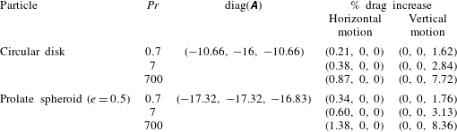
 $Re\ll (RiPe)^{1/4}$ is satisfied depending on whether the Péclet number is large or small, respectively. Table 1 shows the drag increase due to stratification reported for
 $Ri=0.001,Re=0.001$ and for various values of
 $Pr$. We have considered the cases of horizontal motion (
 $\boldsymbol{u}=u\hat{\boldsymbol{e}}_{1}$) and vertical motion (
 $\boldsymbol{u}=u\hat{\boldsymbol{e}}_{3}$). The exact value of Prandtl number is a function of pressure and temperature and the values,
 $Pr=7$ and
 $Pr=700$ correspond to the cases of temperature stratified water at
 $18\,^{\circ }\text{C}$ and salt stratified water, respectively. As we have considered
 $\unicode[STIX]{x1D6FC}=0$, the off-diagonal components of the modified translation tensor would be zero (refer to (5.4)) and the principal axes of the particle would not be modified in the presence of stratification. Consequently, for the cases of horizontal and vertical motions considered, the drag force would lie along the
 $\hat{\boldsymbol{e}}_{1}$ and
 $\hat{\boldsymbol{e}}_{3}$ axes, respectively. We observe that, for particles settling along the density gradient, the drag enhancement is maximum, as expected. For
 $Ri=0.001$ and
 $Re=0.001$, we find that, for temperature stratified water, this drag enhancement is
 ${\approx}3\%$ for circular disks and prolate spheroids. The drag force increases for salt stratification, where the maximum drag enhancement is
 ${\approx}8\%$.
The  $\%$ drag increase due to stratification for
 $Ri=10^{-3},Re=10^{-3}$ and
 $\unicode[STIX]{x1D6FC}=0$.

5.3 Class (b): skew particles
This is a class of particles which do not have a centre of hydrodynamic stress. Hence, irrespective of the choice of the origin  $O$, the coupling tensor will be non-zero (Brenner Reference Brenner1964). Thus, we can write the general expression for the force and the torque experienced by a particle belonging to this class as described in (4.3). We now express
 $\boldsymbol{F}_{0},\boldsymbol{G}_{0}$ in terms of the Stokes resistance tensors and substitute in (4.3) to obtain the following:
 $$\begin{eqnarray}\displaystyle & \displaystyle \boldsymbol{F}=(\unicode[STIX]{x1D63C}-\unicode[STIX]{x1D63C}\boldsymbol{\cdot }\unicode[STIX]{x1D651}\boldsymbol{\cdot }\unicode[STIX]{x1D63C})\boldsymbol{\cdot }\boldsymbol{u}+(\unicode[STIX]{x1D63E}_{O}^{\text{T}}-\unicode[STIX]{x1D63C}\boldsymbol{\cdot }\unicode[STIX]{x1D651}\boldsymbol{\cdot }\unicode[STIX]{x1D63E}_{O}^{\text{T}})\boldsymbol{\cdot }\unicode[STIX]{x1D734}, & \displaystyle\end{eqnarray}$$
 $$\begin{eqnarray}\displaystyle & \displaystyle \boldsymbol{G}=(\unicode[STIX]{x1D63E}_{O}-\unicode[STIX]{x1D63E}_{O}\boldsymbol{\cdot }\unicode[STIX]{x1D651}\boldsymbol{\cdot }\unicode[STIX]{x1D63C})\boldsymbol{\cdot }\boldsymbol{u}+(\unicode[STIX]{x1D63F}_{O}-\unicode[STIX]{x1D63E}_{O}\boldsymbol{\cdot }\unicode[STIX]{x1D651}\boldsymbol{\cdot }\unicode[STIX]{x1D63E}_{O}^{\text{T}})\boldsymbol{\cdot }\unicode[STIX]{x1D734}. & \displaystyle\end{eqnarray}$$
We observe that, for this type of particle, along with the force, stratification induces a non-zero hydrodynamic torque because of the asymmetry in the geometry of the particle, in contrast to the class (a) counterpart. We additionally note that all the Stokes resistance tensors will be modified in the presence of stratification as follows:
 $$\begin{eqnarray}\displaystyle & \displaystyle \unicode[STIX]{x1D63C}^{s}=\unicode[STIX]{x1D63C}-\unicode[STIX]{x1D63C}\boldsymbol{\cdot }\unicode[STIX]{x1D651}\boldsymbol{\cdot }\unicode[STIX]{x1D63C}\quad \unicode[STIX]{x1D63F}_{O}^{s}=\unicode[STIX]{x1D63F}_{O}-\unicode[STIX]{x1D63E}_{O}\boldsymbol{\cdot }\unicode[STIX]{x1D651}\boldsymbol{\cdot }\unicode[STIX]{x1D63E}_{O}^{\text{T}}, & \displaystyle\end{eqnarray}$$
 $$\begin{eqnarray}\displaystyle & \displaystyle \unicode[STIX]{x1D63E}_{O}^{s}=\unicode[STIX]{x1D63E}_{O}-\unicode[STIX]{x1D63E}_{O}\boldsymbol{\cdot }\unicode[STIX]{x1D651}\boldsymbol{\cdot }\unicode[STIX]{x1D63C}. & \displaystyle\end{eqnarray}$$
 $(RiPe)^{1/4}$.
From the expressions for the force and torque, we note that the coupling tensors are still related by the transpose of each other, even though the fluid is not homogeneous. Additionally, as in the case of a homogeneous fluid, we also find that the relations,  $\unicode[STIX]{x1D63C}^{s}=(\unicode[STIX]{x1D63C}^{s})^{\text{T}}$ and
 $\unicode[STIX]{x1D63F}_{O}^{s}=(\unicode[STIX]{x1D63F}_{O}^{s})^{\text{T}}$ are satisfied. It can be easily shown that these relations are satisfied for non-skew particles as well. We shall now consider an example involving settling of a particle belonging to this class, in a direction parallel to the density gradient for both the cases of high (
 $Pe\gg 1$) and low (
 $Pe\ll 1$) Péclet numbers.
Unidirectional settling in a density stratified fluid
(a) Screw propeller system translating with a velocity  $u\hat{\boldsymbol{e}}_{3}$ and (b) side view showing the separation between the planes of the disks by an angle
 $2\unicode[STIX]{x1D703}$;
 $O$ denotes the midpoint of the connecting rod between the two disks.

We consider the example of a screw propeller system, which consists of two infinitesimally thin circular disks joined by a rigid rod of negligible hydrodynamic resistance (refer to figure 3). The radius of each disk is  $c$ and the centre-to-centre spacing between the disks is
 $2h$. The angle between the planes of the disks is
 $2\unicode[STIX]{x1D703}$,
 $0\leqslant \unicode[STIX]{x1D703}\leqslant \unicode[STIX]{x03C0}/2$. We consider that this system is settling with a velocity
 $u\hat{\boldsymbol{e}}_{3}$, with the connecting rod parallel to the
 $\hat{\boldsymbol{e}}_{1}$ axis. We choose the origin to be located at the midpoint of the connecting rod (denoted by
 $O$ in figure 3), with the body fixed axes parallel to the laboratory fixed coordinate axes (
 $\hat{\boldsymbol{e}}_{1},\hat{\boldsymbol{e}}_{2},\hat{\boldsymbol{e}}_{3}$). The resistance tensors for this screw propeller system were derived by Happel & Brenner (Reference Happel and Brenner1981) by superimposing the resistance matrices for the individual disks. They assumed that the disks are sufficiently far apart such that the hydrodynamic interaction between the disks is zero (
 $c/h\ll 1$) and that the resistance of the connecting rod is zero. They obtained the following:
 $$\begin{eqnarray}\displaystyle & \displaystyle \unicode[STIX]{x1D63C}=-{\displaystyle \frac{32c}{3}}\left[\begin{array}{@{}ccc@{}}2 & 0 & 0\\ 0 & 2+\sin ^{2}\unicode[STIX]{x1D703} & 0\\ 0 & 0 & 2+\cos ^{2}\unicode[STIX]{x1D703}\end{array}\right]\!, & \displaystyle \nonumber\\ \displaystyle & \displaystyle \unicode[STIX]{x1D63F}_{O}=-{\displaystyle \frac{32c}{3}}\left[\begin{array}{@{}ccc@{}}2c^{2} & 0 & 0\\ 0 & h^{2}(2+\cos ^{2}\unicode[STIX]{x1D703}) & 0\\ 0 & 0 & h^{2}(2+\sin ^{2}\unicode[STIX]{x1D703})\end{array}\right]\!, & \displaystyle \nonumber\\ \displaystyle & \displaystyle \unicode[STIX]{x1D63E}_{O}=-{\displaystyle \frac{32ch}{3}}\left[\begin{array}{@{}ccc@{}}0 & 0 & 0\\ 0 & -\sin \unicode[STIX]{x1D703}\cos \unicode[STIX]{x1D703} & 0\\ 0 & 0 & \sin \unicode[STIX]{x1D703}\cos \unicode[STIX]{x1D703}\end{array}\right]\!. & \displaystyle \nonumber\end{eqnarray}$$
As the coupling tensor is non-zero, stratification will induce an additional hydrodynamic torque on the particle. We now calculate the modified resistance tensors for this particle by considering the cases of both high and low Péclet numbers.
(a) High Péclet numbers ( $Pe\gg 1$):
We note that, for this case, the expression for  $\unicode[STIX]{x1D651}^{s}$ remains unchanged (refer to (5.3)). We now use the general expression for the modified resistance tensors given in (5.11) to obtain the following:
 $$\begin{eqnarray}\displaystyle & \displaystyle \unicode[STIX]{x1D63C}^{s}=\left[\begin{array}{@{}ccc@{}}-{\displaystyle \frac{64c}{3}}-3.18Ri^{1/3}c^{2} & 0 & 0\\ 0 & -{\displaystyle \frac{32c}{3}}p_{1}(\unicode[STIX]{x1D703})-0.79Ri^{1/3}c^{2}p_{1}^{2}(\unicode[STIX]{x1D703}) & 0\\ 0 & 0 & -{\displaystyle \frac{32c}{3}}p_{2}(\unicode[STIX]{x1D703})-6.37Ri^{1/3}c^{2}p_{2}^{2}(\unicode[STIX]{x1D703})\end{array}\right]\!, & \displaystyle \nonumber\\ \displaystyle & \displaystyle \unicode[STIX]{x1D63F}_{O}^{s}=\left[\begin{array}{@{}ccc@{}}-{\displaystyle \frac{64c^{3}}{3}} & 0 & 0\\ 0 & -{\displaystyle \frac{32c}{3}}h^{2}p_{2}(\unicode[STIX]{x1D703})-0.79Ri^{1/3}c^{2}h^{2}p_{3}^{2}(\unicode[STIX]{x1D703}) & 0\\ 0 & 0 & -{\displaystyle \frac{32c}{3}}h^{2}p_{1}(\unicode[STIX]{x1D703})-6.37Ri^{1/3}c^{2}h^{2}p_{3}^{2}(\unicode[STIX]{x1D703})\end{array}\right]\!, & \displaystyle \nonumber\\ \displaystyle & \displaystyle \unicode[STIX]{x1D63E}_{O}^{s}=\left[\begin{array}{@{}ccc@{}}0 & 0 & 0\\ 0 & {\displaystyle \frac{32ch}{3}}p_{3}(\unicode[STIX]{x1D703})+0.79Ri^{1/3}c^{2}hp_{1}(\unicode[STIX]{x1D703})p_{3}(\unicode[STIX]{x1D703}) & 0\\ 0 & 0 & -{\displaystyle \frac{32ch}{3}}p_{3}(\unicode[STIX]{x1D703})-6.37Ri^{1/3}c^{2}hp_{2}(\unicode[STIX]{x1D703})p_{3}(\unicode[STIX]{x1D703})\end{array}\right]\!. & \displaystyle \nonumber\end{eqnarray}$$
Here,  $p_{1}(\unicode[STIX]{x1D703})=2+\sin ^{2}\unicode[STIX]{x1D703}$,
 $p_{2}(\unicode[STIX]{x1D703})=2+\cos ^{2}\unicode[STIX]{x1D703}$ and
 $p_{3}(\unicode[STIX]{x1D703})=\sin \unicode[STIX]{x1D703}\cos \unicode[STIX]{x1D703}$. From the expression for
 $\unicode[STIX]{x1D63C}^{s}$, we again observe that stratification augments the drag force acting on the particle. As we have considered unidirectional settling parallel to the
 $\hat{\boldsymbol{e}}_{3}$ direction, stratification induced hydrodynamic torque can be calculated from the expression of the coupling tensor as
 $$\begin{eqnarray}\boldsymbol{G}_{stratified}=-6.37Ri^{1/3}c^{2}h(2\sin \unicode[STIX]{x1D703}\cos \unicode[STIX]{x1D703}+\sin \unicode[STIX]{x1D703}\cos ^{3}\unicode[STIX]{x1D703})u\hat{\boldsymbol{e}}_{3}.\end{eqnarray}$$
(b) Low Péclet numbers ( $Pe\ll 1$):
Using the expression for  $\unicode[STIX]{x1D651}^{s}$ provided in (5.7), for low Péclet numbers, the resistance tensors change as follows:
 $$\begin{eqnarray}\displaystyle & \displaystyle \unicode[STIX]{x1D63C}^{s}=\left[\begin{array}{@{}ccc@{}}-{\displaystyle \frac{64c}{3}}-3.18(RiPe)^{1/4}c^{2} & 0 & 0\\ 0 & -{\displaystyle \frac{32c}{3}}p_{1}(\unicode[STIX]{x1D703})-0.79(RiPe)^{1/4}c^{2}p_{1}^{2}(\unicode[STIX]{x1D703}) & 0\\ 0 & 0 & -{\displaystyle \frac{32c}{3}}p_{2}(\unicode[STIX]{x1D703})-4(RiPe)^{1/4}c^{2}p_{2}^{2}(\unicode[STIX]{x1D703})\end{array}\right]\!, & \displaystyle \nonumber\\ \displaystyle & \displaystyle \unicode[STIX]{x1D63F}_{O}^{s}=\left[\begin{array}{@{}ccc@{}}-{\displaystyle \frac{64c^{3}}{3}} & 0 & 0\\ 0 & -{\displaystyle \frac{32c}{3}}h^{2}p_{2}(\unicode[STIX]{x1D703})-0.79(RiPe)^{1/4}c^{2}h^{2}p_{3}^{2}(\unicode[STIX]{x1D703}) & 0\\ 0 & 0 & -{\displaystyle \frac{32c}{3}}h^{2}p_{1}(\unicode[STIX]{x1D703})-4(RiPe)^{1/4}c^{2}h^{2}p_{3}^{2}(\unicode[STIX]{x1D703})\end{array}\right]\!, & \displaystyle \nonumber\\ \displaystyle & \displaystyle \unicode[STIX]{x1D63E}_{O}^{s}=\left[\begin{array}{@{}ccc@{}}0 & 0 & 0\\ 0 & {\displaystyle \frac{32ch}{3}}p_{3}(\unicode[STIX]{x1D703})+0.79(RiPe)^{1/4}c^{2}hp_{1}(\unicode[STIX]{x1D703})p_{3}(\unicode[STIX]{x1D703}) & 0\\ 0 & 0 & -{\displaystyle \frac{32ch}{3}}p_{3}(\unicode[STIX]{x1D703})-4(RiPe)^{1/4}c^{2}hp_{2}(\unicode[STIX]{x1D703})p_{3}(\unicode[STIX]{x1D703})\end{array}\right]\!. & \displaystyle \nonumber\end{eqnarray}$$
We again observe the existence of the parameter  $(RiPe)^{1/4}$ for the case of low Péclet numbers as observed for the class (a) type of particles. We determine the hydrodynamic torque induced due to the presence of stratification as
 $$\begin{eqnarray}\boldsymbol{G}_{stratified}=-4(RiPe)^{1/4}c^{2}h(2\sin \unicode[STIX]{x1D703}\cos \unicode[STIX]{x1D703}+\sin \unicode[STIX]{x1D703}\cos ^{3}\unicode[STIX]{x1D703})u\hat{\boldsymbol{e}}_{3}.\end{eqnarray}$$
We finally note that, while evaluating the hydrodynamic forces and the torques on the screw propeller system, we have assumed that each disk is contained within the inner zone of the other disk. This condition is satisfied for high Péclet numbers if  $2h/c\ll Ri^{-1/3}$ and for low Péclet numbers if
 $2h/c\ll (RiPe)^{-1/4}$, which translate to
 $Ri_{2h}^{1/3}\ll 1$ and
 $(Ri_{2h}Pe_{2h})^{1/4}\ll 1$, respectively. Here,
 $Ri_{2h},Pe_{2h}$ represent the viscous Richardson number and the Péclet number where the length scale is the length of the connecting rod (
 $2h$).
Forces acting on a slender rod immersed in (a) homogeneous fluid, (b) stratified fluid ( $\boldsymbol{F}$ represents the net hydrodynamic force acting on the rod with
 $F_{1},F_{3}$ being the components parallel and perpendicular to the rod, respectively). Green arrows represent hydrostatic forces and torques acting on the rod due to gradients in the ambient density. (c) Trajectories followed by the rod oriented at an initial angle of
 $45^{\circ }$ in homogeneous and stratified fluids for
 $Ri=0.001$,
 $Re=0.01$ and
 $l/a=100$. (d) Variation of rod orientation with time.

5.4 Trajectory of a slender rod in a density stratified fluid
To further demonstrate the application of our study, we predict the trajectory of a slender rod of length  $l$ and radius
 $a$ with
 $l\gg a$, sedimenting in a density stratified fluid (refer to figure 4a). We assume that the density of the rod (
 $\unicode[STIX]{x1D70C}_{p}$) is greater than the density of the ambient fluid evaluated at the rod centre. The net force and torque experienced by the rod can be written through a combination of hydrostatics (including the weight of the rod) and hydrodynamics. We further assume that the inertia of the particle is negligible and equate the net force and torque acting on the particle to zero. We obtain the following:
 $$\begin{eqnarray}\displaystyle & \displaystyle \boldsymbol{F}_{net}=\boldsymbol{F}_{hydrostatic}+\boldsymbol{F}_{hydrodynamic}=\mathbf{0}, & \displaystyle\end{eqnarray}$$
 $$\begin{eqnarray}\displaystyle & \displaystyle \boldsymbol{T}_{net}=\boldsymbol{T}_{hydrostatic}+\boldsymbol{T}_{hydrodynamic}=\mathbf{0}. & \displaystyle\end{eqnarray}$$
For the homogeneous case, the hydrostatic force can be evaluated as the difference between the buoyancy force exerted by the undisturbed fluid and the weight of the rod to obtain,  $\boldsymbol{F}_{hydrostatic}=-(\unicode[STIX]{x1D70C}_{p}-\unicode[STIX]{x1D70C}_{\infty })(\unicode[STIX]{x03C0}a^{2}lg)\hat{\boldsymbol{e}}_{3}$. Also, for a homogeneous fluid, the hydrostatic torque acting on the rod is zero, which implies
 $\boldsymbol{T}_{hydrostatic}=\mathbf{0}$. The Stokes translation tensor for a slender rod is given by (Kim & Karrila Reference Kim and Karrila2013)
 $$\begin{eqnarray}\unicode[STIX]{x1D63C}=\left[\begin{array}{@{}ccc@{}}-4\unicode[STIX]{x03C0}/\text{ln}(l/a) & 0 & 0\\ 0 & -8\unicode[STIX]{x03C0}/\text{ln}(l/a) & 0\\ 0 & 0 & -8\unicode[STIX]{x03C0}/\text{ln}(l/a)\end{array}\right]\!.\end{eqnarray}$$
From (5.12), we note that the hydrodynamic force must act in the vertical direction so as to balance the hydrostatic force. As can be seen from the translation tensor, the drag coefficient perpendicular to the axis of the rod is twice that of the parallel drag coefficient. Due to the drag anisotropy, in order to generate a vertical hydrodynamic force, the rod velocity is pointed in a direction which is not collinear with the hydrodynamic force (refer to figure 4a). Consequently, after solving the equations of motion, we obtain a trajectory in which the rod drifts in the lateral direction, as shown in figure 4(c) for the case  $Ri=0$. We also observe that rod translates in a straight line. Additionally, from (5.13), we find that the hydrodynamic torque exerted on the rod is zero. This implies that the rod has zero angular velocity at all times and maintains its initial orientation. As is well known, sedimentation of particles in a homogeneous fluid in the absence of inertia is an example of indeterminate particle motion in the sense that no preferential configuration is intrinsically favoured by the particle (Leal Reference Leal1980).
In the case of a stratified fluid, the points on the rod located above (below) the rod centre are in contact with fluid elements with density lower (higher) than the fluid density at the rod centre. Consequently, the portion of the rod located above (below) the rod centre will experience lower (higher) buoyancy forces compared to the rod centre. Hence, in addition to a uniform buoyancy force exerted by a fluid of density  $\unicode[STIX]{x1D70C}_{\infty }-\unicode[STIX]{x1D6FE}x_{3p}$, where
 $x_{3p}$ is the particle position in the vertical direction, the rod experiences equal and opposite buoyancy forces acting on points located on either end of the rod centre due to the gradient in the ambient density (these forces are shown in green arrows in figure 4b). Hence, the hydrostatic torque exerted on the rod is non-zero and is given by
 $$\begin{eqnarray}\boldsymbol{T}_{hydrostatic}={\displaystyle \frac{\unicode[STIX]{x03C0}a^{2}l^{3}\unicode[STIX]{x1D6FE}g\cos \unicode[STIX]{x1D6FC}\sin \unicode[STIX]{x1D6FC}}{12}}\hat{\boldsymbol{e}}_{2}.\end{eqnarray}$$
Now, from (5.13), we expect the orientation of the rod to change with time as the hydrodynamic torque is non-zero, in contrast to the case of a homogeneous fluid. After solving the equations of motion, we find that the rod changes its orientation gradually, such that the longer side eventually becomes horizontal (refer to figure 4d). This behaviour is similar to that of a prolate spheroid which settles along its broader side in the presence of weak inertia (Cox Reference Cox1965). We note that the predicted trajectory for a rod in a stratified fluid differs from the equilibrium trajectories predicted for a spheroid (Doostmohammadi & Ardekani Reference Doostmohammadi and Ardekani2014) and disk (Mercier et al. Reference Mercier, Wang, Péméja, Ern and Ardekani2020) settling in a stratified fluid as we have neglected the fluid inertia in our analysis. In the presence of small stratification, the rod thus adopts a final orientation which is independent of its initial orientation, thus displaying a deterministic behaviour as opposed to the homogeneous counterpart. As the longer side of the rod tilts in the horizontal direction, we expect the horizontal component of the velocity to decrease and eventually become zero when  $\unicode[STIX]{x1D6FC}=0$. This can be seen from figure 4(c), where we find that the rod settles in an almost vertical trajectory after some time and departs from the trajectory followed in a homogeneous fluid. This example demonstrates that even sufficiently small values of
 $Ri$ can lead to significant modifications in the trajectories of particles.
Most phytoplankton species found in marine environments deviate from a spherical geometry and display a variety of aspect ratios. A schematic showing such diversity can be found in Guasto, Rusconi & Stocker (Reference Guasto, Rusconi and Stocker2012) which displays microorganisms having non-spherical shapes in the form of pancakes, slender rods, deformed spheres or spheroids. Additionally, microparticles such as marine snow found in stratified environments can be expected to have arbitrary shapes. We can use our analysis to quantify the hydrodynamic forces experienced by such particles as well as their modified trajectories in the presence of stratification.
6 Conclusion
We considered the motion of a rigid particle of arbitrary shape moving through a linearly stratified fluid in the absence of inertia. For weak stratifications, we used the method of matched asymptotic expansions with  $Ri^{1/3}$ as the small parameter. We derived that, in the matching zone, the first-order velocity reduces to a uniform stream of velocity, irrespective of the shape of the particle. We then obtained a general expression for the hydrodynamic force and torque experienced by the particle in terms of the Stokes resistance tensors. We demonstrated the application of our results by calculating the modified Stokes resistance tensors for circular disks, prolate spheroids, weakly deformed spheres and a screw propeller system settling along the density gradient in the limits of high (
 $Pe\gg 1$) and low (
 $Pe\ll 1$) Péclet numbers.
Figure 5 shows a schematic representation of important conclusions from our study. For particles having a centre of hydrodynamic stress (non-skew particles), we found that stratification only modifies the drag experienced by the particle and does not induce any additional hydrodynamic torque. This is expected, as stratification induces a uniform flow far away from the particle, a symmetric particle subjected to this flow will experience no hydrodynamic torque. Consequently, prediction of the orientation dynamics of a freely settling non-skew particle in the presence of weak stratification is greatly simplified as only the hydrostatic torque needs to be evaluated. We found that a slender rod settling in a stratified fluid adopts a final configuration which is independent of its initial position and orientation. In particular, the rod changes its orientation such that the longer side eventually becomes horizontal. We derived a general expression for the modified translation tensor in the presence of stratification. For particles settling parallel to the density gradient, we found that the off-diagonal components of the translation tensor are non-zero, which causes the particle to experience lift forces, as opposed to the homogeneous counterpart. For arbitrary particle orientation, we calculated the modified principal axes of translation in the presence of stratification. Additionally, we found that, irrespective of the particle shape, stratification increases the magnitude of the principal translational resistances of the particle. For low Péclet numbers, we observe that the flow is governed by the parameter  $(RiPe)^{1/4}$, which depends on the fundamental length scale for stratification.
Effect of weak stratification on sedimentation of particles:  $\boldsymbol{F}_{h},\boldsymbol{T}_{h}$ represent the hydrodynamic force and torque acting on the particle in a homogeneous fluid and
 $\boldsymbol{F}_{s},\boldsymbol{T}_{s}$ represent the stratification induced hydrodynamic force and torque. Dotted circle represents the matching zone where the buoyancy forces balance the viscous forces and
 $\boldsymbol{w}_{s}$ represents the stratification induced first-order uniform velocity in the outer zone. Here,
 $\unicode[STIX]{x1D64D}_{h},\unicode[STIX]{x1D64D}_{s}$ represent the grand resistance tensors for homogeneous and stratified fluid respectively.

For particles which do not have a centre of hydrodynamic stress (skew particles), in addition to the enhanced drag, the stratification induced hydrodynamic torque is non-zero. We derived a general expression for the modified Stokes resistance tensors for these particles in the presence of stratification. The results of our study can be used to quantify the effect of stratification on the hydrodynamic force and torque experienced by arbitrarily shaped particles settling in low-Reynolds-number regimes in stratified environments such as oceans and lakes.
Acknowledgements
This publication was made possible with support from NSF (grant nos 1604423 and 1705371).
Declaration of interests
The authors report no conflict of interest.
Appendix A
For large values of  $k$, we evaluate
 $\unicode[STIX]{x1D716}\hat{\boldsymbol{w}}-\hat{\boldsymbol{w}}_{s}$ to be as follows:
 $$\begin{eqnarray}\displaystyle \unicode[STIX]{x1D716}\hat{\boldsymbol{w}}-\hat{\boldsymbol{w}}_{s} & = & \displaystyle -Pe\left(\boldsymbol{k}\left(F_{0x}{\displaystyle \frac{k_{1}k_{3}^{2}}{k^{10}}}+F_{0y}{\displaystyle \frac{k_{2}k_{3}^{2}}{k^{10}}}+F_{0z}{\displaystyle \frac{k_{3}^{3}-k^{2}k_{3}}{k^{10}}}\right)\right.\nonumber\\ \displaystyle & & \displaystyle +\,\left.\hat{\boldsymbol{e}}_{3}\left({\displaystyle \frac{F_{0x}k_{1}k_{3}+F_{0y}k_{2}k_{3}+F_{0z}(k_{3}^{2}-k^{2})}{k^{8}}}\right)\right),\nonumber\end{eqnarray}$$
where  $\boldsymbol{F}_{0}=\{F_{0x},F_{0y},F_{0z}\}$. From the above expression, we find that, for
 $k\sim \tilde{r}^{-\unicode[STIX]{x1D70E}}$,
 $$\begin{eqnarray}\unicode[STIX]{x1D716}\hat{\boldsymbol{w}}-\hat{\boldsymbol{w}}_{s}\sim O(\tilde{r}^{6\unicode[STIX]{x1D70E}}).\end{eqnarray}$$
We now use this scaling to obtain
 $$\begin{eqnarray}\displaystyle \int _{k>\tilde{r}^{-\unicode[STIX]{x1D70E}}}{\displaystyle \frac{(\unicode[STIX]{x1D716}\hat{\boldsymbol{w}}-\hat{\boldsymbol{w}}_{s})\text{e}^{\text{i}\boldsymbol{k}\boldsymbol{\cdot }\tilde{\boldsymbol{r}}}\,\text{d}\boldsymbol{k}}{8\unicode[STIX]{x03C0}^{3}}}\sim O(\tilde{r}^{3\unicode[STIX]{x1D70E}}).\end{eqnarray}$$
Appendix B
For a particle, translating with a velocity  $u\hat{\boldsymbol{e}}_{3}$, the expressions for
 $\unicode[STIX]{x1D651}^{s}$ are given as follows:
 $$\begin{eqnarray}\unicode[STIX]{x1D651}^{s}=\left[\begin{array}{@{}ccc@{}}v_{1}^{s} & 0 & 0\\ 0 & v_{2}^{s} & 0\\ 0 & 0 & v_{3}^{s}\end{array}\right]\!.\end{eqnarray}$$
High Péclet numbers ( $Pe\gg 1$):
 $$\begin{eqnarray}\displaystyle & \displaystyle v_{1}^{s}=-{\displaystyle \frac{Ri^{1/3}}{8\unicode[STIX]{x03C0}^{3}}}\displaystyle \int {\displaystyle \frac{k_{1}^{2}k_{3}^{2}}{-k^{6}+\text{i}k^{8}k_{3}+k^{4}k_{3}^{2}}}\,\text{d}\boldsymbol{k}=Ri^{1/3}{\displaystyle \frac{\unicode[STIX]{x1D6E4}(1/6)\unicode[STIX]{x1D6E4}(4/3)}{80\times 2^{2/3}\times \unicode[STIX]{x03C0}^{3/2}}}, & \displaystyle \nonumber\\ \displaystyle & \displaystyle v_{2}^{s}=-{\displaystyle \frac{Ri^{1/3}}{8\unicode[STIX]{x03C0}^{3}}}\displaystyle \int {\displaystyle \frac{k_{2}^{2}k_{3}^{2}}{-k^{6}+\text{i}k^{8}k_{3}+k^{4}k_{3}^{2}}}\,\text{d}\boldsymbol{k}=Ri^{1/3}{\displaystyle \frac{\unicode[STIX]{x1D6E4}(1/6)\unicode[STIX]{x1D6E4}(4/3)}{80\times 2^{2/3}\times \unicode[STIX]{x03C0}^{3/2}}}, & \displaystyle \nonumber\\ \displaystyle & \displaystyle v_{3}^{s}=-{\displaystyle \frac{Ri^{1/3}}{8\unicode[STIX]{x03C0}^{3}}}\displaystyle \int {\displaystyle \frac{-(k^{2}-k_{3}^{2})^{2}}{-k^{6}+\text{i}k^{8}k_{3}+k^{4}k_{3}^{2}}}\,\text{d}\boldsymbol{k}=Ri^{1/3}{\displaystyle \frac{\unicode[STIX]{x1D6E4}(1/3)\unicode[STIX]{x1D6E4}(7/3)}{12\times \unicode[STIX]{x1D6E4}(8/3)\times \unicode[STIX]{x03C0}}}. & \displaystyle \nonumber\end{eqnarray}$$
Here,  $\unicode[STIX]{x1D6E4}$(.) denotes the Gamma function.
Low Péclet numbers ( $Pe\ll 1$):
 $$\begin{eqnarray}\displaystyle & \displaystyle v_{1}^{s}=-{\displaystyle \frac{Ri^{1/4}Pe^{1/4}}{8\unicode[STIX]{x03C0}^{3}}}\displaystyle \int {\displaystyle \frac{k_{1}^{2}k_{3}^{2}}{-k^{6}-k^{10}+k^{4}k_{3}^{2}}}\,\text{d}\boldsymbol{k}=Ri^{1/4}Pe^{1/4}{\displaystyle \frac{K(1/2)}{84\unicode[STIX]{x03C0}}}, & \displaystyle \nonumber\\ \displaystyle & \displaystyle v_{2}^{s}=-{\displaystyle \frac{Ri^{1/4}Pe^{1/4}}{8\unicode[STIX]{x03C0}^{3}}}\displaystyle \int {\displaystyle \frac{k_{2}^{2}k_{3}^{2}}{-k^{6}-k^{10}+k^{4}k_{3}^{2}}}\,\text{d}\boldsymbol{k}=Ri^{1/4}Pe^{1/4}{\displaystyle \frac{K(1/2)}{84\unicode[STIX]{x03C0}}}, & \displaystyle \nonumber\\ \displaystyle & \displaystyle v_{3}^{s}=-{\displaystyle \frac{Ri^{1/4}Pe^{1/4}}{8\unicode[STIX]{x03C0}^{3}}}\displaystyle \int {\displaystyle \frac{(k^{2}-k_{3}^{2})^{2}}{-k^{6}-k^{10}+k^{4}k_{3}^{2}}}\,\text{d}\boldsymbol{k}=Ri^{1/4}Pe^{1/4}{\displaystyle \frac{5K(1/2)}{84\unicode[STIX]{x03C0}}}. & \displaystyle \nonumber\end{eqnarray}$$
Here,  $K$(.) denotes the complete elliptic integral of the first kind.