World War II has been the subject of a vast historical literature that ranges from first-person narratives of a handful of infantry soldiers on the frontlines to sprawling histories that chart the years-long movements of armies and interactions of now-famous heads of state. Under this large umbrella of the history of WWII, a more limited economic history has been written. Some works are overviews of how wartime economies functioned during the conflict (see, e.g., Tooze 2006; Herman Reference Herman2012), while others are very narrow histories of the production of one product for the war effort, such as Liberty Ships (Thompson Reference Thompson2001, 2007). The economic history of WWII has also been appended to the macroeconomic histories of fiscal stimuli applied by governments during the Great Depression; the war has been understood as a major source of government spending and therefore economic stimulus (Fishback Reference Fishback2020). In this paper, we seek to bridge the gap between these macrohistories—the large-scale narratives about the effects of the war on national economies—and the more tightly focused microeconomic histories of individual projects. We seek to do this by engaging with the study of learning-by-doing that frames the histories of specific wartime products, but have assembled and analyzed a dataset about far more products than any previous study.
An old and well-established literature demonstrates empirically that for many products, unit cost drops as cumulative production increases (Thompson 2012). This relationship has been called several different names, including the learning curve, the experience curve, and Wright’s law. Wright’s law is named for Theodore Wright, who conjectured that the cost of manufacture of a given model of an airplane by a given plant decreases as a power function of the cumulative number of planes produced (Wright Reference Wright1936). Apart from Wright’s observations, which were made in the 1930s, many experience curve studies focus on a distinct historical moment: WWII. (In fact, Wright was a policy advisor during the war effort.) This paper returns to that decisive moment, but with two novel contributions: new and far broader data about industrial production during the war and a more critical eye toward experience curves and their value in predicting declines in cost.
This observed relationship between costs and production has often been understood as causal and used to set policy. Large-scale public support for a particular industry is often justified by the argument that artificially increasing production will “push it down its learning curve” until it becomes competitive in a global market.Footnote 1 A critical assessment is now even more essential, as experience curves play a particularly important role in integrated assessment models for climate change mitigation, where they make it possible to model endogenous technological progress (Nordhaus Reference Nordhaus2014; Witajewski-Baltvilks, Verdolini, and Tavoni Reference Witajewski-Baltvilks, Verdolini and Tavoni2015).
There are three major related issues with using experience curves as a justification for policy (Thompson 2012; Nordhaus Reference Nordhaus2014). First, there is the possibility of reverse causality. Experience curves, at least when used to understand the effects of policy, postulate a causal relation from cumulative production to costs. However, as long as demand is elastic and costs are going down, lower prices can induce higher demand and thus a rise in production and experience. A simple regression of costs on experience, therefore, does not only identify the causal effect of experience on cost but also picks up the effect of demand elasticity.
A second issue is that experience curves are plagued by an omitted variables bias. Productivity improvements take place for a variety of reasons. One of these is learning-by-doing, which refers to the improvements in the manufacturing process that are stimulated by production experience. We may think of experience as a proxy for all relevant product-specific cumulated efforts, and—absent the reverse causality issue mentioned previously—identify their causal effect on cost decrease. However, productivity improvements can also occur independently of product-specific or industry-specific experience or innovation, such as knowledge spillovers from other industries or the general improvement in a country’s economic institutions.
Attempts to address this second problem of omitted variable bias lead to a third problem. The simplest option to control for technological progress that is not related to experience is to include a time trend, which is intended to capture all productivity improvements that are due to “exogenous” factors. In practice, however, adding a time trend to a learning curve regression introduces a serious estimation problem. In most empirical examples production grows exponentially, so that experience also grows exponentially. Because experience is the sum of past production, fluctuations are dampened. This means that the log of experience is similar to a deterministic linear time trend, and multicollinearity makes it impossible to distinguish the relative effects of experience from those of the time trend. While multicollinearity is well understood and does not by itself bias the coefficient of interest, standard errors become very large and coefficients are unstable under changes in specification, yielding ambiguous results. Focusing on the usefulness of experience curves for government support of climate mitigation technologies, Nordhaus (Reference Nordhaus2014), in particular, showed that exogenous technological progress and reverse causality can lead to substantially biased and wildly uncertain estimates.
Military production during WWII provides a unique natural experiment (Thompson 2012), which helps us solve all three of these issues. Demand was largely exogenous because it was driven by battlefield needs. Because battlefield requirements quickly ramped up, then eventually plateaued and decreased, production, experience, and time are not strongly correlated. This allows us to estimate their relative effects more precisely.
Despite these advantages, many of the previous studies on WWII data (e.g., Thompson Reference Thompson2001) do not systematically control for exogenous technological progress, and when they do, the results vary widely, with estimates of the effects of exogenous time trends being positive, negative, or insignificant. Instead, earlier studies have examined very specific datasets that often focus on one narrow area of WWII military production (Alchian Reference Alchian1963; Rapping Reference Rapping1965), and explained their value in the context of causal inference (Thompson Reference Thompson2001). As a result, much of what we know about military production in the United States during WWII is siloed in studies of specific product categories. In short, we have a great depth of information about certain products, but the economic history literature provides limited amounts of breadth.
Therefore, in this paper, we take a step back. Rather than trying to elucidate deeper causal mechanisms, we make one simple distinction—endogenous and exogenous effects—and gather as much data as possible to produce a consistent estimate. We find that endogenous and exogenous effects each contribute about half of the cost reductions, providing a direct, simple, and clear answer to Nordhaus’s criticism of learning curves. In doing so, we show that historical analyses are useful for guiding policies for large-scale investments in critical technologies, like climate mitigation—an area in which experience curves are often cited with reference to providing government subsidies.
During WWII, the U.S. Armed Forces transformed from the world’s 18th largest military to by far the world’s largest (Herman Reference Herman2012). The United States produced war equipment not only for themselves but for all their allies as well, manufacturing roughly two-thirds of the total equipment produced by both sides combined. This is an enormous exogenous demand shock. While the relative allocations to specific types of war equipment may have been somewhat cost-sensitive, the overall build up was clearly driven more by needs on the battlefront than by the price of weapons (Hall Reference Hall2009; Ramey Reference Ramey2011). Moreover, capacity was often stretched to a maximum, further limiting endogeneity concerns that may have arisen if fast-learning producers were able to obtain more future contracts.
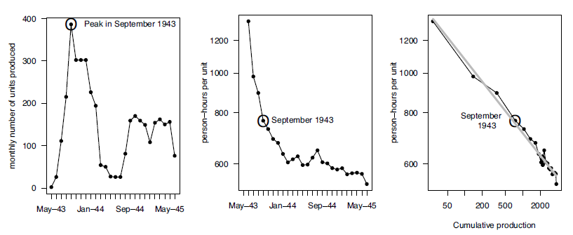
The massive build-up in military production was then followed by a dramatic slowdown. This makes the time series for production far from exponential and alleviates the problem of multicollinearity. Figure 1 illustrates a good example. Production of Ford’s armored car, model M-20 GBK, began in May 1943 and increased to a peak of 400 units per month by September 1943; it dropped dramatically by spring 1944, rising later but never to the previous level. In contrast, costs came down more or less continuously, and a plot of the logarithm of cost against the logarithm of experience yields an approximately straight line. The key point here is that costs continued to drop even as production decreased, lending evidence to the importance of cumulative production (experience) rather than production itself as a key variable (Asher Reference Asher1956, p. 87).
PRODUCTION (NUMBER OF UNITS PER MONTHS), PERSON-HOURS PER UNIT AND EXPERIENCE CURVE, USING CUMULATIVE PRODUCTION (WITH LINEAR FIT) FOR FORD’S ARMORED CAR M-20 GBK
Source: Ford’s archives.

To take advantage of this unique demand shock, we have gathered novel and unprecedentedly large amounts of data on U.S. military production during the war: time series on labor productivity, a cross-sectional dataset of unit cost declines for more than 500 products, and aggregate data on indices of contract prices broken down into 10 different categories.
These three datasets differ in terms of the main variable available (labor productivity vs. unit cost), number of observations (complete time series or not), level of aggregation (from plant to War Department level), and type of product. However, in combination, they provide an unprecedentedly comprehensive picture of industrial military production during WWII. While earlier studies have focused exclusively on complex “big ticket” items like ships and planes, our data captures the full gamut of war production: from mature technologies like rifles for the infantry to brand new technologies like early radar. To date, documentation of this diversity of production has been scattered across primary and secondary sources. Bringing it together represents a major contribution to the economic historical literature about WWII. In fact, we find that the rates of unit cost reductions were in general much smaller than what one could have thought based on the well-known examples of labor productivity growth in airplanes. This is likely to be because nonlabor costs, such as capital, became more prevalent, but also because airplanes were an exceptional category.
To further bolster the value of this data, we have applied new corrections for estimating cumulative experience prior to the beginning of production observed in our data. Generally, earlier studies have simply applied a correction based on the assumption that production grows exponentially both within the observed sample and the period before observation starts. Because exponential growth would be a poor assumption in our case and because our datasets cover highly heterogenous products, we developed an alternative method of estimating prior experience, using historical statistics that are available at a coarse level to correct for prior experience at a finer-grained level.
Our results make it clear that costs depend on both experience and an exogenous time trend, in roughly equal amounts. Thus, experience does cause cost improvements, lending support to arguments that state-sponsored demand can be effective to accelerate the development of critical technologies. Nonetheless, even in a historical moment of enormous government investment, some ultimate causes of declining costs are better proxied by the passage of time than by the growth of experience.
Unfortunately, our data does not allow us to evaluate deeper channels of causality. For instance, higher productivity that follows a rise in experience can be due to direct learning-by-doing or to any productivity-enhancing factor that tends to scale with experience, such as R&D. We refrain from commenting on these specific channels, and simply conclude that endogenous effects (as captured by experience at producing a specific product) and exogenous effects (as captured by a time trend or time dummies) explain about as much of the average rate of cost decrease. As a result, a large demand shock is likely to accelerate declines in costs of production.
An important contribution to historical studies of WWII is that the relationship between experience and cost is very heterogeneous: while for some products, costs decline sharply if experience increases, other products are less sensitive to experience effects. As a result, we conclude that a policy stimulus is only likely to be effective for a particular product when there is a favorable historical relationship.
LITERATURE REVIEW
We provide a review that focuses on the points of overlap between the economics literature about experience curves and the economic historical literature about the massive WWII production effort.
There is large literature documenting the relation between increasing experience, defined as cumulative production, and decreasing costs. The literature has its roots in Wright’s study of the aircraft industry but has now gone far beyond that, with studies ranging in aggregation level from individual plants to total global output of individual products.Footnote 2 It is clear that growing experience is positively correlated with cost declines, but the relative importance of the different channels through which this happens is an unsettled debate.
The most common explanation is simply learning-by-doing: individual workers and managers learn while they are on the job, improve the manufacturing process and thereby lower costs (Newell and Rosenbloom Reference Newell, Rosenbloom and John1981; Heathcote, Brown, and Mewhort Reference Heathcote, Brown and Mewhort2000). Military products have played an important role in the development of the concept of learning-by-doing in economics. According to Hirsch (Reference Hirsch1956), much of the early impetus to study the evolution of costs came from the U.S. Air Force, which was interested in cost decreases in airplane production. Theodore Wright himself was head of U.S. aircraft production during WWII and is reputed to have used his own law to forecast aircraft production costs. The Air Force commissioned a number of reports, particularly from RAND in the late 1940s and 1950s. These early reports suggested strong learning-by-doing effects in aircraft production (Asher Reference Asher1956; Alchian Reference Alchian1963). Using WWII U.S. shipbuilding data on the well-known Liberty Ships, Rapping (Reference Rapping1965) attributed the large decrease in person-hoursFootnote 3 per unit to organizational and individual learning from production experience.
However, since the publication of these studies in the mid-twentieth century, scholars have extended the simple learning-by-doing interpretation, focusing on capital intensity, quality of management, knowledge spillovers, and R&D.
A higher capital intensity is a particularly important driver of the reduction in labor needed per unit of production (Scott-Kemmis and Bell Reference Scott-Kemmis and Bell2010; David 1974). Thompson (Reference Thompson2001) collected better data on capital intensity in Liberty ships production, and found that learning-by-doing was largely overestimated, with labor productivity improving mostly thanks to higher capital stock. Mishina (Reference Mishina, Naomi, Daniel and Temin1999) studied the Boeing Seattle plant producing the B-17 Flying Fortress aircraft in detail and was able to control for capital intensity. He found that productivity stopped growing when production was scaled down, and he rejected cumulative production as a source of cost reduction. This is a finding that does not generalize in our dataset. Bahk and Gort (Reference Bahk and Gort1993) worked with plant-level data, measuring experience as cumulative production but adding a variable for capital vintages. One of their conclusions is that when the capital vintages variable is included, the effect of calendar time disappears—or even reverses—suggesting that “industry-wide” learning is actually capital embodied.
Looking at the production of ships during WWII, Searle (Reference Searle1945) found that the rates of cost reduction varied from one yard to another more than they did between different types of vessels within a given yard. This lends support to the idea that the quality of management within an organization has a significant effect on the cost of production, as Argote and Epple (Reference Argote and Epple1990) have argued. In a classic paper about the cotton spinning industry, Lazonick and Brush (Reference Lazonick and Brush1985) found evidence that management-worker relations impacted work intensity and productivity improvements.
Another well-studied source of cost improvement is experienced in the production of another model or by another firm. Thornton and Thompson (Reference Thompson2001) extended Thompson’s (2001) dataset with 57 different types of ships and studied a variety of experience spillovers, both between and across yards. They found that such spillovers could be quite important, though this is sensitive to the indicator used. Intergenerational externalities (between different generations of a product) have been identified by Irwin and Klenow (Reference Irwin and Klenow1994) and by Benkard (Reference Benkard2000). Irwin and Klenow (Reference Irwin and Klenow1994) also found strong international interfirm externalities in their study focused on the DRAM industry. Levitt, List, and Syverson (Reference Levitt, List and Syverson2013) estimated the effects of experience on labor productivity and defect rates in an automotive plant and documented in exceptional detail how learning by the workers of one shift was transmitted to workers of another shift.
More recent studies have focused on the effects of R&D on cost reduction. Sinclair, Klepper, and Cohen (Reference Sinclair, Klepper and Cohen2000) studied detailed product-level learning curves in the chemical industry, and found that the products for which there was the tightest connection between cost improvement and production experience were also those for which specific (process) R&D projects had been developed. They argue that because cumulative production conditions future returns to R&D, often cumulative production will be associated with R&D and thus to cost decrease. Funk and Magee (Reference Funk and Magee2015) have focused on the pre-commercial period of production. They showed that significant pre-commercial technological progress occurs before large-scale production experience occurs. Looking at firm-level, nonquality-adjusted unit costs in India, Dosi, Grazzi, and Mathew (Reference Dosi, Grazzi and Mathew2017) found that R&D-intensive sectors tended to exhibit a “negative” learning rate, pointing toward R&D as a source of quality improvement, leading to higher costs rather than cost savings. Another explanation for heterogeneous learning rates is design complexity: if engineers perform improvements by trial-and-error on parts of a more complex entity, more complex designs require more coordinated improvement, which is less likely (McNerney et al. 2011).
Despite detailed datasets and attempts at uncovering sophisticated channels that affect productivity, many studies tend to suffer from a more basic issue: because experience is a cumulative variable and it tends to grow exponentially, the inclusion of a time trend to correct for omitted variables results in serious multicollinearity that prevents precise estimation of relative effects.
Studies where including a time trend led to unstable results include Papineau (Reference Papineau2006), Söderholm and Sundqvist (Reference Söderholm and Sundqvist2007), and landmark papers in the experience curve literature, such as Benkard (Reference Benkard2000) and Bahk and Gort (Reference Bahk and Gort1993). The Liberty ships studies face the same issue. Thompson (Reference Thompson2001) does not control for a time trend, and Thornton and Thompson (Reference Thompson2001) do include a time trend but find that it has “the wrong sign.” In their regressions of defect rates on experience in an automotive plant, Levitt, List, and Syverson (Reference Levitt, List and Syverson2013) report opposite signs for the time trend and experience when using a small dataset (weekly data), but not with a larger (daily) dataset. This may be expected, as more data points compensate for the collinearity between the regressors.
A more complex issue is causality. While one approach has been to use instrumental variables (Benkard Reference Benkard2000; Söderholm and Sundqvist Reference Söderholm and Sundqvist2007, Witajewski-Baltvilks, Verdolini, and Tavoni Reference Witajewski-Baltvilks, Verdolini and Tavoni2015), we instead choose to exploit a classic natural experiment: military production during WWII, a setting in which we can gather comprehensive evidence, demand is exogenous, and the time trajectory of production is far from exponential, solving basic issues of causality and multicollinearity. However, it remains beyond the scope of this paper to settle the debates on which of the many channels of productivity improvement are most important. As noted by Levitt, List, and Syverson (Reference Levitt, List and Syverson2013), the relationship between productivity and cumulative production may be incidental to a deeper causal mechanism, involving direct accumulation of knowledge at the firm level, and possibly other sources of increasing efficiency when considering sector or product level experience curves.Footnote 4 Our contribution is to focus on one simple problem—the relative contribution of exogenous and endogenous factors to productivity growth—and to address it with as much data as possible. We stick to a simple distinction between causal factors that are well proxied by product-specific accumulated experience, and causal factors that are independent of this but are the same across all products.
A UNIQUE HISTORICAL CONTEXT
The demand shock to military equipment production in the United States caused by WWII was enormous. President Roosevelt made this clear in his “Arsenal of Democracy” fireside chat on 29 December 1940, when he said,
I want to make it clear that it is the purpose of the nation to build now with all possible speed every machine, every arsenal, every factory that we need to manufacture our defense material (Roosevelt Reference Roosevelt1940).
When war broke out in Europe in September 1939, the U.S. Army had only 189,839 men and women (Herman Reference Herman2012). By the time of Pearl Harbor, it was more than 1.4 million men and women strong (The National WWII Museum 2015). Defense spending increased almost 30 times between 1940 and 1942. The United States supplied the Soviet Union and the United Kingdom with war materiel, particularly the United Kingdom after enacting the Lend-Lease policy Act in 1941. Qualitative evidence suggests that the period between the autumn of 1939 and the American entry into WWII was important for preparing the United States for war production. This ramp-up continued throughout the war. Between 1943 and the end of the war in 1945, the U.S. government spent four times as much money on war production as it had spent in 1942 (Koistinen Reference Koistinen2004).
However, these huge expenditures were not allocated to clear and consistent munitions orders. Instead, “munitions orders kept changing …as the project size of the American Armed Forces increased as the American military strategy evolved” (Carew Reference Carew2009). As documented in the Army’s own history of its role in economic mobilization in WWII, “automatic supply gave way in large measure to supply on the basis of specific requisitions from theatre commanders. This permitted procurement and issue of supplies more closely tailored to specific theatre needs as indicated by operation experience and changes in strategic plans” (Smith Reference Smith1959, p. 173).
Support for battlefield victory at all costs continued throughout the war. From the highest office to the internal operations of the responsible bureaucracies for military production and procurement, the priority was battlefield victory—rather than cost savings. In August 1943, the War Department Procurement Review Board was appointed to evaluate the composition, essentiality, and balance of procurement programs. It noted that “a war cannot be run like an industry; the criterion is not low costs but victory” (Smith Reference Smith1959, p. 159). In 1940, the War Production Board set forth 12 criteria for the placement of contracts, including speed of delivery, quality, and price. In contrast, the War Production Board statement of March 1942 contained three ordered criteria: speed of delivery; conserving of superior facilities for the most difficult items of production; and placement of contracts with firms needing the least amount of additional machinery and equipment (Smith Reference Smith1959, p. 263). This strongly suggests that companies were operating at maximum capacity and that using available capacity, rather than finding the cheapest supplier, was the key driver of procurement decisions. Price and cost efficiency criteria were reintroduced explicitly in late 1942 and 1943 but were never leading criteria.
The procedures for managing costs and awarding contracts evolved during the course of the war. For products whose structure and costs of production were well known, Fixed-Price contracts were the government’s first preference. In situations where firms were creating new products with unknown costs the government instead used Cost-Plus-a-Fixed-Fee (CPFF) contracts. In 1941 contracts began to include renegotiation clauses, which meant that at the conclusion of the contract a renegotiation would take place between firms and the government to assess actual costs (Smith Reference Smith1959). This practice was codified with the passage of the 1942 Renegotiation Act and linked legislation that made renegotiation a condition of all contracts or subcontracts greater than $100,000 (later revised up to $500,000). Producers were allowed to maintain a fluidly defined “fair profit” in renegotiation, which was typically between 5 and 13 percent. Renegotiation ultimately saved the government approximately $3 billion on 118,000 contracts (Koistinen Reference Koistinen2004). Furthermore, it provided an incentive to conduct the detailed cost accounting that generated the data central to this paper.
While this was the general structure of contracting, procurement generally became more complex as a function of the complexity, novelty, and expense of the product being procured. Our comprehensive data captures this range of experiences because it expands the sample of products studied beyond just a handful of complex products. A clear example of this is the well-documented contracting process for aircraft during WWII (Holley Reference Holley1964). For the government to reach deals with aircraft and airplane engine makers, there was a longer initial negotiation process and then a more comprehensive renegotiation than for less complex products. This allowed both parties to adjust agreed-upon terms as they learned more about production costs and predicted efficiencies in production—including those predicted by Wright’s law, which the government frequently used as an analytical tool in negotiation. In short, while there are commonalities across contracting for WWII, the process was not completely homogenous.
The universal inclusion of renegotiation clauses meant that contractors had limited incentives to decrease their costs of production, as they would only be compensated for final demonstrated costs. As has been already noted in the WWII learning literature (Bajari and Tadelis Reference Bajari and Tadelis2001), there is little incentive in a cost-plus contract to supply a product more cost-efficiently. That said, while the contracts themselves do not provide clear incentives for learning, the process of defense procurement does: a high-performing supplier could expect more orders from the government (Rogerson Reference Rogerson1994). This possibility of repeat contracts as an incentive for learning and driving costs down may limit our exogeneity argument—at least when seen at the firm-level. However, the combination of the vast scale of the war effort and the intense pressure to ramp production up quickly made controlling costs difficult and required manufacturers to operate at near maximum capacity. The vast scale of the effort was so large that the majority of manufacturing firms in the United States were engaged in war-related production, and, together with the accelerated contracting process, this limited the ability of the government to select the most efficient producers when awarding contracts.
At the sectoral level, an argument can be made that cost played a role in determining which equipment was produced. The U.S. government intended to produce the deadliest weaponry at the lowest cost,Footnote 5 so that the relative demand for products that were substitutes was not independent of price. For instance, to the extent that two types of planes could be substituted for one another, the cheaper one may have been favored. Nonetheless, this was balanced by the fact that military strategy requires a diverse portfolio of different types of military equipment deployed in unison. The war could not be won by planes alone, but also required naval vessels, tanks, troop carriers, bullets, and a host of different types of equipment. Even within a category such as planes, military history suggests product complementarity rather than substitutability, for instance between bombers and fighters.Footnote 6 In any case, our data is quite comprehensive, covering individual products (which may have been substitutes) and aggregates (that are clearly not substitutes).
While we focus on the American context of wartime production and the effects of this large demand stimulus, several papers suggest there may be other international data available for consideration and comparison. For example, Budrass, Scherner, and Streb (Reference Budrass, Scherner and Streb2010) study learning-by-doing and fixed-price contracts for aircraft in Germany during the war, while Okazaki (Reference Okazaki2011) focuses on Japanese airframe production. However, these papers—like earlier work on U.S. war production—focus on one narrow type of wartime production, in this case, aircraft. Furthermore, while the United States was able to produce for the war with relatively limited interruption from battles on the home front, the same was not true for Axis powers or even European Allies. As Tooze (Reference Tooze2005) carefully demonstrates, German production was severely compromised by the Allied siege as the war progressed. Working far from the frontlines, the United States was able to ramp up production in an exceptional way and, as our data indicate, maintain extremely detailed records about wartime production.
DATA
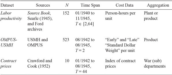
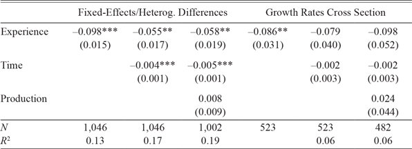
Another key specific advantage of the historical context is that because many products were bought by the government, prices were recorded at a fairly detailed level and are now part of the public record.Footnote 7 Using a number of different sources, we created three datasets, as summarized in Table 1. The datasets are ordered from the most fine-grained to the most aggregated. The first dataset comprises time series of production and labor productivity for 152 types of aircraft (or plant-aircraft pairs), ships, and motor vehicles, 23 of which have never been published before. The second dataset consists of time series of production for 523 products from all categories of war materiel, paired with “early” and “late” unit costs. This dataset is new. The third dataset comprises time series for indices of contract prices for several branches of the War Department. While this last dataset was easy to collect, we are not aware of any study that has matched the relevant tables to construct experience curves from it.
SUMMARY OF THE THREE DATASETS

Notes: N is the number of time series and T is the number of observations in each time series. Time span refers to cost data. In each dataset, we have production data starting in January or July 1940.
Source: The authors.
We now describe each dataset more precisely, leaving the full details of data collection to Online Appendix A.
Labor productivity in Aircraft, Ships, and Motor Vehicles
Our first dataset, which we will refer to as Labor productivity, includes time series of labor productivity from three different sources (see Table 2). The first source is the well-known time series of labor productivity for ships, extracted from Searle (Reference Searle1945). It has been already widely extended and analyzed in Rapping (Reference Rapping1965), Thompson (Reference Thompson2001, 2007), and Argote, Beckman, and Epple (Reference Argote, Beckman and Epple1990).
SOURCES OF THE LABOR PRODUCTIVITY DATA

Source: The authors.
The second source is an extension of the data used in the study of aircraft by Alchian (Reference Alchian1963), extracted from the source quoted in his paper, referred to as the Source Book (Army Air Forces 1947). It contains data on plant-product pairs, so the same plane in different plants is a separate time series, and so are different planes within the same plant.
The third source is entirely original. We have collected a novel set of time series from Ford’s archive. This covers 23 products, mostly motor vehicles. Online Appendix A.1 further discusses data collection and transcription issues for each of these three sources.
Total Unit Costs at the Product Level
Our second dataset, which we will refer to as OMPUS-USMH or OMPUS for short, was created by combining two archival publications. The first publication, Official Munitions Production of the United States, by Months, July 1, 1940–August 31, 1945 (OMPUS) Handbook (Civilian Production Administration 1947), provides information about the monthly output of particular categories of munitions and specific products. The second publication is the United States Munitions Handbook (USMH), which provides the costs of production, in terms of “Standard Dollar Weights” at two moments—one at the beginning of the war and one towards the end—for many of the products recorded in the OMPUS. While the OMPUS is available online, the formerly classified USMH was located in the National Archives by one of us (D.G.).
Matching OMPUS to the USMH was relatively easy because each product listed in the USMH includes the page and column to which it should be matched in the OMPUS. One of the nice features of these data is that they are nearly comprehensive. The OMPUS publication was intended to record the “munitions figures of all of the procurement services” (our emphasis), and while the USMH does not report cost values for the majority of products, the coverage appears reasonably representative.
The main issue we had with the dataset concerned the dates at which the costs were recorded; the dates in the USMH are the same for every product category, but some products started production after the “early” date or ended production before the “late” date—in this case, we assumed, guided by the USMH explanatory notes, that the early/late dates corresponded to the start/end of production. Online Appendix A.2 provides a more detailed discussion of our interpretation of early and late costs and Standard Dollar Weights.
While the OMPUS provides production data, it does not provide data on experience, that is, cumulative production since the first unit. It is impossible to know what the previous manufacturing experience was for each product listed in the OMPUS. While other studies of experience curves have not corrected for prior experience or have applied a correction based on the assumption of exponential growth, we opted for an approach that corrects at the level of semi-aggregated categories, for which we could obtain rough estimates or introduce one ourselves. For each product i, we estimated prior experience as a proportion of total war production experience. More precisely, we estimated initial experience as a category-specific factor ζ i times the total amount of known production of product i during the war
 ${\mathop \sum _{\tau = 1}^T {Q_{i,\tau}}}$
. Denoting experience Z i,t, we have
 $$\begin{equation}{{Z_{i,t}} = {\zeta _i}\sum\limits_{\tau = 1}^T {{Q_{i,\tau }}} + \sum\limits_{\tau = 1}^t {{Q_{i,\tau }}} ,\;} \\ \end{equation}$$
where T is the total number of months from January 1940 to August 1945. The first term represents estimated initial experience, and the second term is the usual experience computed as observed cumulative production up to time t.
Because these products are too detailed, we attempted to estimate the factors ζ i at a more aggregated level, using the 81 most detailed levels of the table of contents of the OMPUS. The ζ i and the extensive discussion of how we estimated them are provided in Online Appendix B. To give one example, consider fighter aircraft. We have 12 models of fighters in the USMH-OMPUS data, and we do not know the initial experience of each model. However, from other sources, we were able to estimate that around 300,000 planes were produced during WWII, and a total of 60,000 were produced at any time before the war. Therefore, we applied a value of ζ ≈ 60,000/300,000 = 0.20 to all aircraft models. For example, 680 units of the P–61 Black Widow model (OMPUS ref. 15/3) were produced during the war, so we constructed the experience variable as if 0.20 × 680 ≈ 136 models had been produced before.
Contract prices at the War Department Level
Our last dataset, which we will refer to as Contracts, contains contract price indices and is taken from the statistics on procurement in Crawford and Cook (1952). This data allows us to construct experience curves for the period January 1942–August 1945 at several different levels of aggregation. The data is for the eight different branches of the War Department. The highest level of aggregation is the entire War Department. It is then subdivided into the Air Forces (AAF) and the Service Forces (ASF). The latter is then subdivided into seven technical services, which “were the operating agencies of the War Department in all its supply activities” (Smith Reference Smith1959, p. 114).
The data on production, while expressed in millions of dollars, can be taken as indicative of production volume because it has been generated from a large sample of physical quantities, evaluated at 1945 prices rather than at the prices in force during each month. The indices of contract price changes were computed from price changes to contracts for individual products, representing about half of the total value of War procurement. As for the OMPUS data, we estimated prior experience as a category-specific factor times the total level of wartime production. The detailed justification for the correction factors applied to this data is also given in Online Appendix B.
EMPIRICAL FRAMEWORK
Our objective is to estimate the effect of experience on cost. As discussed previously, simply regressing cost on experience, as is done in learning curve studies, suffers from several related issues, all of which are absent or limited in the context of WWII military production.
To restate the issues, because demand is generally elastic, the relationship between price (or cost) and production (or experience) embodies both demand elasticity and the causal effect of experience on cost. However, while demand relates price/cost and production, the effect of experience is between cost and cumulative production. It is common (outside of WWII) that production grows exponentially, so cumulative production grows exponentially too, at the same rate. Because of this, if we use production and cumulative production interchangeably, we can think of the issue as a problem of simultaneity between cost/price and production/experience (Nordhaus Reference Nordhaus2014), even though the mechanisms are in principle from experience to cost and from price to production.
Second, it is easy to argue that cost reductions cannot possibly come only from the growth of product-specific experience, whatever these proxies are.Footnote 8 The simplest possible way to acknowledge omitted variables is simply to allow for an exogenous exponential time trend, to capture overall economy-wide trends. However, as discussed in the previous paragraph, experience often grows exponentially and in a smooth manner (Lafond et al. Reference Lafond, Aimee Gotway Bailey, Dylan Rebois, McSharry and Doyne Farmer2018), making it hard to distinguish the effect of experience from the effect of an “exogenous” exponential time trend. Technically speaking, this is just an issue of imperfect multicollinearity. In the specifications in first-differences, where the exogenous time trend is simply the intercept of the regression, this is just an issue of limited variance of the regressor. While in principle this does not bias the coefficients, including both experience and a time trend usually makes standard errors extremely large and gives unstable results, as discussed in the Literature Review section. It is therefore a serious issue.
Nordhaus’s Model
Nordhaus (Reference Nordhaus2014) introduced a very simple model that illuminates the issues and helps clarify why demand exogeneity makes the identification of the effect of experience on costs possible.
Let Q t denote production at time t and let Z t denote cumulative production. Assume the unit cost function
 ${c_t}$
depends on both experience Z t and an exogenous time trend, with the functional form
 $$\begin{equation}{{c_t} = {c_0}Z_t^{ - b}{e^{ - at}}.}\end{equation}$$
The parameters a and b are expected to be positive since we generally observe technological progress. Assume that production is equal to demand and price is equal to unit cost.Footnote 9 Furthermore, assume that demand has constant elasticity ε > 0 and that there is an exogenous and growing demand e dt . This givesFootnote 10
 $$\begin{equation}{{Q_{t}} = {D_{t}} = \mathop {{D_0}{c_t^{ - \varepsilon}}} {e^{ - dt}}\;}.\end{equation}$$
By letting Δ represent the time difference operator Δx = x t – x t–1, Equations (2) and (3) can be written as
 $$\begin{equation}{\Delta {\rm{log}}c = - a - b\Delta {\rm{log}}Z}\end{equation}$$
and
 $$\begin{equation}{\Delta {\rm{log}}Q = - \varepsilon\Delta {\rm{log}c} +d.\ }\end{equation}$$
Now, suppose that production grows exponentially. Then experience also grows exponentially at the same rate, that is
 $$\begin{equation}{\Delta {\rm{log}}Q \approx \Delta {\rm{log}}Z.}\end{equation}$$
Using this in Equation (5), the solution of the system of Equations (4) and (5) is
 $${\Delta \log{c} = \frac{{ - a - bd}}{{1 - b\varepsilon}}},$$
 $$\begin{equation}{\Delta \log Z = \Delta \log Q = \frac{{a\varepsilon + d}}{{1 - b\varepsilon }}.}\\ \end{equation}$$
Nordhaus (Reference Nordhaus2014)’s critique is that experience curve studies typically assume that the logarithm of experience is the single explanatory factor for the logarithm of costs. In other words, they assume that
 $$\begin{equation}{\Delta {\rm{log}}c = \beta \Delta {\rm{log}}Z,}\end{equation}$$
and perform a regression of the logarithm of costs against the logarithm of experience in order to measure the empirical parameter β. Inserting Equations (6) and (7) into Equation (8), we can write the parameter β as the ratio
 $$\beta \begin{equation}{ = \frac{{\Delta \log c}}{{\Delta \log Z}} = \frac{{ - a - bd}}{{a\varepsilon + d}}.} \\\end{equation}$$
It is clear that in general, the empirically estimated parameter β not only depends on the experience parameter –b, but it also depends on the exponential trend parameter a for costs, the exponential trend parameter d for exogenous demand growth, and the demand elasticity ε. The estimated β can be interpreted as being purely the effect of experience only when there is no exogenous time trend. In other words, if a = 0 then β = –b.
Let us now consider the case in which demand is completely exogenous (ε = 0), but for simplicity still growing exponentially. In this case Equations (6) and (7) become
 $$\begin{equation}{\Delta {\rm{log}}c = - a - bd,}\end{equation}$$
and
 $$\begin{equation}{\Delta {\rm{log}}Z \approx \Delta {\rm{log}}Q = d,}\end{equation}$$
so that putting Equation (11) into Equation (10) gives
 $$\begin{equation}{\Delta {\rm{log}}c = - a - b\Delta {\rm{log}}Z,}\end{equation}$$
which is the same as Equation (4). If demand is completely exogenous, we can estimate the supply equation directly.Footnote 11 A simple first-difference regression model for the logarithm of cost against the logarithm of experience with an additive constant is able to separate the effects of the exogenous trend parameter a and the “learning” parameter b.
While illustrative of the reverse causality issue, this model is not stochastic and all variables grow exponentially, so it cannot do justice to the other important issue, multicollinearity. If production grows exponentially with fluctuations, since computing experience from production involves integrating and therefore smoothing, Z will increase exponentially but with much lower fluctuations, so the term ΔlogZ t will be approximately equal to the constant d, for all t. Footnote 12
Fortunately, we will find empirically that during WWII, demand exogeneity led to production patterns that were not exponential, making the correlations between the regressors (time, production, and experience) much lower than in other studies using recent data.
Main Specification
It is customary in the literature to motivate the main specification for learning curve regressions by starting from the standard Cobb-Douglas production function. This does not assume exponentially increasing production, it allows for economies of scale, and it can be used with data on labor productivity.Footnote 13 With constant technical parameters and a time-varying Hicks-neutral productivity factor A t that depends on experience and an exogenous time trend, as in Rapping (Reference Rapping1965), we have
 $$\begin{equation}{{Q_t}{ = A_t}K_t^{{\theta _k}}L_t^{{\theta _l}},}\end{equation}$$
 $$\begin{equation}{{A_t} = Z_t^b{e^{at}},}\end{equation}$$
where K t and L t are capital and labor in period t and θ k and θ l are constants, with an additional term for an exponential exogenous productivity improvement as in Nordhaus (Reference Nordhaus2014).
If firms minimize their total cost subject to the constraint of fixed exogenous demand
 $${Q_t} = {\bar{Q_t}}$$
, and factor prices are constant, the optimal labor demand per unit of production can be written
 $${\text{log}}\frac{{L_t^{\text{*}}}}{{{{\bar Q}_t}}} \equiv {\text{log}}\;{l_t} = {B_L} - \left( {\frac{a}{s}} \right)t - \left( {\frac{b}{s}} \right){\text{log}}\;{Z_t} + \left( {\frac{1}{s} - 1} \right){\text{log}}{\mkern 1mu}{\bar{Q_t}} ,$$
where B L is a constant and where s = θ k + θ l represents economies of scale. Since we have data on the unit labor requirements
 ${l_t} = L_t^{\rm{*}}/{\bar{Q_t}}$
in our Labor productivity dataset, we can estimate this equation. In the two other datasets, we have data on total unit costs
 ${c_t} = {C_t}/\bar {{Q_t}}$
. Inserting optimal factor requirements in the total cost function
 ${C_t} = wL_t^{{*}} + rK_t^{{*}}$
gives
 $$\begin{equation}{{\rm{log}}\frac{{{C_t}}}{{{{\bar Q}_t}}} \equiv {\rm{log}}\;{c_t} = {B_C} - \left( {\frac{a}{s}} \right)t - \left( {\frac{b}{s}} \right){\rm{log}}\;{Z_t} + \left( {\frac{1}{s} - 1} \right){\rm{log}}\bar {\;{Q_t}},}\end{equation}$$
where B C is another constant. Apart from the constants, the Equations (14) and (15) are the same. They become exactly the same if we estimate a model in first differences, that is
 $$\begin{equation}{\Delta {\rm{log\;}}c = \Delta {\rm{log\;}}l = - \left( {\frac{a}{s}} \right) - \left( {\frac{b}{s}} \right){\rm{log}}\;{Z_t} + \left( {\frac{1}{s} - 1} \right){\rm{log}}\;{{\bar Q}_t}.}\end{equation}$$
Our favored specification is to estimate Equation (16) in a pooled panel. However, each dataset presents specific patterns of missing data and thus different opportunities for robustness checks and alternative specifications—typically fixed effects for the levels (Equations (14) and (15)) and separate regressions for each time series. Thus, we present our detailed econometric specifications separately for each dataset.
EMPIRICAL RESULTS
We now present results from performing regressions on the three data sets here.Footnote 14 A point of prior optimism comes from examining the correlations between the independent variables. As shown in Table 6, they range from about 50 to 90 percent. Although this might seem high, they should be compared with systematically higher correlations in other contexts, such as the chemical industry numbers reported by Lieberman (Reference Lieberman1984), which are all greater than 90 percent.
Labor productivity in Aircraft, Ships, and Motor Vehicles
A typical model specification (Lieberman Reference Lieberman1984) for analyzing a panel of experience curve time series is the fixed effects model
 $$\begin{equation}{{\rm{log\;}}{l_{it}} = {\kappa _i} + \alpha \;t + \beta \;{\rm{log\;}}{Z_{it}} + \gamma \;{\rm{log}}\;{Q_{it}} + {\eta _{it}}.}\end{equation}$$
Comparing to Equation (14), κ i = B L, α = –a/s, β = –b/s and γ = 1/s –1. The results of this model applied to the Labor productivity dataset are reportedFootnote 15 in Table 3. Including only experience, we find that β ≈ –0.33, which implies a drop of cost of 20 percent for each doubling of experience. This number coincides with the original observation by Wright and is seen in many other studies of products such as airplanes. The estimated coefficient for the exogenous time trend is not very statistically significant, but its value is relatively high; given that the data is monthly, a negative coefficient of 0.004–0.006 implies an annual rate of exogenous technological progress of about 5 to 7 percent. Finally, including production indicates very mild and not very significant economies of scale. Throughout the paper, we will find no convincing evidence of non-constant returns to scale.Footnote 16
PANEL REGRESSION RESULTS FOR LABOR PRODUCTIVITY

Source: The authors.
A typical feature of experience curves regressions is that they have highly autocorrelated residuals (Thompson 2012). We ran the test of Wooldridge (Reference Wooldridge2002) for AR(1) residuals in short panels and found in all three cases very strong evidence against the null of no first-order autocorrelation. This suggests estimating a model with autocorrelated disturbances, or a model with lags of the dependent variable, which we do in Online Appendix D.1. But since we are not interested in the intercepts, and since from a theoretical point of view, we expect that it is the change in experience that induces a change in cost, we favor a first-differences specification,Footnote 17 that is
 $$\begin{equation}{\Delta {\rm{log}}\;{l_{it}} = \alpha + \beta \;\Delta {\rm{log}}\;{Z_{it}} + \gamma \;\Delta {\rm{log\;}}{Q_{it}} + {\eta _{it}}.}\end{equation}$$
The role of experience is fairly consistent with the fixed effects regression, but it indicates a larger role in the time trend. The coefficient β now ranges from –0.25 when only experience is included to –0.20 when all independent variables are included and remains solidly statistically significant. However, the coefficient α for the exogenous time trend now has a value of –0.024 when all variables are included, corresponding to a much larger annual improvement rate of about 29 percent, and is now strongly statistically significant. As we will discuss in the Discussion section, this represents a third of the rate of cost decrease, with the other two-thirds accounted for by experience. When including production, the coefficient γ is now very small and statistically insignificant.
Finally, we present the results of independent regressions for each individual product or plant, removing all time series with less than 10 available cost values (so 118 of 152 time series remain). Since the coefficient for production is so small in the aggregate regression, we exclude the production variable here in the interest of parsimony. The equation estimated is
 $$\begin{equation}{\Delta {\rm{log}}\;{l_{it}} = {\alpha _i} + {\beta _{i\;}}\Delta {\rm{log}}\;{Z_{it}} + {\eta _{it}}.}\end{equation}$$
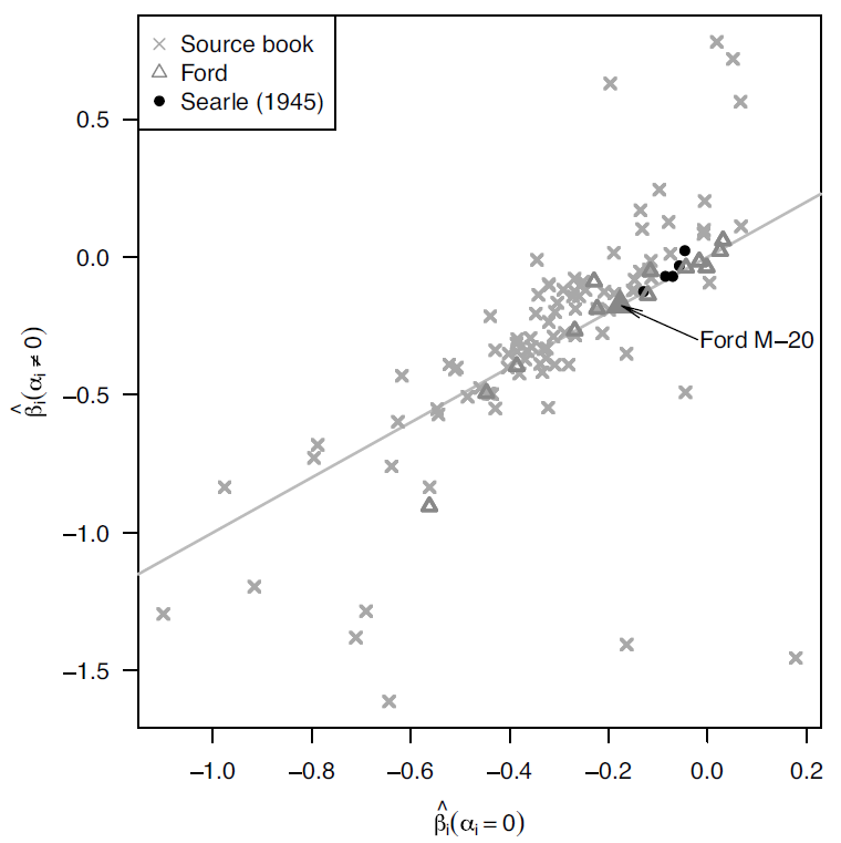
Figure 2 compares the estimated coefficient
 $$\hat \beta $$
for the regression Equation (19) when the exogenous time trend is included to the case where it is not, that is, we restrict α i = 0 and Equation (19) becomes a regression through the origin. We observe a great deal of heterogeneity in experience rates, but the results are broadly consistent with the aggregate regression. The variation is a mixture of intrinsic differences in real progress rates and statistical fluctuations due to the fact that the individual regressions are based on short time series (we have also checked that there is no correlation between the estimated slope parameter and the number of available observations). With some exceptions, most of the data is clustered along the identity line, demonstrating that the coefficient estimated for experience is not overly sensitive to the restriction α = 0. This stands in sharp contrast with the results reported by Nordhaus (Reference Nordhaus2014). Figure 2 in Nordhaus (Reference Nordhaus2014), which is analogous to our Figure 2, shows coefficients that are often extremely far from the “reasonable” range β ∈ (0,–0.5), and which change by more than an order of magnitude when a time trend is included. We believe that the main difference is that in his data, many of the production time series (and thus experience time series) are close to following an exponential trend, creating extreme problems of multicollinearity.
COEFFICIENT β i FOR EXPERIENCE WHEN THE TIME TREND IS INCLUDED, PLOTTED AGAINST THE SAME COEFFICIENT WHEN THE TIME TREND IS NOT INCLUDED, USING EQUATION (19)
Notes: The grey line is the identity. Three values of β i, which were greater than two in absolute value have been excluded. The Ford Armored Car discussed in the introduction (Figure 1) is shown as a slightly larger solid triangle.
Source: Own estimates based on the Labour Productivity dataset.

In summary, for the Labor productivity dataset, we observe a strong and clear relationship between declining labor costs and experience, with exponents β ≈ –0.2. We also show a significant role for the exogenous time trend, whose overall effect is comparable to that of experience (the Discussion section will provide an estimate of the relative importance of each variable for all the datasets).
OMPUS-USMH: Unit Costs at the Product Level
We now turn to the OMPUS dataset, which gives total unit costs instead of labor productivity and contains a more complete sampling of military products. A limitation is that we observe the cost for each product on only two different dates, and these dates differ across products. Nonetheless, because we assume that the parameters are the same for all products, we can exploit cross-sectional heterogeneity. We do this in two ways.
First, we are still able to estimate a fixed-effects model, but we also interpret it as a “differences” estimator. As is well-known, when T = 2, the first-differences and the fixed-effects estimators are the same. Online Appendix C shows that this result holds when the differences are heterogenous, in the sense that the span of time between the two observations is different from one product to another. We perform inference and report R 2 from the fixed-effects estimation.
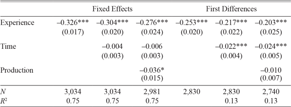
Table 4 shows the results of the regression, first including only experience and then including an additional time trend and production. The coefficients for experience are statistically significant but are smaller than for the Labor productivity time series, ranging from –10 percent when the other variables are not included to about –5.5 percent when time is included. The coefficients for the exogenous time trend are also significant, and about 0.4 percent per month or 5 percent per year (about 60 percent of the rate of cost decreases). As before, the coefficient for production is small and statistically insignificant.
PANEL REGRESSION RESULTS FOR OMPUS-USMH

Source: The authors.
Second, since with two observations we can compute an average growth rate, we perform a cross-sectional regression of the growth rates (Columns (4)–(6); see Online Appendix C, Equation (25) for details). The results are similar, although with a sensibly higher coefficient for experience and lower statistical significance.
The upshot is that the results for the OMPUS-USMH dataset are broadly consistent with those of the Labor productivity dataset, albeit with smaller experience exponents.
Contract prices at the War Department Level
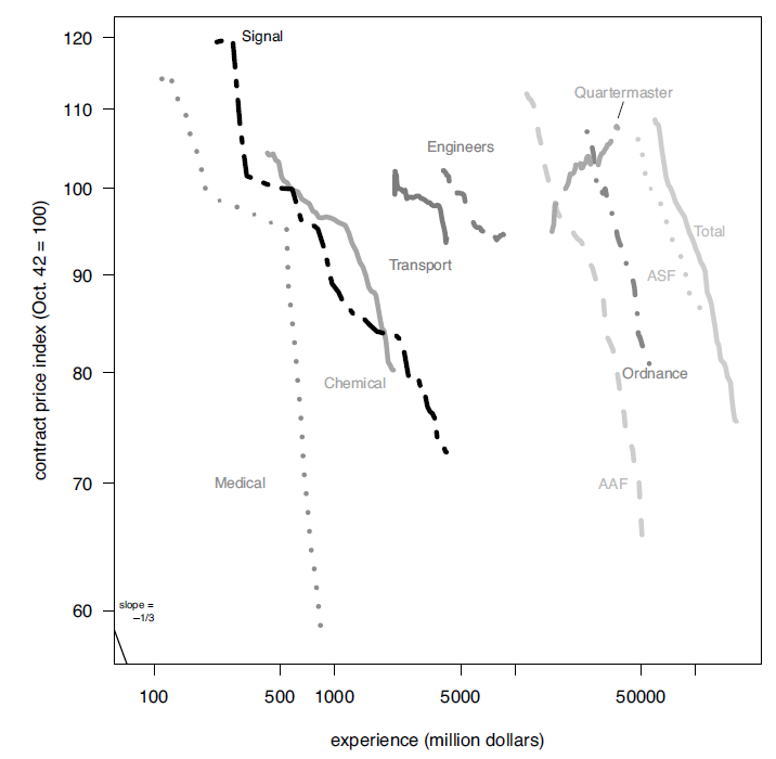
Figure 3 shows costs against experience in our last dataset on contract price indices at the War Department level. “Total” (on the right) represents the entire War Department, which is divided into Army Air Forces (AAF) and Army Service Forces (ASF); the latter is subdivided into the other seven services. Apart from Quartermaster, which saw its price increase over the period,Footnote 18 the other services have a relatively similar slope.
EXPERIENCE CURVES FOR THE WAR DEPARTMENTS AND COMPONENT AGENCIES
Source: Crawford and Cook (1952).

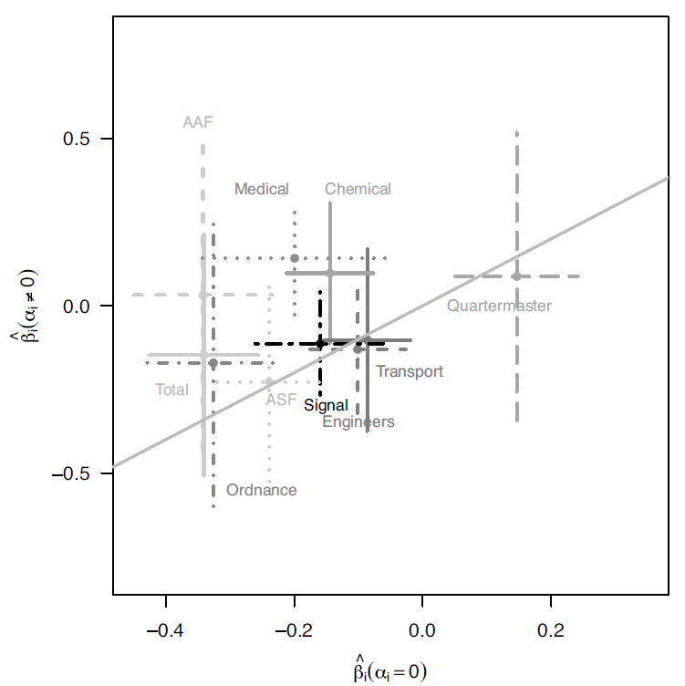
In Figure 4, we show the experience coefficient obtained from separate regressions for each individual time series, with and without the exogenous time trend. We make four observations that will be useful as a background to motivate the panel specification and understand its result.
ESTIMATED COEFFICIENT OF THE FIRST DIFFERENCE REGRESSION OF THE LOG OF CONTRACT PRICES ON THE LOG OF EXPERIENCE, INCLUDING OR EXCLUDING AN EXOGENOUS TIME TREND
Notes: The lines show plus or minus 2 HAC standard errors. The solid grey line is the identity.
Source: Authors’ estimates based on the Contract prices dataset.

First, in most cases, we see that standard errors are higher when the time trend is included, again reflecting the multicollinearity problem. Second, for some subservices (Ordnance, Signal, Transport, and Engineers), the coefficient is only slightly affected by the inclusion of the time trend, which in this case confirms that the lack of correlation allows us to pin down the relative effects of the exogenous trend and experience. However, for some other subservices (Medical, Chemical), the estimated coefficient changes so much that its sign flips. Third, when the time trend is included, all subservices have confidence intervals overlapping zero, indicating a lack of statistical significance. Fourth, the confidence intervals of all subservices largely overlap, suggesting that a panel regression assuming a unique slope could give sensible results.
PANEL REGRESSION RESULTS FOR CONTRACTS

Source: The authors.
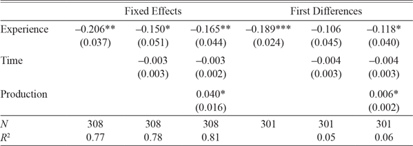
Because Quartermaster has such an obviously different slope in Figure 3 (on the top right), we remove it from the dataset and present panel regression results for seven time series (AAF and six subservices of ASF).
Table 5 shows the results. In line with previous estimates, we find an economically significant effect for both experience and the time trend, and a weak effect for production.Footnote 19
DISCUSSION
In this section, we take stock of the results obtained from the three datasets and briefly summarize our robustness checks.
Summary of the Results
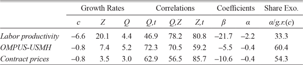
To provide an overview of our results, we have gathered some key statistics in Table 6. The first three columns show the average growth rates of the variables, computed as the average one period change in their logarithm, pooling all observations for which both Δlogc and ΔlogZ are available.Footnote 20 The next three columns show the Pearson correlations on pairwise complete observations between the “within” transformation of the regressors. The next two columns report the coefficients for the main regression specification, which includes experience (coefficient β) and time (coefficient α) and is estimated in first-differences (fixed-effects or equivalently “heterogenous differences” for the OMPUS, see Online Appendix C). The last column shows the ratio of α to the average growth rate of cost, which is the share of cost decrease accounted for by the exogenous trend.Footnote 21
DESCRIPTIVE STATISTICS AND MAIN RESULTS

Notes: All values are multiplied by 100. Growth rates are monthly. g.r.(c) is the growth rate of costs.
Source: The authors.
As is evident from the first column of the table, costs in the Labor productivity dataset, which are unit labor requirements, decline more than seven times faster than either of the two unit costs. One explanation is simply that improvement rates are heterogenous and the Labor productivity data comes overwhelmingly from the rapidly improving aircraft industry, while the other datasets on unit costs have a much wider and balanced coverage. Another explanation could be that capital deepening during the period improved labor productivity more than overall productivity.
The three columns giving correlations between the independent variables demonstrate that multicollinearity is a limited issue in our data. Although many of these correlations are high, they are still much lower than those reported in most previous studies (see, for instance, Lieberman Reference Lieberman1984, table 2).
The following two columns provide an overview of our regression results. In every case, both experience and the exogenous time trend play an important role. Given the larger rate at which costs decline in the Labor productivity dataset, it is not surprising that both effects are substantially larger in this dataset.
In the last column, we divide the exogenous trend rate α by the overall rate of cost decline (the figures in the first column of the table). This ratio is roughly a third for the Labor productivity dataset but 60 percent for the OMPUS-USMH and a half for the Contract prices datasets. Online Appendix D9 shows that while the estimated coefficients α and β are likely to be different across datasets (considering the standard errors associated with these estimates), the hypothesis that cost decreases are due to both endogenous and exogenous processes is relatively similar amount is much more defensible.
The overall conclusion is that we see a substantial effect of both experience and an exogenous time trend, in roughly equal proportions. This makes it clear that technological improvement is neither fully exogenous nor fully endogenous. Once we control for time and experience, the effect of monthly output is negligible. When multicollinearity is not as severe as in other settings, and enough data are pooled together, the estimates are relatively stable across specifications.
Robustness of the Results
We discuss the robustness of the results to changes in econometric methodology, assumptions about initial experience, and omitted variables. The details of the robustness checks, when possible, are in Online Appendix D.
Time series analysis (D.1)
Overall, we tend to find similar results to those reported in the text if we (a) include time fixed effects instead of an exponential trend, (b) replace experience by its lagged value, and (c) test for times series properties and estimate the models suggested by these tests.
Heterogenous coefficients (D.2)
We allowed for fixed effects in the first difference regression, thereby allowing for time trends to differ. This had no effect on the Labor productivity dataset, but for the Contracts data, the effect of experience disappears completely, although standard errors are large enough that we cannot reject a value such as the one estimated in the main text. Estimating Swamy’s (1970) or Pesaran and Smith’s (1995) heterogenous coefficient models gives the same outcome, with robust results for Labor productivity but not for Contracts.
Instrumenting by lagged values (D.3)
Our dependent variable is a total (either person-hours or cost) divided by output. Thus, output appears on both sides of the equation. We instrumented output and experience by their lagged value and found that this does not change the results.
Alternative assumptions on initial experience (D.4)
We re-estimated our models using different assumptions about initial experience. Overall, it is clear that changing the levels of initial experience changes the results, often in the direction of attributing a larger role to the exogenous time trend. Nonetheless, under a very wide range of possible corrections, the signs remain negative. Without implausible changes to our estimates of initial experience, such as a factor of 5, the share of the exogenous time trend cannot exceed about 70 percent.
Increasing quality and design changes
Technological progress may increase the quality of a product rather than reduce its cost. This is a limited issue here, as many qualitative accounts of war production describe it as mass production of fixed designs, although not without tensions.Footnote 22 For instance, Best (Reference Best2018) describes how mass production techniques were implemented for producing aircraft, which then were sent to Air Force depot and modification centers for fitting the weapons, which are more susceptible to design changes. These overall limited design changes suggest that our study may not suffer too much from missing data on quality but also somewhat limit the external validity of our results, as many experience curves relevant to current-day policies include the production of successive designs.
Research and development
A common criticism of experience curves is that they miss a key driver of cost reduction, R&D. We were not able to find any monthly product-level R&D data. R&D, and especially federal R&D, was important during the war, grew very fast, and ultimately impacted patenting and the spatial distribution of employment and innovation (Gross and Sampat Reference Gross and Sampat2020). For instance, the modification centers mentioned earlier were themselves linked to the Office for Scientific Research and Development and the National Advisory Committee for Aeronautics (ex NASA), the major institutions organizing war-related R&D. However, our estimates of both α and β are very likely to be biased in the same direction because one would expect R&D to depend positively on both time and experience. Thus, it is unclear a priori if including R&D would change our results on the relative effects of endogenous and exogenous progress. However, because we are silent on the role of R&D or ultimate causal factors more generally, our study is unable to provide a more fine-grained policy recommendation.
Comparing USMH and Contracts (D.5)
In principle, the raw data for these two datasets largely overlaps, so they should give similar results if the USMH data can be aggregated at the same level as the Contracts data. We used our own concordance table to test whether estimating the time and experience parameters at the War Department level in each dataset would give similar results. We found only moderate agreement, but the standard errors are large, so we cannot exclude that this is due to a low sample size.
Controlling for inflation (D.6)
An obvious factor in determining the cost is the price of inputs, which we are unable to observe for each product. We used the producer price index for all commodities as a control, as a single regressor or interacted with individual dummies in an attempt to acknowledge that different products have different input mixes. Our main results do not change.
External learning (D.7)
We attempted to estimate spillover effects by adding the growth of aggregate production experience (total monthly war spending) as a regressor. We did this for both production and cumulative production. The effects of these variables are not consistent across datasets, and this leaves our estimates for the effects of our own experience unchanged.
Depreciation of experience (D.8)
The literature has emphasized that part of past experience may become irrelevant. We constructed experience variables using a retention factor δ, that is Z t = δZ t–1 + Q t. We found that allowing for δ < 1 tends to increase the share of the cost decrease due to exogenous factors. However, even when this improves the fit (mostly for Labor productivity), the improvement is not large and the share of exogenous progress remains relatively close to our main estimates.
Assuming known economies of scale (D.10)
Because it is difficult, due to collinearity, to simultaneously estimate economies of scale and experience effects, one can assume a known value for economies of scale and check how the estimated effects of experience and exogenous progress change. In general, assuming slightly decreasing economies of scale gives a slightly better fit to the data and leads to a smaller estimated contribution of exogenous progress.
CONCLUSION
This paper takes advantage of new and wide-ranging data to fill a gap in the existing economic historical literature between macro-histories of the conflict and its effects on national economies and the narrowly focused learning-by-doing studies that examine single product lines. In focusing on this in-between scale of inquiry, this paper has also shown that military production during WWII offers a context that solves key issues with experience curves: endogeneity, and multicollinearity between time, production, and experience. Because the demand for weapons was driven by battlefield needs, which grew and then shrank, not only was it exogenous, but production, experience, and time were relatively uncorrelated. As a result, we found that, in contrast to other studies, estimating the partial effect of experience on cost was relatively robust to the inclusion of a time trend. Despite remaining issues of data quality, we conclude that both experience and other effects captured by an exogenous time trend were quantitatively important during the War, in roughly equal proportion. This resolves an important issue raised by Nordhaus (Reference Nordhaus2014) on the difficulties of calibrating the relative amounts of endogenous and exogenous progress in integrated assessment models of climate change. Of course, the WWII context was very specific, and our study suffers from clear issues of external validity. But it still provides, in our opinion, a useful datapoint that could help current modelers make more informed choices on the relative role of exogenous and endogenous progress.
A point that deserves some emphasis is that the effect of experience on cost differs among products. As a result, when assessing a policy intervention for a given product, one must first determine whether there is historical evidence that increasing experience is associated with decreasing cost. With this caveat about heterogeneity in mind, our study broadly confirms that investing in a specific product in order to stimulate experience will cause production costs to decrease. However, our study also finds that a large share of technological progress cannot be attributed to product-specific experience. This suggests that to make targeted investments in a particular technology fully effective, policies should also aim at fostering the broader innovation system.
Overall, while taking a step back to evaluate the simple dichotomy between exogenous and endogenous progress in the WWII context was necessary, we hope that some of our data could be reused for more detailed historical studies of the causes of technological and industrial progress in specific industries, perhaps highlighting the role of market structure and knowledge diffusion more than what we were able to do while committing to using all available cost and production data.