

Introduction
Virtual reality is a combination of technologies offering a natural interaction with a simulated world created by a computer. The application of virtual reality has been implemented widely in mobile robot simulation (Dias et al., Reference Dias, Miraldo, Goncalves and U.Lima2015; Mostefa et al., Reference Mostefa, Kaddour El Boudadi, Loukil, Mohamed and Amine2015). A robot system can be tested without having any hardware involvement by using a simulator and virtual robot models. Therefore, the development and the operation of a robot system can be more efficient, as proper tests can be conducted before there is any hardware implementation.
A virtual reality implementation was used in order to analyse the motion of a 6R robot manipulator (Li et al., Reference Li, Song, Zhu and Mao2016). It utilised software called EON Studio for the virtual reality and MATLAB was used for the inverse kinematics. This approach is not to be recommended as it uses different software and it is time consuming when learning different software. Nakaoka (Reference Nakaoka2012) developed a software framework called Choreonoid that allowed a user to efficiently implement and integrate various GUI tools in order to handle virtual robot motions. It was developed based upon a C++ programming language and it could be applied by using various platforms such as Windows, Linux and Mac OS.
The movements of mobile robots called P2AT and Talon were modelled for search and rescue missions in a virtual environment (Chuan et al., Reference Chuan, Shin, Foo, Chao and Wenhao2007). They used USARSim, a high fidelity mobile robot teleoperation software that was employed together with the Unreal Game Engine. The implementation showed a lag in signal speed and it was also time consuming. (Lutovac et al., Reference Lutovac, Dimic, Mitrovic and Stepanovic2015) developed the use of a reconfigurable virtual robot laboratory for the programming, the simulation, and the control of a multi-robot operation. It was implemented in a Linux platform by using C++ and the OpenGL library was used for the 3D visualization.
In a virtual reality design using MATLAB software, (Menad et al., Reference Menad, Derouiche, Ahmed Foitih and Nouibat2013) proposed a kinematic modelling of 18DOF humanoid robots in a virtual environment. (Le et al., Reference Le, Park and Yang2013) developed an easy operating system for a hydraulic excavator in a virtual reality. The system was used and designed in order to ensure the intuitive monitoring for an excavating operator. Despite the implementation of virtual reality that has already been conducted when employing MATLAB, there are not any papers in the literature that show a detailed implementation of virtual reality when using the MATLAB software.
For agriculture, the application of a virtual environment can be a good alternative for a researcher in order to conduct experiments. A great deal of time and costs can be reduced by using this kind of an implementation in mobile robot development. This paper presents an application of a virtual greenhouse environmental design by using MATLAB software in a robot navigational experiment. The environment was first of all designed by using SolidWorks software and was then simulated in MATLAB. The navigational experiment was conducted by using the Probabilistic Roadmap Planner (PRM). The best path was chosen for crop inspection operations inside a greenhouse.
Materials and Methods
Navigation experiments for mobile robots in virtual environment can be conducted by combining a path planner and motion controller. In order to generate a path, a crop identification process need to be conducted to detect the crop position in the environment. Figure 1 shows the overall process needed to conduct the navigation experiment for mobile robot.
Navigation experiment process in virtual environment.

Based upon Figure 1, x and y indicate the mobile robot’s position and u and v show the linear and angular velocity, respectively. The path planner is able to generate a trajectory for the planning of the robot’s motion. The motion controller is able control the robot’s motion and the motion can then be simulated in a virtual environment.
Path Planner
In order to generate a path for the mobile robot’s navigation, the path planner needs to initialise a specific position as the goal point. A crop identification process is needed in order to detect the crop positions in the environment. The crop positions will then act as an input for the path planner in order to plan the path inside the environment. The crop identification system would then be executed based upon a colour filter when using Mahalanobis distance in order to detect the crops (Eddarouich et al., Reference Eddarouich, Hammouch, Meriem, Touahni and Sbihi2014).
There are several path planners available for path planning, such as the Probabilistic Roadmap Planner (Kavraki et al., 1996), the Artificial Potential Field Approach (Bence et al., Reference Bence, Geza, Ferenc, Mauricio and Peter2016) and the Voronoi Roadmap Method (Tian et al., Reference Tian, Cui and Gong2014). Among these planners, the Probabilistic Roadmap Planner was chosen for our work because of its simplicity. It also has a high success rate when solving motion planning for a mobile robot with many degrees of freedom.
Robot Model
A differential drive mobile robot was chosen, as it is the most common type of mobile robot that is used in various applications, such as in surveillance and in autonomous wheelchair procedures. It consists of two main wheels and one castor wheel. The model is shown in Figure 2 and it was introduced by Felipe et al. (Reference Felipe Martins, Wanderly Caleste, Carelli, Sarcinelli-Filho and Teodiano Bastos-Filho2008). The robot kinematics model is given by:
 $$\left[ {\matrix{ {\dot{x}} \cr {\dot{y}} \cr {\dot{z}} \cr } } \right]=\left[ {\matrix{ {cos{\rm }\psi } & {{\minus}asin{\rm }\psi } \cr {sin{\rm }\psi } & {acos{\rm }\psi } \cr 0 & 1 \cr } } \right]\left[ {\matrix{ u \cr \omega \cr } } \right]$$
Virtual environment design process.

Based upon Equation 1, this procedure was derived from the transformational matrix between the robot’s frame and the inertial frame. The model equation was related to a non-holonomic robot, as the differential equation was not integrable into the final position. Therefore, the distance that each wheel travelled was not sufficient enough for the final position calculation.
Motion Controller
The controller equation was derived from the inverse kinematics model that was obtained when deriving the kinematics equation of the model. The inverse kinematics model is given by:
 $$\left[ {\matrix{ u \cr \omega \cr } } \right]=\left[ {\matrix{ {cos{\rm }\psi } & {sin{\rm }\psi } \cr {{\minus}{1 \over a}sin{\rm }\psi } & {{1 \over a}cos{\rm }\psi } \cr } } \right]\left[ {\matrix{ {\dot{x}} \cr {\dot{y}} \cr } } \right]$$
From Equation 2, by applying the kinematics control law, the kinematics based controller for the trajectory tracking was designed. Thus, the kinematics controller equation is given by:
 $$\left[ {\matrix{ {u_{{ref}}^{c} } \cr {\omega _{{ref}}^{c} } \cr } } \right]=\left[ {\matrix{ {cos{\rm }\psi } & {sin{\rm }\psi } \cr {{\minus}{1 \over a}sin{\rm }\psi } & {{1 \over a}cos{\rm }\psi } \cr } } \right]\left[ {\matrix{ {\dot{x}_{d} {\plus}l_{x} tanh\left( {{{k_{x} } \over {l_{x} }}\tilde{x}} \right)} \cr {\dot{y}_{d} {\plus}l_{y} tanh\left( {{{k_{y} } \over {l_{y} }}\tilde{y}} \right)} \cr } } \right]$$
Based on Equation 3,
 $\tilde{x}=x_{d} {\minus}x$
and
 $\tilde{y}=y_{d} {\minus}y$
are the errors in the current position of the XY axes, respectively. k
x
and k
y
are the gains of the controller. (x,y) and (x
d
,y
d
) are the current and the desired coordinates of the point of interest. The tanh function was used as an error limiter when the analytical saturation of the velocity was included and where
 $l_{x} \in {\scr R}$
and
 $l_{y} \in {\scr R}$
were the saturation constants.
Virtual Environment
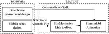
In virtual environment design, the environment and robot model design has different approach in MATLAB implementation. The environment design process starts with designing the environment using SolidWorks and then converted into VRML file. The VRML file can be further edited using V-Realm application embedded in MATLAB. For mobile robot design, the process starts with SolidWorks design and then converted into MATLAB Simulink model using SimMechanics plugin installed inside SolidWorks application. The overall process in designing the virtual environment is shown in Figure 2.
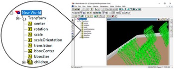
Based upon Figure 2, the virtual environmental process was divided into different software environments: SolidWorks and MATLAB. The environment and the mobile robot were properly designed with real parameters. They were used later in the model’s initialisation. For the environmental editing, this was modified in terms of rotation and translation and it needed to be properly inserted into the Simulink 3D Animation. Figure 3 shows the V-Realm software interface and the environmental translation. The rotation was modified in the Transform Group.
V-Realm software interface.

When designing the mobile robot model, the ‘mate features’ in the SolidWorks software for the assembly design needed to be identified and needed to be initialised carefully, as the Simulink conversion was computed based upon the joints that were initialised in the SolidWorks software. The joint directions were defined as a motion of follower’s frame relative to the base frame. Therefore, it was important to verify the joint types in the generated model, in order to avoid any unwanted motion during the simulation. After the environment and the robot model were combined, the overall environment was able to be edited using the 3D World Editor that is embedded inside the MATLAB software.
Results and Discussion
In this section, the results of designing the virtual environment and the robot’s navigational experiment are presented. The unicycle-like mobile robot model and the greenhouse environment with 4 different crop rows were designed by using the SolidWorks software. The navigational experiments were conducted in order to choose the best trajectories for the greenhouse navigation. The turning efficiency was calculated based upon the performances of each turn for each objective using the following formula:
 $${\rm }U_{{eff}} =\left( {{{\pi _{{err}} {\minus}U_{{err}} } \over {\pi _{{err}} }}{\plus}{{\pi _{{dist}} {\minus}U_{{dist}} } \over {\pi _{{dist}} }}{\plus}{{\pi _{{time}} {\minus}U_{{time}} } \over {\pi _{{time}} }}} \right){\times}100{\rm \,\%\,}$$
 $$\pi _{{eff}} =({{U_{{err}} {\minus}\pi _{{err}} } \over {U_{{err}} }}{\plus}{{U_{{dist}} {\minus}\pi _{{dist}} } \over {U_{{dist}} }}{\plus}{{U_{{time}} {\minus}\pi _{{time}} } \over {U_{{time}} }}){\times}100{\rm \,\%\,}$$
This is where U eff and π eff were the turning efficiencies, π err and U err were the total mean square tracking errors, π dist and U dist were the distances travelled and π time and U time were the time taken for π turn and U turn respectively. The positive values of turning efficiency shows the better trajectory performance in all objectives, respectively.
Mobile robot model
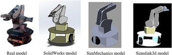
The unicycle-like mobile robot model was designed based on the real mobile robot system. It consists of two wheels and one castor wheel. It was equipped with Rhino XR-4 robot arm with 5 degrees of freedom. The model was design using the exact dimension as the real model to avoid model conflict and controller parameter problems in the hardware implementation. Figure 4 shows the mobile robot model that has been designed in SolidWorks and MATLAB respectively.
Designed mobile robot model.

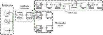
Based upon Figure 4, the mobile robot that was designed in SolidWorks was compatible for a MATLAB implementation, as the SimMechanicsTM Plugin was able to create a model that was based upon that design. The motion was then validated by simulating the SimMechanicsTM model. Figure 5 shows the Simulink block that was generated by SimMechanicsTM Plugin.
Generated mobile robot Simulink model.

Based upon Figure 5, the initialisation part of the generated model consisted of the world coordinates and they were then transformed into the robot’s coordinate system. The first part of the rigid body was a base for the mobile robot. The base consisted of three different revolute joints: the left wheel, the right wheel and the robot arm base. The robot arm base had a revolute joint, as it rotated about the z-axis. The arm revolute joints then continued until they reached the gripper body part. The joints were then able to rotate by using either the velocity or the position of the rotation. The wheels had different revolute joints, as the wheel rotations did not link with each other.
Virtual greenhouse environment
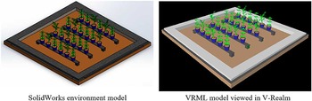
The virtual greenhouse environment was designed based upon a real greenhouse environment with dimensions of approximately 4.3 m x 4.5 m. Each row had a 3 m length and the row width varied according to the crop size. The designed environment consisted of 2 different crop types and they were arranged randomly in 4 different rows. Figure 6 shows the designed virtual environment.
Designed virtual environment.

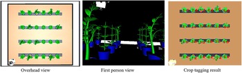
Based upon Figure 6, the designed SolidWorks model was then converted into a VRML file. In order to verify the conversion when comparing the VRML file with the SolidWorks model, V-Realm software was used. The environmental VRML file and the SimMechanicsTM mobile robot model were then combined inside the Simulink 3D environment. Figure 7 shows the Simulink 3D environment using different virtual camera views and the crop tagging results can be seen.
Simulink3d virtual environment result.

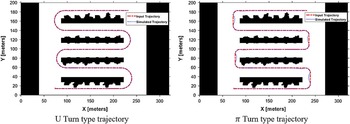
Figure 7 shows the results from a Simulink 3D animation view. In Simulink 3D, the camera views can be designed according to different positions with dissimilar orientations. For the navigational experiments, two camera views were used: an overhead view and a first-person view. Based upon the Figure, the crop tagging results show that the crops were identified successfully in the environment and they were named based upon the rows and the columns. The coordinates of the tagging processes were then transferred into the motion planner inputs in order to plan the motions according to the crop coordinate sequences. Figure 8 shows the motions that were computed by the Probabilistic Roadmap Planner.
Trajectory experiment result.

Based upon Figure 8, the path computed by the Probabilistic Roadmap Planner is shown by the dashed line and the simulated path is shown by the dotted line. The simulated path was computed by the mobile robot’s motion by using the feedback kinematic controller. The control parameters used were 2 for k x and k y and 0.5 for l x and l y , respectively. Figure 8 also proved that the controller was able to track the motion that was computed with a high degree of accuracy.
Table 1 shows the comparison that was computed between the U turn based trajectory and the π turn based trajectory. The comparisons were conducted based upon the travel time, the distance travelled and the controller mean square errors. The efficiency was calculated by using Equation 4 and 5 and by combining all of the criteria as stated. Based upon the table, the U turn based trajectory offered a better turning performance with 87.2% efficiency. It had a shorter distance that was travelled and lower trajectory errors. However, the time taken for the U turn was higher than it was for the π turn. The additional time was a result of the mobile robot’s speed depletion during the turning. As the U turn had a higher turning radius than did the π turn, the turning travel time was, therefore, higher. In addition, the controller also needed time to track the positions during the turning, as both of the x and y coordinates changed. However, the U turn would not be recommended to be implemented, if the time taken was the main criteria to be evaluated, as the π turn offered less time for the robot’s navigation.
Robot navigation simulation result.

When considering the π turn based trajectory assessment, it offered a higher distance travelled and more prominent controller errors. In terms of the distance travelled, the π turn covered a larger area than did the U turn, and thus, this contributed to the additional distance that was travelled. In terms of the controller errors, this was mainly because of the small turning radius. It was hard for the controller to track such a small change in positions. In order to reduce the errors, the alternatives of reducing the robot’s speed, or using a more complex controller, could be implemented and used. However, these alternatives would increase the travelling time, as the controller implementation would become more complex, and thus, it would make the turning more inefficient.
In terms of an overall comparison, the U turn based trajectory is recommended to be applied in an agricultural field with similar and minimum headland distance, as it provided for a better optimal path in agriculture. However, if the distance between headlands is high, π turn is recommended as it covers lower area and it was proved by Bochtis et al. (Reference Bochtis and Sorensen2009) where the π turn is executed when the turning radius is twice the machine minimum turning radius. Therefore, both turnings can be executed depending on the headlands distance and for minimum headland distance, U turn was recommended.
By using virtual reality as the programming environment, researchers especially in agriculture can visualize and validate their experiment findings and methodology with a clearer perspective. In this paper, the experiment was executed successfully as the robot motion can be observed clearly in the virtual environment. The controller parameter can also be tuned without using any hardware. The designed virtual environment that visualize the real environment will give benefits to the researcher to conduct experiment by using the same environment but executed in a very comfortable way.
Conclusions
In summary, the greenhouse virtual environment that employed 2 crop types was designed and simulated by MATLAB software. The mobile robot’s navigational experiments were conducted by using the Probabilistic Roadmap Planner and the trajectory performances were evaluated. The simulation results have shown that the U turn based trajectory is to be recommended, as it offered a lower distance travelled with lower tracking errors and with 82.7% efficiency. The method of using a virtual environment as an alternative method of conducting navigational experiments was a success, as the mobile robot’s motion was able to be simulated in the environment. For future works, a hardware implementation will be conducted and the trajectory performances will be evaluated and compared, in order to validate the best of operations.
Acknowledgement
The authors are grateful to the University of Technology Malaysia, the Ainuddin Wahid Scholarship and the Ministry of Higher Education (MOHE), for their partial financial support through their research funds, Vote No. R.J130000.7823.4F759.