2. Layer structure and scaling of ZPG TBL

In this study, we focus on statistically steady, two-dimensional incompressible flow. The mean-momentum equation in the streamwise $x\hbox{-}$ direction is given by (see Townsend Reference Townsend1956; Schlichting Reference Schlichting1979; Wei et al. Reference Wei, Li and Wang2024)

(2.1) \begin{align} 0 = - \left ( U \frac {\partial U}{\partial x} + V \frac {\partial U}{\partial y} \right ) \;\; {-\frac {1}{\rho }\frac {\partial P}{\partial x}} \;+\: {\nu \frac {\partial ^2 U}{\partial y^2}} \;+\; {\frac {\partial R_{\textit{uu}}}{\partial x} \;+\; \frac {\partial R_{\textit{uv}}}{\partial y}} , \end{align}

where $ \rho$ is the fluid density and $ \nu$ is the kinematic viscosity. Mean velocity and pressure are denoted by uppercase letters, while fluctuating velocity components are represented by lowercase letters. $U$ and $V$ denote the mean velocity components in the streamwise ( $x$ ) and wall-normal ( $y$ ) directions, respectively, and $u$ and $v$ denote the corresponding fluctuating components. Here, $ P = P(x, y)$ refers to the local mean pressure, highlighting that $ \partial P/\partial x$ is not assumed constant in the $y$ -direction, unlike in the classical thin boundary layer approximation. This distinction is important, as the assumption $ (1/\rho )\partial P/\partial x = - U_e \textrm {d}U_e/\textrm {d}x$ breaks down under strong adverse pressure gradients and near separation (Wei et al. Reference Wei, Li and Wang2024). The Reynolds normal stress is defined as $ R_{\textit{uu}} = - \langle u u \rangle$ , and the Reynolds shear stress as $ R_{\textit{uv}} = - \langle u v \rangle$ , where angle brackets denote Reynolds averaging. Neglecting the Reynolds stress terms reduces the momentum equation to its laminar form. The terms in (2.1) represent the balance among contributions from advection, pressure gradient, viscous diffusion and turbulent transport.

In layer II of the four-layer structure proposed by Wei et al. (Reference Wei, Fife, Klewicki and McMurtry2005), the force balance is primarily between the viscous force and the gradient of the Reynolds shear stress

(2.2) \begin{equation} 0 \approx \nu \frac {\partial ^2 U}{\partial y^2} \;+\; \frac {\partial R_{\textit{uv}}}{\partial y} .\end{equation}

It is widely accepted that the appropriate scales in the near-wall region (layers I and II) are the friction velocity, $ u_\tau$ , and the viscous length scale, $ \nu /u_\tau$ (see, e.g. Monin & Yaglom Reference Monin and Yaglom1965; Tennekes & Lumley Reference Tennekes and Lumley1972). Using these scales, the dimensionless variables are conventionally defined as follows: the inner-scaled distance from the wall, $ y^+ = y/(\nu /u_\tau )$ ; the inner-scaled velocity, $ U^+ = U/u_\tau$ ; and the inner-scaled Reynolds shear stress, $ R^+_{\textit{uv}} = R_{\textit{uv}}/u_\tau ^2$ . With these definitions, the inner-scaled mean-momentum equation for a ZPG TBL can be expressed as

(2.3) \begin{equation} 0 \approx \left [ \frac {\nu }{u^3_\tau } \right ] \left ( \nu \frac {\partial ^2 U}{\partial y^2} \right ) \;+\; \left [ \frac {\nu }{u^3_\tau } \right ] \frac {\partial R_{\textit{uv}}}{\partial y}, \quad \mathrm{or} \quad 0 \approx \frac {\partial ^2 U^+}{\partial (y^+)^2} \;+\; \frac {\partial R^+_{\textit{uv}}}{\partial y^+} .\end{equation}

The inner-scaled terms in the mean-momentum equation are presented in figure 1(a), using direct numerical simulation (DNS) data from Schlatter & Örlü (Reference Schlatter and Örlü2010) at two Reynolds numbers, ${\textit{Re}}_\theta =1000$ and ${\textit{Re}}_\theta =4060$ . To more clearly depict the near-wall region, the plot is shown on log–linear axes. Figure 1(a) shows that the force balance in the near-wall region is established between the viscous force and the gradient of the Reynolds shear stress. Moreover, the figure demonstrates an excellent collapse of the data from the two Reynolds numbers. Overall the figure supports the validity of the traditional inner scaling in the near-wall region. Notably, figure 1(a) shows that the viscous force and the gradient of Reynolds shear stress both reach their maximum magnitudes of approximately $0.07$ at $y^+ \approx 7$ , independent of Reynolds numbers.

In layer IV of a ZPG TBL, the dominant force balance shifts to one between the advective terms and the gradient of the Reynolds shear stress (Wei et al. Reference Wei, Fife, Klewicki and McMurtry2005)

(2.4) \begin{equation} 0 \approx - \left ( U \frac {\partial U}{\partial x} + V \frac {\partial U}{\partial y} \right ) \;+\; \frac {\partial R_{\textit{uv}}}{\partial y} .\end{equation}

Traditional outer scaling for the gradient of the Reynolds shear-stress term is $u^2_\tau$ for $R_{\textit{uv}}$ and $\delta _e$ for $y$ . To satisfy the admissible scaling criterion within the scaling patch framework, the advective term must likewise scale as $u^2_\tau /\delta _e$ (Fife et al. Reference Fife, Klewicki, McMurtry and Wei2005a ). Accordingly, an appropriate outer scaling of the mean-momentum equation for ZPG TBLs is given by

(2.5) \begin{equation} 0 \approx - \left [\frac {\delta _e}{u^2_\tau } \right ] \left ( U \frac {\partial U}{\partial x} + V \frac {\partial U}{\partial y} \right ) \;+\; \left [\frac {\delta _e}{u^2_\tau } \right ]\frac {\partial R_{\textit{uv}}}{\partial y} .\end{equation}

This traditional outer scaling of the mean-momentum equation is shown in figure 1(b) using the DNS data of a ZPG TBL by Schlatter & Örlü (Reference Schlatter and Örlü2010). The figure demonstrates excellent collapse of the data at two Reynolds numbers. As expected from the definition of a maximum, the zero-crossing point of the Reynolds shear-stress gradient coincides with the Reynolds shear-stress peak location, $y_m$ . For a more detailed discussion of the properties of ZPG TBLs, readers are referred to Wei et al. (Reference Wei, Fife, Klewicki and McMurtry2005) and Wei, Li & Wang (Reference Wei, Li and Wang2023).

Figure 1.

(a) Traditional inner scaling of the mean-momentum balance (MMB) for ZPG TBLs. (b) Traditional outer scaling of the MMB for ZPG TBLs. Data are from the DNS of Schlatter & Örlü (Reference Schlatter and Örlü2010) at ${\textit{Re}}_\theta = 1000$ (filled markers) and ${\textit{Re}}_\theta =4060$ (open markers).

Recently, Wei & Knopp (Reference Wei and Knopp2023) introduced a new outer scaling for TBLs subjected to pressure gradients. In this framework, the characteristic outer length scale is given by $ \delta _e - y_m$ , and the outer velocity scale is $ \sqrt {R_{\textit{uv}}|_{\textit{max}}}$ . Under this scaling, the dimensionless mean-momentum equation for the outer layer takes the form

(2.6) \begin{equation} 0 \approx - \left [\frac {\delta _e - y_m}{R_{\textit{uv}}|_{\textit{max}}} \right ] \left ( U \frac {\partial U}{\partial x} + V \frac {\partial U}{\partial y} \right ) \;+\; \left [\frac {\delta _e - y_m}{R_{\textit{uv}}|_{\textit{max}}} \right ] \frac {\partial R_{\textit{uv}}}{\partial y} .\end{equation}

The new outer scaling of the mean-momentum equation for ZPG TBLs is shown in figure 2. By construction, the zero crossing of the normalised Reynolds shear-stress gradient occurs at the origin of the figure, a direct consequence of using the normalised wall-normal coordinate $(y-y_m)/(\delta _e - y_m)$ .

Figure 2.

New outer scaling of the MMB for ZPG TBLs. Data are from the DNS of Schlatter & Örlü (Reference Schlatter and Örlü2010) at ${\textit{Re}}_\theta = 1000$ (filled markers) and ${\textit{Re}}_\theta =4060$ (open markers).

In ZPG TBLs, it is known that $y_m \sim \sqrt {\delta _e \nu / u_\tau }$ or $y^+_m \sim \sqrt {{\textit{Re}}_\tau }$ (see, e.g. Long & Chen Reference Long and Chen1981; Afzal Reference Afzal1982; Sreenivasan & Sahay Reference Sreenivasan and Sahay1997; Wei et al. Reference Wei, Fife, Klewicki and McMurtry2005; Wei Reference Wei2018; Romero et al. Reference Romero, Zimmerman, Philip, White and Klewicki2022a ; Smits Reference Smits2022). Additionally, the difference between $ R_{\textit{uv}}|_{\textit{max}}$ and $ u^2_\tau$ diminishes with increasing Reynolds number, following $ u^2_\tau - R_{\textit{uv}}|_{\textit{max}} \sim u^2_\tau /\sqrt {{\textit{Re}}_\tau }$ (Fife et al. Reference Fife, Wei, Klewicki and McMurtry2005b ). As a result, at sufficiently high Reynolds numbers, $ y_m \ll \delta _e$ and $ R_{\textit{uv}}|_{\textit{max}} \approx u^2_\tau$ , so that the outer scaling proposed by Wei & Knopp (Reference Wei and Knopp2023) asymptotically reduces to the classical outer scaling. For instance, at the two Reynolds numbers shown in figure 1(b), the ratio $y_m/\delta _e$ is $0.11$ and $0.05$ for ${\textit{Re}}_\theta =1000$ and ${\textit{Re}}_\theta =4060$ , respectively, while $R^+_{\textit{uv}}|_{\textit{max}}$ is approximately $0.90$ and $0.95$ for these cases. Consequently, the new outer scaling shown in figure 2 closely matches the traditional outer scaling presented in figure 1(b).

However, for TBLs subjected to pressure gradients, particularly under strong APG conditions, $y_m$ is not much smaller than $\delta _e$ , and $R_{\textit{uv}}|_{\textit{max}}$ can deviate significantly from $\tau _{w\textit{all}}/\rho$ (as shown in figure 3). Under these conditions, the traditional outer scaling becomes invalid, necessitating the adoption of the new outer scaling proposed by Wei & Knopp (Reference Wei and Knopp2023). In the following sections, we use the scaling patch approach to identify the layer structure of TBLs where pressure gradients affect the flow characteristics.

3. Layer structure and scaling in TBLs under pressure gradients

To demonstrate the application of the scaling patch analysis to the mean-momentum equation in TBLs under pressure gradients, we primarily use the DNS data from Coleman, Rumsey & Spalart (Reference Coleman, Rumsey and Spalart2018). A brief summary of the flow configuration is provided here; further details can be found in the original publication. In their study, Coleman et al. (Reference Coleman, Rumsey and Spalart2018) simulated non-equilibrium TBLs subjected sequentially to an adverse pressure gradient followed by a favourable pressure gradient (FPG). The pressure gradients were imposed via a prescribed transpiration velocity profile, $V_{\textit{top}}(x)$ , applied at a virtual parallel plane located at a fixed wall-normal distance $Y$ above the flat no-slip surface. The archived dataset, available from NASA TMR, is normalised using $Y$ as the reference length scale and $U_{_0} = U_e(x_0)$ as the reference velocity.

Figure 3(a) presents the streamwise variation of the free-stream velocity, wall shear stress $\tau _{w\textit{all}}/\rho$ and maximum Reynolds shear stress, while figure 3(b) shows the corresponding streamwise variations of the pressure gradients $(1/\rho )\textrm {d}P_{w\textit{all}}/\textrm {d}x$ and $(1/\rho )\textrm { d}P_e/\textrm {d}x$ . According to the mean-momentum equation at the boundary layer edge, the external pressure gradient is related to the streamwise velocity gradient as $(1/\rho )\textrm {d}P_e/\textrm {d}x = - U_e \textrm {d}U_e/\textrm {d}x$ . The wall shear stress in figure 3(a) indicates that the flow separates at $x/Y \approx -1.4$ and re-attaches at $x/Y \approx 0.4$ . Within the separated flow region, the wall shear stress becomes negative, corresponding to a negative skin-friction coefficient. Notably, figure 3(b) shows that the pressure gradient is relatively mild in the vicinity of separation zone $-1 \lesssim x/Y \lesssim 1$ .

Figure 3(a) also shows that the maximum Reynolds shear stress and wall shear stress have comparable magnitudes around the inlet and outlet of the simulation domain, where the pressure gradient is weak. However, in regions with strong pressure gradients or near the separation zone, the maximum Reynolds shear stress deviates significantly from the wall shear stress.

Figure 3.

(a) Streamwise variation of the $U_e$ , wall shear stress and maximum Reynolds shear stress in the DNS dataset of Coleman et al. (Reference Coleman, Rumsey and Spalart2018). To enhance visualisation, the wall shear stress and maximum Reynolds shear stress are multiplied by a factor of 500. (b) Streamwise variation of the pressure gradient.

Figure 3(b) shows that the magnitude of the pressure gradient peaks at $x/Y = -4$ in the APG region and at $x/Y = 4$ in the FPG region. Importantly, the figure indicates that the free-stream pressure gradient, $\textrm {d}P_e/\textrm {d}x$ , differs significantly from the wall pressure gradient, $\textrm {d}P_{w\textit{all}}/\textrm {d}x$ , in regions where the pressure gradient undergoes rapid changes or where the flow is reversed. Interestingly, the wall pressure gradient remains approximately constant in the reversed flow region, while the free-stream pressure gradient decreases monotonically in this simulation. Outside of these regions, the two gradients closely coincide. This distinction between the two pressure gradients plays a critical role in the momentum equation and its integral formulation, as discussed in Wei et al. (Reference Wei, Li and Wang2024).

Despite extensive research, no universally accepted dimensionless parameter has been established to effectively characterise the influence of pressure gradients on the development of TBLs. Several dimensionless pressure-gradient parameters have been proposed in the literature, and a summary of these is provided in table 1.

Table 1.

Commonly used parameters for pressure gradient in turbulent boundary layer flows. Here, ${\textit{Re}}_\theta = U_e \delta _2/\nu$ is the momentum thickness Reynolds number; ${\textit{Re}}_\tau = |u_\tau | \delta _e/\nu$ is the friction Reynolds number or Karman number; $C_{\!f} = \tau _{w\textit{all}}/(0.5\rho U^2_e)$ is the friction coefficient; $H_{12}=\delta _1/\delta _2$ is the shape factor; and $U_{_{{ZS}}}$ is the Zagarola–Smits velocity.

Figure 4 presents the streamwise variation of the commonly used pressure-gradient parameters, $\beta _{{_{\textit{RC}}}}$ and Stratford–Mellor inner pressure-gradient parameter $\beta _{\textit{in}}$ , based on the simulation data from Coleman et al. (Reference Coleman, Rumsey and Spalart2018). For ease of comparison within a limited vertical axis range, $\beta _{{_{\textit{RC}}}}$ is multiplied by a factor of 0.01. By definition, both parameters approach infinity near the separation points at approximately $x/Y \approx -1.4$ and $x/Y \approx 0.4$ . Within the reversed flow region ( $-0.8 \lt x/Y \lt 0$ ), the inner pressure-gradient parameter $\beta _{\textit{in}}$ remains nearly constant at −0.7, while $\beta _{{_{\textit{RC}}}}$ also exhibits a nearly constant behaviour but with a significantly larger magnitude of approximately $-130$ .

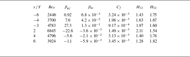
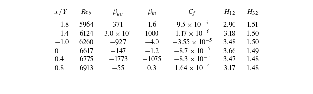
For clarity and brevity, we present the scaling of the MMB equations at a set of representative streamwise locations. These include six points located away from the separation region and six points in the vicinity of separation. The key parameters for these locations are summarised in table 2 and table 3. This targeted selection enables a detailed examination of how the scaling behaviour evolves across varying pressure-gradient conditions, providing clear insights into the dynamics both away from and near the separation region.

3.1. Outer scaling of TBLs under pressure gradients

In the outer region of TBLs, viscous forces become negligible, and the force balance is primarily dictated by the interplay of advective, turbulent and, when significant, pressure forces. Figure 5(a) illustrates the force distributions at $x/Y=-4$ , where the flow experiences the largest APG magnitude. In the outer region of boundary layer at this $x-$ location, the pressure force exceeds the turbulent forces by approximately an order of magnitude. However, this $x-$ location is situated far from the separation point, with a non-negligible wall shear stress. As a result, the dimensionless pressure-gradient parameters are not excessively large, with values of $\beta _{{_{\textit{RC}}}} \approx 7$ and $\beta _{\textit{in}} \approx 0.04$ .

Table 2.

Reynolds number and pressure-gradient parameters at locations away from separation zone in the DNS of Coleman et al. (Reference Coleman, Rumsey and Spalart2018).

Table 3.

Reynolds number and pressure-gradient parameters at locations in the vicinity of separation from the DNS of Coleman et al. (Reference Coleman, Rumsey and Spalart2018).

Figure 4.

Streamwise variation of the dimensionless pressure-gradient parameters, $\beta _{{_{\textit{RC}}}}$ and $\beta _{{\textit{in}}}$ , in the DNS of Coleman et al. (Reference Coleman, Rumsey and Spalart2018).

As shown in figure 5(a), under strong pressure gradients, the advective force in the outer region nearly counterbalances the pressure force, while other forces play a negligible role. However, a scaling patch analysis based solely on this balance fails to account for the contribution of the Reynolds stresses gradient, which is known to significantly influence the flow dynamics in the outer region.

The mean streamwise velocity deficit, $U_e - U$ , is widely recognised as a more meaningful metric for assessing relative variation of streamwise velocity in the outer region. Accordingly, a proper formulation for the advective term in the outer layer is

(3.1) \begin{equation} - \left ( U \frac {\partial U}{\partial x} + V \frac {\partial U}{\partial y} \right ) = -\frac {1}{2}\frac {\partial (U_e -U)^2}{\partial x} + \frac {\partial (U_e (U_e -U))}{\partial x} + V \frac {\partial (U_e -U)}{\partial y} - U_e \frac {\textrm { d}U_e}{\textrm {d}x}. \end{equation}

Under strong pressure gradients, the component $U_e \textrm {d}U_e/\textrm {d}x$ in (3.1) becomes large and scales differently from the other components. To enable a consistent scaling patch analysis – where the turbulent force is comparable in magnitude to the advective and pressure terms – we propose redistributing $ U_e \, \mathrm{d}U_e/\mathrm{d}x$ from the advective term into the pressure-gradient term, yielding a modified pressure term: $- ( ({1}/{\rho }) ( {\partial P}/{\partial x}) + U_e ({\textrm {d}U_e}/{\textrm {d}x}) )$ . The advective term is then reformulated as $- ( U ({\partial U}/{\partial x} )+ V ({\partial U}/{\partial y}) - U_e ({\textrm {d}U_e}/{\textrm {d}x}) )$ . This redistribution brings the advective and turbulent terms onto comparable scales, thereby facilitating a consistent scaling patch analysis under strong pressure-gradient conditions.

Figure 5.

(a) Traditional outer scaling of the MMB in TBLs under strong APG. (b) Traditional outer scaling of the MMB after redistribution. Data are from DNS of Coleman et al. (Reference Coleman, Rumsey and Spalart2018) at $x/Y=-4$ , where the pressure gradient has the largest magnitude. The dimensionless pressure-gradient parameters are $\beta _{{_{\textit{RC}}}} = 7.6$ and $\beta _{in}=0.042$ .

With the redistribution of $U_e ( {\textrm {d}U_e}/{\textrm {d}x})$ , the mean-momentum equation in the outer regions can be expressed as

(3.2) \begin{equation} 0 \approx - \left ( \frac {1}{\rho } \frac {\partial P}{\partial x} + U_e \frac {\textrm {d}U_e}{\textrm {d}x} \right ) - \left ( U \frac {\partial U}{\partial x} + V \frac {\partial U}{\partial y} - U_e \frac {\textrm {d}U_e}{\textrm {d}x}\right ) \;+\; {\frac {\partial R_{\textit{uu}}}{\partial x} \;+\; \frac {\partial R_{\textit{uv}}}{\partial y}}, \end{equation}

or equivalently, in terms of the mean streamwise velocity deficit

(3.3) \begin{align} 0 & \approx - \left ( \frac {1}{\rho } \frac {\partial P}{\partial x} + U_e \frac {\textrm {d}U_e}{\textrm {d}x} \right ) - \left ( \frac {1}{2} \frac {\partial (U_e - U)^2}{\partial x} - \frac {\partial (U_e(U_e-U))}{\partial x} - V \frac {\partial (U_e-U)}{\partial y} \right ) \nonumber \\[4pt] & \quad + {\frac {\partial R_{\textit{uu}}}{\partial x} + \frac {\partial R_{\textit{uv}}}{\partial y}} .\end{align}

The traditional outer scaling of the MMB equation, incorporating the redistribution, is shown in figure 5(b). After applying the redistribution, the advective term and the gradient of the Reynolds shear stress attain similar magnitudes. However, when scaled by $u^2_\tau$ as in traditional outer scaling, the magnitudes of both the advective term and the gradient of the Reynolds shear stress are approximately twice as large as their counterparts in ZPG TBLs. This discrepancy highlights the limitations of the traditional outer scaling for TBLs under pressure gradients.

Using the new outer scaling proposed by Wei & Knopp (Reference Wei and Knopp2023), the dimensionless mean-momentum equation for the outer region of TBLs under pressure gradient can be written as

(3.4) \begin{equation} 0 \approx - \frac {\left ( \dfrac {1}{\rho } \frac {\partial P}{\partial x} + U_e \dfrac {\textrm {d}U_e}{\textrm {d}x} \right )}{\dfrac {R_{\textit{uv}}|_{\textit{max}}}{\delta _e - y_m}} - \frac {\left ( U \dfrac {\partial U}{\partial x} + V \dfrac {\partial U}{\partial y} - U_e \dfrac {\textrm {d}U_e}{\textrm {d}x}\right )}{\dfrac {R_{\textit{uv}}|_{\textit{max}}}{\delta _e - y_m}} \;+\; \frac {\dfrac {\partial R_{\textit{uu}}}{\partial x}}{\dfrac {R_{\textit{uv}}|_{\textit{max}}}{\delta _e - y_m}} \;+\; \frac {\dfrac {\partial R_{\textit{uv}}}{\partial y}}{\dfrac {R_{\textit{uv}}|_{\textit{max}}}{\delta _e - y_m}}. \end{equation}

Figure 6 presents the terms in the MMB equation scaled using the new outer scaling. The results show comparable magnitudes for the reformulated advective term, the Reynolds shear-stress gradient and the Reynolds normal stress gradient. Furthermore, the new outer-scaled advective term and Reynolds shear-stress gradient in APG TBL closely resemble those in ZPG cases.

Figure 6.

New outer scaling of the MMB in TBLs under strong APG. Data are from the DNS of Coleman et al. (Reference Coleman, Rumsey and Spalart2018) at $x/Y=-4$ , where the pressure gradient has the largest magnitude.

Figure 7.

New outer scaling of TBLs under pressure gradients: (a,c,e) APG at $x/Y=-6, -4, -3$ , respectively; (b,d,f) FPG at $x/Y=6, 4, 2$ , respectively. The black + symbols represent the sum of all of the forces. Data are from the DNS by Coleman et al. (Reference Coleman, Rumsey and Spalart2018).

Figure 7 further validates the robustness of the new outer scaling by presenting results at three $x$ -locations within the APG region and three $x$ -locations within the FPG region. The corresponding flow parameters for these positions are listed in table 2. These selected locations are situated in regions experiencing strong pressure gradients but remain sufficiently distant from the separation zone. The Rotta–Clauser pressure-gradient parameter, $\mid\beta _{{_{\textit{RC}}}}\mid$ , varies between $0.92$ and $27.3$ , whereas the inner-scaled parameter $\beta _{in}$ remains consistently much smaller than $1$ . To confirm that the forces in the MMB are balanced, the sum of the forces is represented by + symbols, which aligns closely with zero. The minor scatter observed is attributed mainly to uncertainties in computing the $\partial /\partial x$ terms during postprocessing.

Figure 7(a) shows that, at $x/Y=-6$ , the terms of the viscous force, $-(\partial P/\partial x - \textrm { d}P_e/\textrm {d}x)$ , and $\partial R_{\textit{uu}}/\partial x$ are negligible. Consequently, the force balance in the outer region is primarily between the gradient of the Reynolds shear stress, $\partial R_{\textit{uv}}/\partial y$ , and the redistributed advective force, similar to the balance observed in ZPG TBLs. Figure 7(c) shows that, at $x/Y=-4$ , where APG reaches its maximum magnitude, the term $\partial R_{\textit{uu}}/\partial x$ becomes non-negligible. Figure 7(e,f) shows that, at $x/Y=-3$ and $x/Y=2$ , where the flow transitions rapidly from an APG to an FPG, the difference between $\textrm {d}P_e/\textrm {d}x$ and $\textrm {d}P_{w\textit{all}}/\textrm {d}x$ becomes significant. At these locations, $-(\partial P/\partial x - \textrm {d}P_e/\textrm {d}x)$ have magnitudes comparable to the peak value of $\partial R_{\textit{uv}}/\partial y$ , indicating its importance in the force balance (Wei et al. Reference Wei, Li and Wang2024).

Figure 8.

New outer scaling for TBLs in the vicinity of separation: (a,c,e) at $x/Y \approx -1.8, -1.4, -1.0$ ; (b,d,f) at $x/Y \approx 0, 0.4, 0.8$ . Data are from the DNS by Coleman et al. (Reference Coleman, Rumsey and Spalart2018).

To evaluate the effect of flow separation on the new outer scaling, figure 8 presents the new outer scaling applied at six $x$ -locations in the vicinity of separation. The relevant parameters for these locations are provided in table 3. The summation of forces, represented by black ‘+’ symbols in the figures, shows excellent agreement with zero, confirming the accuracy of both the simulation data and the postprocessing methodology. The results demonstrate that this new outer-scaling framework effectively captures the key interactions among forces in the outer region of TBLs, even in the presence of flow separation. While complete similarity cannot be expected due to the strong influence of pressure gradients and upstream flow history effects, the critical criterion is whether the proposed method accurately captures the appropriate scaling of the forces. The findings confirm that this scaling approach provides a robust framework for understanding force distributions in TBLs subjected to complex pressure-gradient conditions.

Figure 8(a,c,e) shows that $-(\partial P/\partial x - \textrm {d}P_e/\textrm {d}x)$ is positive inside TBL under APG, while the $\partial R_{\textit{uu}}/\partial x$ term is negative and exhibits a magnitude comparable to that of the $\partial R_{\textit{uv}}/\partial y$ term. Conversely, figure 8(b,d,f) shows that $-(\partial P/\partial x - \textrm {d}P_e/\textrm {d}x)$ is negative inside TBL under FPG, with the $\partial R_{\textit{uu}}/\partial x$ term being positive. Additionally, figure 8 shows that the new outer-scaled gradient of the Reynolds shear stress in TBLs under pressure gradients exhibits strong similarity in shape to that in ZPG TBLs, regardless of the strength of the pressure gradient or the presence of flow separation. On the other hand, the shape of the advective force after redistribution is strongly influenced by the presence of flow separation.

3.2. Inner layer of TBLs under pressure gradient

3.2.1. Inner scaling for $|\beta _{\textit{in}}| \ll 0.07$

Figure 9 presents the traditional inner scaling of the MMB at two $x$ -locations with small $\beta _{\textit{in}}$ magnitudes. At $x/Y=-6$ , where the flow is under an APG, the pressure-gradient parameters are $\beta _{{{\textit{RC}}}} \approx 0.92$ and $\beta _{\textit{in}}\approx 6.8 \times 10^{-3}$ . At $x/Y=6$ , where the flow is under FPG, these values are $\beta _{{{\textit{RC}}}} \approx -1.1$ and $\beta _{\textit{in}}\approx -5.9 \times 10^{-3}$ .

Figure 9.

Traditional inner scaling of TBLs under weak pressure gradients: (a) APG at $x/Y=-6$ ( $\beta _{\textit{in}}=6.8\times 10^{-3}$ ); (b) FPG at $x/Y=6$ ( $\beta _{\textit{in}}=-5.9\times 10^{-3}$ ). Data are from the DNS by Coleman et al. (Reference Coleman, Rumsey and Spalart2018).

Close to the wall, the no-slip boundary condition and the damping effect of viscosity dictate that both the mean-velocity components $U$ and $V$ require a finite distance to develop appreciable magnitudes. Consequently, the advective forces are negligible in the immediate vicinity of the wall. Therefore, the force balance in the inner region of TBLs under a pressure gradient can be approximated as

(3.5) \begin{equation} 0 \approx \nu \frac {\partial ^2 U}{\partial y^2} + \frac {\partial R_{\textit{uv}}}{\partial y}- \frac {1}{\rho } \frac {\partial P}{\partial x} .\end{equation}

This equation can be rewritten in non-dimensional form using traditional inner scales as

(3.6) \begin{equation} 0 \approx \frac {\partial ^2 U^+}{\partial (y^+)^2} + \frac {\partial R^+_{\textit{uv}}}{\partial y^+} - \frac {\nu }{ \rho u^3_\tau } \, \frac {\partial P}{\partial x}. \end{equation}

Note that the traditional inner-scaled pressure gradient can also be written as $({\nu }/{ \rho u^3_\tau }) \, ({\partial P}/{\partial x}) = \beta _{\textit{in}} \, (({{\partial P}/{\partial x})}/({ {\textrm {d}P_{w\textit{all}}}/{\textrm {d}x}}))$ . At $x=-6$ and $x=6$ in figure 9, the values of $\beta _{\textit{in}}$ are very small values. As a result, (3.6) can be further approximated to (2.3) for the inner region of ZPG TBLs.

3.2.2. Inner scaling of TBLs for $|\beta _{\textit{in}}| \gg 0.07$ : pressure–viscous force balance sub-layer

By definition, a large magnitude of $\beta _{\textit{in}}$ arises either under a very strong pressure gradient or near the separation point where $\tau _{w\textit{all}}$ approaches zero. Figures 3(b) and 4 show that, in the DNS data of Coleman et al. (Reference Coleman, Rumsey and Spalart2018), large values of $\beta _{\textit{in}}$ primarily occur near the separation points. Notably, at these locations, the pressure gradient itself is relatively small.

When $\tau _{w\textit{all}}$ approaches zero, the traditional inner-scaling framework based on $u_\tau$ and $\nu /u_\tau$ becomes invalid. This breakdown is evident in figure 10, which presents six locations where $|\beta _{\textit{in}}|$ is large. At the separation point ( $x/Y \approx -1.4$ ) and the re-attachment point ( $x/Y \approx 0.4$ ), the wall shear stress vanishes. Consequently, the traditionally inner-scaled viscous and pressure forces, normalised using $\nu /u^3_\tau$ , reach exceedingly large values $(\gt 1000)$ , clearly indicating the failure of the traditional inner scaling at these locations.

Figure 10.

Traditional inner scaling for TBL in the vicinity of separation: (a,c,e) at $x/Y \approx -1.8, -1.4, -1.0$ ; (b,d,f) at $x/Y \approx 0, 0.4, 0.8$ . Black + symbols denote the sum of all the forces in the MMB. Data are from the DNS by Coleman et al. (Reference Coleman, Rumsey and Spalart2018).

Figure 10 shows the existence of a near-wall sublayer in TBLs subjected to a pressure gradient, where the dominant balance is between the viscous force (blue symbols) and the pressure-gradient force (green symbols), consistent with earlier findings by Stratford (Reference Stratford1959) and Mellor (Reference Mellor1966). In this pressure–viscous force balance sub-layer, the MMB equation simplifies as follows:

(3.7) \begin{equation} 0 \approx \nu \frac {\partial ^2 U}{\partial y^2} - \frac {1}{\rho } \frac {\partial P}{\partial x}. \end{equation}

The corresponding boundary conditions are

(3.8) \begin{align} \nu \frac {\partial U}{\partial y}\Big |_{w\textit{all} = \frac {\tau _{w\textit{all}}}{\rho }; } \end{align}

(3.9) \begin{align} \nu \frac {\partial ^2 U}{\partial y^2}\Big |_{w\textit{all} = \frac {1}{\rho } \frac {\textrm {d} P_{w\textit{all}}}{\textrm {d}x}. } \end{align}

The controlling parameters for this sub-layer, derived from the boundary conditions and governing equations, are

(3.10) \begin{equation} \frac {1}{\rho } \frac {\textrm {d}P_{w\textit{all}}}{\textrm {d}x}, \; \nu , \; \tau _{w\textit{all}}. \end{equation}

Since $\tau _{w\textit{all}}$ becomes zero at the separation point, it is unsuitable to use it as a characteristic scale. Instead, by using the first two controlling parameters as repeating variables, the length and velocity scales for this sub-layer can be derived as

(3.11) \begin{align}{l_{p\nu } = \frac {\nu ^{\frac {2}{3}}}{ \left|\frac {1}{\rho } \frac {\textrm {d}P_{w\textit{all}}}{\textrm {d}x}\right|^{\frac {1}{3}}} = |\beta _{\textit{in}}|^{-\frac {1}{3}} \frac {\nu }{|u_\tau |} ,} \end{align}

(3.12) \begin{align}{ u_{\!p\nu } = \left |\frac {\nu }{\rho } \frac {\textrm {d}P_{w\textit{all}}}{\textrm {d}x} \right |^{\frac {1}{3}} = |\beta _{\textit{in}}|^{\frac {1}{3}} |u_\tau |. \\[9pt] \nonumber } \end{align}

These scales are fundamentally equivalent to those proposed by Stratford (Reference Stratford1959), who used $({1}/{\rho })({\partial \tau }/{\partial y})|_0$ instead of $({1}/{\rho }) ({\textrm {d}P_{w\textit{all}}}/{\textrm {d}x})$ , and Mellor & Gibson (Reference Mellor and Gibson1966) who employed $({1}/{\rho }) ({\textrm {d} P}/{\textrm {d} x})$ without specifying whether the pressure gradient was at the wall or at the boundary layer edge. Recently, Wei et al. (Reference Wei, Li and Wang2024) demonstrated that the pressure gradient ${\partial P}/{\partial x}$ varies in the wall-normal direction in TBLs subjected to strong pressure gradients. In this context, we emphasise the use of $({1}/{\rho }) ({\textrm {d}P_{w\textit{all}}}/{\textrm {d}x})$ as it directly represents a wall boundary condition for the governing equation. Furthermore, to properly define the characteristic length scales $u_{\!p\nu }$ and $l_{p\nu }$ for both positive and negative $\textrm {d}P_{w\textit{all}}/\textrm {d}x$ , it is essential to use the absolute value of the pressure gradient (or $|\partial \tau /\partial y|$ ) to ensure consistency in scaling.

The Stratford–Mellor inner-scaled variables relate to the traditional inner scaling as follows:

(3.13) \begin{align}{ y^* = \frac {y}{l_{p\nu }} = \mathrm{sgn}(\tau _{w\textit{all}})|\beta _{\textit{in}}|^{\frac {1}{3}} y^+ ,}\end{align}

(3.14) \begin{align}{ U^* = \frac {U}{u_{\!p\nu }} = \mathrm{sgn}(\tau _{w\textit{all}})|\beta _{\textit{in}}|^{-\frac {1}{3}} U^+. }\end{align}

Note that in the reversed flow region, $\tau _{w\textit{all}}$ is negative.

The DNS data indicate that the mean pressure gradient in the near-wall region is approximately constant, i.e. $({\partial (P/\rho )}/{\partial x}) \approx \textrm {d}(P_{w\textit{all}}/\rho )/\textrm {d}x$ (see figure 10). Hence, normalising (3.7) by $|\textrm {d}(P_{w\textit{all}}/\rho )/\textrm {d}x$ yields a dimensionless mean-momentum equation in the pressure–viscous sub-layer as (see also Skote & Henningson Reference Skote and Henningson1999 and Manhart et al. Reference Manhart, Peller and Brun2008)

(3.15) \begin{equation} 0 \approx \mathrm{sgn}\left(\frac {\textrm {d}P_{w\textit{all}}}{\textrm {d}x}\right) \frac {\partial ^2 U^*}{\partial (y^*)^2} - 1 \qquad \mathrm{or} \qquad 0 \approx \frac {1}{\beta _{\textit{in}}} \frac {\partial ^2U^+}{\partial (y^+)^2} - 1 .\end{equation}

Figure 11 presents the Stratford–Mellor inner scaling at the six $x$ -locations listed in table 3. By definition, such inner-scaled viscous and pressure forces attain a magnitude of one in the immediate vicinity of the wall. Furthermore, the thickness of this sublayer is approximately $y/l_{p\nu } \approx 1$ .

Figure 11.

New inner scaling of TBLs in the vicinity of separation: (a,c,e) at $x/Y \approx -1.8, -1.4, -1.0$ ; (b,d,f) at $x/Y \approx 0, 0.4, 0.8$ . The black + symbols represent the sum of all the forces in the MMB. Data are from the DNS by Coleman et al. (Reference Coleman, Rumsey and Spalart2018).

3.3. Overlap layer: balance of viscous, pressure and Reynolds shear-stress gradients

As the distance from the wall increases, the viscous force diminishes while the gradient of Reynolds shear stress increases. Meanwhile, the pressure gradient remains nearly constant. Consequently, within a short distance from the wall, a force balance is established among the viscous force, pressure force and the gradient of Reynolds shear stress, as expressed in (3.5).

To examine the relative contributions of these terms, we normalise (3.5) by $\textrm { d}(P_{w\textit{all}}/\rho )/\textrm {d}x$ , yielding

(3.16) \begin{equation} 0 \approx \frac {1}{\beta _{\textit{in}}} \frac {\nu \dfrac {\partial ^2U}{\partial y^2}}{\dfrac {u^3_\tau }{\nu }} + \left [\frac {1}{\rho }\frac {\textrm {d}P_{w\textit{all}}}{\textrm {d}x}\right ]^{-1} \,\frac {\partial R_{\textit{uv}}}{\partial y} - 1. \end{equation}

The viscous force in the near-wall region closely responds to the pressure force, allowing these two terms to be combined. Figure 12 illustrates this combined force for two locations near the separation points. At other locations, the force balance between the gradient of the Reynolds shear stress and the combined pressure and viscous forces exhibits a similar behaviour.

Figure 12.

New inner scaling of forces, combining the pressure and viscous forces: (a) at $x/Y = -1.4$ ( $\beta _{\textit{in}}=1000$ ); (b) at $x/Y = 0.4$ ( $\beta _{\textit{in}}=-1075$ ). Data are from the DNS by Coleman et al. (Reference Coleman, Rumsey and Spalart2018).

3.3.1. Sub-layer with linear growth of Reynolds shear stress

Figure 11(b,d) reveals the presence of a distinct sub-layer, in which the force balance is primarily between the pressure force and the gradient of the Reynolds shear stress. This region emerges as the viscous force rapidly diminishes outside the pressure–viscous sub-layer, while the advective term has not yet become significant. Notably, within this near-wall region, the pressure force remains nearly constant, leading to a corresponding constancy in the gradient of the Reynolds shear stress

(3.17) \begin{equation} 0 \approx \left [\frac {1}{\rho }\frac {\textrm {d}P_{w\textit{all}}}{\textrm {d}x}\right ]^{-1} \,\frac {\partial R_{\textit{uv}}}{\partial y} -1 , \end{equation}

which leads to a linear growth of the Reynolds shear stress in this sub-layer

(3.18) \begin{equation} \frac {R_{\textit{uv}}}{u^2_{p\nu }} \approx \frac {y}{l_{p\nu }} + c \qquad \mathrm{or} \qquad R^+_{\textit{uv}} \approx \beta _{\textit{in}} y^+ + c. \end{equation}

Figure 13 illustrates the linear growth of Reynolds shear stress at the streamwise location of $x/Y=0.4$ , with the layer thickness approximately $O(10 l_{p\nu })$ . While previous studies (e.g. Perry et al. Reference Perry, Bell and Joubert1966) have reported such linear growth regions in pressure-gradient TBLs, the conditions for their existence have remained unclear. Figure 13 also shows that within the pressure–viscous sublayer, the growth of Reynolds shear stress is negligible, and beyond the linear growth region, its increase gradually slows. However, the maximum Reynolds shear stress remains within the same order of magnitude as its value at the end of the linear growth region, being less than twice as large.

Figure 13.

Linear growth of Reynolds shear stress in the near-wall region. The Reynolds shear stress and wall-normal distance are normalised using Stratford–Mellor inner scales. Data are from the DNS of Coleman et al. (Reference Coleman, Rumsey and Spalart2018) at $x/Y = 0.4$ ( $\beta _{\textit{in}}=-1075$ ).

To further investigate the characteristics of the forces in the MMB equation and the shape of the Reynolds shear-stress profile, figure 14 presents the Stratford–Mellor inner-scaled Reynolds shear stress alongside the MMB terms at four $ x$ -stations. The stations at $ x/Y = -2$ and 0.5 correspond to the locations where $ \beta _{\textit{in}}$ attain the value of 0.7 before the separation point $x/Y=-1.4$ and after the re-attachment point $x/Y=0.4$ . The stations at $ x/Y = -0.5$ and $ x/Y = 0$ lie within the reversed flow region, where $ |\beta _{\textit{in}}| \gtrsim 0.7$ .

Figure 14.

Stratford–Mellor inner-scaled Reynolds shear stress and terms in the MMB equation (data symbols correspond to those in figure 11). (a,b,c,d) at $x/Y=-2, -0.5, 0, 0.5$ , respectively. Data are from the DNS by Coleman et al. (Reference Coleman, Rumsey and Spalart2018).

To assess the relationship between the maximum Reynolds shear stress, $ R_{\textit{uv}}|_{\textit{max}}$ , and the pressure–viscosity velocity scale, $ u_{\!p\nu }$ , figure 15 presents the streamwise variation of $ R_{\textit{uv}}|_{\textit{max}}/u^2_{p\nu }$ alongside the Stratford–Mellor inner pressure-gradient parameter, $ \beta _{\textit{in}}$ . For reference, the horizontal red line indicates $ \beta _{\textit{in}} = 0.7$ . Near the inlet, where the pressure gradient is weak, the Reynolds shear stress exhibits behaviour similar to that in ZPG TBLs, with $ R_{\textit{uv}}|_{\textit{max}} \sim u_\tau ^2$ . In this region, $ u_{\!p\nu }$ remains small, resulting in $ R_{\textit{uv}}|_{\textit{max}}/u^2_{p\nu }$ values well above 100. As the pressure gradient increases, $ R_{\textit{uv}}|_{\textit{max}}/u^2_{p\nu }$ decreases significantly, falling below 100. Approaching the separation zone at $ x/Y = -1.4$ , $ \beta _{\textit{in}}$ increases sharply, while $ R_{\textit{uv}}|_{\textit{max}}/u^2_{p\nu }$ fluctuates between approximately 50 and 130, as also shown in figures 13 and 14. The exceptionally large value observed at $ x/Y = 1.3$ corresponds to the location where $ \textrm {d}P_{w\textit{all}}/\textrm {d}x$ crosses zero. Overall, figure 15 highlights the relevance of $ u_{\!p\nu }$ in characterising the Reynolds shear stress in TBLs under strong pressure gradients or near separation, as evidenced by the nearly constant ratios in the separation zone.

Figure 15.

Streamwise variation of maximum Reynolds shear stress normalised by $u^2_{p\nu }$ and the $\beta _{\textit{in}}$ . The horizontal red dashed line indicates $\beta _{\textit{in}}=0.7$ . Data are from the DNS by Coleman et al. (Reference Coleman, Rumsey and Spalart2018).

4. Extended validation with simulation and experimental data of TBLs under pressure gradients

To further assess the robustness of the proposed scaling framework, we apply it to two independent datasets from Bobke et al. (Reference Bobke, Vinuesa, Örlü and Schlatter2017) and Kitsios et al. (Reference Kitsios, Sekimoto, Atkinson, Sillero, Borrell, Gungor, Jiménez and Soria2017), as well as two experimental datasets from Skåre & Krogstad (Reference Skåre and Krogstad1994) and Maciel, Rossignol & Lemay (Reference Maciel, Rossignol and Lemay2006). These cases encompass a wide range of Reynolds numbers, pressure-gradient strengths and upstream flow histories. The results demonstrate that the proposed scaling framework performs consistently across these diverse conditions, highlighting its generality and applicability to turbulent boundary layers subjected to arbitrary pressure gradients.

4.1. Large-eddy simulation results of Bobke et al. (Reference Bobke, Vinuesa, Örlü and Schlatter2017)

Bobke et al. (Reference Bobke, Vinuesa, Örlü and Schlatter2017) conducted a series of well-resolved large-eddy simulations (LES) to investigate TBLs under adverse pressure gradients. In their simulations, the pressure gradient was imposed by prescribing the free-stream velocity at the top of the computational domain using Townsend’s power-law formulation, $C (x-x_0)^m$ , where $C$ is a constant, $x_0$ denotes a virtual origin and $m$ is the power-law exponent (Townsend Reference Townsend1956; Mellor & Gibson Reference Mellor and Gibson1966). Five cases were simulated to explore different near-equilibrium boundary layers by varying the virtual origin and the power-law exponent: case m13 ( $x_0=60; m=-0.13$ ), case m16 ( $x_0=60; m=-0.16$ ), case m18 ( $x_0=60; m=-0.18$ ), case b1 ( $x_0=100; m=-0.14$ ) and case b2 ( $x_0=100; m=-0.18$ ). In cases b1 and b2, the Rotta–Clauser pressure-gradient parameter remains nearly constant throughout the simulation domain. Among all cases, the strongest pressure gradient – reflected by the highest value of the Rotta–Clauser parameter – occurs in case m18.

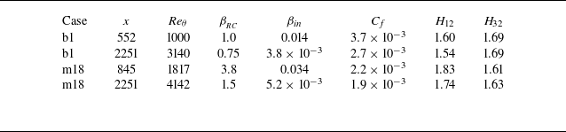
To concisely illustrate the proposed scaling, we present results at two representative streamwise locations for each of cases b1 and m18. The first location corresponds to the point of largest $\beta _{\textit{in}}$ , while the second is positioned at 90% of the simulation domain length from the inlet. Key parameters for these locations are summarised in table 4.

Table 4.

Parameters in the LES results of Bobke et al. (Reference Bobke, Vinuesa, Örlü and Schlatter2017).

Figure 16 presents the traditional inner scaling of simulation results. For case b1, the inner pressure-gradient parameter $\beta _{\textit{in}}$ remains small near both the inlet ( $\beta _{\textit{in}}=0.014$ ) and outlet ( $\beta _{\textit{in}}=3.8 \times 10^{-3}$ ). Consequently, the traditional inner scaling performs well, as shown in figures 16(a) and 16(c). For case m18, $\beta _{\textit{in}}$ is approximately $0.034$ near the inlet of the simulation domain, leading to noticeable deviations from the traditional inner-scaled behaviour of ZPG TBLs. However, near the outlet of the simulation domain in case m18, $\beta _{\textit{in}}$ decreases significantly to $5.2 \times 10^{-3}$ , well below 0.07. At this location, the traditionally inner-scaled force terms, shown in figure 16(d), becomes similar to those observed in ZPG TBLs.

Figure 16.

Traditional inner scaling of the force terms in the MMB from the LES study of Bobke et al. (Reference Bobke, Vinuesa, Örlü and Schlatter2017). Panels (a,c) show case b1 at streamwise locations $x=552$ ( $\beta _{\textit{in}} = 0.014$ ) and $x=2251$ ( $\beta _{\textit{in}} = 3.8 \times 10^{-3}$ ), respectively. (b,d) Case m18 at $x=845$ ( $\beta _{\textit{in}} = 0.034$ ) and $x=2251$ ( $\beta _{\textit{in}} = 5.2 \times 10^{-3}$ ), respectively.

Figure 17 presents the outer-scaling results for case b1 from Bobke et al. (Reference Bobke, Vinuesa, Örlü and Schlatter2017). In figures 17(a) and 17(c), the traditional outer scaling is applied at two $x$ -locations, showing significant deviations from the profiles observed in ZPG TBLs. In contrast, the new outer scaling, shown in figures 17(b) and 17(d), closely aligns with the scaling observed in ZPG TBLs. Similarly, figure 18 demonstrates the outer-scaling results for case m18 from Bobke et al. (Reference Bobke, Vinuesa, Örlü and Schlatter2017), exhibiting the same consistency with the new scaling framework.

Figure 17.

Outer scaling of the forces in the MMB for case b1 at $x=552$ and $x=2251$ from the LES study by Bobke et al. (Reference Bobke, Vinuesa, Örlü and Schlatter2017). (a,c) Traditional outer scaling. (b,d) New outer scaling.

Figure 18.

Outer scaling of the forces in the MMB for case m18 at $x=845$ and $2251$ from the LES study by Bobke et al. (Reference Bobke, Vinuesa, Örlü and Schlatter2017). (a,c) Traditional outer scaling. (b,d) New outer scaling.

4.2. Direct numerical simulation results of Kitsios et al. (Reference Kitsios, Sekimoto, Atkinson, Sillero, Borrell, Gungor, Jiménez and Soria2017)

Kitsios et al. (Reference Kitsios, Sekimoto, Atkinson, Sillero, Borrell, Gungor, Jiménez and Soria2017) conducted DNSs of self-similar turbulent boundary layers subjected to adverse pressure gradients for two cases. For the mild APG case, the nominal Rotta–Clauser pressure-gradient parameter was $\beta _{{{\textit{RC}}}} = 1$ ( ${\textit{Re}}_\theta = 3,100 - 3,440$ ), while in the strong APG case, $\beta {{_{\textit{RC}}}} \approx 39$ ( ${\textit{Re}}_\theta = 10\,000 - 12\,000$ ), approaching flow separation.

Figure 19 presents the traditional inner scaling of the force terms from the DNS dataset of Kitsios et al. (Reference Kitsios, Sekimoto, Atkinson, Sillero, Borrell, Gungor, Jiménez and Soria2017). Under mild APG, the normalised force distributions closely resemble those observed in ZPG TBLs. However, in the strong APG case (figure 19 b), the traditional inner-scaled forces deviate markedly from the ZPG TBLs profiles, underscoring the limitations of traditional inner scaling for such flows.

Figure 19.

Traditional inner scaling of results from DNS of Kitsios et al. (Reference Kitsios, Sekimoto, Atkinson, Sillero, Borrell, Gungor, Jiménez and Soria2017). (a) Mild APG case. (b) Strong APG case.

Figure 20 compares the traditional and new outer scaling applied to mild and strong APG cases from the same DNS dataset. For the mild APG, figure 20(a) shows that the traditionally scaled forces exceed those of the ZPG TBL by approximately a factor of 10. This discrepancy increases dramatically in the strong APG case, reaching a factor of approximately 200, as shown in figure 20(c). In contrast, the new outer scaling – shown in figures 20(b) and 20(d) – yields profiles that closely resemble those observed in ZPG TBLs, highlighting its effectiveness across varying pressure-gradient strengths.

Figure 20.

Outer scaling of the force terms from the DNS of Kitsios et al. (Reference Kitsios, Sekimoto, Atkinson, Sillero, Borrell, Gungor, Jiménez and Soria2017). (a,c) Traditional outer scaling for the mild and strong APG cases, respectively. (b,d) New outer scaling applied to the same two cases.

5. Summary

This study presents a systematic investigation of the effects of pressure gradients on the MMB in turbulent boundary layers using the scaling patch framework. By redistributing the component $U_e \textrm {d}U_e/\textrm {d}x$ from the advective term to the pressure-gradient term, we construct a revised scaling framework that remains consistent in the outer region – even under strong pressure gradients or near flow separation. The results show that the magnitudes of the reformulated advective and pressure forces become comparable to those of the Reynolds shear and normal stress gradients. This refined scaling patch analysis improves the outer-scaling framework proposed by Wei & Knopp (Reference Wei and Knopp2023), offering a unified perspective across a wide range of pressure-gradient conditions. Moreover, the gradient of Reynolds shear stress in pressure-gradient TBLs closely resembles its counterpart ZPG TBLs. The framework’s validity is supported by consistent results across multiple numerical simulations and experimental datasets spanning a broad range of Reynolds numbers, pressure gradients and upstream histories.

Figure 21.

New outer scaling of MMB using experimental data. (a) Experimental data of Maciel et al. (Reference Maciel, Rossignol and Lemay2006) at $x=1150$ mm ( ${\textit{Re}}_\theta = 5,486$ , $\beta _{{\textit{RC}}} = 9.3$ ). (b) Experimental data of Skåre & Krogstad (Reference Skåre and Krogstad1994) at the fifth station ( ${\textit{Re}}_\theta = 50,980$ , $\beta _{{\textit{RC}}} = 21.2$ ). For comparison, the ZPG TBL data are from DNS of Schlatter & Örlü (Reference Schlatter and Örlü2010) at ${\textit{Re}}_\theta =2000$ .

In the inner region, the effects of pressure gradient are found to be captured by the Stratford–Mellor parameter, $\beta _{\textit{in}}$ . When $|\beta _{\textit{in}}| \ll 0.07$ , traditional inner scaling using the friction velocity and viscous length scale remains valid. However, for $|\beta _{\textit{in}}| \gtrsim 0.07$ , the near-wall dynamics shifts to a pressure–viscous balance, with viscosity and the imposed wall pressure gradient dictating the relevant velocity and length scales. This regime aligns with the classical descriptions by Stratford (Reference Stratford1959) and Mellor (Reference Mellor1966).

Another important finding of this study is the clarification of a sub-layer where the Reynolds shear stress increases linearly with wall-normal distance. Although previous studies have observed this linear growth, the conditions and physical mechanism underlying the behaviour have remained unclear. This sub-layer, located beyond the immediate pressure–viscous balance region, is governed by a dominant balance between the imposed pressure gradient and the gradient of the Reynolds shear stress. It emerges when $|\beta _{\textit{in}}| \gtrsim 0.7$ and $\textrm {d}P_{w\textit{all}}/\textrm {d}x \gt 0$ . The linear variation of Reynolds shear stress in this region results from the near constancy of the pressure gradient and the negligible contribution of the mean-inertia term under these conditions.

These findings offer valuable insights into the structure and scaling of turbulent boundary layers under pressure gradients, enhancing the fundamental understanding of momentum transport mechanisms. The proposed framework lays the groundwork for improved turbulence modelling approaches that account for pressure-gradient effects, which are particularly relevant for aerodynamic applications, geophysical flows and engineering designs involving adverse pressure gradients.