1. Introduction

Total ice-volume monitoring is important for the observation of climatic change and its consequences such as global sea-level rise (Reference Jevrejeva, Moore and GrinstedJevrejeva and others, 2008). To estimate the total volume of stored water worldwide, UNESCO initiated the International Hydrological Decade (1965–74). In this context, systematic geophysical investigations on Austrian glaciers were started. In the years 1966–80, the total ice volumes of 15 glaciers were calculated based on ice depths derived from two-dimensional (2-D) seismic surveys (Reference Aric, Brückl., Hammerl, Lenhardt, Steinacker and SteinhausAric and Brü ckl, 2001).

First experiences with the radar technique on temperate alpine glaciers were gained in 1980/81 (Reference Haeberli, Wächter, Schmid and SidlerHaeberli and others, 1983). Progress in digital electronics, data acquisition and processing techniques led to the use of higher frequencies and consequently to higher resolution (Reference Blindow, and ThyssenBlindow and Thyssen, 1986; Reference Moran, Greenfield, Arcone and DelaneyMoran and others, 2000). Ground-penetrating radar (GPR) proved its suitability for glaciological use, and basic GPR applications also required less extensive fieldwork and data processing than other geophysical field techniques. Consequently, GPR gained in popularity and the number of investigated alpine glaciers increased (Reference Span, Fischer, Kuhn, Massimo and ButschekSpan and others, 2005). The economic and logistic constraints on surveys of remote glaciers meant that data density was often sparse and irregular, so it was seldom possible to calculate plausible results for ice-thickness distribution and total ice volume with standard interpolation techniques. As this is a common problem in less accessible regions, Reference Warner and BuddWarner and Budd (2000) introduced an approach to derive ice thickness and bedrock topography in data gap regions over Antarctica. This approach uses surface elevation data, ice-accumulation distributions via balance fluxes and basic assumptions about the dynamics of ice flow. Only a few Austrian glaciers are sufficiently well investigated to offer this data diversity. In this study, we present an interpolation approach for poorly data-covered regions using surface topography and GPR data to determine subglacial topography, ice-thickness distribution and total ice volume. Besides closing data gaps, the presented interpolation approach produces plausible ice-thickness distributions that can be used in glacier models. Numerical glacier modelling helps to clarify relevant physical processes underlying glacial response to climate change (Reference GreuellGreuell, 1992). Progress in modelling glacier dynamics, which has led from one-dimensional flowline models (Reference GreuellGreuell, 1992; Reference Wallinga and van de WalWallinga and Van de Wal, 1998) to models describing the three-dimensional (3-D) field of glacier flow (Reference Hubbard, Blatter, Nienow, Mair and HubbardHubbard and others, 1998; Reference GudmundssonGudmundsson, 1999), still crucially relies on accurate results of ice-thickness distribution.

2. Study Site

The two investigated glaciers are situated on the mountain Hoher Sonnblick (47^˚03^'16’’N, 12^˚57^'25’’ E; 3106m a.s.l.) in the Hohe Tauern region of the Eastern Alps in central Austria. The north-facing Goldbergkees has an area of 1.43 km² with an elevation range from 2380 to 3060 m; the south-facing Kleinfleisskees has an area of 0.87 km² with an elevation range from 2740 to 3060m (Reference Auer, Böhm, Schöner and LeymüllerAuer and others, 2002). Both are temperate glaciers and belong to the geomorphologic group of alpine valley glaciers. The Sonnblick climate observatory, which is situated on the summit (Fig. 1), has been in operation since 1886. Mass balance has been determined annually for Goldbergkees since 1988 and for Kleinfleisskees since 1998, and the average annual ice loss for both glaciers has been about 0.6m (ZAMG internal glacier database, 2008). Mass balance is determined by the standard glaciological method (Reference PatersonPaterson, 1994). As a result of climatic conditions in recent decades, firn coverage of the two glaciers is decreasing (Reference Auer, Böhm, Schöner and LeymüllerAuer and others, 2002). For the last 7 years the mean accumulation-area ratio (AAR; Reference BahrBahr, 1997) is about 0.35 (ZAMG internal glacier database, 2008).

Fig. 1.

The study site, in the Eastern Alps of central Austria. The black square marks the Sonnblick climate observatory, situated on the summit of Hoher Sonnblick mountain (3106ma.s.l.). The dashed line identifies the ice divide ‘Fleisscharte’ connecting the two parts of PP1 (Flk and Gok 1). The greyscale represents the picked bedrock reflection time data for PP1 and PP2. In this study, the term ‘bedrock reflection time’ denotes the one-way travel time of the GPR pulse reflected at the ice/bedrock boundary.

Since the 1970s, Goldbergkees has been divided into two parts (Gok 1 and Gok 2). The upper part (Gok 1) is connected via the ice divide ‘Fleisscharte’ with Kleinfleisskees (Flk). Because Gok 1 is connected to Flk and Gok 2 is now a separate glacier, we define two areas for processing purposes. Flk and Gok 1 comprise the first processing part (PP1), with an area of 1.26 km² and elevations ranging from 2740 to 3060 m. Gok 2 is the second processing part (PP2), with an area of 1.04 km² and elevations ranging from 2380 to 2780m (Fig. 1).

The most recent digital terrain model (DTM) for the investigated area is based on an aerial survey in autumn 1998 with a horizontal resolution of 10 m×10m (Reference Auer, Böhm, Schöner and LeymüllerAuer and others, 2002). This DTM 1998 was used to as a reference for elevations, ice thickness and topography of the glacier bed. Using differential global positioning system (DGPS) measurements of autumn 2005, we estimated mean elevation differences for the two glaciers in the period autumn 1998 to autumn 2005. Elevation differences for autumn 2004 were calculated using a linear approach. PP1 showed a mean elevation difference of –2m and PP2 a mean elevation difference of –5 m.

3. Data Acquisition and 2-d Processing

Weather conditions, inaccessibility, crevasses and the free water content of temperate glaciers restricted the time available for field surveys. The optimum compromise was the early springtime, the period of maximum accumulation. Mean measured snow depth is 3.5 m for PP1, and 4m for PP2. With respect to the different GPR propagation velocities of snow (~0.22mns^–1; Reference Frolov and MacheretFrolov and Macheret, 1999) and ice (v _ice = 0.167mns^–1; Reference Hubbard and GlasserHubbard and Glasser, 2005), total mean elevation differences for the two processing parts were calculated. Regarding the DTM 1998 and the snow cover of early spring 2004, the total mean elevation differences result in elevation corrections of +1m for PP1, and –2m for PP2.

The Subsurface Interface Radar (SIR)-2 system (Geophysical Survey Systems Inc. (GSSI)) was used for data acquisition. The antenna used was the unshielded multi-low-frequency (MLF) 3200 (GSSI). Through variable dipole lengths, centre frequencies of 15, 20, 35, 40 and 80 MHz can be achieved. For this study, a centre frequency of 20MHz was used. An electromagnetic pulse of 20MHz propagates with a wavelength λ of 8.4 m in ice (v _ice = 0.167 mns^–1); the maximum vertical resolution is about ±2.1m (= ±λ /4). The horizontal resolution is a function of depth z and λ and is defined by the first Fresnel zone.

Generally, the best possible resolution in a GPR survey is achieved with a point separation of ~/4 and an antenna separation of ~/2 (Reference Hubbard and GlasserHubbard and Glasser, 2005). Using optimum field survey geometry and adequate 3-D wavefield migration, Reference Welch, Pfeffer, Harper and HumphreyWelch and others (1998) showed for a synthetic bedrock reflection dataset a theoretical maximum obtainable horizontal resolution of ~/2~~/2 for the bedrock geometry, thus independent of depth z.

For this GPR survey a common-offset geometry with point measuring mode (point separation 2 m) was used. The transmitter and receiver devices were mounted parallel to each other and perpendicular to the profile direction on a fibreglass sledge with an antenna separation of 3 m. This is a compromise for all possible centre frequencies of the MLF 3200 antenna, but previous studies showed good data quality with this set-up. Depending on the terrain, coordinates were determined every 50–200m with a conventional hand-held GPS. The accuracy of the horizontal coordinates was ±5–10 m. Because of the large error of the vertical coordinate, the elevations were taken from the DTM 1998. To minimize bedrock reflections not originating in the vertical profile plane, the majority of the profiles were positioned normal to the glacier flow direction. The total length of all profiles is about 15 km. Standard processing (background removal, bandpass filtering, automatic gain control) was applied to the data.

Generally, we gathered GPR data of three interpretation classes (IC 1–3). GPR data of IC 1 feature clearly visible, continuous bedrock reflections (Fig. 2a). The absolute picking error for IC 1 is estimated with ±~/4. IC 2 data feature elements of bedrock reflections interrupted by strongly diffractive parts masking the bedrock. Reference Watts and EnglandWatts and England (1976) showed that englacial water voids are most likely diffraction sources in temperate ice. Through diffraction hyperbola analysis, we found a mean GPR propagation velocity of 0.16 mns^–1±5%. To estimate minimum bedrock depths for strongly diffractive parts, the deepest diffraction hyperbolas with a curvature corresponding to the propagation velocity of 0.16mns^–1±5% were picked (Fig. 2b). Taking possible cycle skip into account, the absolute picking error for IC 2 is ±(~/4 + ~). IC 3 data were not further processed.

Fig. 2.

Standard processed radargrams with topography of interpretation classes 1 (IC 1) (a) and 2 (IC 2) (b). (a) features a clearly visible, continuous reflector. Starting on the left, (b) shows a disappearing, dipping reflector. In the last 200 m of the profile the reflector reappears. In between, the numerous diffraction hyperbolas give information about the minimum ice thickness and the mean GPR propagation velocity in temperate glacier ice (v = 0.16mns^–1±5%). 2-D migration was unsuitable for this profile. Location of the two presented profiles is sketched in Figure 3.

Distribution of picked IC 1 and IC 2 data is shown in Figure 3. Deeper bedrock reflections (>100 m) were identified in IC 1 as well as IC 2 data. Since no bias of the two interpretation classes was found in subsequent processing steps, the data seem to be well distributed (Fig. 3).

Fig. 3.

Distribution of picked bedrock reflection times of IC 1 and IC 2. Greyscale plot presents the calculated kriging error. Maximum kriging error was found at maximum interpolated bedrock reflection times. Mean kriging error for PP1 and PP2 was about ±60 ns, which is consistent with ±9.6 m. For the kriging-error depth conversion, a determined propagation velocity of 0.16 mns^–1 was applied. Since no bias of the two interpretation classes was found, the data seem to be well distributed.

All data were 3-D migrated (see below). Only in a few cases was 2-D migration of individual profiles carried out to increase spatial resolution in order to better identify bedrock reflections. However, arrivals of identified bedrock reflections were always picked in the unmigrated time domain.

4. Interpolation

Spatial data distribution of the picked bedrock reflection dataset is irregular and sparse (Fig. 1). GPR datasets of small, remote glaciers often have these attributes. Interpolation is therefore an essential processing step. One main focus of this study was to develop an appropriate interpolation strategy, the aim being to produce a plausible, continuous bedrock reflection time field based on the obtained GPR data to apply 3-D migration. The GPR dataset consists of 1799 picked bedrock reflection times for PP1, and 2033 picked bedrock reflection times for PP2 (Fig. 1). In this paper, the term ‘bedrock reflection time’ denotes the one-way travel time of the GPR pulse reflected at the ice/bedrock boundary.

The kriging technique copes well with irregular data distribution and has been shown to work well in areas similar to ours (Reference Herzfeld, Eriksson and HolmlundHerzfeld and others, 1993; Reference Bamber, Layberry and GogineniBamber and others, 2001), so it can meet this interpolation challenge. It is a geostatistical local estimation technique that provides the best linear unbiased estimate of the unknown characteristic being studied (Reference Isaaks and SrivastavaIsaaks and Srivastava, 1989). The basis for kriging interpolation is the variogram, which characterizes the spatial variability of the studied characteristic. Sill and range are two of the three important variogram parameters defining geostatistical spatial correlation. The third is known as nugget, and takes into account the average error in each data point. Kriging also allows estimation of an error for each interpolated value. This error indicates the degree of confidence for the applied kriging interpolation.

Variogram analysis of the picked bedrock reflection times exhibited a trend, so the universal kriging technique (Reference Isaaks and SrivastavaIsaaks and Srivastava, 1989) was chosen. Further variogram analyses showed high spatial variance and consequently low spatial correlation for the picked times. The geostatistical characteristics raise doubts about the suitability of bedrock reflection time as an interpolation value.

Here we define an alternative interpolation value based on the assumption of constant shear stress at the ice/bedrock intersection. The shear stress at the ice/bedrock boundary is denoted as basal shear stress T _b. T _b of a glacier is defined as (Reference PatersonPaterson, 1994)

where ρ is the ice density (900 kgm^–3), g the acceleration due to gravity (9.81ms^–2), h the ice thickness in metres and α the surface slope in radians. Reference BrücklBrückl (1970) concluded that the constant T _b assumption is most suitable for ice-thickness interpolation. If T _b is constant, the product of h and sin α is also constant. Since the surface slopes of the two investigated glaciers are small, we can neglect the sine. If we make a further assumption,

where t ₀ is the bedrock reflection time, then the product of t ₀ and the corresponding surface slope α is the alternative interpolation value l:

Reference Kuhn, Hermann, Baumgartner and LiebscherKuhn and Hermann (1990) summarized that T _b can be likened to a material constant and commonly range from about 50 to 150 kPa for glaciers (Reference NyeNye, 1952a,Reference Nyeb). Table 1 shows assumed constant T _b values for several alpine glaciers. These values were used to obtain continuous ice-thickness maps (Equation (8)) for modelling the dynamics of the glaciers. The variability of T _b values is obvious, especially since Reference GreuellGreuell (1992) and Reference SchlosserSchlosser (1997) investigated the same glacier and a basal shear stress range of more than ±10 kPa does not produce similar ice thicknesses (Reference Banks and PelletierBanks and Pelletier, 2008).

Table 1.

Assumed constant Tb values for several alpine glaciers, to calculate ice thicknesses using Equation (8)

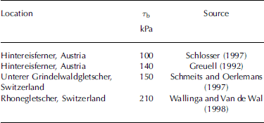
Based on historical data from Rhonegletscher, Switzerland, Reference Haeberli and SchweizerHaeberli and Schweizer (1988) calculated a basal shear stress distribution and concluded that stresses must generally be higher in steep parts than in flat parts. Hence, the constant T _b assumption is problematic (Reference Schmeits and OerlemansSchmeits and Oerlemans, 1997).

Considering these results, a more realistic approach is to find the minimum spatial variance of T _b and consequently for the interpolation value ι in an optimization process. The crucial optimization parameter is the horizontal averaging distance for the surface slope ≈. The optimum horizontal averaging distance for the surface slope α is achieved if the spatial variance of the interpolation value ι is a minimum. The optimum horizontal averaging distance itself is not quantified in this study.

Reference BindschadlerBindschadler (1982) determined a horizontal averaging distance of 8–16 times the ice thickness. Small alpine glaciers show high spatial variability of ice depths. As mentioned above, the maximum ice depth of each of the two glaciers is >100 m. Assuming a 100m ice thickness, a horizontal averaging distance of at least 800–1600m would be necessary, which seems too much for such small glaciers. This is further considered in section 7.

Variogram analysis yielded the optimum interpolation values

for PP1 (n = 1799; Fig. 4) and PP2 (n = 2033). t _0,i are the picked bedrock reflection times, and α _opt, i denotes the corresponding optimum averaged surface slopes. The optimum interpolation values ι _opt, i for PP1 and PP2 are characterized by low spatial variance, hence high spatial correlation. Optimum interpolation values l _opt, i are now interpolated using the universal kriging technique to obtain a continuous field l _opt for PP1 and PP2. A spherical variogram model was applied for universal kriging. In the case of PP1, a range of 300 m and a sill of 420 rad²˙ ns²˙ were used as variogram model parameters. Similar values were used for PP2.

Fig. 4.

Three characteristic variograms of interpolation values l _mean, i, li and l _opt, i for area PP1 (n = 1799). l _mean, i is calculated by the product of picked bedrock reflection times t _0, i and the mean surface slope α _mean of PP1. The variograms illustrate the optimization progress of averaging horizontal surface slopes. The variogram of l _opt, i values features low variance and high spatial correlation.

Finally, the interpolated continuous bedrock reflection time field l _opt for PP1 and PP2 was obtained by dividing the interpolated field I _opt by the corresponding continuous optimum averaged surface slope field A _opt:

The T _opt,PP1 kriging error shows a maximum of 213 ns (±34 m) situated at interpolated maximum bedrock reflection times, and a mean kriging error of 56 ns (±9 m). The maximum kriging error of T _opt,PP2, also situated at the interpolated maximum bedrock reflection times, is 225 ns (±36 m). The mean kriging error of T _opt,PP2 is 69 ns (±11 m; Fig. 3). For the kriging-error depth conversion, a determined propagation velocity of 0.16 mns^–1 was applied.

How the estimated picking error of IC 1 and IC 2 influences the mean kriging error was considered using the variogram parameter nugget. The nugget tests showed no significant change in the mean kriging error of PP1 and PP2.

The same interpolation steps were performed for l _mean, i to produce T _mean of PP1 (Fig. 4) and PP2. Interpolation value l _mean,i is the product of picked bedrock reflection times t _{0, i} and mean surface slope α _mean. Interpolation values l _mean,i can also be considered as picked bedrock reflection times t _{0, i} scaled by constant value α _mean. Geostatistical characteristics of l _mean,i , irrespective of the constant scaling factor α _mean, are the same as for t _{0, i} . Thus kriging errors of T _mean or interpolated t _{0, i} values are the same. Apart from resulting in implausible bedrock reflection time fields T _mean,PP1 and T _mean,PP2, a mean kriging error of 70 ns (±11 m) for PP1, and 156 ns (±25 m) for PP2, was calculated. Maximum kriging errors were of similar magnitude to those before (T _opt,PP1, T _opt,PP2).

Regarding plausible data distribution of T _opt,PP1 and T _opt,PP2, and corresponding relatively small mean kriging errors, l _opt,i prove to be appropriate interpolation values. T _opt,PP1 and T _opt,PP2 are now ready for migration.

5. 3-D Migration

The simple time-to-depth conversion,

where d is the reflector depth, t ₀ the bedrock reflection time and v _medium the propagation velocity of the medium, is only valid for horizontal or deep reflectors. In the case of alpine valley glaciers, one can expect a U-shaped glacier bed. Therefore, the correct imaging of the bed requires migration techniques (Reference Blindow, and ThyssenBlindow and Thyssen, 1986; Reference Fountain and JacobelFountain and Jacobel, 1997;Reference Welch, Pfeffer, Harper and HumphreyWelch and others, 1998; Reference Moran, Greenfield, Arcone and DelaneyMoran and others, 2000).

Migration moves dipping reflections to their true subsurface position and collapses diffraction hyperbolas, thus increasing spatial resolution and yielding a more accurate image of the subsurface (Reference YilmazYilmaz, 2001). To carry out migration, the velocity distribution of the subsurface must be known. Considering the disappearing firn coverage of the two investigated glaciers, we made a simplifying constant-propagation-velocity assumption. Following results of diffraction hyperbola analyses (Fig. 2b), a mean GPR velocity of 0.16mns^–1±5% was determined for the two investigated temperate glaciers.

2-D migration techniques assume that all reflections originate in the vertical profile plane. Considering the complex 3-D subsurface of an alpine valley glacier, these assumptions are far from reality. For a 3-D wavefield migration, optimum survey geometry is necessary (Reference Welch, Pfeffer, Harper and HumphreyWelch and others, 1998; Reference Moran, Greenfield, Arcone and DelaneyMoran and others, 2000). In this study it was not possible to produce such a dense network, due to economic and time constraints. Thus an alternative 3-D migration based on ray theory was applied.

The Eikonal equation

is a ray-theoretical approximation of the scalar wave equation (Reference YilmazYilmaz, 2001). While the solution of the scalar wave equation describes a wavefield P(x,y,z,t) at one point (x,y,z) at time t, the Eikonal equation describes the travel time T(x,y,z) for one ray in a medium with a propagation velocity v. T(x,y,z) = constant represents a wave front at time t. A wave propagates from one wave front to the next on the ray paths described by the Eikonal equation such that ray paths are normal to the propagating wave front.

The ray approximation is valid if the wavelength λ is small compared to the size of velocity anomalies in the investigated medium. Considering the boundary conditions of this 20MHz GPR survey constant mean GPR propagation velocity equal to 0.16 mns^–1±5% maximum ice thickness > 100m the Eikonal equation is a valid approximation of the scalar wave equation, and the ray approximation is well suited for this GPR survey.

Based on the Eikonal equation, a 3-D migration routine was written in Matlab programming language. To obtain the bedrock elevations (m a.s.l.) the interpolated continuous bedrock reflection time fields for PP1 and PP2 were 3-D migrated and converted to depth (Fig. 5).

Fig. 5.

Interpolated continuous bedrock reflection time fields for PP1 and PP2. Universal kriging was used for interpolation based on a spherical variogram model.

6. Final Construction of the Bedrock

In constructing the final bedrock map, we took into account the recent geomorphological history of the immediate surroundings of an alpine glacier. Apart from small-scale glacier advances (e.g. 1930), Austrian glaciers have been retreating continuously since the end of the Little Ice Age (±1850) (Reference GrossGross, 1987; Reference Lambrecht and KuhnLambrecht and Kuhn, 2007). The footprint of glacial erosion differs completely from all other exogenous processes. Given that even in areas that have been ice-free for 10 000 years, it is possible to identify glacial footprints, one can envision how long the other exogenous processes take to redesign the landscape. The immediate current surroundings of a glacier are therefore themselves part of the former glacier bedrock, so no sharp geomorphologic contrast is to be expected.

The DTM calculated from the aerial survey in 1998 delivers good data resolution of 10 m×10m of the study site (Reference Auer, Böhm, Schöner and LeymüllerAuer and others, 2002). To accomplish a realistic smooth intersection between the DTM data and the calculated bedrock of the two glaciers, we used a geomorphologic interpolation approach. As a first step we defined the footprinted area of each glacier, cut out the glaciers and trimmed the marginal region of the calculated bedrock. After merging of the masked footprinted area with the trimmed calculated bedrock (Fig. 6), the data gap between them was filled using robust nearest-neighbour interpolation (Fig. 7).

Fig. 6.

Masked DTM data merged with trimmed calculated bedrock elevations for PP1 and PP2. The geomorphologic interpolation approach satisfies a reasonably smooth intersection between the immediate surrounding and the calculated data (see Fig. 7).

Fig. 7.

Contour plot showing the calculated bedrock merged with DTM data. Greyscale plot shows the ice thickness. The data holes in PP1 are caused by rocky islands inside the glacier border. PP1, especially the Kleinfleisskees (Flk), has a classic cirque shape, while PP2 shows a more complex subglacial geometry.

7. Results and Discussion

The calculated total ice volume for PP1 (Flk and Gok 1) is 0.053±0.011km³. The calculated maximum ice thickness in the flat central part of Kleinfleisskees (Flk) is 153±34 m, and the mean ice thickness is 42 ±9 m. For PP2 (Gok 2) the calculations give a total ice volume of 0.050±0.011 km³. The calculated maximum ice thickness in the upper part of PP2 is 162±36 m, and the mean ice thickness is 48±11 m. Prior to this study, maximum ice thickness had been expected to be about 70 m, so these were surprising results.

Mean and maximum ice thickness had been adjusted by calculated elevation differences for DTM 1998 and snow cover of spring 2004. The results of testing different nugget values, according to the two picking errors of IC 1 and IC 2 data (see section 4), implied that the interpolation processing step is the main error source. The mean kriging errors were applied as total errors of mean and maximum ice thickness; total error of volume was derived by error propagation. The error of total ice volume (±±20%) is relatively large, but since interpolation is the main error source, accuracy can only be improved by densification of data coverage. Nevertheless, kriging interpolation of the optimum alternative interpolation values l _opt,i delivered reasonable data distribution. Generally, calculated maximum ice thicknesses are found in the flat parts of the two glaciers, and calculated minimum ice thicknesses in the steeper parts. Furthermore, minimum ice thicknesses correlate with the occurrence of crevasse zones, as derived from aerial survey photos, and increased reflectivity in GPR data.

Here we compare simple estimates for ice thickness and total glacier ice volume with our calculated data. Based on the constant basal shear stress assumption for steady-state glaciers and the approximation that ice is a perfectly plastic material, with a yield stress of 100 kPa (Reference PatersonPaterson, 1994; Reference SchlosserSchlosser, 1997), ice thickness can be estimated using

where H is the resulting ice-thickness field, T ₀ the yield stress (100 kPa), f a shape factor which accounts for drag on the valley side-walls and glacier bed (Reference NyeNye, 1965), ρ the ice density (900 kgm^–3), g the acceleration due to gravity (9.81ms^–2˙ ) and A _opt the corresponding optimum averaged surface slope field. Ice thicknesses calculated using this approach were compared with those produced in this study. Regression analyses were carried out and showed high correlation for PP1 (R ²˙ = 0.84) and much lower correlation for PP2 (R ²˙ = 0.49). This lower correlation is explained by the much more complex subglacial geometry that makes the constant basal shear stress assumption problematic.

Since there are volume–area scaling relations, one can calculate total glacier ice volume using a power law,

where V denotes total ice volume in km³, S the surface of the glacier in km²˙ and γ the volume–area scaling exponent. Reference Bahr, Meier and PeckhamBahr and others (1997) predict a volume–area scaling exponent γ of 1.375 for valley glaciers. Calculating total ice volumes for the two processing parts gives 1.37 km³ for PP1 and 1.06 km³ for PP2, values far different from the calculated total ice volumes. These results suggest that common volume–area scaling methods are unsuitable for small (<2 km²˙), retreating alpine valley glaciers. The relationships between characteristic quantities are typically given by power laws (Reference Schmidt and Housen.Schmidt and Housen, 1995). Besides volume–area scaling, Reference BahrBahr (1997) statistically derived other power laws relating glacier characteristics, but, like the volume–area scaling relation, the derived relationships were unsatisfactory in our case. Statistically determined characteristic values for alpine glaciers from Reference BahrBahr (1997) are very different to characteristic values for the two investigated glaciers. The fact that the study objects are small and retreating alpine glaciers, and the lack of a glacier tongue migrating into a U-shaped valley, could be explanations of this inconsistency.

The crucial parameter of the horizontal averaging distance for the surface slope to minimize the spatial variance of the derived interpolation value leaves some open questions. For an ice depth of 100 m, Reference BindschadlerBindschadler (1982) recommended a horizontal averaging distance of 800–1600 m. This seems to be far too high for the two investigated glaciers. If we take the calculated mean ice thicknesses with respect to their error margins, we obtain a recommended horizontal averaging distance of 264–816mfor PP1 and 296–944mfor PP2. These distances seem to fit better. To make a reliable statement concerning the horizontal averaging distances of small alpine valley glaciers, more data analysis and data of other comparable glaciers are required. In future work, it would be interesting to address this open question, and furthermore to quantify the absolute error of calculated bedrock topography also involving the 3-D migration processing step. A synthetic data experiment might lead to a proper error analysis. Finding possible reasons for the inconsistency of power-law relationships for characteristic values of glaciers will require data of more comparable small, retreating alpine glaciers, to determine reliable exponents. A field resurvey to collect ground truth for validation of calculated bedrock maps, ideally by means of drilling or else through GPR or seismic investigations, is also desirable.

8. Conclusion

The aim of this study was to produce bedrock topography, ice-thickness maps and consequently total ice volume based on GPR data, for two small (<2km²˙), temperate alpine glaciers. When dealing with spatially irregular and sparse data distribution, standard interpolation approaches failed. Thus the main focus of this study was to develop an appropriate interpolation technique. Eventually, the kriging technique and a glacial mechanically based interpolation parameter were used, producing reasonable bedrock topography in short CPU time. Geophysical investigations of small, remote glaciers often have to deal with rough terrain conditions and poor logistic support, due to financial constraints. Hence irregular and sparse datasets are frequent in this type of investigation area. The interpolation approach developed in this study provides an opportunity to yield objective, repeatable and comparable bedrock topographies based on further described datasets. Generally, this interpolation approach can be applied for all zero-offset data (GPR, seismics) and, furthermore, for ice-thickness interpolation itself, using the product of ice thickness h and the sine of surface slope α as an alternative interpolation value.

Considering that standard volume–area scaling methods are unsuitable for small-scale glaciers, total glacier ice volumes calculated with the presented interpolation approach could be the basis for a proper alpine glacier volume–area scaling method, for better estimating parameters such as the extent of sea-level rise caused by alpine glacier retreat.

Besides interpolation challenges presented by small glaciers, the presented interpolation approach can also be applied to larger glaciers flowing over complex bedrock topography. Derived continuous bedrock and ice-thickness maps can also be used to model glacier dynamics.