2.1 Nonlinear kinematics

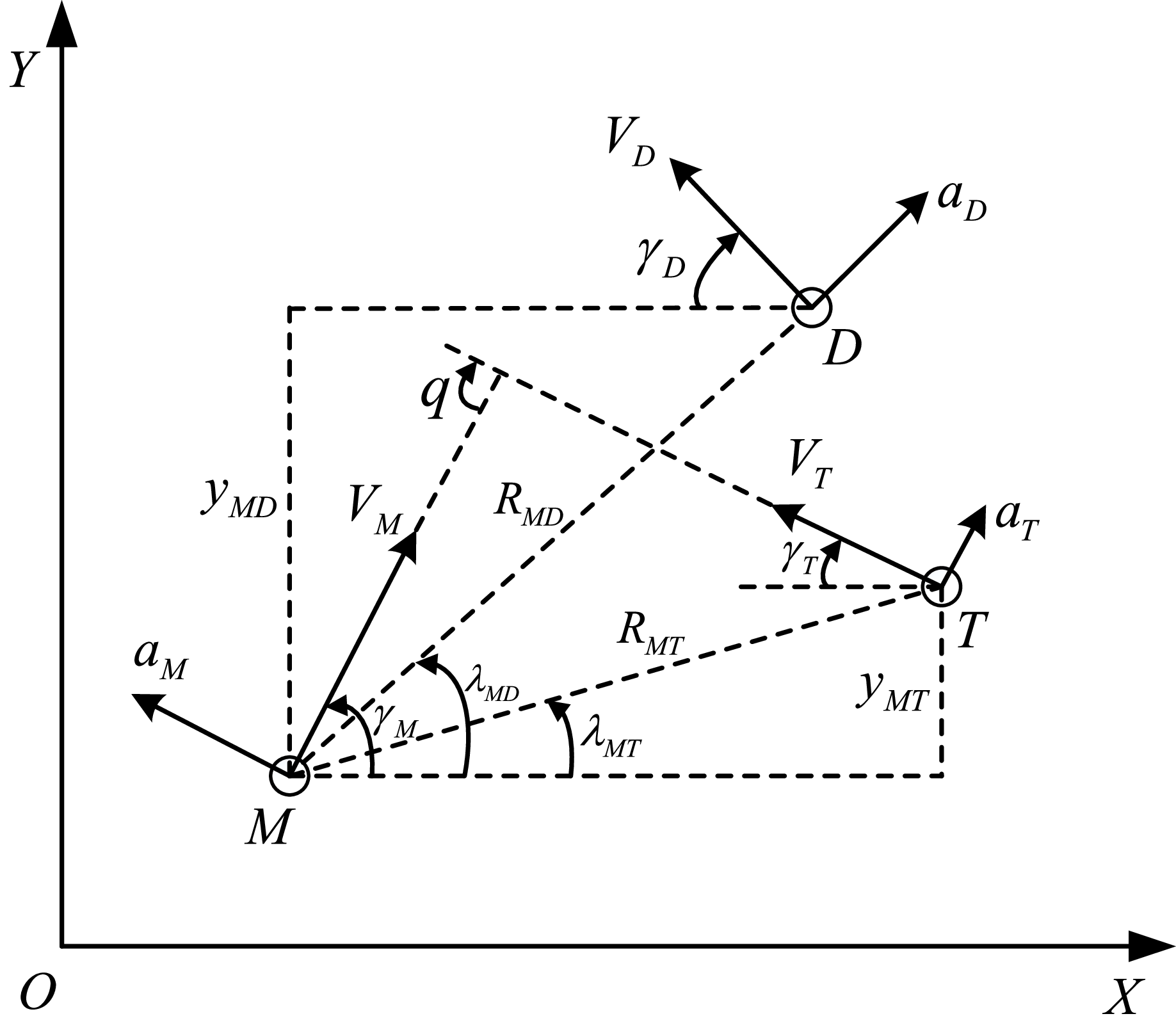
The two-dimensional engagement geometry between the three players is presented in Fig. 1, where ${R_{MT}}$ and ${R_{MD}}$ , respectively, represent the relative distances between the players. The ordinates of relative distances between the players are denoted by ${y_{MT}}$ and ${y_{MD}}$ , respectively. The velocities and accelerations of the players are represented by ${V_M}$ , ${V_T}$ , ${V_D}$ and ${a_M}$ , ${a_T}$ , ${a_D}$ , respectively. It is assumed that ${V_M}$ , ${V_T}$ and ${V_D}$ are constant, therefore ${a_M}$ , ${a_T}$ and ${a_D}$ are respectively perpendicular to ${V_M}$ , ${V_T}$ and ${V_D}$ . The line-of-sight angles between the players are denoted by ${\lambda _{MT}}$ and ${\lambda _{MD}}$ , respectively. The flight path angles of the players are respectively denoted by ${\gamma _M}$ , ${\gamma _T}$ and ${\gamma _D}$ . The angle between the velocity vectors of the missile and the target is denoted by $q$ . The desired terminal angle is denoted by ${q_f}$ . Nonlinear kinematics equations between the players can be given as follows

(1) \begin{align}{\dot R_{MT}} = - {V_M}\cos ({\gamma _M} - {\lambda _{MT}}) - {V_T}\cos ({\gamma _T} + {\lambda _{MT}}), \end{align}

(2) \begin{align}{\dot y_{MT}} = - {V_M}\sin {\gamma _M} - {V_T}\sin {\gamma _T},\end{align}

(3) \begin{align}{\dot \lambda _{MT}} = \frac{{ - {V_M}\cos ({\gamma _M} - {\lambda _{MT}}) + {V_T}\cos ({\gamma _T} + {\lambda _{MT}})}}{{{R_{MT}}}},\end{align}

(4) \begin{align}{\dot R_{MD}} = - {V_M}\cos ({\gamma _M} - {\lambda _{MD}}) - {V_D}\cos ({\gamma _D} + {\lambda _{MD}}),\end{align}

(5) \begin{align}{\dot y_{MD}} = - {V_M}\sin {\gamma _M} - {V_D}\sin {\gamma _D},\end{align}

(6) \begin{align}{\dot \lambda _{MD}} = \frac{{ - {V_M}\cos ({\gamma _M} - {\lambda _{MD}}) + {V_D}\cos ({\gamma _D} + {\lambda _{MD}})}}{{{R_{MD}}}},\end{align}

(7) \begin{align}{\dot \gamma _i} = \frac{{{a_i}}}{{{V_i}}},{\rm{ }}i = \left\{ {M,T,D} \right\},\end{align}

(8) \begin{align}\dot q = \frac{{{a_M}}}{{{V_M}}} + \frac{{{a_T}}}{{{V_T}}}.\end{align}

Figure 1.

Two-dimensional guidance geometry.

Neglecting the dynamic characteristics of the players’ autopilots, we have

(9) \begin{align}{u_i} = {a_i},{\rm{ }}i = \left\{ {M,T,D} \right\},\end{align}

where ${u_i}$ represents the guidance law of each player satisfying $\left| {{u_i}} \right| \le {\bar u_i}$ , with ${\bar u_i}$ being a positive constant representing the bound of each player’s manoeuvering capability. During the terminal guidance, the fight times are usually short and the magnitude of acceleration in time histories is small. Thus, the speeds of the players change slightly. To simplify the problem, it is assumed that the speeds of the players are constant. So, the maximum accelerations of the players are assumed constant.

In this paper, guidance laws are designed in a typical engagement [Reference Zarchan41], where a missile intercepts the target aircraft and the aircraft launches a defender to intercept the missile. Considering the engagement of the missile attacking the target and the defender intercepting the missile, the acceleration bounds of the missile and the defender are relatively large, whereas the acceleration bound of the target aircraft is relatively small, considering the structural strength of the aircraft and the tolerance of the pilots.

2.2 Nonlinear kinematics

Assume that the flight path angles and the line-of-sight angles of the players are small during the engagement, which is a common assumption in literature [Reference Perelman and Shima22]. So, it is reasonable to linearise the kinematics equations, and the state variables are defined as

(10) \begin{align}x = {\left[ {{y_{MT}}\,{{\dot y}_{MT}}\,{y_{MD}}\,{{\dot y}_{MD}}\,q - {q_f}} \right]^T},\end{align}

and the linearised kinematics equations can be given by

(11) \begin{align}\left\{ \begin{array}{l}{{\dot x}_1} = {x_2}\\{{\dot x}_2} = - {u_M} + {u_T}\\{{\dot x}_3} = {x_4}\\{{\dot x}_4} = - {u_M} + {u_D}\\{{\dot x}_5} = \frac{{{u_M}}}{{{V_M}}} + \frac{{{u_T}}}{{{V_T}}}\end{array} \right..\end{align}

Equation (11) can be written as

(12) \begin{align}\dot x = Ax + B{u_M} + C{\left[ {{u_D} \quad\!\! {u_T}} \right]^T},\end{align}

where

(13) \begin{align}A = \left[ {\begin{array}{c@{\quad}c@{\quad}c@{\quad}c@{\quad}c}0& {}1& {}0& {}0& {}0\\0& {}0& {}0& {}0& {}0\\0& {}0& {}0& {}1& {}0\\0& {}0& {}0& {}0& {}0\\0& {}0& {}0& {}0& {}0\end{array}} \right],\end{align}

(14) \begin{align}B = {\left[ {\begin{array}{c@{\quad}c@{\quad}c@{\quad}c@{\quad}c@{\quad}}0 &{ - 1} &0 &{ - 1}& {1/{V_M}}\end{array}} \right]^T},\end{align}

(15) \begin{align}C = {\left[ {\begin{array}{c@{\quad}c@{\quad}c@{\quad}c@{\quad}c}0& {}1& {}0& {}0& {}{1/{V_T}}\\0& {}0& {}0& {}1& {}0\end{array}} \right]^T}.\end{align}

3.1 Order reduction

Zero effort miss and zero effort angle, which respectively represent the miss distance and the error of intercept angle if none of the players will apply any manoeuvers, are introduced to reduce the order of the problem. Zero effort misses between the missile and the target, the missile and the defender, and the zero effort angle between the missile and the target are represented by ${Z_{MT}}$ , ${Z_{MD}}$ and ${Z_A}$ , respectively. They can be calculated by transformation [Reference Li, Yan and Gao42] as

(16) \begin{align}{Z_{MT}}(t) = {D_{MT}}\Phi ({t_{go1}})x(t),\end{align}

(17) \begin{align}{Z_{MD}}(t) = {D_{MD}}\Phi ({t_{go2}})x(t),\end{align}

(18) \begin{align}{Z_A}(t) = {D_A}\Phi ({t_{go1}})x(t),\end{align}

where ${t_{go1}}$ and ${t_{go2}}$ respectively represent the time-to-go in missile-target engagement and missile-defender engagement. ${D_{MT}}$ , ${D_{MD}}$ and ${D_A}$ are constant vectors as follows

(19) \begin{align}{D_{MT}} = {\left[ {\begin{array}{l@{\quad}l@{\quad}l@{\quad}l@{\quad}l}1 & 0 & 0 & 0 & 0\end{array}} \right]^T},\end{align}

(20) \begin{align}{D_{MD}} = {\left[ {\begin{array}{l@{\quad}l@{\quad}l@{\quad}l@{\quad}l} 0 &0 &1 &0 &0\end{array}} \right]^T},\end{align}

(21) \begin{align}\,\,\,{D_A} = {\left[ {\begin{array}{l@{\quad}l@{\quad}l@{\quad}l@{\quad}l}0 & 0 & 0 & 0 & 1 \end{array}} \right]^T}.\end{align}

$\Phi $ is the state transition matrix, which is given as

(22) \begin{align}\Phi = {L^{ - 1}}{\left[ {{{(sI - A)}^{ - 1}}} \right]^T},\end{align}

where ${L^{ - 1}}$ represents the inverse Laplace transformation and ${\rm I}$ represents the identity matrix. Thus, ${Z_{MT}}$ , ${Z_{MD}}$ and ${Z_A}$ can be given by

(23) \begin{align}{Z_{MT}} = {x_1} + {x_2}{t_{go1}},\end{align}

(24) \begin{align}{Z_{MD}} = {x_3} + {x_4}{t_{go2}},\end{align}

(25) \begin{align}{Z_A} = {x_5}.\end{align}

The derivatives of ${Z_{MT}}$ , ${Z_{MD}}$ and ${Z_A}$ can be given by

(26) \begin{align}{\dot Z_{MT}} = ( \!- {u_M} + {u_T}){t_{go1}},\end{align}

(27) \begin{align}{\dot Z_{MD}} = ( \!- {u_M} + {u_D}){t_{go2}},\end{align}

(28) \begin{align}{\dot Z_A} = \frac{{{u_M}}}{{{V_M}}} + \frac{{{u_T}}}{{{V_T}}}.\end{align}

So far, we have obtained the order-reduced model. The three players are divided into two teams. The missile is on the first team, and the second team consists of the defender and the target. The missile is required to consider both miss distances and terminal angle while the defender and the target only need to consider miss distances. Thus, the engagement in this article can be regarded as a two-team nonzero-sum game. In the following part, we will present the guidance laws of all players by solving the equilibrium solutions of the game.

3.2 Guidance law of the missile

The objective of the missile is to intercept the target while evading the defender. The guidance law is divided into two phases by the relative distance between the missile and the defender. When ${R_{MD}} \gt {\eta _1}$ ( ${\eta _1}$ is a positive constant safety distance and is taken as the switching condition of the two phases of the missile’s guidance law), it adopts the strategy of attacking the target and when ${R_{MD}} \le {\eta _1}$ , it takes the strategy of evading the defender.

Firstly, we consider the condition of ${R_{MD}} \gt {\eta _1}$ . The missile aims to attack the target, and the cost function is chosen as

(29) \begin{align}{J_1} = \frac{{{\alpha _{MT}}}}{2}Z_{MT}^2({t_{f1}}) + \frac{\beta }{2}Z_A^2({t_{f1}}) + \frac{1}{2}\int_0^{{t_{f1}}} {(u_M^2 - \eta u_T^2)} dt,\end{align}

where ${\alpha _{MT}}$ , $\beta $ and $\eta $ are weight parameters, ${t_{f1}}$ represents the interception time between the missile and the target. The Hamiltonian function is presented by

(30) \begin{align}{H_1} = {\lambda _1}{\dot Z_{MT}} + {\lambda _2}{\dot Z_A} + \frac{1}{2}u_M^2 - \frac{1}{2}\eta u_T^2.\end{align}

The adjoint variables and terminal conditions can be calculated by

(31) \begin{align}\left\{ \begin{array}{l}{{\dot \lambda }_1} = - \dfrac{{\partial {H_1}}}{{\partial {Z_{MT}}}} = 0\\[7pt]{{\dot \lambda }_2} = - \dfrac{{\partial {H_1}}}{{\partial {Z_A}}} = 0\end{array} \right.,\end{align}

(32) \begin{align}\left\{ \begin{array}{l}{\lambda _1}({t_{f1}}) = {\alpha _{MT}}{Z_{MT}}({t_{f1}})\\[5pt]{\lambda _2}({t_{f1}}) = \beta {Z_A}({t_{f1}})\end{array} \right..\end{align}

According to Equations (26) and (28), the Hamiltonian function can be rewritten as

(33) \begin{align}{H_1} = {\lambda _1}(\! - {u_M} + {u_T}){t_{go1}} + {\lambda _2}\left(\frac{{{u_M}}}{{{V_M}}} + \frac{{{u_T}}}{{{V_T}}}\right) + \frac{1}{2}u_M^2 - \frac{1}{2}\eta u_T^2.\end{align}

The guidance laws of the missile and the target given by the saddle point of the cost function Equation (29) satisfy

\begin{align*} u_M^ * = {\arg _{{u_M}}}\min {H_1},\,\,u_T^ * = {\arg _{{u_T}}}\max {H_1}. \end{align*}

According to the maximal principle [Reference Tan, Fonod and Shima43], the following equations can be obtained.

(34) \begin{align}\left\{ \begin{array}{l}\dfrac{{\partial {H_1}}}{{\partial u_M^ * }} = 0\\[8pt]\dfrac{{\partial {H_1}}}{{\partial u_T^ * }} = 0\end{array} \right..\end{align}

Accordingly, $u_M^ * $ and $u_T^ * $ can be calculated by

(35) \begin{align}\left\{ \begin{array}{l}u_M^ * = {\lambda _1}{t_{go1}} - \dfrac{{{\lambda _2}}}{{{V_M}}}\\[5pt]u_T^ * = \dfrac{1}{\eta }({\lambda _1}{t_{go1}} + \dfrac{{{\lambda _2}}}{{{V_T}}})\end{array} \right..\end{align}

Substituting Equation (32) into Equation (35), we have

(36) \begin{align}\left\{ \begin{array}{l}u_M^ * = {\alpha _{MT}}{Z_{MT}}({t_{f1}}){t_{go1}} - \dfrac{{\beta {Z_A}({t_{f1}})}}{{{V_M}}}\\[8pt]u_T^ * = \dfrac{1}{\eta }\left( {{\alpha _{MT}}{Z_{MT}}({t_{f1}}){t_{go1}} + \dfrac{{\beta {Z_A}({t_{f1}})}}{{{V_T}}}} \right)\end{array} \right..\end{align}

So far, we have obtained the open-loop solution of the differential game. Next, we will solve the state variables at the final moment, i.e., ${Z_{MT}}({t_{f1}})$ and ${Z_A}({t_{f1}})$ to get the closed-loop solution. According to Equations (26) and (28), we have

(37) \begin{align}\left\{ \begin{array}{l}{Z_{MT}}({t_{f1}}) = \int_t^{{t_{f1}}} {(\! - {u_M} + {u_T}){t_{go1}}dt} \\[6pt]{Z_A}({t_{f1}}) = \int_t^{{t_{f1}}} {\left(\frac{{{u_M}}}{{{V_M}}} + \frac{{{u_T}}}{{{V_T}}}\right)d\xi } \end{array} \right..\end{align}

Substituting Equation (36) into Equation (37) and after calculating, we have

(38) \begin{align}\left\{ \begin{array}{l}{Z_{MT}}({t_{f1}}) = \dfrac{1}{3}(\frac{1}{\eta } - 1){\alpha _{MT}}{Z_{MT}}({t_{f1}})t_{go1}^3 + \dfrac{1}{2}\left(\dfrac{1}{{\eta {V_T}}} + \frac{1}{{{V_M}}}\right)\beta {Z_A}({t_{f1}})t_{go1}^2\\[7pt]{Z_A}({t_{f1}}) = \dfrac{1}{2}\left(\dfrac{1}{{\eta {V_T}}} + \dfrac{1}{{{V_M}}}\right){\alpha _{MT}}{Z_{MT}}({t_{f1}})t_{go1}^2 + \left(\dfrac{1}{{\eta V_T^2}} - \dfrac{1}{{V_M^2}}\right)\beta {Z_A}({t_{f1}}){t_{go1}}\end{array} \right..\end{align}

By solving Equation (38), ${Z_{MT}}({t_{f1}})$ and ${Z_A}({t_{f1}})$ can be obtained. Substituting them into Equation (35), the closed-loop solution of the differential game can be obtained as follows

(39) \begin{align}\left\{ \begin{array}{l}u_M^ * = {\alpha _{MT}}{t_{go1}}{Z_{MT}}({t_{f1}}) - \dfrac{\beta }{{{V_M}}}{Z_A}({t_{f1}})\\[8pt]u_T^ * = \dfrac{1}{\eta }[{\alpha _{MT}}{t_{go1}}{Z_{MT}}({t_{f1}}) + \dfrac{\beta }{{{V_T}}}{Z_A}({t_{f1}})]\end{array} \right.,\end{align}

where ${Z_{MT}}({t_{f1}})$ and ${Z_A}({t_{f1}})$ are the solutions of Equation (38), i.e.,

(40) \begin{align}\left[ {\begin{array}{*{20}{c}}{{Z_{MT}}({t_f})}\\[8pt]{{Z_A}({t_f})}\end{array}} \right] = {\left[ {\begin{array}{*{20}{c}}{1 - \dfrac{1}{3}{\alpha _{MT}}(\dfrac{1}{\eta } - 1)t_{go1}^3} {}{ - \dfrac{1}{2}\beta (\dfrac{1}{{{V_T}\eta }} + \frac{1}{{{V_M}}})t_{go1}^2}\\[8pt]{ - \dfrac{1}{2}{\alpha _{MT}}(\frac{1}{{{V_T}\eta }} + \dfrac{1}{{{V_M}}})t_{go1}^2} {}{1 + \beta (\dfrac{1}{{V_M^2}} - \dfrac{1}{{V_T^2\eta }}){t_{go1}}}\end{array}} \right]^{ - 1}}\left[ {\begin{array}{*{20}{c}}{{Z_{MT}}}\\[8pt]{{Z_A}}\end{array}} \right].\end{align}

When ${R_{MD}} \le {\eta _1}$ , the missile takes norm-bounded guidance law to evade the defender. By solving norm-bounded differential game problem, the guidance law of the missile is derived as a bang-bang type, so the performance of the missile can be improved. The norm-bounded cost function can be given by

(41) \begin{align}{J_1} = - \frac{1}{2}Z_{MD}^2({t_{f2}}),\end{align}

where ${t_{f2}}$ represents the interception time between the missile and the defender. The corresponding Hamiltonian can be given by

(42) \begin{align}{H_1} = {\lambda _3}{\dot Z_{MD}}(t).\end{align}

The adjoint variables and the terminal condition can be calculated by

(43) \begin{align}{\dot \lambda _3} = - \frac{{\partial H}}{{\partial {Z_{MD}}}} = 0\end{align}

(44) \begin{align}{\lambda _3}({t_{f2}}) = - {Z_{MD}}({t_{f2}})\end{align}

According to Equations (27), (43) and (44), Equation (42) can be written as

(45) \begin{align}{H_1} = ({u_M} - {u_D}){Z_{MD}}{t_{go2}}\end{align}

The guidance law of the missile minimizes ${H_1}$ given in Equation (45) while that of defender maximises ${H_1}$ . The guidance laws of them can be given by

(46) \begin{align}u_M^ * = - \mu {\mathop{\rm sgn}} ({Z_{MD}}){\bar u_M}\end{align}

(47) \begin{align}u_D^ * = - {\mathop{\rm sgn}} ({Z_{MD}}){\bar u_D}\end{align}

Combining Equations (39) and (46), the missile’s guidance strategy can be given by

(48) \begin{align}u_M^ * = \left\{ \begin{array}{l} - \mu {\mathop{\rm sgn}} ({Z_{MD}}){{\bar u}_M},{\rm{ }}{R_{MD}} \le {\eta _1}\\[6pt]a{t_{go1}}{Z_{MT}}({t_{f1}}) - \frac{b}{{{V_M}}}{Z_A}({t_{f1}}),{\rm{ }}{R_{MD}} \gt {\eta _1}\end{array} \right.\end{align}

where ${Z_{MT}}({t_{f1}})$ and ${Z_A}({t_{f1}})$ are given in Equation (40), $\mu $ a coefficient satisfying $0 \lt \mu \le 1$ .

(49) \begin{align}u_M^ * = - {\mathop{\rm sgn}} (f){\bar u_M}\end{align}

where

\begin{align*}f = - {\alpha _1}{Z_{MT}}{t_{go1}} + \frac{{{\alpha _2}}}{{{V_M}}}{Z_A}\end{align*}

and ${\alpha _1}$ , ${\alpha _2}$ are constant. Differentiate f, we have

(50) \begin{align}\dot f = - {\alpha _1}( \!- {u_M} + {u_T}){t_{go1}} + {\alpha _1}{Z_{MT}} + \frac{{{\alpha _2}}}{{{V_M}}}(\frac{{{u_M}}}{{{V_M}}} + \frac{{{u_T}}}{{{V_T}}})\end{align}

When ${R_{MT}}$ is small, ${Z_{MT}}$ is small. It is assumed that ${V_M}$ and ${V_T}$ are large. So, the first term in Equation (50) dominates $\dot f$ , i.e.

(51) \begin{align}\dot f \approx - {\alpha _1}( \!- {u_M} + {u_T}){t_{go1}}\end{align}

And we assume that the manoeuvering capability of the missile is much larger than that of the target. So, ${u_M}$ plays a dominant role in Equation (50). If $f \gt 0$ , $u_M^ * \lt 0$ and $\dot f \lt 0$ , so $f$ will decrease until $f \lt 0$ . And when $f \lt 0$ , $u_M^ * \gt 0$ and $\dot f \gt 0$ , so $f$ will increase until $f \gt 0$ . Therefore, when ${R_{MT}}$ is small, $f$ will frequently switch between positive and negative values, leading chattering phenomenon of the missile’s guidance law, which is not applicable in practice. Using LQDG guidance law, $u_M^ * $ will not conclude the signal function. So, the chattering phenomenon can be reduced. The analysis of the chattering phenomenon above will be verified in simulations.

(52) \begin{align}J = \frac{{{\alpha _{MT}}}}{2}Z_{MT}^2({t_{f1}}) - \frac{{{\alpha _{MT}}}}{2}Z_{MD}^2({t_{f2}}) + \frac{\beta }{2}Z_A^2({t_{f1}}) + \frac{1}{2}\int_0^{{t_{f1}}} {(u_M^2 - {\eta _T}u_T^2 - {\eta _D}u_D^2)} dt\end{align}

which is the weighted sum of ${Z_{MT}}$ , ${Z_{MD}}$ and ${Z_A}$ , together with the integration index of respective weighted efforts. The missile is required to minimise Equation (52) while the target and the defender are required to maximise it. When both the target and the defender deviate the equilibrium solutions, there exist the possibility that the cost function is smaller than the case that both the target and the defender take the equilibrium solutions as their guidance laws. To see this, noting that in Equation (52), properly enlarging ${Z_{MT}}$ and ${Z_{MD}}$ simultaneously can also make the cost function smaller. If ${Z_{MD}}$ increases more than ${Z_{MT}}$ while ${Z_{MT}}$ is large enough for the target to evade the missile, which means the missile focuses more on evading the defender than on attacking the target, the missile will fail to hit the target. Thus, the cost function Equation (52) is unreasonable. The proposed cost function of the missile in Equations (29) and (41) is divided into two phases. When ${R_{MD}} \gt {\eta _1}$ , the missile will focus on intercepting the target and when ${R_{MD}} \le {\eta _1}$ , the missile faces the risk of being hit and will focus on evading the defender. Therefore, the cost function of the missile in Equations (29) and (41) is more reasonable.

3.3 Guidance laws of the target and the defender

Different from the missile, the target and the defender only consider miss distances, without requiring to consider the intercept angle. Thus, there is no angle constraint term in the cost functions presented in this subsection. The design of the target’s and the defender’s guidance laws is also divided by the relative distance of the players. For the defender, when ${R_{MD}} \gt {\eta _1}$ , it takes the LQGD guidance law and when ${R_{MD}} \le {\eta _1}$ , it takes the NDG guidance law. For the target, when ${R_{MT}} \gt {\eta _2}$ ( ${\eta _2}$ is also a positive constant considered as the switching condition of the two phases of the target’s guidance law), it takes the LQGD guidance law and when ${R_{MT}} \le {\eta _2}$ , it takes the NDG guidance law.

When the missile is far away from the defender and the target, i.e., ${R_{MD}} \gt {\eta _1}$ and ${R_{MT}} \gt {\eta _2}$ , the linear quadratic cost function of the defender and the target is given as

(53) \begin{align}{J_2} = \frac{{{\alpha _{MT}}}}{2}Z_{MT}^2({t_{f1}}) - \frac{{{\alpha _{MD}}}}{2}Z_{MD}^2({t_{f2}}) + \frac{1}{2}\int_0^{{t_{f1}}} {(u_M^2 - {\eta _T}u_T^2 - {\eta _D}u_D^2)} dt\end{align}

The corresponding Hamiltonian function is presented by

(54) \begin{align}\begin{array}{c}{H_2} = {\lambda _4}{{\dot Z}_{MT}}({t_{f1}}) + {\lambda _5}{{\dot Z}_{MD}}({t_{f2}})\\ = {\lambda _4}( \!- {u_M} + {u_T}){t_{go1}} + {\lambda _5}( \!- {u_M} + {u_D}){t_{go2}}\end{array}\end{align}

The guidance laws given by the saddle point of the cost function Equation (53) for the players satisfy

\begin{align*} (u_T^{ * * },u_D^{ * * }) = {\arg _{({u_T},{u_D})}}\max {H_2} \end{align*}

Using the same method in Equations (34–40), the guidance laws of the target and the defender are presented by

(55) \begin{align}u_T^{ * * } = \frac{1}{{{\eta _T}}}{\alpha _{MT}}{t_{go1}}{Z_{MT}}({t_{f1}})\end{align}

(56) \begin{align}u_D^{ * * } = - \frac{1}{{{\eta _D}}}{\alpha _{MD}}{t_{go2}}{Z_{MD}}({t_{f2}})\end{align}

where ${Z_{MT}}({t_{f1}})$ and ${Z_{MD}}({t_{f2}})$ satisfy

(57) \begin{align}\left[ {\begin{array}{*{20}{c}}{{Z_{MT}}({t_{f1}})}\\[6pt]{{Z_{MD}}({t_{f2}})}\end{array}} \right] = {\left[ {\begin{array}{*{20}{c}}{1 - \dfrac{1}{3}{\alpha _{MT}}(\dfrac{1}{{{\eta _T}}} - 1)t_{go1}^3} {}{ - {\alpha _{MD}}(\dfrac{1}{3}t_{go2}^3 + \dfrac{1}{2}t_{go2}^2\Delta t)}\\[6pt]{{\alpha _{MT}}(\dfrac{1}{3}t_{go2}^3 + \dfrac{1}{2}t_{go2}^2\Delta t)} {}{1 - \dfrac{1}{3}{\alpha _{MD}}(1 - \dfrac{1}{{{\eta _D}}})t_{go1}^3}\end{array}} \right]^{ - 1}}\left[ {\begin{array}{*{20}{c}}{{Z_{MT}}}\\[6pt]{{Z_{MD}}}\end{array}} \right]\end{align}

\begin{align*} \Delta t = {t_{f1}} - {t_{f2}} \end{align*}

When ${R_{MD}} \le {\eta _1}$ , the defender takes the NDG guidance law in Equation (47) and the target still takes the LQGD guidance law in Equation (55) When ${R_{MT}} \le {\eta _2}$ , the target takes the NDG guidance law. According to the method in Equations (41– 47), the NDG guidance law of the target can be obtained as follows

(58) \begin{align}u_T^{ * * } = - {\mathop{\rm sgn}} ({Z_{MT}}){\bar u_T}\end{align}

Thus, the guidance laws of the target and the defender can be given as

(59) \begin{align}u_T^{ * * } = \left\{ \begin{array}{l} - {\mathop{\rm sgn}} ({Z_{MT}}){{\bar u}_T},{\rm{ }}{R_{MT}} \le {\eta _2}\\[5pt]\dfrac{1}{{{\eta _T}}}{\alpha _{MT}}{t_{go1}}{Z_{MT}}({t_{f1}}),{\rm{ }}{R_{MT}} \gt {\eta _2}\end{array} \right.\end{align}

(60) \begin{align}u_D^{ * * } = \left\{ \begin{array}{l} - {\mathop{\rm sgn}} ({Z_{MD}}){{\bar u}_D},{\rm{ }}{R_{MD}} \le {\eta _1}\\[5pt] - \dfrac{1}{{{\eta _D}}}{\alpha _{MD}}{Z_{MD}}({t_{f2}}){t_{go2}},{\rm{ }}{R_{MD}} \gt {\eta _1}\end{array} \right.\end{align}

where ${Z_{MT}}({t_{f1}})$ and ${Z_{MD}}({t_{f2}})$ are given in Equation (57).

So far, we have completed the design of all players’ guidance laws which are shown in Equations (48), (59) and (60). The guidance law of the missile satisfies

(61) \begin{align}{J_1}(u_M^ * ,u_T^{ * * },u_D^{ * * }) \le {J_1}({u_M},u_T^{ * * },u_D^{ * * })\end{align}

and the guidance laws of the target and the defender satisfy

(62) \begin{align}{J_2}(u_M^ * ,u_T^{ * * },u_D^{ * * }) \le {J_2}(u_M^ * ,{u_T},{u_D})\end{align}

Therefore, $(u_M^ * ,u_T^{ * * },u_D^{ * * })$ is the equilibrium solution of the three-player conflict problem.

3.4 Time-to-go estimations

Time-to-go values in missile-target engagement and missile-defender engagement can be respectively estimated by

(63) \begin{align}{t_{go1}} = - \frac{{{R_{MT}}}}{{{{\dot R}_{MT}}}}\end{align}

(64) \begin{align}{t_{go2}} = - \frac{{{R_{MD}}}}{{{{\dot R}_{MD}}}}\end{align}

and $\Delta t$ can be calculated by

(65) \begin{align}\Delta t = {t_{go1}} - {t_{go2}}\end{align}

3.5 The principles of setting switching conditions

In this subsection, the principles of setting switching conditions ${\eta _1}$ and ${\eta _2}$ are given. For the missile evading the defender, define the switching time ${t_s}$ and assume that it satisfies

(66) \begin{align}\int_{{t_s}}^{{t_{f1}}} {( \!- {{\bar u}_D} + {{\bar u}_M}){t_{go1}}} dt = {r_c}\end{align}

(67) \begin{align}{\eta _1} = ({V_M} + {V_D})({t_{f1}} - {t_s})\end{align}

where ${r_c}$ represents the killing radius of the defender. Equation (66) means that the expected miss distance, calculated with the assumption that both the missile and the defender take norm-bounded guidance laws, equals the defender’s killing radius. In the engagement, the missile needs to estimate the upper bound of the acceleration and the killing radius of the defender to determine the switching condition, i.e., to calculate the expected miss distance. For safety consideration, a larger value than the expected miss distance is taken. After calculating, ${\eta _1}$ can be given by

(68) \begin{align}{\eta _1} = ({V_M} + {V_D})\sqrt {\frac{{2{r_c}}}{{ - {{\bar u}_D} + {{\bar u}_M}}}} \end{align}

For the target, before the interception time ${t_{f1}}$ , it takes linear quadratic differential game guidance law to cooperate with the defender for the interception of the missile. After ${t_{f1}}$ , there are only two players in the engagement – the target and the missile. And the target takes norm-bounded differential game guidance law to maximise its evasion performance against the missile. Thus, the target’s switching condition satisfies

(69) \begin{align}{\eta _2} = {R_{MT}}({t_{f1}})\end{align}

4.1 Case 1: The missile has higher manoeuvering capability

4.1.1 Verification of design rationality

In this subsection, we assume that the accelerations of the missile, the target and the defender are bounded by ${\rm{400m/}}{{\rm{s}}^{\rm{2}}}$ , ${\rm{70m/}}{{\rm{s}}^{\rm{2}}}$ and ${\rm{150m/}}{{\rm{s}}^{\rm{2}}}$ , and they take the equilibrium solutions in Equations (48), (59) and (60), and as their guidance laws, respectively. The desired terminal angle is ${40^ \circ }$ and $\mu = 0.5$ . The initial flight path angle of the missile is ${0^ \circ }$ . Other parameters are chosen as follows

\begin{align*}{\alpha _{MT}} = {\alpha _{MD}} = {10^5}, \beta = {10^8}, \eta = 8,\, {\eta _T} = {\eta _D} = 3,\, {\eta _1} = 800, {\eta _2} = 400 \end{align*}

The selections of the parameters above are referenced from the literature [Reference Perelman and Shima22, Reference Shaferman and Shima31]. The trajectories of the players are presented in Fig. 2(a). The respective miss distances between the missile, the target and the missile, the defender are 4.46m and 41.64m, which means that the missile hits the target successfully and keeps a safety distance between the defender. The error of the impact angle is ${0.13^ \circ }$ . The accelerations of the players during the engagement are presented in Fig. 2(b). When the relative distances between the players are large, LQDG guidance laws are taken to save the energy consumption, so the accelerations of the players during the first half of the engagement are small. In the endgame engagement, NDG guidance laws are taken and the accelerations of the players are large to improve their performance. When the missile takes guidance law in Equation (49), the accelerations of the players are presented in Fig. 2(c). It is obtained that the acceleration of the missile oscillates severely during the endgame engagement, which verifies the analysis in Remark 2.

4.1.2 Simulations for different parameters

In this subsection, we will change some initial conditions and parameters to verify the robustness of the design and investigate their influence on the guidance performance. Simulation results for different initial flight path angles of the missile and different desired terminal angles are shown in Tables 1 and 2. It can be obtained that with different initial flight path angles or different desired terminal angles, the missile can hit the target at the desired terminal angle and keep a safety distance between the defender.

Table 1.

Simulation results for different initial flight path angles of the missile (the desired terminal angle is ${40^ \circ }$ )

Table 2.

Simulation results for different desired terminal angles (the initial flight path angle is ${0^ \circ }$ )

Simulation results for different coefficients $\mu $ are presented in Table 3. As $\mu $ increases, the missile focuses more on evading the defender and therefore the miss distance between the missile and the defender increases. When $\mu = 1$ , the missile focuses too much on evading the defender, so the missile fails to intercept the target, which verifies the analysis in Remark 1.

Table 3.

Simulation results for different $\mu $

Simulation results for different speeds of the missile are given in Table 4. As ${V_D}$ increases, the relative velocity between the missile and the defender gets larger and it is more difficult for the defender to intercept the missile, so the miss distance between the missile and the defender becomes larger. Besides, the fight time between the missile and the target becomes longer, meaning that the missile has more sufficient time to intercept the target, so the miss distance between the missile and the target gets smaller. Simulation results for different initial positions of the players are shown in Table 5. As the initial distance between the missile and the target-defender team gets larger, the fight time between the missile and the target becomes larger, leading to a smaller miss distance.

Table 4.

Simulation results for different speeds of the defender

Table 5.

Simulation results for different initial positions of the defender and the target

Figure 3.

Comparison simulations.

4.1.3 Comparison simulations

In this subsection, comparison simulations with the approach in Ref. (Reference Saurav, Kumar and Maity32) will be given to verify the superiority of the design. We assume that guidance laws of the target and the defender deviate from the equilibrium solutions. The target’s manoeuvering strategy is

\begin{align*}{u_T} = 30 \sin (\pi t/4),\end{align*}

and the defender takes proportional navigation

\begin{align*}{u_D} = 5{\dot R_{MD}}{\dot \lambda _{MD}},\end{align*}

to intercept the missile. The desired terminal angle is ${40^ \circ }$ . Other parameters are same as those in Section 4.1.1. The trajectories of the players are presented in Fig. 3(a). Zero effort misses between the players are shown in Fig. 3(b). It can be obtained that at the terminal time, ${Z_{MT}}$ is very small in the proposed approach, but it is large in the traditional method, which means that the miss distances between the missile and the target in proposed method is smaller than that in traditional approach. The values of them are 2.64m and 21.48m, respectively. Changing the missile’s initial flight path angles, the miss distances are given in Table 6. It can be obtained that when both guidance laws of the target and the defender deviate the equilibrium solutions, the missile successfully intercepts the target in the proposed method, but fails in the traditional approach because the missile’s cost function given in this paper is more reasonable, which verifies the analyses in Remark 3 and 4.

Table 6.

Comparison simulations for different initial flight path angles of the missile

4.2 Case 2: The defender has higher manoeuver capability

In this subsection, we assume that the accelerations of the missile, the target and the defender are bounded by ${\rm{400m/}}{{\rm{s}}^{\rm{2}}}$ , ${\rm{70m/}}{{\rm{s}}^{\rm{2}}}$ and ${\rm{450m/}}{{\rm{s}}^{\rm{2}}}$ , and they take the equilibrium solutions in Equations (48), (59) and (60), and as their guidance laws, respectively. The initial flight path angle of the missile is ${10^ \circ }$ and other parameters are same as those in Section 4.1.1. Figure 4(a) shows the trajectories of the players. It is observed that the defender successfully intercepts the missile, with miss distance being 4.46m. Figure 4(b) presents the accelerations of the players. Simulation results under different initial flight path angles of the missile are given in Table 7, which reflects that the defender can successfully intercept the missile when the manoeuvering capability of the defender is higher than that of the missile.

Table 7.

Simulation results for different initial flight path angles

Figure 4.

The defender has a higher manoeuvering capability.