


1. Introduction
Wind is a dominant factor influencing snow distributions within tundra, prairie, shrubland and alpine snow covers (e.g. Reference Sturm, Holmgren and ListonSturm and others, 1995). In these environments, the frequent occurrence of blowing snow leads to considerable snow redistribution, causing accumulation in the lee of ridges, topographic depressions and taller vegetation (e.g. Seligman, 1936; Reference Kuz’minKuz’min, 1963; Reference Elder, Dozier and MichaelsenElder and others, 1991; Reference Pomeroy, Gray and LandinePomeroy and others, 1993; Reference Liston and SturmListon and Sturm, 1998; Reference Sturm, Liston, Benson and HolmgrenSturm and others, 2001a, b; Reference Hiemstra, Liston and ReinersHiemstra and others, 2002; Reference Liston and SturmListon and others, 2002). As a result of wind interaction with these variable surface features, wind-redistribution processes affect snow depths over distances of tens of centimeters to hundreds of meters (Reference BlöschlBlöschl, 1999; Reference Bruland, Liston, Vonk, Sand and Killingtveit.Liston, 2004). Further, snow transport via wind enhances sublimation of wind-borne snow crystals (Reference SchmidtSchmidt, 1972; Reference TablerTabler, 1975a; Reference Liston and SturmListon and Sturm, 1998, 2002, 2004; Reference Essery, Li and PomeroyEssery and others, 1999; Reference Pomeroy and EsseryPomeroy and Essery, 1999).
Over the past few years, snow-transport models have been developed to simulate wind-related snow-redistribution processes and consequent snow-depth patterns. The models display a wide range of complexity, but, in general, they tend toward increased realism in the physical processes represented. Models capable of simulating snow depth resulting from wind-transported snow over a spatially distributed (x,y) domain – generally called three-dimensional (3-D) models – can be divided into two temporal groups: models tailored to individual storm events and models that simulate an entire snow season (and all of the individual storms making up that season). The following summary omits 1-D (vertical) point models (e.g. Reference Xiao, Bintanja, Déry, Mann and Taylor.Xiao and others, 2000), 2-D (vertical plus one horizontal dimension) models (e.g. Reference Liston, Brown and DentListon and others, 1993b; Reference King, Anderson, Vaughan, Mann, Mobbs and Vosper.King and others, 2004) and spatially distributed models running with horizontal grid increments greater than 250 m (e.g. Reference Li, Cline, Fall, Rost and NilssonLi and others, 2001; Van Reference Van Lipzig, King, Lachlan-Cope and van den Broeke.Lipzig and others, 2004).
Four models fall into the event category and generally involve the solution of complex, 3-D wind fields over high-resolution grids. (1) Reference Uematsu, Nakata, Takeuchi, Arisawa and KanedaUematsu and others (1991) and Reference Uematsu, Nakata, Takeuchi, Arisawa and KanedaUematsu (1993) developed a 3-D numerical simulation model of snow transport and drift formation, and applied it to idealized hills. (2) Reference SundsbøSundsbø (1997) developed a SNOW-SIM model and applied it to idealized block structures representing buildings. (3) Reference GauerGauer (2001) developed a physically based numerical model that includes particle-trajectory calculations in the saltation simulations, and a two-way coupling between the particles and airflow, and applied it to Gaudergrat ridge in the Swiss Alps. (4) Reference Doorschot and LehningLehning and others (2002) developed a snow-redistribution model that uses a mesoscale meteorological model to simulate the wind field; this was also tested over Gaudergrat ridge. Ultimately, this approach requires considerable computational energy for simulating the wind fields. Therefore, the models are unable to simulate snow evolution for more than a few days.
Seven models fall into the seasonal category; these are generally intermediate-complexity models that have been configured to capture first-order transport physics while still being able to simulate spatial snow distributions over the entire snow season. (1) Reference Li and PomeroyPomeroy and others (1997) divided an arctic Canada watershed into blowing-snow source and sink sub-regions based on vegetation and topography, and applied a modified version of the prairie blowing-snow model (PBSM; Reference Pomeroy, Gray and LandinePomeroy and others, 1993) to determine end- of-winter snow depths. Reference PomeroyPomeroy and others (1998), Reference Essery, Li and PomeroyEssery and others (1999) and Reference Essery and PomeroyEssery and Pomeroy (2004) used an improved version of PBSM (Reference Essery, Li and PomeroyEssery and others, 1999; Reference Pomeroy and LiPomeroy and Li, 2000) to simulate snow distributions in Canadian prairie and arctic landscapes. PBSM was the first physically based blowing-snow model and it strongly influenced many subsequent models. (2) Reference Purves, Barton, Mackaness and Sugden.Purves and others (1998) presented a rule- and cell-based wind-transport and deposition model and applied it to the western highlands of Scotland; simple rules were used to move snow from one model cell to another. (3) Taking advantage of PBSM contributions, Reference Liston and SturmListon and Sturm (1998) introduced equations that accounted for accelerating and decelerating wind-flow influences on snow erosion and deposition. The resulting numerical snow-transport model (SnowTran-3D, version 1.0) was applied in an arctic Alaska landscape. (4) Building on the work of Reference Li and PomeroyPomeroy and others (1997) and Reference Liston and SturmListon and Sturm (1998), Reference JaedickeJaedicke (2001) developed a snow-transport model and applied it to the Drønbreen area of Spitsbergen in arctic Norway. (5) Reference Winstral and MarksWinstral and Marks (2002) and Reference Winstral and MarksWinstral and others (2002) developed a series of terrain-based parameters to characterize the effects of wind on snow redistribution in Idaho and Colorado, USA. (6) Reference Durand and CorripioDurand and others (2005) implemented a snowdrift model called SYTRON3 in the SAFRAN–Crocus–MÉPRA operational snowpack and avalanche-risk forecasting modeling system. (7) Reference Lehning, Völksch, Gustafsson, Nguyen, Stähli and Zappa.Lehning and others (2006) included a snow-transport module in the ALPINE3D mountain surface-processes model.
We have had a long-term goal of developing a model that was widely applicable and useful in different environments. As part of our SnowTran-3D (version 1.0) model description (Reference Liston and SturmListon and Sturm 1998), we identified several model limitations that prevented general application to the range of snow, topographic and climatic conditions found around the world. To correct these deficiencies, three model improvements were required. First, the simple wind model needed to be modified to account for a wider range of topographic configurations. Second, the snow threshold friction velocity needed to be defined to vary spatially and temporally in response to temperature, wind transport and precipitation timing (e.g. to account for applications where relatively high air temperatures and/or wind transport produce well-bonded snow covers). Finally, the simulated snow accumulations needed to evolve with time and match observed equilibrium-drift profiles. In what follows, we describe how we made these improvements and present a version of SnowTran-3D (version 2.0) capable of simulating wind-related snow distributions over a wide range of topographic and climatic environments found globally. In addition, to complete this goal of general applicability, we summarize the coupling of SnowTran-3D with a meteorological distribution model (MicroMet; Reference Liston and ElderListon and Elder 2006b) and an energy- and mass-balance snow-evolution modeling system (SnowModel; Reference Liston and ElderListon and Elder, 2006a).
2. Snowtran-3D Model
2.1. Model description
SnowTran-3D is a 3-D model that simulates wind-driven snow-depth evolution over topographically variable terrain (Fig. 1). The model was developed and tested in an arctic–tundra landscape (Reference Liston and SturmListon and Sturm, 1998, 2002), but is generally applicable to other treeless areas characterized by strong winds, below-freezing temperatures and solid precipitation. Since its introduction, SnowTran-3D has been used over a wide variety of landscapes, including Colorado (Reference Greene, Liston and PielkeGreene and others, 1999), Antarctica (Reference Liston, Winther, Bruland, Elvehøy, Sand and Karlöf.Liston and others, 2000), Idaho (Reference Prasad, Tarboton, Liston, Luce and SeyfriedPrasad and others, 2001), Wyoming, USA (Reference Hiemstra, Liston and ReinersHiemstra and others, 2002, 2006), Alaska (Reference Liston and SturmListon and Sturm, 2002; Reference Liston and SturmListon and others, 2002), Greenland (Reference Hasholt, Liston and KnudsenHasholt and others, 2003; Reference Mernild, Liston, Hasholt and Knudsen.Mernild and others, 2006), Svalbard/Norway (Reference Bruland, Liston, Vonk, Sand and Killingtveit.Bruland and others, 2004), Siberia (Reference Hirashima, Ohata, Kodama, Yabuki, Sato and GeorgiadiHirashima and others, 2004) and the European Alps (Reference Bernhardt, Zälngl, Liston, Strasser and Mauser.Bernhardt and others, in press).
Key features of SnowTran-3D (following Reference Liston and SturmListon and Sturm, 1998).

SnowTran-3D’s primary components are: (1) the wind-flow forcing field, (2) the wind-shear stress on the surface, (3) the transport of snow by saltation and turbulent suspension (the dominant wind-transport modes), (4) the sublimation of saltating and suspended snow and (5) the accumulation and erosion of snow at the snow surface (Fig. 1). SnowTran-3D can be run using temporal increments ranging from 5 min to 1 day (hourly is typical), and horizontal grid increments ranging from 1 m to 1 km (although for increments greater than ~100 m the redistribution components of the model become negligible and only the simulated sublimation is significant). Required model inputs include topography, vegetation and spatially distributed, temporally variant weather data (fields of precipitation, wind speed and direction, air temperature and humidity) obtained from meteorological-station and/or atmospheric-model data located within or near the simulation domain. Within the model, each gridcell is assigned a single vegetation type, and each vegetation type is assigned a canopy height that defines the vegetation’s snow-holding depth. Snow depth must exceed the vegetation snowholding depth before snow becomes available for wind transport (i.e. snow captured within the vegetation canopy by either precipitation or blowing-snow deposition cannot be removed by the wind). Because of important snow–vegetation interactions (Reference McFadden, Liston, Sturm, Pielke, Sr and Chapin, III.McFadden and others, 2001; Reference Sturm, Liston, Benson and HolmgrenSturm and others, 2001b; Reference Liston and SturmListon and others, 2002), SnowTran-3D simulates the snow-depth evolution. For hydrologic applications, the snow density is used to convert to snow water equivalent (SWE).
The foundation of SnowTran-3D is a mass-balance equation that describes the temporal variation of snow depth at each point within the simulation domain. Deposition and erosion, which lead to changes in snow depth at these points, result from: (1) changes in horizontal mass-transport rates of saltation, Q salt (kg m−1 s−1); (2) differences in horizontal mass-transport rates of turbulent-suspended snow, Q turb (kg m−1s−1); (3) sublimation of transported snow particles, Q v (kg m−2 s−1); and (4) the rate of water equivalent precipitation, P(m s−1). Transport in the creeping and rolling modes is assumed to be negligibly small. Combined, the time rate of change of snow depth, ζ (m), is

where t (s) is time, x (m) and y (m) are the horizontal coordinates in the west–east and south–north directions, respectively, and ρ s and ρ w (kg m−3) are the snow and water density, respectively. In this formulation, transports to the surface are defined to be positive. At each time-step, Equation (1) is solved for individual gridcells within the domain and is coupled to the neighboring cells through spatial derivatives (d/dx, d/dy).
In the Equation (1) formulation, saltation transport, Q salt, is given by Reference Pomeroy and GrayPomeroy and Gray (1990) and turbulent-suspended transport, Q turb, is given by Reference KindKind (1992) (see Reference Liston and SturmListon and Sturm, 1998). Reference Doorschot and LehningDoorschot and Lehning (2002) showed saltation mass fluxes are much greater than those given by Reference Pomeroy and GrayPomeroy and Gray (1990). In our formulation, the saltation fluxes are rapidly dominated by suspended transport for wind-shear velocities greater than 0.4 m s−1 (Reference Liston and SturmListon and Sturm, 1998), and as a consequence the combined saltation and suspended transport for our formulation is comparable to the transport defined by Reference Doorschot and LehningDoorschot and Lehning (2002). In addition, there is some debate in the literature regarding the importance of the blowing-snow sublimation term in Equation (1). A summary of the relevant issues can be found in Reference ListonListon and Sturm (2004) and references therein.
2.2. Model improvements
In the original paper describing SnowTran-3D, we cited several model-related limitations (Reference Liston and SturmListon and Sturm, 1998). While these did not appear to degrade our arctic simulations, we noted that corrections were needed to make SnowTran-3D completely general and applicable to a wider range of topographic situations and climates. The SnowTran-3D (version 2.0) improvements presented here are: (1) an improved wind model that accounts for wind speed and direction variations in variable topography, (2) a threshold-shear/friction-velocity parameterization that accounts for snow’s resistance to transport when surface temperatures are at or near freezing and (3) an equilibrium-profile sub-model that constrains the evolving drift profiles.
2.2.1. Wind model
Wind fields in topographic configurations range from simple to complex, depending on factors including feature size, orientation and slope steepness. Many models have been developed to simulate wind fields in variable topography. These range from the simple empirical model of Reference Liston and SturmListon and Sturm (1998) to complex models that solve full momentum, continuity and turbulent-transport equations for the flow field (e.g. Reference Liston, Brown and DentListon and others, 1993a; Reference CottonCotton and others, 2003). The original wind-speed model used in SnowTran-3D lacked wind speed and direction variations around large-scale topographic features. The simple wind model also did not adequately account for increased wind speeds on the tops of ridges, hills and mountains, and was unable to simulate decreased wind speed from divergent flow immediately upwind of an abrupt topographic obstruction.
To generate distributed wind fields for SnowTran-3D (version 2.0), wind speed and direction data are interpolated to the SnowTran-3D grid and adjusted for topography. Since wind-direction data are recorded in radial coordinates, station wind speed (W) and direction (θ) values are first converted to zonal, u, and meridional, v, components using


The u and v components are then independently interpolated to the model grid using the Barnes objective analysis scheme (Reference Koch and KocinKoch and others, 1983) contained within the MicroMet meteorological distribution model (Reference Liston and ElderListon and Elder, 2006b; see section 2.3 below for a summary of how SnowTran-3D and MicroMet are connected). The resulting values are converted back to speed and direction using


where north is zero.
Gridded speed and direction values are modified using a simple, topographically driven wind model following Reference Liston and SturmListon and Sturm (1998) that adjusts speeds and directions according to topographic slope and curvature relationships. Conceptually, this model identifies four classes of topographic features: convex and concave areas (i.e. areas of positive and negative curvature, respectively) and windward and leeward slopes (i.e. positive and negative slopes, respectively). For these classes, curvature and slope are computed. Positive curvature and slope have positive values, negative curvature and slope have negative values, and values increase with increasing curvature and slope and decrease with decreasing curvature and slope. The values are then used as weights to produce higher wind speeds on windward slopes and at the tops of topographic ridges and peaks, and lower wind speeds on leeward slopes and at the bottoms of topographic valleys and depressions.
To calculate the wind modifications, slope, slope azimuth and topographic curvature must be computed. The terrain slope, β, is given by

where z is the topographic height, and x and y are the horizontal coordinates. The terrain slope azimuth, ξ, with north having zero azimuth, is

Topographic curvature, Ωc, is computed at each model gridcell by first defining a curvature length scale or radius, η, which defines the length scale to be used by the curvature calculation. This length scale equals half the wavelength of topographic features relevant in snow-redistribution processes. Conceptually, it defines the distance from the top of a typical ridge that experiences erosion, to a topographic depression that receives snow. Only one time-invariant length scale is associated with the curvature calculation, and this scale must be equal to or greater than the model grid increment; the user must choose the length scale most relevant to snow-redistribution processes within their simulation domain. Reference Fels and MatsonFels and Matson (1997) describe methods to calculate topography-associated length scales.
For each model gridcell, curvature is calculated by taking the difference between that gridcell elevation and the average elevations of two opposite gridcells a length-scale distance from that gridcell. This difference is calculated for each of the opposing directions south–north, west–east, southwest–northeast and northwest–southeast from the main gridcell (effectively obtaining a curvature for each of the four direction lines), and the resulting four values are averaged to obtain the curvature. Thus,
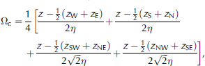
where z W, z SE, etc. are the elevation values for the gridcell at approximately curvature length scale distance, η, in the corresponding direction from the main gridcell. The curvature is then scaled such that −0.5 ≤ Ωc ≤ 0.5 (this is accomplished by dividing the calculated curvature by twice the maximum curvature found within the simulation domain). This scaling is done to allow an intuitive application of the slope and curve weight parameters, described below. The slope in the direction of the wind, Ωs, is

This Ωs is scaled in the same way as for curvature, such that −0.5 ≤ Ωs ≤ 0.5.
The wind weighting factor, W W, that is used to modify the wind speed is given by

where γ s and γ c are the slope weight and curvature weight, respectively (Reference Liston and SturmListon and Sturm, 1998). The Ωs and Ωc values range between −0.5 and +0.5. Valid γ s and γ c values are between 0 and 1, with values of 0.5 giving approximately equal weight to slope and curvature. Experience suggests that γ s and γ c be set such that γ s + γ c = 1.0, limiting the total wind weight between 0.5 and 1.5; these values produce wind fields consistent with observations of wind microtopographic relationships (Reference YoshinoYoshino, 1975; Reference Pohl, Marsh and ListonPohl and others, 2006). Finally, the terrain-modified wind speed, W t (ms−1), is calculated from

Wind directions are modified by a diverting factor, θ d, according to Reference RyanRyan (1977),

This diverting factor is added to the wind direction to yield the terrain-modified wind direction, θ t,

The resulting speeds, W t, and directions, θ t, are converted to u and v components using Equations (2) and (3) and used to drive SnowTran-3D.
2.2.2. Threshold friction velocity
In SnowTran-3D’s original low-temperature arctic application, where surface melting was minimal, it was acceptable to use a spatially and temporally constant snow density and threshold shear/friction velocity. In temperate climates, this assumption is generally inappropriate; temperatures near and above freezing can limit or stop surface snowdrifting. In addition, previously wind-transported snow is generally harder to transport. Thus, a parameterization is required that defines the evolution of the snow threshold friction velocity as a function of snow temperature, precipitation and wind-transport histories.
To account for snow surface characteristics, SnowTran-3D’s snowpack is composed of two layers, a ‘soft’ surface layer that stores mobile snow and a ‘hard’ immobile underlying layer. To determine the threshold friction velocity, u *t, of the soft snow, the temporal evolution of snow density, ρ s, is simulated and related to snow strength and hardness, which is then related to u *t.
Density changes in the soft layer occur by two mechanisms. First, snow precipitation is added to the soft layer using an air-temperature-dependent new-snow density, p ns(kg m−3), calculated following Reference AndersonAnderson (1976), based on data by Reference LaChapelleLaChapelle (1969),

where T wb is the wet-bulb air temperature (K). The wet-bulb temperature is calculated within SnowModel (Reference Liston and ElderListon and Elder, 2006a) following Reference Liston and HallListon and Hall (1995) (see section 2.3 for a summary of how SnowTran-3D and SnowModel are related).
The second mechanism increases snow density through compaction and includes the influences of air/snow temperature and wind speed (the following formulation corrects deficiencies presented in Reference Bruland, Liston, Vonk, Sand and Killingtveit.Bruland and others (2004)). During precipitation periods and wind speeds less than 5 m s−1, the temperature-dependent new-snow density, ρ ns, is used. For wind speeds ≥5 m s−1, a wind-related density offset, ρ w(kg m−3), is added to the temperature-dependent density,

with

where D1, D2 and D3 are constants set equal to 25.0 kg m−3, 250.0 kg m−3 and 0.2 m s−1, respectively; D1 defines the density offset for a 5.0 m s−1 wind, D 2 defines the maximum density increase due to wind and D3 controls the progression from low to high wind speeds. In Equation (16), the terrain-modified wind speed, W t, is assumed to be at 2 m height.
During periods of no precipitation, the soft snow density evolves in a manner similar to that defined by Reference AndersonAnderson (1976), but with a wind-speed contribution, U. The temporal change in snow density, ρ s, is given by

where T f is the freezing temperature, T s is the soft snow temperature (defined in this application to be equal to the lesser of the air temperature or the freezing temperature), B is a constant equal to 0.08 K−1, A 1 and A 2 are constants set equal to 0.0013 m−1 and 0.021m3 kg−1, respectively (Reference Kojima and OuraKojima, 1967), and C = 0.10 is a non-dimensional constant that controls the simulated snow density change rate. For wind speeds ≥5 m s−1, U is given by

with E 1, E 2 and E 3 defined to be 5.0 ms−1, 15.0 ms−1 and 0.2 m s−1, respectively; E 1 defines the U offset for a 5.0 m s−1 wind, E 2 defines the maximum U increase due to wind and E 3 controls the progression of U from low to high wind speeds. For speeds <5 m s−1, U is defined to be 1.0 m s−1. This approach limits the density increase resulting from wind transport to winds capable of moving snow (assumed to be winds ≥5 m s−1). Numerous studies have observed a 4–5 ms−1 snow-transport wind-speed threshold for new or slightly aged cold, dry (i.e. below ~−2°C) snow (see Reference Kind, Gray and Male, edsKind, 1981 and references therein; and Reference Li and PomeroyLi and Pomeroy, 1997). They also noted a clear threshold-speed dependence on environmental (e.g. temperature and wind-speed) conditions and histories (increasing threshold speed with increasing temperature, wind speed and time, which are calculated by the other components of SnowTran-3D’s two-layer submodel).
Simulated snow density is related to snow strength using the uniaxial compression measurements of Reference Abele and GowAbele and Gow (1975). An equation fitted to their results describes the variation of hardness, σ, with snow density,

where σ is in kPa, and ρ s is in kg m−3. A relationship between hardness and u *t, for snow densities of 300–450 kg m−3, is provided using the data of Reference KotlyakovKotlyakov (1961),

Combining Equations (19) and (20) yields

For snow densities of 50–300 kg m−3, a similar equation is used:

Equations (21) and (22) yield the threshold friction velocity from the computed soft snow layer density evolution defined by Equations (15–18). Ideally, Equations (15–22) are coupled and require an iterative solution (the 5 m s−1 wind-speed threshold value depends on u *t). Unfortunately, comprehensive observational datasets that would allow us to define the exact relationships between ρ s and u *t do not exist, so the relatively simple approach above is used.
Implementation of these equations in SnowTran-3D allows the threshold friction velocity of the soft snow layer to evolve throughout the model simulation. At any point in time when the snow threshold friction velocity exceeds a value for snow that cannot be transported by naturally occurring winds (e.g. u *t ≥ 1.7 ms−1, corresponding to a 10m wind speed of approximately 40 m s−1), the soft snow layer is added to the hard (unmovable) snow layer. From this point in time, any new snow, arriving from solid precipitation or other redistributed snow, rebuilds the soft snow layer and is available for wind redistribution. Conceptually, the two-layer model can be thought of as a transportable soft snow layer that is governed by the mass-balance formulation given by Equation (1), and a hard snow layer (that cannot be moved by naturally occurring winds) that sits under the soft layer (i.e. when the soft layer is eroded down to the hard layer, in any given gridcell, transport out of that gridcell stops).
Other researchers have proposed alternative methods to define threshold wind speed. For example, Reference SchmidtSchmidt (1980) developed a model relating speed threshold to cohesive bonding between ice grains. Reference Lehning, Doorschot, Fierz and RaderschallLehning and others (2000) reformulated that relationship to be a function of grain sphericity and a measure of the number of bonds per particle. Reference Clifton, Rüedi and LehningClifton and others (2006) showed that both these formulations agree well with observations. Unfortunately, models that evolve grain sphericity and bonds per particle as a function of air temperature, wind speed and history of these two physical forcing variables are still in their infancy. As an alternative, we have formulated our threshold wind speed as a function of snow density evolution, and have implemented that evolution based on generally accepted relationships between air temperature and wind speed. We recognize that factors other than density can have a large impact on threshold wind speed (e.g. depth hoar generally has minimal bonding strength relative to its density), but at this time we know of no other formulation that meets our requirements of broad applicability and computational efficiency.
Under some conditions, our use of a simple two-layer model may also oversimplify the natural system. Real snowpacks are frequently composed of a mix of relatively hard and soft layers, and the erosion of a hard layer above may expose easily transported snow below. We have avoided the complexity of keeping track of more than two layers, and thus SnowTran-3D cannot realistically handle this more complex case. Essentially we have assumed the first-order feature in this environment is that the newest snow is the most available for redistribution.
2.2.3. Drift profiles
Dramatic decreases in surface wind friction velocity occur over sharp ridge crests. This produces strong decreases in horizontal snow transport and significant accumulation in the lee of the ridge. Within a snow-transport model such as SnowTran-3D, this transport decrease and associated snow accumulation are easily simulated. Over time, however, the simulated lee-slope snow deposition could accumulate to be unrealistically higher than the elevation of the gridcell immediately upwind of the lee gridcell (Reference Liston and SturmListon and Sturm, 1998). Observations show the wind would rapidly erode and transport this snow bump downwind. Such processes cannot be directly simulated using a snow-transport model operating on relatively long (e.g. hourly) time increments. Thus, SnowTran-3D requires an additional parameterization to account for the effects of these processes. This need is most critical when the vertical scale of snow accumulation is similar to the model’s horizontal grid increment.
Reference TablerTabler (1975b) introduced the idea of an equilibrium profile for snowdrifts, and described the mechanisms by which such a profile forms. Unfortunately, little additional research has been done to expand on that early work. In an effort to quantify the relationships between terrain and snow distributions in windy environments, Tabler developed an empirical regression model that predicts 2-D (cross-section) equilibrium-snowdrift profiles based on topographic variations in the direction of wind flow. The equilibrium-snowdrift profile is the snow surface that corresponds to the maximum snow retention depth of a topographic drift trap; any additional blowing snow entering the trap is transported downwind of the trap.
To develop the regression model, Reference TablerTabler (1975b) used terrain- and snow-slope field measurements from 17 different sites in Colorado and Wyoming. Half of the available data were used to develop the regression equation, and the other half were used for testing. Tabler found the following regression equation minimized the residual variance (r 2 = 0.87):

where Y is the snow slope (%) of the drift downwind of the drift trap lip, X 0 is the average ground slope (%) over the 45 m distance upwind of the drift trap lip and X 1, X 2 and X 3 are the ground slopes (%) over distances of 0–15, 15–30 and 30–45 m downwind of the drift trap lip, respectively. Upward slopes in the direction of the wind are positive and downward slopes are negative.
Tabler noted that if Equation (23) is generally applicable to drift traps of any size or shape, it should also simulate the snow slope at any point along the drift surface. This occurs because, in the natural system, upwind drift portions tend to approach their equilibrium profile even though the downwind portion is not yet completely full. If we follow the time evolution of a drift profile, we see that the profile at a given time essentially defines the topographic configuration governing the equilibrium-drift profile at a later time. Thus, Equation (23) can be used to define the slope of successive equilibrium-drift surface elements by starting upwind of the drift trap and continuing along the wind-flow direction until the ground is intercepted. Tabler found his methodology closely simulated all the measured equilibrium-drift profiles he had available. These covered a diverse range of environments in the plains and mountains of Colorado and Wyoming. An attractive feature of this methodology is that the resulting drift profiles inherently assume the influence of naturally occurring complex wind fields found in the lee of the topographic obstructions, and the subsequent influence on the resulting snow distributions. Therefore, simulations of highly accurate lee-slope wind fields are not required.
To incorporate the Reference TablerTabler (1975b) model into SnowTran-3D, there are three requirements. It must work under any defined grid spacing, it must appropriately handle any wind direction, and subsequent wind- and snow-transport fields must adopt the underlying snow surface as the governing and time-evolving topographic surface. To satisfy the general grid spacing requirement, topographic profiles in each of the eight principal wind directions (north, northeast, east, etc.) across the entire SnowTran-3D simulation domain are extracted from topography. The profiles are each linearly interpolated to a 1 m grid and used to generate high-resolution equilibrium surface profiles. Implementing the Tabler model on this relatively fine grid is necessary to reproduce observed equilibrium-drift profiles. The Tabler model continually simulates the drift profile as the drift trap fills in response to the evolving local snow/topographic profile. The 1 m grid increment is sufficient to reproduce the evolution found in the natural system and to generate an appropriate equilibrium profile (the same profile is not generated when using significantly larger grid increments; because the model generates, uses and discards a single 1 m profile line across the simulation domain before moving on the next profile, the 1 m increment is not computationally restrictive). The 1 m gridpoints that are coincident with the SnowTran-3D topography gridpoints are then extracted and used to build equilibrium surfaces over the simulation domain at the SnowTran-3D simulation-grid resolution. The equilibrium surfaces on the model topography gridpoints are then used in the model simulations. This interpolation procedure allows SnowTran-3D to generate equilibrium-drift surfaces for any model grid increment ≥1 m.
As part of the implementation, eight different equilibrium-drift surface distributions are generated over the simulation domain corresponding to the eight primary wind directions. These are then used, in conjunction with a user-defined primary drift direction, to generate the equilibrium-drift surface that corresponds to that drift direction. The SnowTran-3D implementation also includes the ability to increase or decrease the slope of the calculated equilibrium-drift profiles by implementing a slope-adjustment scaling factor, S, for Equation (23),

where S is a non-dimensional user-defined parameter that adjusts the overall slope of the calculated drift profiles. This parameter allows the user to modify the simulated drift profiles to more closely match observational datasets and account for regional differences in equilibrium-drift slopes. For example, Reference Sturm, Liston, Benson and HolmgrenSturm and others (2001a) found drift slopes averaging 29–36% for drifts in arctic Alaska, compared with an average of 24% for drifts with similar topographic configurations in Colorado and Wyoming (Reference TablerTabler, 1975b). While we do not know the true reason for these differences, we expect they are caused by wind direction variations at the research sites (the wind flow may not always be perpendicular to the topographic break).
During a model simulation, SnowTran-3D wind directions are decomposed into x and y components and used to partition the snow-transport fluxes across the model grid (Reference Liston and SturmListon and Sturm, 1998). As part of this snow-redistribution process, any simulated snow accumulation deeper than the equilibrium-drift surface is transported downwind into the next gridcell. This process implicitly assumes that the snow surface at any given model time-step represents the ‘topography’ followed by any ensuing wind and associated snow transport.
2.3. Coupling SnowTran-3D with MicroMet and SnowModel
In the original Reference Liston and SturmListon and Sturm (1998) SnowTran-3D simulations, data from a single meteorological tower were used to force model integrations. For larger computational domains (e.g. Reference Liston and SturmListon and Sturm, 2002), multiple meteorological towers may be available to quantify local and/or regional atmospheric forcing values and gradients. To include such datasets within SnowTran-3D (version 2.0) simulations, the model uses MicroMet (Reference Liston and ElderListon and Elder, 2006b), a quasi-physically based, high-resolution (e.g. 1 m to 1 km horizontal grid increment), meteorological-distribution model. MicroMet minimally requires screen-height air temperature, relative humidity, precipitation and wind speed and direction.
MicroMet produces high-resolution meteorological forcing distributions required to run spatially distributed terrestrial models over a wide variety of landscapes. It is a data-assimilation and interpolation model that utilizes meteorological station datasets and/or gridded atmospheric-model or analyses datasets. The model uses known relationships between meteorological variables and the surrounding landscape (primarily topography) to distribute those variables over any given landscape in computationally efficient and physically plausible ways. MicroMet performs two kinds of adjustments to the meteorological data: (1) all available data, at a given time, are spatially interpolated over the domain and (2) physical sub-models are applied to each MicroMet variable to improve realism at a given point in space and time. Station interpolations (horizontal) are done using a Barnes objective analysis scheme (Reference BarnesBarnes, 1964, 1973; Reference Koch and KocinKoch and others, 1983). Objective analysis is the process of interpolating data from irregularly spaced stations to a regular grid. At each time-step, MicroMet generates distributions of air temperature, relative humidity, wind speed, wind direction, incoming solar radiation, incoming longwave radiation, surface pressure and precipitation.
SnowTran-3D is also coupled with SnowModel, an energy- and mass-balance snow-evolution system (Reference Liston and ElderListon and Elder, 2006a). SnowModel is a spatially distributed snow model designed for application in landscapes, climates and conditions where snow occurs. The model includes an energy-balance sub-model that calculates surface energy exchanges and melt, and a snowpack submodel that simulates snow depth and water-equivalent evolution. When coupled with SnowTran-3D and MicroMet, SnowModel-simulated processes include snow accumulation; blowing-snow redistribution and sublimation; forest canopy interception, unloading and sublimation; snow-density evolution and snowpack melt. Conceptually, Snow-Model includes the first-order physics required to simulate snow evolution within each of the global snow classes defined by Reference Sturm, Holmgren and ListonSturm and others (1995) (i.e. ice, tundra, taiga, alpine/mountain, prairie, maritime and ephemeral). The required model inputs are the same as those required for SnowTran-3D. An attractive feature of the distributed MicroMet/SnowModel/SnowTran-3D snow-evolution modeling system is that, for example, it can blow and drift snow in an alpine area of the simulation domain while it melts snow in a valley below.
3. Results
To test SnowTran-3D performance, we applied the model to a collection of idealized and real landscape model simulations. In what follows we use those simulations to demonstrate the utility of the wind model, threshold friction velocity and drift profile enhancements.
3.1. Wind model
Wind-model behavior is highlighted in Figure 2, where a westerly background wind of 8 m s−1 flows over a symmetric hill 50 m high with a radius of 1 km. Simulated wind fields for various slope-weight, γ s, and curvature-weight, γ c, values are shown. In this example simulation, the curvature length scale, η, was defined to be 1000 m. Using this characteristic length, the model recognizes the positive curvatures defined by the hill top, and negative curvature associated with the transition between the flat surrounding topography and the steep hill slopes. In Figure 2, as the curvature weight becomes more important, the highest wind speeds shift away from the steepest slopes to the top of the hill. Also included is a plot of the wind direction changes resulting from Equations (12) and (13), as the wind flows around the hill.
Example wind model simulation over a symmetric hill 50 m high, with background wind from left to right at 8 m s−1. Colors indicate wind speed (m s−1) for the conditions (a) γ s = 0.75 and γ c = 0.25, (b) γ s = 0.5 and γ c = 0.5, (c) γ s = 0.25 and γ c = 0.75, and the white lines are topographic contours (5 m interval). (d) highlights the model-simulated wind deflection due to the topographic obstruction, where the arrows indicate wind direction and the black circles are topographic contours for 5, 25 and 45 m.

A wind-observational dataset (Reference Pohl, Marsh and ListonPohl and others, 2006) from Trail Valley Creek, a research basin located in the Northwest Territories, Canada, at 68°45′ N, 133°30′ W, was used to define the wind-model parameters (Reference Liston and ElderListon and Elder, 2006b) used in SnowModel. The observations include wind speed and direction data (15 min averages) from six towers located on and around a low hill (approximately 50 m high) in the northwestern part of the basin (Fig. 3a). With this dataset, the following approach was used to define reasonable values of γ s and γ c. First, wind data were binned into the eight principal wind directions (north, northeast, east, etc.), and W in Equation (11) was defined to be the average wind speed of the six stations, for each directional bin, at each observation time. Second, we reasoned that, for northerly and southerly winds, the topographic slope at stations 1 and 3 was zero (Fig. 3a). For this case, the second term on the righthand side of Equation (10) is zero. Using this, and defining W t to be equal to the station observations, Equations (10) and (11) were combined to give γ c as the only unknown. The resulting equation was solved for stations 1 and 3, using both northerly and southerly winds (n = 919), and an average γ c was calculated. This γ c value was then applied to Equation (10) and the process was repeated to calculate the γ s for stations 2 and 5 (which have both slope and curvature). The resulting values (n = 919) were combined to yield an average γ s. The ratio of calculated γ c to γ s was equal to 0.72 which, under the assumption that γ s and γ c sum to unity, yielded γ s = 0.58 and γ c = 0.42. As part of our SnowModel simulations, these values have been found to be appropriate for a wide variety of domain and topographic configurations, and are the default values used in SnowModel.
(a) Simulation domain topography (black lines, contour interval 10 m), wind-weighting factor (colors) and meteorological station locations (adapted from Reference Pohl, Marsh and ListonPohl and others, 2006). (b) Comparison of modeled and observed wind speed for stations 1 and 5, for both northerly and southerly winds; included are the square of the linear correlation coefficient, r 2, and root-mean-square error (rmse; n = 919) (following Reference Liston and ElderListon and Elder, 2006b).

These values were implemented in the wind model and used to simulate the wind flow over the hill (Fig. 3a). Comparison of the simulated wind speeds and the observations at stations 1 and 5, for both northerly and southerly winds, is presented in Figure 3b. Figure 3a also displays the W w distribution for the case of southerly winds. Shown are the relatively higher weighting values on ridge tops and windward slopes, and lower values on lee slopes and in valley bottoms. Reference Pohl, Marsh and ListonPohl and others (2006) provided a more complete comparison of the model and wind observations. Other studies of wind flow over hills can be found in Reference Walmsley, Troen, Lalas and Mason.Walmsley and others (1990).
The simple wind model produces single-level (nearsurface), spatially distributed (in x and y) wind fields. When applied within the context of SnowTran-3D, the surface shear stress is calculated from the wind field and used to define the vertically integrated snow-transport flux. These fluxes are then used to solve Equation (1), creating erosion in areas where the wind is increasing in some direction, and deposition where the wind is spatially decreasing (Reference Liston and SturmListon and Sturm, 1998). Implicit in this methodology is the assumption that the transport flux is in equilibrium with the near-surface winds. This is clearly violated for the case of suspended blowing-snow plumes extending beyond steep alpine ridges (as may be seen in fair weather). The lack of a 3-D wind field also means that variable precipitation deposition patterns resulting from complex wind fields cannot be simulated.
3.2. Threshold friction velocity
Figure 4 presents the ‘soft’ snow layer density as a function of air temperature and wind speed. These curves define the snow density during precipitation events. For wind speeds < 5 m s−1, the wind-speed density-increase function is not used. Figure 5 displays the time evolution of snow density for the surface soft snow layer, with an air temperature of −15°C, C = 0.10 and wind speeds of < 5, 5, 10 and 15 m s−1. Figure 5 assumes that there was precipitation on the first day, followed by 4 days of no precipitation. Under zero wind speed, the density increase is much more gradual than for the wind-modified snow. These curves are consistent with the observations of Reference ChurchChurch (1941) and Reference Gray, Norum and DyckGray and others (1970) who observed 24 hour wind-related density increases from 56 to 176 kg m−3, and 45 to 230 kg m−3, respectively (see Reference McKay, Gray, Gray and MaleMcKay and Gray, 1981). Variation of threshold friction velocity with soft snow layer density is plotted in Figure 6, along with measured ρ s and u *t values provided by Reference Kind, Gray and Male, edsKind (1981). While the model behavior appears qualitatively correct, thorough testing of the modeled soft snow layer density and threshold friction velocity evolution awaits appropriate snow-transport and snow-property datasets.
Initial snow density for the surface ‘soft’ snow layer as a function of air temperature (T) and wind speed (Equations (15) and (16)). For wind speeds <5 m s−1, snow is not transported and the new snow density is only a function of temperature. The marker is for field observations collected at a storm-average air temperature of −3.30C.

Example time evolution of snow density for the surface ‘soft’ snow layer (Equations (15–18)), with air temperature −15°C, C = 0.10 and wind speeds <5, 5, 10 and 15 m s−1. For wind speeds <5 ms−1, snow is not transported and the density increase is much more gradual than for wind-modified snow. Note that at most locations it is rare to have sustained 15 m s−1 winds for 4 days.

Variation of threshold friction velocity with snow density (curve). Also plotted are measured values (circles) provided by Reference Kind, Gray and Male, edsKind (1981).

3.3. Drift profiles
The 3-D implementation of Reference TablerTabler (1975b) allows the simulation of drift-trap snow-surface evolution for virtually any topographic distribution and model grid increment. Figure 7 shows the snow-accumulation evolution for a 2-D vertical embankment that produces a lee drift (constant precipitation and wind speed were assumed until the equilibrium profiles were reached). The final profile corresponds to the equilibrium-drift profile. This highlights the influence of model grid increment on the equilibrium-drift profile, and the intermediate profiles leading up to that equilibrium profile. The asymptotic character of the drift tail is simulated and a general smoothing of the intermediate snow-accumulation profiles appears as the grid increment increases. The sensitivity of the simulation to slope-adjustment scaling factor, S, is shown in Figure 8, where decreasing S produces decreased drift slope, and increasing S increases the slope.
The temporal evolution of 2-D drift development over a vertical embankment (wind flowing from left to right), for (a) a 5 m grid increment, (b) a 15 m grid increment and (c) a 30 m grid increment. The final iteration corresponds to the equilibrium-drift profile, and the grid markers have been included in that profile to help identify the model grid (constant precipitation and wind speed were assumed until the equilibrium profiles were reached).

Sensitivity of equilibrium-drift profiles to slope-adjustment scaling factor, S. The S = 1.00 curve corresponds to the equilibrium curve in Figure 7a.

Figure 9 provides a 3-D example of snowdrift evolution over a symmetrical hill. The figure shows the snow-distribution patterns and profiles at different times during the drift’s evolution. The bottom panels describe the equilibrium-drift profile. Figure 10 displays the 3-D equilibrium-drift surfaces, for south and west winds, simulated over the northwest corner of the Imnavait Creek (arctic Alaska) simulation domain (Reference Liston and SturmListon and Sturm, 1998). Also shown are the Tabler surface profiles, the solid white lines in the top panels. The surfaces were generated using a 20 m grid increment topographic dataset.
(a–d) Temporal evolution of 3-D drift development over a 20 m high, symmetric hill (wind flowing from left to right), for four different points in time (thin white lines are topographic contours). The colors indicate snow depth (m). (e–h) The corresponding snow-accumulation profiles along the center line of y = 0 m. Each of these includes the profiles from the previous points in time.

Three-dimensional Reference TablerTabler (1975b) equilibrium-drift surfaces, for (a) south and (b) west winds, simulated over Imnavait Creek, arctic Alaska (black lines are topographic contours). Also shown are the Tabler surface profiles (c, d) corresponding to the solid white lines in (a) and (b), respectively. The photograph in (e) is taken from the position marked with an ‘X’ in (a), looking east-northeastward at the hill corresponding to (c). Note that the photograph is reversed compared with (c), and that the observed lee drift (left side) in the photograph is not filled to the equilibrium shown in (a) and (c).

The equilibrium-drift profile sub-model was used as part of snow-accumulation simulations over the arctic Alaska ‘S-2’ drift trap described by Reference Sturm, Liston, Benson and HolmgrenSturm and others (2001a), for the years 1987/88, 1988/89, 1989/90 and 1990/91. The SnowTran-3D simulations spanned the period 1 September through 30 April for each of these years, using a 5m grid increment along a north–south topographic profile extending 2300 m downwind and 700 m upwind of the drift. Because of errors in the local precipitation observations (Reference ListonListon and Sturm, 2004; Reference Yang, Kane, Zhang, Legates and GoodisonYang and others, 2005), precipitation inputs were adjusted until the simulated drift volume equaled that observed. The model simulations used a slope-adjustment value of S = 1.9. The resulting end-of-winter (assumed to be 30 April) snow-accumulation profiles were then compared to the observed profiles (Fig. 11). This shows the model’s ability to simulate the interannual variability of drift-accumulation profiles. In addition, the general shapes of the drifts are well represented, although there are some differences in depth. Additional simulations (not shown) indicate that using different slope-adjustment values for each year can produce improved fits to the observations.
Simulated and observed end-of-winter snow-accumulation profiles for the arctic Alaska ‘S-2’ drift trap described by Reference Sturm, Liston, Benson and HolmgrenSturm and others (2001a), for the years 1987/88, 1988/89, 1989/90 and 1990/91. The simulations used a 5m grid increment and wind flowing from left to right.

In some respects, it is relatively easy for SnowTran-3D to simulate snow erosion and deposition patterns in highly variable terrain, such as that found in rugged alpine terrain or that represented by the ‘S-2’ drift trap, where the windward and lee slopes are clearly defined. In contrast, snow-distribution patterns can be more difficult to simulate when the topographic variations are more subtle, such as those found in relatively flat topography that contains the occasional small bumps, ridges, river and stream cut-banks, elevated roads and ditches. Figure 12 displays a topographic environment at a military training range (Range 23), Fort Drum, New York, USA, where a network of road beds are elevated approximately 2m above the surrounding topography. During winter, snow distributions in this area are characterized by erosion on the windward shoulders and road surfaces, and accumulation along the road’s lee shoulders. Here, snow-transporting winds are typically from the southwest.
Simulated and observed snow distributions at Fort Drum, New York, 4 January 2001. (b) corresponds to the white rectangle in (a). Colors are snow depth (cm); topographic contour intervals (thin black lines) are 2m in (a) and 1 m in (b). Colors within black circular boundaries are point field observations interpolated to the model grid. The simulations used a 2 m grid increment, and snow-transporting winds were predominately from the southwest. Thin snow depths correspond to windward sides and tops of the elevated road beds, while deeper snow corresponds to snow accumulations in the lee of the roads. The erosion areas correspond to areas immediately upwind of Tabler drift surfaces. The anomalous deposition strips along the east and west boundaries of (a) are from edge effects from the Tabler equilibrium-drift implementation.

SnowTran-3D was used to simulate the snow distribution over Range 23 for the period 18 December 2000 through 4 January 2001, using an hourly time-step and a 2m grid increment. Atmospheric forcing was provided by a meteorological station located in the northeast corner of the simulation domain. The resulting model outputs are compared with field observations collected on 4 January 2001 (Fig. 12). The model has captured the salient snow erosion and deposition features of this environment. In particular, the predicted snow depths are consistent in magnitude with the observed values (colors surrounded by black boundaries) throughout most of the domain. Also highlighted by Figure 12 is the need to design measurement programs that capture the range of variability. In this landscape, there are three snow-distribution features of interest that warrant consideration in an observational plan: erosion areas on the road tops, lee drifts downwind of the elevated roads and the relatively uniform terrain and snow distributions between the roads. A model simulation such as that presented in Figure 12 can be used to guide development of appropriate observational protocols.
4. Summary
As part of their initial SnowTran-3D development, Reference Liston and SturmListon and Sturm (1998) envisioned a snow-transport modeling system that would be comprehensive and physically based. Over the years that followed, the model was parameterized, used and tested in a wide variety of geographic locations and a broad range of climatic conditions. As part of these simulations and associated model modifications, SnowTran-3D was improved, and additional sub-models were included to describe processes relevant to those environments. In addition, Liston and Sturm began to realize that their initial vision of a completely physically based model was not entirely practical for application within the wide range of environmental conditions (i.e. temperature, precipitation, topography and vegetation) existing globally, and within the wide range of model-configuration possibilities and user interests (e.g. the numerous variations in model domain size, grid increment, time-step and snow-related processes), yet still have a computationally efficient model. The latest version of SnowTran-3D (version 2.0) has been designed to satisfy the objective of general applicability for the purposes of performing full annual, 4-D (x, y, water equivalent depth and time), wind-transport simulations of snow and snow water equivalent for Earth-system applications (e.g. scientific and management issues related to the hydrosphere, biosphere, atmosphere and cryosphere) anywhere in the world. To satisfy these requirements within SnowTran-3D, three key model enhancements were identified and incorporated. These relate to the wind-field simulation; the time evolution of threshold friction velocity representation, including handling conditions of near-melting or melting snow-surface conditions; and the evolution of snowdrifts towards their equilibrium profiles. The combination of these improvements allows SnowTran-3D to simulate snow-transport processes in highly varied and subtle topography, and in variable snow climates. These environments comprise 68% of the seasonally snow-covered Northern Hemisphere land surface (Reference Bruland, Liston, Vonk, Sand and Killingtveit.Liston, 2004).
A more general, but still empirically based, wind model was implemented that included a curvature calculation over large topographic features such as ridges and valleys. In addition, a wind-direction adjustment was used to account for the deflection of wind as it flows around topographic obstructions. The empirical user-defined windscaling factors used in the model now range from 0 to 1, allowing an intuitive adjustment of the actual wind speeds and the influences of topographic slope and curvature. These scaling factors are also independent of model grid increment.
To account for the temporal evolution of snow threshold friction velocity, a sub-model was implemented that considers the influence of snow temperature, precipitation and wind-transport histories on this parameter. For the purposes of evolving threshold friction velocity, SnowTran-3D’s snow-pack is composed of two layers: a ‘soft’ surface layer that includes snow that can be moved by the wind, and a ‘hard’ underlying layer that is not available for transport. The threshold friction velocity of the soft layer is allowed to evolve until it exceeds a predefined threshold value representing snow that cannot be transported by naturally occurring winds. Snow in the soft layer is then added to the hard (unmovable) snow layer, and any new snow rebuilds the soft snow layer and is available for subsequent wind redistribution.
By implementing the Reference TablerTabler (1975b) equilibrium-snowdrift profile model within the spatially and temporally distributed framework of SnowTran-3D, we take advantage of the strengths of both empirical and physically based approaches. SnowTran-3D determines the snow available for redistribution, complex wind-forcing fields, blowing-snow sublimation, erosion, deposition, horizontal saltation and turbulent-suspension transport fluxes and the timing of these quantities, while the Tabler model bounds SnowTran-3D snow accumulations by the observed equilibrium-drift profiles. An additional benefit of the Reference TablerTabler (1975b) implementation is that these empirical profiles inherently assume the influence of naturally occurring complex wind fields found in the lee of the topographic obstructions, and the subsequent influence on the resulting snow distributions. Because this influence is included in the Reference TablerTabler (1975b) profiles, it reduces the need for the SnowTran-3D wind model to accurately simulate these complex winds (a realistic snow distribution is simulated, in spite of the deficiencies in the simulated lee-slope wind field). This reduced dependence on the wind-field simulation supports our decision to reject the use of 3-D momentum-, continuity- and turbulence-based wind models in favor of a simple wind representation. As suggested by Reference TablerTabler (1975b), we were able to simulate snowdrift patterns using an efficient, 3-D, equilibrium-drift profile approach. Ultimately, this means that our modeling system is computationally efficient and full annual integrations using hourly time-steps over domains as large as 50km by 50km with 30m grid increments (~3 × 10⁶ gridcells) are easily achieved with available computational resources.
To have a model that is applicable over a wide range of horizontal grid increments (e.g. a 1 m grid increment to resolve the snowdrift behind a large bush, or a 100 m grid increment to simulate the general snow distribution over arctic Alaska), SnowTran-3D now requires the topographic surface ‘felt’ by the wind to be that of the upper snow surface (instead of the actual land topography). When the model grid increment is of similar horizontal spatial scale to the depth of the simulated drift features, the snow-accumulation profile becomes a significant factor influencing the wind field and the resulting snow deposition. As an example, for the case of a model horizontal grid increment of 50 m and a snow accumulation of 1 m, the resulting ‘topographic’ rise of 1 m has very little influence on the wind field and the associated snow distribution. In contrast, a 1 m grid increment with 1 m snow accumulation can represent a significant obstruction to the wind. Thus, at smaller grid increments, it is important for SnowTran-3D to use the snow surface at the previous time-step to define the ‘topography’ used to compute wind and snow-transport fields at the current time-step. This approach is consistent with our Reference TablerTabler (1975b) implementation.
To provide complete utility, SnowTran-3D (version 2.0) has been coupled to a high-resolution, spatially distributed meteorological model (MicroMet; Reference Liston and ElderListon and Elder, 2006b). MicroMet distributes data (precipitation, wind speed and direction, air temperature and relative humidity) obtained from meteorological stations and/or atmospheric models located within or near the simulation domain, thus providing the atmospheric forcing required for SnowTran-3D. Snow- Tran-3D also requires spatially distributed fields of topography and vegetation type on the model-simulation grid.
To further enhance SnowTran-3D’s application range, it has also been coupled to SnowModel (Reference Liston and ElderListon and Elder, 2006a), a spatially distributed energy- and mass-balance snow-evolution modeling system designed for application in any landscape and climate where snow is found. Simulated processes include snow accumulation, blowing-snow redistribution and sublimation (using SnowTran-3D, version 2.0); forest canopy interception, unloading and sublimation; snow-density evolution and snowpack melt. Conceptually, MicroMet/SnowTran-3D/SnowModel include the physics required to simulate snow evolution within each of the global snow classes (i.e. ice, tundra, taiga, alpine, prairie, maritime and ephemeral) (Reference Sturm, Holmgren and ListonSturm and others, 1995).
5. Conclusions
We have presented a generalized version of SnowTran-3D (version 2.0) capable of simulating wind-related snow distributions over the range of topographic and climatic environments found around the world. The model has been designed to simulate snow transport by wind and the associated snow distributions, for timescales ranging from individual storms to entire snow seasons. It is typically run using time-steps ranging from 1 hour to 1 day, using model grid increments of 1–100 m. By coupling SnowTran-3D with MicroMet, the required distributed atmospheric forcing is readily available, and coupling with SnowModel allows the simulation of melt-related processes within the computational (temporal and spatial) domain. For example, the coupled system can simulate blowing and drifting snow in an alpine area of the simulation domain while it melts snow in a valley below. Running the model requires spatially distributed topography and vegetation datasets on a common grid covering the simulation domain, and meteorological data (air temperature, relative humidity, wind speed and direction and precipitation) from one or more meteorological stations (or atmospheric model gridpoints) within or near the simulation domain.
Future SnowTran-3D applications will be used to further test the model’s ability to reproduce naturally occurring snow distributions in windy environments. A particularly attractive new source of high-resolution (meter to sub-meter scales), spatially distributed, snow datasets are those generated by airborne laser altimetry (lidar) (e.g. Reference Deems, Fassnacht and ElderDeems and others, 2006). Such snow-distribution information will allow demanding tests of the model’s components and capabilities.
Acknowledgements
We thank M. Lehning and J. E. Strack for insightful reviews of this paper. This work was supported by NASA grants NAG5-11710, NNG04GP59G and NNG04HK191, US National Oceanic and Atmospheric Administration (NOAA) grant NA17RJ1228, US National Science Foundation grant 0229973, US Army AT42 work unit ‘Minimizing the impacts of winter storms on lines of communication’, the Federal Highway Administration (FHWA) Maintenance Decision Support project and US Army AT40 work unit TE 008 ‘Snowdrift Model Development for Tele-engineering Toolkit’.



