


Over the last couple of decades, social scientists have given greater attention to methodological issues related to causation. This trend has led to a growing number of laboratory, field, and survey experiments, as well as an increasing use of natural experiments, instrumental variables, and quasirandomized studies such as regression discontinuity designs. However, many of these empirical studies focus on merely establishing whether one variable affects another and fail to explain how such a causal relationship arises. This “black box” approach to causality has been criticized across disciplines for being atheoretical and even unscientific (e.g., Brady and Collier Reference Collier, Brady, Seawright, Brady and Collier2004; Deaton Reference Deaton2010a, Reference Deaton2010b; Heckman and Smith Reference Heckman and Smith1995).Footnote 1 For many researchers, estimating causal effects is insufficient and underlying mechanisms must be examined in order to test social science theories empirically.
We define a causal mechanism as a process in which a causal variable of interest, i.e., a treatment variable, influences an outcome. The identification of a causal mechanism requires the specification of an intermediate variable or a mediator that lies on the causal pathway between the treatment and outcome variables. Although qualitative studies often employ the method of process tracing, quantitative investigation of causal mechanisms is based on the estimation of causal mediation effects. Indeed, the traditional approach to causal mediation analysis has been to use structural equation models (e.g., MacKinnon Reference MacKinnon2008; Shadish, Cook, and Campbell Reference Shadish, Cook and Campbell2001), a practice which goes back decades (Haavelmo Reference Haavelmo1943).Footnote 2
In this article, we show that these commonly used statistical methods rely upon untestable assumptions and are often inappropriate even under those assumptions. In particular, contrary to the commonly held belief, conventional exogeneity assumptions alone are insufficient for identification of causal mechanisms.Footnote 3 For example, although randomization is often seen as the gold standard for estimating causal effects, even randomizing both treatment and intermediate variables cannot identify a mechanism. Facing these difficulties, some assert that process tracing in detailed case studies is the best way to evaluate causal mechanisms (e.g., Collier, Brady, and Seawright Reference Collier, Brady, Seawright, Brady and Collier2004). Others highlight why the search for causal mechanisms is elusive but stop short of developing methodological tools to confront the challenge (e.g., Bullock, Green, and Ha Reference Bullock, Green and Ha2010; Glynn Reference Glynn2010).Footnote 4
Although recognizing these difficulties, we believe that the study of causal mechanisms is too important to abandon, and new tools must be developed. In this article, we make three contributions toward this goal. First, we present a minimum set of assumptions required under standard designs of experimental and observational studies. Using the potential outcomes framework of causal mediation analysis, we demonstrate why conventional exogeneity assumptions are insufficient for identifying causal mechanisms. This formal framework allows us to develop a general algorithm for estimating causal mediation effects, which is applicable to any statistical model under these assumptions. The new method corrects common mistakes made by empirical researchers when quantifying causal mechanisms with nonlinear statistical models.
Second, we develop a method of assessing the sensitivity of conclusions to potential violations of key assumptions. Typically, researchers must rely upon untestable assumptions for identification of causal mechanisms. This situation is similar to the one where researchers must assume a treatment is exogenous when estimating causal effects in observational studies. Nonetheless, most research, whether experimental or observational, depends on certain untestable assumptions (Imai, King, and Stuart Reference Imai, King and Stuart2008). In such circumstances, sensitivity analysis plays an essential role by formally quantifying the degree to which empirical findings rely upon the key assumption (e.g., Imai and Yamamoto Reference Imai, Keele and Yamamoto2010; Rosenbaum Reference Rosenbaum2002b). To facilitate the use of sensitivity analysis, we provide software, mediation, which also implements our general estimation algorithm for a wide range of commonly used statistical models (Imai et al. Reference Imai, Keele and Yamamoto2010).
Third, we offer alternative research designs that enable identification of causal mechanisms under less stringent assumptions. Under standard research designs, sensitivity analysis will not entirely solve the fundamental difficulty of causal mediation analysis, because no statistical method can recover information that is not present in the observed data. Therefore, alternative research design strategies must be devised with the goal of replacing strong assumptions with weaker and more credible ones. Our approach to causal mediation analysis allows us to develop several such research design templates for both experimental and observational studies. We describe the power and limitations of the proposed research design strategies in order to guide their application in empirical research.
Although our proposed approach is general, we illustrate it by applying it to two empirical examples in political science; media priming experiments and observational studies of incumbency advantage. In many ways, research on these two topics has evolved along similar paths also experienced by other literatures in the discipline. Initially, researchers focused on the estimation of causal effects in studies that quantified the effects of media cues on policy attitudes and the effects of incumbency on electoral outcomes. Once a certain level of consensus emerged about the magnitude of causal effects, scholarly attention shifted to the question of causal mechanisms: how media cues influence public opinion and why incumbents have electoral advantages. The two examples allow us to illustrate substantive aspects of the required identification assumption, and we apply our estimation method and sensitivity analysis to the data from leading publications. We also discuss how research on these issues could be further improved by adopting alternative research design strategies.
Finally, we invoke several other empirical examples to further demonstrate how our proposed approach differs from other commonly used methods such as instrumental variables and interaction terms. Although these techniques were originally developed for purposes other than analyzing causal mechanisms, we show that they can be used to identify mechanisms under certain assumptions. Here again, the formal framework of causal mediation analysis adopted in this article clarifies these assumptions and helps applied researchers choose appropriate statistical methods for their substantive questions of interest.
EXAMPLES OF THE SEARCH FOR CAUSAL MECHANISMS
Before we present the formal framework of studying causal mechanisms, we briefly describe two empirical examples where researchers endeavor to identify causal mechanisms and go beyond simply estimating causal effects. They serve as illustrative examples throughout the rest of this article.
The Role of Emotions in Media Framing Effects
Political science has long considered whether the media influence public support for government policies (e.g., opposition or support for specific policies) and political candidates (e.g., evaluations of candidate leadership potential) (e.g., Bartels Reference Bartels1993, Druckman Reference Druckman2005). A prominent focus in this literature has been on issue framing (Chong and Druckman Reference Chong and Druckman2007). Because the media can frame issues in particular ways, we expect that the news stories individuals read or hear will influence public opinion (Nelson, Clawson, and Oxley Reference Nelson, Clawson and Oxley1997). In particular, the framing of a political issue involving references to specific groups of people has been found to be particularly effective in some issue areas such as immigration (Nelson and Kinder Reference Nelson and Kinder1996).
In a recent article, Brader, Valentino, and Suhay (Reference Brader, Valentino and Suhay2008) go beyond estimating the framing effects of ethnicity-based media cues on immigration preferences and ask “why the race or ethnicity of immigrants, above and beyond arguments about the consequences of immigration, drives opinion and behavior” (960, emphasis in the original). That is, instead of simply asking whether media cues influence opinion, they explore the mechanisms through which this effect operates. Consistent with earlier work suggesting the emotional power of group-based politics (Kinder and Sanders Reference Kinder and Sanders1996), the authors find that the influence of group-based media cues arises through changing individual levels of anxiety.
Brader, Valentino, and Suhay (Reference Brader, Valentino and Suhay2008) employ a standard experimental design where subjects receive a randomly assigned media cue that featured a story about a Caucasian (in-group) or Latino (out-group) immigrant. This is followed by measurement of anxiety and immigration attitudes. Their analysis indicates that threatening cues from out-group immigrants increase anxiety, which then escalates opposition to immigration and makes political action on the topic more likely. They also examined the role of other mechanisms, such as changes in beliefs about the economic costs of immigration (Isbell and Ottati Reference Isbell, Ottati and Ottati2002). Following this important study, the emphasis in this literature has moved from simply estimating the effect of group-based appeals on public attitudes to identifying various mechanisms that transmit this effect (e.g., Gadarian Reference Gadarian2010).
The Decomposition of Incumbency Effects
One of the most studied topics in the electoral politics literature is the advantage of incumbency status. A new approach to this topic began with the work of Gelman and King (Reference Gelman and King1990), who used the potential outcomes framework of causal inference to demonstrate the bias of previous measures. These and other authors found that the incumbency advantage had been positive and growing for the past several decades.
Cox and Katz (Reference Cox and Katz1996) take the incumbency advantage literature in a new direction by considering possible causal mechanisms that explain why incumbents have an electoral advantage. They argue that an important mechanism is the ability of incumbents to deter high-quality challengers from entering the race. The authors attempt to decompose the incumbency advantage into a “scare-off/quality effect” and effects due to other causal mechanisms such as name recognition and resource advantage. They find that much of the growth of incumbency advantage over time can be attributed to the growth of the scare-off/quality effect; incumbents are facing increasingly low-quality challengers, which gives them a greater electoral advantage. Following Cox and Katz (Reference Cox and Katz1996), some have used different empirical strategies to test the existence of the scare-off/quality effect (e.g., Levitt and Wolfram Reference Levitt and Wolfram1997). Others have considered alternative causal mechanisms such as the roles of campaign spending (Erikson and Palfrey Reference Erikson and Palfrey1998), personal vote (Ansolabehere, Snyder, and Stewart Reference Ansolabehere, Snyder and Stewart2000), and television (Ansolabehere, Snowberg, and Snyder Reference Ansolabehere, Snowberg and Snyder2006; Prior Reference Prior2006).
A FORMAL FRAMEWORK FOR STUDYING CAUSAL MECHANISMS
Using the potential outcomes framework of causal inference, we formally define a causal mechanism as a process whereby one variable causally affects another through an intermediate variable. We show that identification of causal mechanisms can be formulated as a decomposition of a total causal effect into direct and indirect effects. The use of the potential outcomes framework is essential because it provides a formal language for understanding the counterfactual comparisons required to study causal mechanisms. As shown later, the conventional approaches based on structural equation models fail to recognize the key assumption behind causal mediation analysis.
Potential Outcomes Framework
We first introduce the concept of potential outcomes, which has been used in the methodological literature as the formal framework of causal inference (Holland Reference Holland1986; Neyman [1923] Reference Neyman1990; Rubin Reference Rubin1974). The main advantage of this framework is that issues of unobserved causal heterogeneity are made much more explicit than in regression models, where such heterogeneity is obscured as part of error terms. In fact, using this framework, we show later that, contrary to commonly held belief, standard exogeneity assumptions are insufficient for identifying causal mechanisms.
Given a unit and a set of actions that we call treatment and control, we associate an outcome of interest with each unit and action. These two outcomes remain potential until one is ultimately realized. The other outcome cannot be observed and thus remains counterfactual. For example, usually we do not see how subjects in the control group would have responded had they been in the treatment group. Formally, let Ti be a treatment indicator, which takes on the value of 1 when unit i is in the treatment group and 0 otherwise. For simplicity, we focus on binary treatment, but our proposed methods can be extended easily to nonbinary treatment (see Imai, Keele, and Tingley Reference Imai, Keele and Tingley2010). We can use Yi(t) to denote the potential outcomes that would result when unit i was under the treatment status t.Footnote 5 Although there are two potential values for each subject, only the one that corresponds to his or her actual treatment status is observed. Thus, if we use Yi to denote the observed outcome, we have Yi = Yi(Ti) for each unit. Throughout the remainder of this article, we assume the absence of missing data as well as perfect compliance with treatment assignment. The violation of these assumptions typically leads to more complications in identification and estimation of causal mechanisms (see, Horiuchi, Imai, and Taniguchi Reference Horiuchi, Imai and Taniguchi2007).
To illustrate the idea, consider a stylized version of the Brader, Valentino, and Suhay (Reference Brader, Valentino and Suhay2008) study where subjects are exposed to either a negative immigration story (Ti=1) or a control news story unrelated to immigration (Ti=0). The outcome here is simply the extent to which subjects want immigration to be increased or decreased. Under the potential outcomes notation, Yi(1) is subject i’s potential immigration opinion if he or she receives the immigration news story, and Yi(0) is the potential immigration opinion if he or she receives the control story. Similarly, take a stylized version of the Cox and Katz (Reference Cox and Katz1996) study where the treatment is the incumbency status (Ti=1 if candidate i is an incumbent and Ti=0 otherwise), and the observed outcome variable Yi represents the actual vote share candidate i received. Potential outcomes can also be defined, where Yi(1) (Yi(0)) is the potential vote share candidate i receives if he/she is (not) an incumbent.
Given this setup, the causal effect of the treatment can be defined as the difference between two potential outcomes; one potential outcome that would be realized under the treatment, and the other potential outcome that would be realized under the control condition, i.e., Yi(1)−Yi(0). Because only one of the potential outcomes is observable, the unit-level treatment effect is unobservable. Thus, researchers often focus on the estimation of the average treatment effect (ATE) over a population.Footnote 6 If the treatment assignment is randomized, as in the Brader, Valentino, and Suhay (Reference Brader, Valentino and Suhay2008) study, then the treatment is jointly independent of the potential outcomes because the probability of receiving the treatment is identical regardless of the values of the potential outcomes. We can write this as {Yi(1), Yi(0)} ⊥⊥ Ti with the standard symbol of statistical independence.
In observational studies, treatments are not randomized. Thus, we often statistically adjust for the observed differences in the pretreatment covariates Xi between the treatment and control groups through regression, matching, and other techniques (e.g., Ho et al. Reference Ho, Imai, King and Stuart2007). This approach assumes that there is no omitted variable affecting both the treatment and outcome variables. To be precise, we assume that the treatment is assigned as if randomized among those units that have identical values of the observed pretreatment covariates, i.e., {Yi(1), Yi(0)} ⊥⊥ Ti | Xi = x for any value x in the support of Xi. For example, Cox and Katz (Reference Cox and Katz1996) adjust for the lagged vote shares of parties by including them in the linear regression model, implying the assumption that the incumbency status of any two candidates from the same party is essentially randomly determined if their districts have similar vote shares in the past election.
Under this framework, the ATE can be identified as the average difference in outcome means between the treatment and control groups. For experiments, we have the familiar result that the difference-in-means estimator is unbiased for the ATE. For observational studies, this amounts to estimating the ATE for a unique set of pretreatment covariate values and then averaging it over the distribution of the pretreatment covariates.Footnote 7 Thus, in the Brader, Valentino, and Suhay (Reference Brader, Valentino and Suhay2008) experiment, where the two types of news stories are randomly assigned to subjects, the average causal effect of the negative immigration story on the opinion toward immigration can be estimated without bias by calculating the average difference of observed responses between the two groups. In observational studies, slightly more complex calculations may be needed, although under certain assumptions a regression coefficient can be interpreted as an unbiased estimate of the ATE.Footnote 8
Defining Causal Mechanisms as Indirect and Direct Effects
Next, we formally define causal mechanisms using the framework introduced previously. We define a causal mechanism as a process whereby one variable T causally affects another Y through an intermediate variable or a mediator M that operationalizes the hypothesized mechanism. In the Brader, Valentino, and Suhay (Reference Brader, Valentino and Suhay2008) study, respondents’ anxiety (M) transmits the causal effect of the media framing (T) on attitudes toward immigration (Y). In the Cox and Katz (Reference Cox and Katz1996) study, challenger quality represents a mediator (M) through which the incumbency status (T) causally affects the election outcome (Y). Of course, in both studies, other causal mechanisms may exist; for example, media effects may operate through changes in beliefs about the consequences of immigration, and campaign spending and personal vote may explain the incumbency advantage.
Thus, an inferential goal is to decompose the causal effect of a treatment into the indirect effect, which represents the hypothesized causal mechanism, and the direct effect, which represents all the other mechanisms. Figure 1a graphically illustrates this simple idea and the assumed causal ordering. The indirect effect combines two arrows going from the treatment T to the outcome Y through the mediator M, whereas the direct effect is represented by a single arrow from T to Y.
Diagrams Representing Various Causal Mechanisms

Formally, let Mi(t) denote the potential value of a mediator of interest (anxiety level for media framing and challenger quality for incumbency advantage) for unit i under the treatment status Ti = t. Now, we use Yi(t, m) to denote the potential outcome that would result if the treatment and mediating variables equal t and m, respectively. For example, in the incumbency research, Yi(1, 1) represents the potential vote share for candidate i if he/she is an incumbent facing a challenger who was previously an office holder (a typical way of measuring candidate quality in the literature). As before, we only observe one of the potential outcomes, and the observed outcome, Yi, now equals Yi(Ti, Mi(Ti)), which depends upon both the treatment status and the level of the mediator under the observed treatment status. Thus, the (total) unit treatment effect can be written as τi≡Yi(1, Mi(1))−Yi(0, Mi(0)).
We can now define indirect effects or causal mediation effects for each unit i, which correspond to a hypothesized causal mechanism, as follows (Pearl Reference Pearl, Breese and Koller2001; Robins and Greenland Reference Robins and Greenland1992):

for each treatment status t=0, 1. This causal quantity represents the indirect effects of the treatment on the outcome through the mediating variable. It equals the change in the outcome corresponding to a change in the mediator from the value that would be realized under the control condition, i.e., Mi(0), to the value that would be observed under the treatment condition, i.e., Mi(1), holding the treatment status at t. By fixing the treatment and changing only the mediator, we eliminate all other causal mechanisms and isolate the hypothesized mechanism. If the treatment has no effect on the mediator, i.e., Mi(1)=Mi(0), then the causal mediation effects are zero. What the potential outcomes framework clarifies is that whereas Yi(t, Mi(t)) is observable for units with Ti = t, the counterfactual outcome Yi(t, Mi(1−t)) can never be observed under most common research designs. This underscores the difficulty of identifying causal mechanisms.
In the Brader, Valentino, and Suhay (Reference Brader, Valentino and Suhay2008) study, the mediator is the subjects’ levels of anxiety. Thus, δi(1) represents the difference between the two potential immigration opinions for subject i, who actually receives the treatment of an immigration news story. For this subject, Yi(1, Mi(1)) is the observed immigration opinion if he/she views the immigration news story, whereas Yi(1, Mi(0)) is his or her immigration opinion under the counterfactual scenario where subject i still viewed the immigration story but his or her anxiety level is as if the subject viewed a control news story. The difference between these two potential outcomes represents the effect of the change in the mediator that would be induced by the treatment, while the direct impact of the treatment is suppressed holding its value constant.
Similarly, in the Cox and Katz (Reference Cox and Katz1996) study, suppose candidate i is an incumbent. Then an indirect effect, δi(1), equals the difference between the observed vote share Yi(1, Mi(1)) and the counterfactual vote share Yi(1, Mi(0)). This represents the vote share the candidate would receive if he or she faced a challenger whose quality was at the same level as the challenger he or she would have faced if not an incumbent. Thus, this causal quantity formalizes the scare-off/quality effect by isolating the portion of incumbency advantage that results from deterrence of high-quality challengers, controlling for all other mechanisms.
To represent all other causal mechanisms, we define the direct effects of the treatment as

for each unit i and each treatment status t=0, 1. The direct effect equals the causal effect of the treatment on the outcome that is not transmitted by the hypothesized mediator. In the Brader, Valentino, and Suhay (Reference Brader, Valentino and Suhay2008) study, ζi(1) represents the difference in immigration opinions under treatment (the immigration news story) and control (no immigration news story) holding the level of anxiety constant at the level that would be realized under treatment. In the incumbency advantage study, ζi(1) equals the difference in the vote share of candidate i with and without incumbency status holding the challenger quality at the level that would be realized if the candidate were an incumbent. Because the direct effects and the indirect effects sum up to the total causal effect, a causal mediation analysis represents a decomposition of the total effect into the direct and indirect (mediation) effects.Footnote 9
In this article, we focus on the average causal mediation effects (ACME)  and the average direct effects (ADE)
 , which represent the population averages of the causal mediation and direct effects, respectively.Footnote 10 As before, the ATE
 equals the sum of the ACME and ADE.Footnote 11 Our goal is to decompose the ATE into the ACME and ADE and then assess the relative importance of the hypothesized mechanism.
Nonparametric Identification under the Standard Designs
With causal mechanisms formally defined, we now consider the assumption necessary to identify the ACME and ADE under the standard designs. By the standard designs, we mean that the treatment assignment is either randomized (as in experimental studies) or assumed to be random given the pretreatment covariates (as in observational studies). The key insight here is that both the direct and indirect effects contain a potential outcome that would never be realized under these designs, and therefore neither quantity can be identified even in randomized experiments, let alone observational studies. In fact, under these designs, the ATE is identified, but the ACME and ADE are not. Identifying causal mechanisms, therefore, requires an additional assumption. Researchers rarely acknowledge that this assumption is necessary to give the quantities they estimate a causal interpretation.
We formalize this additional identification assumption as follows. Let Xi be a vector of the observed pretreatment confounders for unit i, such as a respondent's gender and race in the media framing study and the past election results in the research on incumbency advantage. Then the assumption can be written as follows.
Assumption 1 [Sequential Ignorability (Imai, Keele, and Yamamoto Reference Imai, Keele and Yamamoto2010)].


where 0 < Pr (Ti = t | Xi = x) and 0 < p(Mi = m | Ti = t, Xi = x) for t = 0, 1, and all x and m in the support of Xi and Mi, respectively.
How can Assumption 1 be interpreted? The assumption is called sequential ignorability because two ignorability assumptions are made sequentially. First, given the observed pretreatment confounders, the treatment assignment is assumed to be ignorable—statistically independent of potential outcomes and potential mediators. This part of the assumption is often called no-omitted-variable bias, exogeneity, or unconfoundedness. In experiments, the assumption is expected to hold because treatment is randomized. In observational studies, researchers typically use regression and/or matching to make this assumption plausible (Ho et al., Reference Ho, Imai, King and Stuart2007).
The second part of Assumption 1 implies that the observed mediator is ignorable given the actual treatment status and pretreatment confounders. Here, we are assuming that once we have conditioned on a set of covariates gathered before the treatment, the mediator status is ignorable. Note the apparent similarity between this assumption and the standard assumption made in observational studies that the treatment assignment is exogenous given the observed pretreatment covariates. In fact, even in randomized experiments, identification of causal mechanisms requires an additional assumption that is similar to the one often made in observational studies. However, as further discussed in Sequential Ignorability and Conventional Exogeneity Assumptions a key difference between this assumption and the conventional exogeneity assumption is that randomizing both the treatment and mediating variables does not suffice for this assumption to hold.
What does Assumption 1 imply about media framing and incumbency advantage studies discussed in Examples of the Search for Causal Mechanism? First, consider the Brader, Valentino, and Suhay (Reference Brader, Valentino and Suhay2008) study. Because the news stories are randomly assigned to subjects, the first part of Assumption 1 will hold even without conditioning on any pretreatment covariate Xi. However, the second part of the assumption implies that there are no unmeasured pretreatment or posttreatment covariates that confound the relationship between the levels of anxiety and the subjects’ immigration opinions. To satisfy this assumption, we must measure the complete set of covariates that affect both anxiety and immigration opinions, and they all must not be affected by the treatment.
This assumption is violated if, for example, both one's anxiety and immigration opinions are affected by fear disposition (the strength with which one responds to threatening stimuli (Jost et al., Reference Jost, Napier, Thorisdottir, Gosling, Palfai and Ostafin2007)) or ideology (Oxley et al., Reference Oxley, Smith, Alford, Hibbing, Miller, Scalora, Hatemi and Hibbing2008). Among those in the treatment group, individuals with high fear disposition or conservative ideology might exhibit higher levels of anxiety. Furthermore, fear disposition and ideology have also been directly linked to a variety of political attitudes, including attitudes towards out-groups (Olsson et al., Reference Olsson, Ebert, Banaji and Phelps2005). Hence, these pretreatment covariates could influence both the mediator and outcome in the Brader, Valentino, and Suhay (Reference Brader, Valentino and Suhay2008) study (see Figure 7a in the Appendix for a diagram depicting this situation). Thus, we must assume that ignorability holds after adjustment for all pretreatment covariates that affect anxiety and immigration attitudes.
Next, consider the incumbency advantage example. In an observational study, the first part of Assumption 1 must be made with great care because treatment assignment is not randomized. In the context of the Cox and Katz (Reference Cox and Katz1996) study, we must first assume that the incumbency status is random once we adjust for differences in the previous election outcome and partisanship. This means that after we adjust for these pretreatment covariates, whether or not the Democratic party will run an incumbent candidate in the current election is essentially random. Assumption 1 also requires that the quality of the challenger in the current election is random once we take into account differences in the incumbency status and the past election outcome as well as partisanship. For both of these ignorability assumptions, there may exist unobserved confounders.
As this discussion illustrates, the second stage of sequential ignorability is a strong assumption even in standard randomized experiments. Furthermore, as already recognized by many researchers, the first part of Assumption 1 must be made with great care in observational studies. Assumptions such as sequential ignorability are often referred to as irrefutable because one cannot disprove them with observable information (Manski Reference Manski2007). It is impossible to entirely preclude the possibility that there exist unobserved variables that confound the relationships even after conditioning on many observed covariates.
What does this strong assumption buy us then? Imai, Keele, and Yamamoto (Reference Imai, Keele and Yamamoto2010) prove that under Assumption 1 the ACME and ADE are nonparametrically identified.Footnote 12 This means that, without any additional distributional or functional-form assumptions about the mediator or outcome variables, these effects can be consistently estimated. Therefore, Assumption 1 allows us to make inferences about the counterfactual quantities we do not observe—the potential outcomes under the value of the mediator that would be realized if subjects were in the treatment status opposite to their actual treatment status—using the quantities we do observe—observed outcomes and mediators. The result also implies that we may estimate the ACME and ADE more flexibly by making no or weak assumptions about the functional form or distribution of the observed data. Imai, Keele, and Tingley (Reference Imai, Keele and Tingley2010) exploit this fact to develop a general method for estimating these quantities for outcome and mediating variables of many types using either parametric or nonparametric regression models. As illustrated in Empirical Illustrations, this new method corrects common mistakes made by researchers in estimating the ACME and ADE with nonlinear statistical models.
Sequential Ignorability and Conventional Exogeneity Assumptions
As we briefly mentioned earlier, sequential ignorability (Assumption 1) differs critically from the conventional exogeneity assumptions that are commonly understood to identify indirect effects in structural equation models. First, one might incorrectly conjecture that Assumption 1 is satisfied by the randomization of both treatment and mediator. For example, Spencer, Zanna, and Fong (Reference Spencer, Zanna and Fong2005) propose a “causal chain” approach where researchers implement two randomized experiments, one in which the treatment is randomized to identify its effect on the mediator, and another in which the mediator is randomized to identify its effect on the outcome.Footnote 13
Unfortunately, even though the treatment and mediator are each guaranteed to be exogenous in these two experiments, simply combining the two is not sufficient to identify the ACME. A simple numerical example makes this evident. Consider the hypothetical population given in Table 1, which describes the population proportion of “types” of units by the values of potential mediators and outcomes. Although the values in Table 1 can never be jointly observed, the two randomized experiments will give sufficient information to identify the average causal effect of the treatment on the mediator as well as that of the mediator on the outcome. In this example, both of these effects are positive and equal to 0.2, and thus based on these results one might conclude that the ACME is positive. However, the ACME is actually negative. Thus, contrary to the commonly held belief, the conventional exogeneity assumptions do not necessarily identify the ACME.
The Fallacy of the Causal Chain Approach

Notes: The left five columns of the table show a hypothetical population proportion of “types” of units defined by the values of potential mediators and outcomes. Note that these values can never be jointly observed. The last row of the table shows the population average value of each column. In this example, the average causal effect of the treatment on the mediator (the sixth column) is positive and equal to 0.2. Moreover, the average causal effect of the mediator on the outcome (the seventh column) is also positive and equals 0.2. And yet the average causal mediation effect (ACME; final column) is negative and equals −0.2.
In this example, causal heterogeneity exists in such a way that the units with a positive effect of the treatment on the mediator (the first row of the table) exhibit a negative effect of the mediator on the outcome. This particular deviation from sequential ignorability makes the causal mediation effects negative on the average even though all other average effects are positive. The key point, beyond this specific example, is the fundamental difference between the causal mediation effect and the causal effect of the mediator itself. The latter refers to the average difference in the potential outcomes that would be realized if the mediator were manipulated to certain fixed values, i.e., the average value of Yi(t, 1)−Yi(t, 0), which can be consistently estimated when the conventional exogeneity assumption holds about the mediator. However, this quantity crucially differs from the causal mediation effect in that the mediator is artificially manipulated to take particular values (1 or 0) as opposed to being hypothetically set to the values that would naturally arise in response to treatment (Mi(1) or Mi(0)). Because a causal mechanism represents how the effect of treatment on outcome is transmitted through the mediator, identifying the effect of the mediator itself is not sufficient.
The second key difference between sequential ignorability and conventional exogeneity assumptions is that the conditioning set of covariates in the second part of sequential ignorability must only include pretreatment variables.Footnote 14 In other words, one cannot condition on premediator confounders if they are affected by the treatment. This subtle difference has important substantive implications. Figures 1b and 1c show two causal diagrams that involve two observed mediators, M and N, where for the sake of simplicity no pretreatment confounders are assumed to exist.Footnote 15 The diagrams represent a common situation where two possible causal mechanisms are hypothesized and two corresponding mediators are measured to test them against each other. For example, Brader, Valentino, and Suhay (Reference Brader, Valentino and Suhay2008) measure two mediators. The first mechanism suggests that the influence of the media cue on immigration attitudes is through changes in a subject's anxiety levels. In contrast, their second mechanism examines changes in beliefs about the economic effects of immigration and hence represents a hypothesis focused on cognitive evaluations of costs and benefits.
These two diagrams are different in terms of whether there is a direct causal relationship between the two mediators. In Figure 1b, the two mediators are causally unrelated and thus conditionally independent of each other once the treatment status is controlled for. This implies that both the conventional exogeneity assumptions and sequential ignorability are satisfied. The ACME for each of the mediators can therefore be identified, as discussed in Nonparametric Identification under the Standard Designs. In contrast, Figure 1c represents a situation in which the causal relationship between one mediator (M) and the outcome (Y) is confounded by the other mediator (N). Because the second mediator is affected by the treatment, N represents a posttreatment confounder. This implies that although the exogeneity assumption is met once both N and treatment (T) are adjusted for, sequential ignorability is not satisfied. Here again is an example where the exogeneity of mediator does not imply identifiability of causal mechanisms. In the Appendix, we discuss further issues related to the role of post-treatment variables and multiple mediators. Imai and Yamamoto (2011) further address these important issues by developing a new sensitivity analysis.
In the Brader, Valentino, and Suhay (Reference Brader, Valentino and Suhay2008) study, for example, Figure 1b corresponds to the situation where the effect of the media cue goes through both emotion and cognitive mechanisms (such as beliefs) but there is no direct causal connection between the two mechanisms. An alternative causal model, depicted in Figure 1c, allows for the possibility that beliefs about immigration's economic costs (N) also lead to changes in anxiety levels (M). This might be due to individuals realizing that a threat is present, inducing the greater information acquisition and avoidance behavior associated with anxiety. Here, media cues might also produce direct changes in anxiety because of ingroup/outgroup triggers, and beliefs about the financial impact of immigration can influence immigration preferences (Isbell and Ottati Reference Isbell, Ottati and Ottati2002).
INFERENCE AND SENSITIVITY ANALYSIS UNDER THE STANDARD DESIGNS
In this section, we introduce our approach to estimating the ACME and ADE based on the nonparametric identification result given in Nonparametric Identification under the Standard Designs. In both the Cox and Katz (Reference Cox and Katz1996) and Brader, Valentino, and Suhay (Reference Brader, Valentino and Suhay2008) studies, analyses are conducted within the traditional linear structural equation modeling (LSEM) framework. This method was popularized by Baron and Kenny (Reference Baron and Kenny1986) and is widespread in the social sciences (e.g., Shadish, Cook, and Campbell Reference Shadish, Cook and Campbell2001, chap. 12). However, the drawbacks of the LSEM framework are twofold (see also Glynn Reference Glynn2010). First, it obscures the identification assumptions required to identify causal mechanisms (see Sequential Ignorability and Conventional Exogeneity Assumptions). Second, the LSEM framework does not easily extend to nonlinear or nonparametric models. Nevertheless, as we illustrate via the Brader, Valentino, and Suhay (Reference Brader, Valentino and Suhay2008) study later in this article, many scholars incorrectly apply the LSEM-based method to nonlinear models such as logistic regression.Footnote 16 Recognizing this problem, some authors, such as Cox and Katz (Reference Cox and Katz1996) who use ordered probit regression to model the mediator, report the estimates for the ACMEs only when linear models are used.
In contrast, our approach is not tied to any specific statistical model. In fact, we can use parametric or nonparametric regressions to model the mediator and outcome variables, because the identification assumption is stated without reference to any specific model. We also propose a sensitivity analysis to probe the sequential ignorability assumption by quantifying the degree of possible violation. The proposed estimation method and sensitivity analysis can be implemented easily using our software mediation.
The Existing Method and Its Limitations
To highlight the flexibility and transparency of our approach, we first provide a brief review of the standard approach to estimating mediation effects (e.g., Baron and Kenny Reference Baron and Kenny1986; MacKinnon Reference MacKinnon2008). This commonly used method is based on the following set of linear equations:


In the media framing experiment, for example, Ti represents a binary treatment indicator for the news story stimuli, Mi represents the observed level of anxiety, and Yi is the observed opinion about immigration levels. Similarly, in the incumbency advantage study, Ti represents the incumbency status of a candidate, Mi represents the quality of his or her opponent, and Yi is his or her vote share. In both cases, Xi represents a set of observed pre-treatment covariates, which are included to make sequential ignorability plausible.
In this setup, the standard method is to estimate the ACME using the product of coefficients  , where
 and
 are obtained by separately fitting least squares regressions based on equations (6) and (7). A second method is to use the difference of coefficients method, which uses
 as the estimate of the ACME, where
 comes from another separate least squares fit of equation (5). Both produce numerically identical estimates of the ACME. Finally,
 and
 are used as the estimates of the ATE and ADE, respectively. Both Brader, Valentino, and Suhay (Reference Brader, Valentino and Suhay2008) and Cox and Katz (Reference Cox and Katz1996) used the product of coefficients method to estimate the ACME. Often, researchers conduct a hypothesis test based on the asymptotic variance of
 with the null hypothesis of the ACME being zero (Sobel Reference Sobel1982).
What assumption is required for  to be a valid estimate of the ACME? Imai, Keele, and Yamamoto (Reference Imai, Keele and Yamamoto2010) prove that under sequential ignorability and the additional no-interaction assumption, i.e.,
 , the product of coefficients
 is a valid estimate (i.e., asymptotically consistent) so long as the linearity assumption holds. In fact, the sequential ignorability assumption can be easily translated into phraseology familiar to LSEM analysts. Imai, Keele, and Yamamoto (Reference Imai, Keele and Yamamoto2010) show that under the LSEM, sequential ignorability implies zero correlation between εi2 and εi3. Clearly, randomization of Ti will not guarantee this correlation to be zero, whereas it does enable consistent estimation of the ATEs of the treatment on the outcome and on the mediator (Ti is uncorrelated with either εi1 or εi2). As shown in Sequential Ignorability and Conventional Exogeneity Assumptions, however, the converse is not always true: Zero correlation between εi2 and εi3 does not necessarily imply sequential ignorability. For example, randomizing both treatment and mediator does not justify using
 as an estimate of the ACME. Indeed, the correlation between the error terms may not be zero even when the conventional exogeneity assumptions are satisfied (see the Appendix). These important facts are not readily apparent in the LSEM framework but can be seen immediately in the potential outcomes framework.
As we mentioned before, another important deficiency in the LSEM framework is that it cannot be directly applied to nonlinear models. If the mediator and/or the outcome are measured with discrete variables, one may wish to replace linear regression models with discrete choice models such as probit regression. However, nonlinearity in this and other models implies that the product of coefficients and the difference of coefficient methods no longer provide a consistent estimate of the ACME under sequential ignorability (Imai, Keele, and Tingley Reference Imai, Keele and Tingley2010; Pearl n.d.; VanderWeele Reference VanderWeele and Robins2009), contrary to some existing suggestions (e.g., MacKinnon et al. Reference MacKinnon, Lockwood, Brown, Wang and Hoffman2007). Our approach offers a general method for estimating the ACME and ADE by directly using the nonparametric identification result, which is not dependent on any statistical model. In the following, we provide an informal overview of this new method, referring readers to Imai, Keele, and Tingley (Reference Imai, Keele and Tingley2010) for details.
The Proposed Estimation Method
The nonparametric identification result leads to a general algorithm for computing the ACME and the ADE, which is applicable to any statistical model so long as sequential ignorability holds. The algorithm consists of two steps.Footnote 17 First, we fit regression models for the mediator and outcome. The mediator is modeled as a function of the treatment and any relevant pretreatment covariates. The outcome is modeled as a function of the mediator, the treatment, and the pretreatment covariates. The form of these models is immaterial. The models can be nonlinear, such as logistic or probit models, or even be non-semiparametric, such as generalized additive models. Based on the mediator model, we then generate two sets of predictions for the mediator, one under the treatment and the other under the control. For example, in the media framing study, this would correspond to predicted levels of anxiety after reading a news story on immigration or a neutral news story.
For the next step, the outcome model is used to make potential outcome predictions. Suppose that we are interested in estimating the ACME under the treatment, i.e.,  . First, the outcome is predicted under the treatment using the value of the mediator predicted in the treatment condition. Second, the outcome is predicted under the treatment condition but now uses the mediator prediction from the control condition. The ACME is then computed as the average difference between the outcome predictions using the two different values of the mediator. For example, in the media framing study, this would correspond to the average difference in immigration attitudes from fixing the treatment status but changing the level of anxiety between the level predicted after reading an immigration story versus reading a neutral story. Finally, either bootstrap or Monte Carlo approximation based on the asymptotic sampling distribution (King, Tomz, and Wittenberg Reference King, Tomz and Wittenberg2000) can be used to compute statistical uncertainty.
Thus, our new estimation method provides much needed generality and flexibility. Instead of researchers attempting to shoehorn nonlinear models of various types into the LSEM framework, they can estimate the ACME and ADE using statistical models appropriate to the data at hand.
Sensitivity Analysis
As we discussed, identifying causal mechanisms requires sequential ignorability, which cannot be tested with the observed data. Given that the identification of causal mechanisms relies upon an untestable assumption, it is important to evaluate the robustness of empirical results to potential violation of this assumption. Sensitivity analysis provides one way to do this. The goal of a sensitivity analysis is to quantify the exact degree to which the key identification assumption must be violated for a researcher's original conclusion to be reversed. If inference is sensitive, a slight violation of the assumption may lead to substantively different conclusions. Although sensitivity analyses are not currently a routine part of statistical practice in political science (but see Blattman Reference Blattman2009, and Imai and Yamamoto Reference Imai and Yamamoto2010), we would argue that they should form an indispensable part of empirical research (Rosenbaum, Reference Rosenbaum2002b).
Imai, Keele, and Tingley (Reference Imai, Keele and Tingley2010) and Imai, Keele, and Yamamoto (Reference Imai, Keele and Yamamoto2010) propose a sensitivity analysis based on the correlation between εi2, the error for the mediation model, and εi3, the error for the outcome model, under a standard LSEM setting and several commonly used nonlinear models. They use ρ to denote the correlation across the two error terms. If sequential ignorability holds, all relevant pretreatment confounders have been conditioned on, and thus ρ equals zero. However, nonzero values of ρ imply departures from the sequential ignorability assumption and that some hidden confounder is biasing the ACME estimate.Footnote 18 For example, in the Brader, Valentino, and Suhay (Reference Brader, Valentino and Suhay2008) study, if subjects’ unmeasured fear disposition makes them more likely to become anxious and also more opposed to immigration, this confounding will be reflected in the data-generating process as a positive correlation between εi2 and εi3. Ignoring this and estimating the two models separately will lead to a biased estimate of the ACME. Thus, ρ can serve as a sensitivity parameter, because more extreme values of ρ represent larger departures from the sequential ignorability assumption. In particular, although the true value of ρ is unknown, it is possible to calculate the values of ρ for which the ACME is zero or its confidence interval contains zero.
Researchers may find it difficult to interpret the sensitivity parameter ρ. To ease interpretation, Imai, Keele, and Yamamoto (Reference Imai, Keele and Yamamoto2010) have developed an alternative formulation of the sensitivity analysis based on how much the omitted variable would alter the coefficients of determination (aka. R 2) of the mediator and outcome models. For example, if fear disposition is important in determining anxiety levels or immigration preferences, then the model excluding fear disposition will have a much smaller value of R 2 compared to the full model including fear disposition. On the other hand, if fear disposition is unimportant, R 2 will not be very different whether including or excluding the variable. Thus, this relative change in R 2 can be used as a sensitivity parameter. For example, the original results would be considered weak if the sensitivity analysis suggests that fear disposition would need to explain only a small portion of the remaining variance in anxiety levels and immigration attitudes for the ACME to lose statistical significance.
Although sensitivity analysis can shed light on whether the estimates obtained under sequential ignorability are robust to possible hidden pretreatment confounders, it is important to note the limitations of the proposed sensitivity analysis. First, the proposed method is designed to probe for sensitivity to the presence of an unobserved pretreatment confounder. In particular, it does not address the possible existence of confounders that are affected by the treatment and then confound the relationship between the mediator and the outcome (see the Appendix for a more thorough discussion and Imai and Yamamoto 2011), for a new sensitivity analysis with respect to posttreatment confounders). If such a confounder exists, we will need a different strategy for both identification and sensitivity analysis. Second, unlike statistical hypothesis testing, sensitivity analysis does not provide an objective criterion that allows researchers to determine whether sequential ignorability is valid or not. This is not surprising, given that sequential ignorability is an irrefutable assumption. Therefore, as suggested by Rosenbaum (Reference Rosenbaum2002a, 325), a cross-study comparison is helpful for assessing the robustness of one's conclusion relative to those of other similar studies.Footnote 19
EMPIRICAL ILLUSTRATIONS
In this section, we illustrate the proposed methods through a reanalysis of the experimental and observational studies of Brader, Valentino, and Suhay (Reference Brader, Valentino and Suhay2008) and Cox and Katz (Reference Cox and Katz1996), respectively, which were briefly discussed in Examples of the Search for Causal Mechanism. We show the general applicability of our method by accommodating different types of data, such as binary outcomes and mediators. We also show how to conduct a sensitivity analysis to probe the consequences of potential violations of the sequential ignorability assumption, i.e., Assumption 1.
Quantifying the Role of Anxiety in the Media Framing Effects
Brader, Valentino, and Suhay (Reference Brader, Valentino and Suhay2008) set out to study why and how media cues influence attitudes toward immigration. The authors identify two key factors that they hypothesize not only may alter opinions about immigration but also may spur people to political action. First, media messages that emphasize the costs of immigration on society should be expected to increase opposition, whereas stories that emphasize the benefits should reduce opposition. Second, given that immigration often has a racial component, whites will be more likely to oppose immigration when the immigrants being discussed in the media are nonwhite. Cues using nonwhite immigrants and messages emphasizing costs will have particularly negative effects on immigration attitudes. As earlier work suggests that the effect of group-based appeals works through emotional mechanisms (Kinder and Sanders Reference Kinder and Sanders1996), Brader, Valentino, and Suhay (Reference Brader, Valentino and Suhay2008) hypothesize that the cues operate through changes in anxiety levels. They also consider an alternative mechanism where the cues influence immigration attitudes by changing beliefs about the costs and benefits of immigration.
To test these hypotheses, they constructed an experiment where respondents were given a news story with two manipulations. First, the content of the news story was manipulated to emphasize the benefits or the costs of immigration. Second, the researchers varied whether the particular immigrant described and pictured was a white immigrant from Russia or a Hispanic immigrant from Mexico. Brader, Valentino, and Suhay (Reference Brader, Valentino and Suhay2008) found that generally only one treatment combination—a negative immigration news story with a picture of a Hispanic immigrant—elevated anxiety and eroded support for immigration. That is, when subjects were exposed to a news story that highlighted the costs of immigration and referenced a Hispanic immigrant, they became less supportive of immigration. They also were more likely to speak out against increased immigration to their member of Congress and more likely to request anti-immigration information. The authors conclude that subjects’ level of anxiety mediated the effect of media cues.
Given the original results, we recode the four-category treatment condition indicator into a binary variable where the treatment condition is the negative news story combined with the picture of the Hispanic immigrant and the control condition is composed of subjects in the other three conditions. The anxiety mediator is measured as a roughly continuous scale constructed from three self-reported emotion indices in the survey. The outcome variables, which all measure various attitudes toward immigration, are all discrete. The first two outcome measures are ordinal scales and the other two outcome measures are binary. Finally, we use the same pretreatment covariates used in the original analysis (education, age, income, and gender).
Estimation of the Average Causal Mediation Effects. We report two types of results in Table 2. The first is based upon the product-of-coefficients method that Brader, Valentino, and Suhay (Reference Brader, Valentino and Suhay2008) use (left column). This involves estimating equation (6) with a linear regression and then estimating equation (7) with a binary or ordered probit model (depending on whether the outcome measure is binary or ordinal), both including the set of pretreatment covariates. Under this method,  is interpreted to be the estimate of the ACME and the confidence intervals are calculated using the asymptotic variance formula (Sobel, Reference Sobel1982). For each type of immigration attitude or behavior, we obtain a positive, statistically significant estimate using the product-of-coefficients method. Brader, Valentino, and Suhay (Reference Brader, Valentino and Suhay2008) took this as evidence that anxiety transmits the effect of receiving the Hispanic/cost cue on immigration attitudes and behavior.
Estimated Products of Coefficients and Average Causal Mediation Effects with Discrete Outcomes

Notes: The 95% confidence intervals for the products of coefficients are based on the asymptotic variance of Sobel (Reference Sobel1982). The ACME confidence intervals are based on nonparametric bootstrap with 1000 resamples. The mediation equation was estimated with least squares and the outcome equation is either a binary or an ordered probit model, depending on whether the outcome measure is binary or ordinal. For ordinal measures, the ACME is presented only in terms of the probability of the final category, which is the modal category. The results are computed via the mediation software.
As discussed earlier, however, the use of the product-of-coefficients method is problematic unless both the outcome and mediator are modeled as linear functions. In the current case, because of the nonlinear models (probits) for the outcome variables, does not estimate the ACME consistently even under the sequential ignorability assumption and thus lacks a clear substantive interpretation.
The second set of results employs the method described in The Proposed Estimation Method (right column). Using the mediation software, we estimate the same set of regression models and then calculate the ACME with confidence intervals based on the nonparametric bootstrap with 1000 resamples. We report the ACME for the treatment condition, .Footnote 20 When the ordinal outcome is modeled with an ordered probit model, there is an ACME point estimate for each category in the dependent variable, which represents the change in the probability for each value of the outcome. Here, we report the ACME for the final category in each outcome measure, which in both cases is the modal category. The results show a striking contrast with the product-of-coefficients estimates, with the latter being 4 to 10 times as large. Under Assumption 1, our estimates are consistent for the ACME, which represents the average change in the outcome that is due to the change in the mediator induced by the difference in the treatment condition.
For example, we find that on average the treatment increased the probability that a subject preferred less immigration by 0.105 (with a 95% confidence interval of [0.048, 0.170]) because of heightened anxiety. Because the total causal effect of the Hispanic/cost treatment was 0.195 ([0.067, 0.324]) and the direct effect was 0.090 ([−0.021, 0.209]), we can conclude that about 54% of the total effect was mediated through the anxiety mechanism. In contrast, the product-of-coefficients method overestimates the increase in the probability of preferring less immigration due to the anxiety pathway (0.347 as opposed to 0.105).Footnote 21
Sensitivity Analysis. The previous results indicate that anxiety is indeed likely to be a mediator of the effect of media cues on immigration opinions. However, these findings are obtained under the sequential ignorability assumption (Assumption 1). Thus, a natural question is how sensitive these results are to the violation of that assumption. In the current context, Assumption 1 implies that we have fully accounted for any confounders that might have effects on both the mediator and the outcome. More concretely, we must ask whether individuals who became more anxious have unobserved characteristics that differ from those of other individuals and that also influence immigration attitudes. If, for example, the unmeasured fear disposition or ideology of subjects makes them both more anxious and more opposed to immigration (see Nonparametric Identification under the Standard Designs), the proposed estimation procedure produces a biased estimate of the ACME. Our sensitivity analysis measures the robustness of conclusions to such possibilities.
Here, we focus on the outcome where subjects stated whether immigration should be decreased or increased. The results are presented in Figure 2, which is generated using the mediation software. In the left panel, the true ACME is plotted against values of the sensitivity parameter ρ, which equals the correlation between the error terms in the mediator and outcome models and thus represents both the degree and direction of the unobserved confounding factor between anxiety and immigration preference. When ρ is zero, sequential ignorability holds and the true ACME coincides with the estimate reported in Table 2. The shaded region in the plot marks the 95% confidence intervals for each value of ρ.
Sensitivity Analysis with Continuous Mediator and Binary Outcome

The first question we ask in the sensitivity analysis is how large ρ must be for the mediation effect to be zero. We find that for this outcome, the estimated ACME equals zero when ρ equals 0.43. After taking into account sampling uncertainty, we find that the 95% confidence intervals for the ACME include zero when ρ exceeds 0.34. Thus, to conclude that the true ACME is not significantly different from zero, we must assume an unobserved confounder that affects both anxiety and immigration preference in the same direction and makes the correlation between the two error terms greater than 0.34.
Although this procedure effectively quantifies the degree of sensitivity, analysts may have difficulty in interpreting the result in substantive terms. There are two ways to address this issue. As suggested in Sensitivity Analysis, the first is a cross-study comparison. For example, Imai, Keele, and Yamamoto (Reference Imai, Keele and Yamamoto2010) find in their reanalysis of another prominent media framing experiment (Nelson, Clawson, and Oxley Reference Nelson, Clawson and Oxley1997) that the ACME is zero when ρ is equal to 0.48. Thus, the findings reported here are slightly less robust to the existence of unobserved confounding than in this previous study. The second possibility is to express the degree of sensitivity in terms of the importance of an unobserved confounder in explaining the observed variation in the mediator and outcome variables.
In the right panel of Figure 2, the true ACME is shown as contours with respect to the proportions of the variance in the mediator (horizontal axis) and in the outcome (vertical axis), each explained by the unobserved confounder in the true regression models. Here, we explore the case where the unobserved confounder affects the mediator and outcome in the same direction, which is what we would expect if the confounder were fear disposition. These two sensitivity parameters are each bounded above by one minus the R 2 of the observed models, which represents the proportion of the variance that is not yet explained by the observed predictors in each model. In this example, these upper bounds are 0.78 for the mediator model and 0.50 for the outcome model. Other things being equal, a low value of this upper bound indicates a more robust estimate of the ACME because there is less room for an unobserved confounder to bias the result.
We find that the true ACME changes sign if the product of these proportions is greater than 0.07 and the confounder affects both anxiety and immigration preference in the same direction. For example, if subjects’ fear disposition explains more than 35% of the variance in anxiety and 20% of the variance of the immigration level preference in the latent scale, then the true ACME is negative. Thus, the positive ACME reported in the original analysis is robust to confounding because of unmeasured fear disposition when the latter explains less than about 26% ( ) of the variance in the mediator and outcome. If the confounder were to affect the mediator and outcome in different directions, then mediation effects would be even more positive. In sum, our reanalysis of the Brader, Valentino, and Suhay (Reference Brader, Valentino and Suhay2008) study yields appropriate estimates of the ACME (given the use of nonlinear models), makes the necessary assumptions for the identification of mediation effects clear, and provides a sensitivity analysis.
Estimating the “Scare-off/Quality Effect” of Incumbency
Cox and Katz study the causal mechanisms through which incumbency generates an electoral advantage. They suggest one such mechanism where incumbents “scare off” quality challengers, yielding the electoral advantage of the incumbent in terms of relative opponent quality. Their argument is that because incumbents are likely to have greater resources available to them, higher-quality challengers will be deterred by the higher cost of defeating an incumbent and their own high opportunity costs.
In the original analysis, the treatment variable is a trichotomous incumbency indicator equal to −1 if the incumbent is Republican in district i, 0 if there is no incumbent, and 1 if district i has a Democratic incumbent. The mediator is what they call the Democratic quality advantage, which is operationalized as a trichotomous variable that equals −1 if the Republican challenger had previously held elected office but not the Democrat, 0 if neither or both candidates previously held elected office, and 1 if the Democrat had held office but not the Republican. The outcome variable is Democratic vote share in district i.Footnote 22
Measurement of Challenger Quality. Our reanalysis based on the potential outcomes framework reveals an important conceptual limitation of the original study. To estimate the scare-off/quality effect of incumbency, Cox and Katz (Reference Cox and Katz1996) operationalize the quality advantage of Democratic candidates as the difference in the two candidates’ quality (measured by their previous experience in an elective office) for each district. This mediating variable, however, is problematic because it is defined in terms of not only challengers’ quality but also incumbents’ own quality. In fact, because incumbency itself is regarded as previous office experience, the mediator cannot take its largest (smallest) possible value whenever there is a Republican (Democratic) incumbent in a district regardless of the challenger's quality, i.e., Mi(−1)∈{−1, 0} and Mi(1)∈{0, 1} for any i. This creates an artificial positive correlation between the observed values of the mediator and the treatment because by definition Mi(−1) can never be greater than Mi(1) for any i.
For example, consider the counterfactual scenario where a Democratic incumbent had his or her incumbency status changed and thus is no longer an incumbent. The scare-off effect is then the decrease in the quality of the Republican challenger that would result from this hypothetical change in incumbency. However, under the original coding scheme, the value of Democratic quality advantage would automatically decrease—because of the counterfactual change in incumbency status—even if the challenger's quality stayed the same. Thus, the change in incumbency negatively affects the mediator even if the true scare-off effect is zero. Note that although our focus on counterfactuals makes these inconsistencies readily apparent, the model-based approach tends to mask them by obscuring the relevant counterfactual comparisons.
Fortunately, our framework permits a clear way to revisit their original question. The problem with the original coding scheme was that changes in the incumbency status would automatically produce changes in the quality variable; the mediator is defined too closely to the treatment variable. To avoid this problem, we first split apart the sample into two groups based on the party of incumbents.Footnote 23 For the analysis of Democratic incumbency effects, the treatment variable is coded as 1 if there was a Democratic incumbent in the district and 0 if the seat was open. To construct the mediating variable, we used the original Jacobson (Reference Jacobson1987) data to calculate the quality of the Republican candidate in the district. We code this mediating variable as 1 if the Republican had previously held public office and 0 if he or she had not. Note, importantly, that variation in this variable is no longer tied to the treatment variable in any deterministic way, as in the original coding scheme. Finally, the outcome variable is the Democratic candidate's percentage of the two-party vote. The variables for the Republican incumbents group are coded analogously. The new coding scheme allows us to define causal quantities of interest in a clearer and more transparent manner. For example, the average total effect of incumbency,  , is equal to the expected change in the candidate's percentage of the two party vote that would result if the candidate were changed from an incumbent to a nonincumbent in an open seat, holding his or her party constant either to Democrat or Republican. The ACME for the scare-off/quality mechanism under the control condition,
 , represents the expected change in the vote share caused by the change in challenger quality that would result if a candidate in an open seat (either Democratic or Republican) hypothetically ran as an incumbent of the same party. Thus, the original scare-off/quality hypothesis can be tested by estimating the size of
 and comparing it to the total incumbency effect,
 , for each party.
Estimation of the Average Causal Mediation Effects. Cox and Katz found that the component of incumbency effects that is due to the scare-off/quality mechanism increased over time by estimating effects separately by election. Figure 3 presents the ACME and total effect of changing the incumbency variable from 0 (open seat) to 1 (incumbent) separately for Democratic incumbents (left) and Republican incumbents (right). As found generally in the literature, the effect of incumbency has greatly increased over time. In the original study, this growth was attributed to a similar increase over time in the scare-off/quality effect. In contrast, our analysis shows that the ACME was not significantly different from zero for either Democratic or Republican candidates in the earlier time periods. Moreover, although the ACME has slightly increased over time as in the original study, the effect beginning in the 1970s was usually between 2 and 3% and barely statistically significant at the .05 level. Thus, our reanalysis suggests that the increase in incumbency advantage may be attributable to different causal mechanisms rather than to the scare-off/quality mechanism.
Estimated Average Causal Mediation Effect (ACME) and Total Effect of Incumbency Status on Own Party Vote Share

Sensitivity Analysis. We now apply the proposed sensitivity analyses to the incumbency advantage example. As explained earlier, the estimates of the ACME reported in Figure 3 will be biased if the sequential ignorability assumption (Assumption 1) does not hold. In this study, there can be many unobserved confounders that affect both the mediator and the outcome variable. For example, Assumption 1 will be violated if national party organizations allocate campaign funds across districts based on priorities for getting particular candidates (say those in powerful committee positions) elected. The candidates might face lower-quality challengers and have higher election returns because of these added resources. The proposed sensitivity analysis quantifies the robustness of the ACME estimates to the existence of such unobserved confounding. Whereas previous sensitivity analyses with the Brader, Valentino, and Suhay (Reference Brader, Valentino and Suhay2008) study were conducted with a dichotomous outcome and continuous mediating variable, the flexibility of our approach permits sensitivity analyses for more general settings. Here, the mediating variable is dichotomous and the outcome variable continuous.
For illustration, we focus on the Republican incumbency effects in 1976 and 1980, where the magnitude of the estimated ACME was similar (1.25 and 1.27). The results are shown in Figure 4, which again is generated by mediation. Sensitivity estimates can be quite different even in this case, where the estimated ACME under Assumption 1 is roughly equal. For example, in 1976 the value of ρ for which the point estimate of the ACME changes sign is −0.39, whereas for 1980 it is −0.20, implying that the 1976 estimate is much more robust to unobserved confounding. The analysis with respect to the explained variances similarly shows a striking contrast between these two years. For 1976, an unobserved confounder must affect the mediator and outcome in different directions and explain as much as 23.4% of the total variance in both variables for the true ACME to be negative.Footnote 24 In contrast, this percentage for the 1980 estimate is only about 11.8%, and the true ACME could be negative and quite large (−3 or even less) when the degree of confounding was extremely high. The two years also differ in terms of the upper bounds of the sensitivity parameters. For 1976, the observed variables in the models leave 85.1% and 42.1% of the variance in the mediator and outcome, respectively, to be potentially explained by an unobserved confounder. For 1980, these proportions are much smaller for the mediator (62.5%) but slightly larger for the outcome (56.1%). In summary, even when the point estimates under Assumption 1 are similar, the robustness of conclusions can be quite different.
Sensitivity Analysis for the Scare-off/Quality Mechanism, 1976 and 1980 Elections with Republican Incumbents

We conclude this section by reminding readers of an important limitation of observational studies. As explained in Sensitivity Analysis, the analysis maintains the assumption that the treatment is ignorable after conditioning on observed covariates. Although this assumption is guaranteed to hold in randomized experiments, it can be violated in observational studies. For example, the analysis would be invalid if there were unobserved confounders that affected both incumbency status and challenger quality. As with any causal inference based on observational data, the assumption of ignorable treatment also plays a crucial role.
ALTERNATIVE RESEARCH DESIGNS FOR CREDIBLE INFERENCE
So far, we have discussed how to make inferences about causal mechanisms using the standard designs for experimental and observational studies. However, as should be clear by now, the standard designs require a strong identification assumption that may be difficult to justify in practice. A natural question to ask is whether there exist alternative research designs that rely on more credible assumptions. Imai, Tingley, and Yamamoto (n.d.) propose new experimental designs and analyze their power to identify causal mechanisms. The key idea is to consider designs where the mediator can be directly or indirectly manipulated. In this section, we first discuss some of these alternative experimental designs in the context of the Brader, Valentino, and Suhay (Reference Brader, Valentino and Suhay2008) study. We then show that the basic ideas of these experimental designs can serve as a template for observational studies in the context of incumbency advantage research. Our discussion should help researchers to think systematically about how to design observational studies.
Designing Randomized Experiments
To study how media cues influence immigration attitudes, Brader, Valentino, and Suhay (Reference Brader, Valentino and Suhay2008) use the standard single-experiment design, which consists of the following three basic steps. First, a treatment is randomly assigned to subjects. Second, a mediating variable is measured after the treatment has been administered. Finally, an outcome variable is measured. The single-experiment design is typical of the vast majority of experimental work in the social sciences that attempt to identify causal mechanisms.
However, sequential ignorability must hold for the ACME and ADE to be identifiable under this single-experiment design. What happens if we relax this assumption and only assume that the treatment is randomized (as is the case under the single experiment design)? For the special case of binary mediator and outcome, Imai, Tingley, and Yamamoto (n.d.) and Sjölander (Reference Sjölander2009) derive the nonparametric sharp bounds for the ACME and ADE, respectively. The bounds represent the exact range of possible values that these quantities of interest can take without sequential ignorability. The results imply that the single-experiment design can provide some information about these quantities compared to what is known before the experiment (i.e., the bounds are narrower than [−1, 1]). But the bounds unfortunately will always include zero and hence will not provide information about the sign of the ACME or ADE. Thus, relatively little can be learned under the single-experiment design without an additional untestable assumption.
The problem with the single-experiment design is that we cannot be sure that the observed mediator is ignorable conditional on the treatment and pretreatment covariates. A better alternative is to implement experimental designs where the researcher randomly assigns the values of the mediator. Imai, Tingley, and Yamamoto (n.d.) propose several such designs and derive their identification power under a minimal set of assumptions. One important difference among these new designs is whether the mediator can be perfectly manipulated by the researcher. For the purpose of studying topics like media cues, the most applicable class of designs is what they call encouragement designs, because it is unlikely that a researcher will be able to perfectly assign levels of anxiety, because anxiety can at best be encouraged to take certain values. Thus, in this section, we focus on encouragement designs and discuss how they can help improve our inferences about the ACME.
In the parallel encouragement design, subjects are first split into two experiments, which are run in parallel. The first experiment uses the standard single-experiment design. In the second experiment, we first randomly assign subjects to the treatment and control conditions. Then, within each condition, a random subset of subjects are encouraged to take on a high or low value of the mediator. Finally, both the mediator and outcome variable are observed. For example, a redesign of Brader, Valentino, and Suhay's (Reference Brader, Valentino and Suhay2008) original study would be to assign individuals to either receive the treatment news story, which features a Hispanic immigrant and emphasizes the costs to immigration, or the control story. Second, within each condition, a random set of subjects are encouraged to have lower or higher levels of anxiety through a writing task (e.g., Tiedens and Linton Reference Tiedens and Linton2001) or other mood induction procedures (e.g., Gross and Levenson Reference Gross and Levenson1995).
If mediator manipulation in the second experiment were perfect, then the parallel encouragement design would reduce to the parallel design, where the mediator is directly manipulated to take particular values for a randomly selected subset of the sample. It is important to note that even in the parallel design, the ACME and ADE are not identified. This stems from the fact that the causal mediation effect represents a change in the mediator due to the difference in the treatment condition rather than the effect of directly manipulating the mediator at a certain level (see Sequential Ignorability and Conventional Exogeneity Assumptions). In practice, manipulation of mood will not be perfect, so some subjects will have the same level of anxiety regardless of whether they are encouraged. In these cases, the encouragement design will provide less information about the ACME for the entire population than the parallel design.
However, the parallel encouragement design provides more information for those subjects that comply with the encouragement. Figure 5 illustrates the fact that the randomized encouragement Z can be regarded as the instrument inducing an exogenous variation in the mediator. Thus, following the identification strategy used in instrumental variables approach for the total causal effect (Angrist, Imbens, and Rubin Reference Angrist, Imbens and Rubin1996), we can define the complier average mediation effect (CACME). In Instrumental Variables, we further discuss this connection with instrumental variables. For example, the CACME in the context of the immigration study is equal to the average effect of ethnic cues on immigration attitudes that is mediated by anxiety among those subjects whose anxiety levels are either lowered or raised by the mood induction task. Although these compliers represent a particular subset of the population and hence there is no guarantee that the CACME is similar to the ACME for the entire population of interest, the bounds on the former can be as tight as or even tighter than those on the latter in this encouragement design.
Diagram Illustrating the Parallel Encouragement Design

We refer readers to Imai, Tingley, and Yamamoto (n.d.) for the details of various alternative design, including the parallel encouragement design, as well as the comparison between them and the single-experiment design. A key point, however, is that these new designs in many cases will generate more information about causal mechanisms. Thus, these designs are useful alternatives for experimentalists who study causal mechanisms but wish to avoid the sequential ignorability assumption.
Designing Observational Studies
How should we design observational studies so that we can make credible inferences about causal mechanisms in the absence of experimental controls? Our suggestion is to use the experimental designs discussed previously as templates. The growing use of natural experiments in social sciences over the last couple of decades arose as a result of systematic efforts by empirical researchers who use randomized experiments as research templates. These researchers search for situations where the treatment variable is determined haphazardly so that the ignorability assumption is more credible.
We argue that a similar strategy can be employed for the identification of causal mechanisms by designing observational studies to imitate various experimental designs. In fact, some have already employed similar research design strategies in the incumbency advantage literature. Here, we show how these existing studies can be seen as observational study approximations to various experimental designs. This suggests that by using these experimental designs as templates, researchers can systematically think about ways to make observational studies more credible for identifying causal mechanisms.
We first consider an extension of the crossover design proposed in Imai, Tingley, and Yamamoto (n.d.) to an observational study on incumbency advantage. The crossover design for randomized experiments consists of the following two steps. First, the treatment is randomized and then the values of the mediator and the outcome variable are observed. Second, the treatment status is changed to the one opposite to the treatment status of the first period and the mediator is manipulated so that its value is fixed at the observed mediator value from the first period. Because the mediator value is fixed throughout the two periods, the comparison of the outcomes of each unit between the first and second periods identifies the direct effect for that unit. Subtracting the estimated ADE from the estimated ATE then gives the estimate of the ACME.Footnote 25
In the incumbency advantage literature, the research design used by Levitt and Wolfram (Reference Levitt and Wolfram1997) can be understood as an approximation to this crossover design. In that article, the authors examine repeated contests between the same candidates. The basic idea is the following. Suppose that both candidates are nonincumbent during the first election. One candidate wins the election and then they face each other again in the next election as an incumbent and a challenger. If we assume that the candidate quality has not changed between the two elections, then this is essentially a crossover design. In the first period, we have a nonincumbent Ti=0 and we observe the challenger quality without incumbency Mi(0). In the second period, the mediator is held at the same value as the first period, but the treatment status changes to Ti=1 now that the candidate is an incumbent. If we further assume that the first election does not affect the second election (i.e., no carryover effect), then we can identify the ADE,  , for a subset of districts that have repeated contests between the same two candidates.
Following Levitt and Wolfram, Ansolabehere, Snyder, and Stewart (Reference Ansolabehere, Snyder and Stewart2000) use a similar research design to examine the importance of personal vote as an alternative causal mechanism of incumbency advantage. In particular, the authors use decennial redistricting as a natural experiment and compare (right after redistricting) the incumbent's vote share in the new part of the district with that in the old part of the district. They argue that this comparison allows the identification of personal vote (due to incumbents’ services to their districts) because in both parts of the districts the incumbent faces the same challenger; hence the challenger quality is held fixed. Although the comparison is made within the same election cycle, this design can also be considered as an approximation to the crossover design. The authors assume that the incumbency status is different between the old and new parts of the district because the candidate is not an incumbent for new voters, even though the challenger quality is the same for the entire district. If this assumption is reasonable, then their research design identifies the ADE,  , for a subset of districts where redistricting produced both new and old voters. Assuming there is no causal pathway between incumbency and vote share other than challenger quality and personal vote, the ADE is then equal to the incumbency effect due to personal vote.
Assuming that the no-carryover effect assumption holds, there exist two main advantages of this cross-over design over the standard design such as the one used by Cox and Katz (Reference Cox and Katz1996). First, because the challenger is held constant, researchers can assume challenger/quality is held constant without even measuring it. Second, the randomization of treatment is unnecessary because under the appropriate assumptions all necessary potential outcomes are observed for each unit. This is an important advantage, given that the ignorability of treatment assignment is difficult to assume in observational studies. These examples illustrate that the identification of causal mechanisms with observational studies can be made more credible by using randomized experiments as templates. In particular, researchers may use the key idea of the crossover design and look for natural experiments where the mediator is held constant either across time or space.
Of course, researchers should always be aware of whether a natural experiment has external validity limitations. In the incumbency advantage example described earlier, Levitt and Wolfram attributed a large fraction of incumbency advantage to the scare-off/quality effect, whereas Ansolabehere, Snyder, and Stewart (Reference Ansolabehere, Snyder and Stewart2000) attributed it to the personal vote. Although these results are apparently contradictory, the difference may have arisen simply because the two designs identify different quantities. The ADE identified by Levitt and Wolfram (Reference Levitt and Wolfram1997) holds the mediator constant at Mi(0), whereas the mediator is fixed to Mi(1) for the Ansolabehere, Snyder, and Stewart (Reference Ansolabehere, Snyder and Stewart2000) study. In addition, the two studies identify these quantities for different subsets of districts. Thus, the differences between the two sets of findings may simply reflect the differences in the causal estimands.
The Importance of the Consistency Assumption
Finally, we note that the research designs considered so far all rest on an important assumption called consistency (Cole and Frangakis Reference Cole and Frangakis2009). In the current context, the assumption states that regardless of how the values of the treatment and mediator come about, their potential outcomes must take the same values as long as the treatment and mediator values are the same. In other words, experimental manipulations themselves must not affect the outcome except through the changes they induce in the values of the treatment or mediator.Footnote 26
This notion of consistency represents a fundamental assumption that is common to a vast majority of the existing results in the causal inference literature, though it is often left implicit.Footnote 27 In the analysis of causal mechanisms, however, the consistency assumption deserves special attention. As emphasized throughout this article, the identification of causal mechanisms, by definition, requires inference about natural changes in the mediator as responses to treatment. Therefore, even in experimental designs involving the manipulation (or encouragement) of mediators, one must assume that subjects would respond in the same way if those values of mediators were spontaneously chosen by the subjects themselves.
The consistency assumption requires particularly careful examination when the mechanism of interest is a psychological one. For example, in the redesigned version of the Brader, Valentino, and Suhay (Reference Brader, Valentino and Suhay2008) study we discussed in Designing Randomized Experiments, anxiety encouragement such as a writing task may itself have an effect on subjects’ immigration attitudes other than through its direct effect on anxiety if the task changes other emotions, which in tern affect immigration attitudes. The consistency assumption would then be violated. In the incumbency advantage study by Levitt and Wolfram, the consistency assumption requires that the vote shares in the two elections be comparable, in the sense that they would on average take identical values if both incumbency status and challenger qualities stayed the same. In sum, one must carefully evaluate the plausibility of consistency in using these alternative designs in light of the specific context of one's empirical application.
RELATED CONCEPTS AND COMMON MISUNDERSTANDINGS
Finally, we discuss how the concepts and methods introduced here differ from those frequently used by social scientists. Understanding these key differences is crucial for determining the quantities of interest that fit the goal of one's research, leading to the appropriate choice of statistical methods and research designs.
Instrumental Variables
The instrumental variables method is widely used for the identification of causal effects across disciplines. Typically, an instrumental variable is used when one is interested in the causal effect of an endogenous treatment variable. Under this setting, the instrument is assumed to have no direct effect on the outcome (i.e., exclusion restriction) and affects all units in one direction (i.e., monotonicity) (Angrist, Imbens, and Rubin Reference Angrist, Imbens and Rubin1996). Together with the ignorability of the instrument and the stable unit treatment value assumption, researchers can identify the ATE for compliers. Although this standard use of the instrumental variables method is helpful for identifying causal effects, it does not directly help identify causal mechanisms. In fact, it has more often been associated with the “black box” approach to causal inference, where insufficient attention is paid to causal mechanisms. For example, Deaton (Reference Deaton2010a, Reference Deaton2010b) criticizes the blind application of this method to economic research precisely because of this tendency.
Given the value of the instrumental variables method for studying causal effects, can it be incorporated into the study of causal mechanisms? The answer is yes, though unfortunately the existing methodological suggestions are of limited use for applied researchers because they a priori rule out the existence of causal mechanisms other than the hypothesized one by assuming the direct effect of the treatment to be zero (i.e., an exclusion restriction) (Holland Reference Holland1988; Jo Reference Jo2008; Sobel Reference Sobel2008). A more appropriate way of applying the instrumental variable method appears in the encouragement design discussed in Designing Randomized Experiments. Under that design, the randomized encouragement can be seen as an instrument for the mediator which in conjunction with the randomized treatment helps identify causal mechanisms. If encouragement has no direct effect on the outcome (other than through the mediator) and does not discourage anyone, then the instrumental variables assumptions are satisfied. This means that one can learn about the ACME and the ADE for those who can be affected by the encouragement without assuming sequential ignorability. Therefore, the instrumental variables method can effectively address the endogeneity of the mediator. The key point here is that combining instrumental variables and novel research designs helps to identify causal mechanisms, whereas previous applications of instrumental variables were unable to do more than simply identify causal effects.
Furthermore, the idea of this encouragement design can be extended to observational studies that seek to understand the role of a causal mechanism. To do this, researchers can use an instrument that induces exogenous variation in the mediator of interest, while also measuring and using the treatment variable of interest. For example, in the literature on how incumbency advantage influences election outcomes, Gerber (Reference Gerber1998) explores campaign spending as an alternative causal mechanism. Recognizing the possible endogeneity problem, the author uses candidate wealth levels as an instrument. Here, the key identifying assumptions are that candidate wealth levels are essentially random (ignorability of instrument); they influence election outcomes only through campaign spending (exclusion restriction); and higher candidate wealth levels never lead to lower campaign spending (monotonicity). These assumptions are strong, but if they are met, candidate wealth levels can be used as an instrument to study causal mechanisms without sequential ignorability.
Under this setting, a standard instrumental variables estimator may be used to estimate the ACME and ADE. For example, in the LSEM framework, the two-stage least squares (2SLS) estimator can be used, where the first-stage model is given by the equation

where Zi is the instrumental variable, whereas the second-stage regression is the same as before, i.e., equation (7). In the Appendix, we prove that under this linear structural model the ACME and ADE are identified and equal to β2γ and β3, respectively. Thus, this well-known 2SLS estimator can also be used for the identification of causal mechanisms. If an instrument is available and a researcher has a strong reason to believe that ignorability of the mediator will not hold, this strategy is a viable alternative. However, as in any use of instrumental variables, the validity of the required assumptions must be taken seriously.
Interaction Terms
Another common strategy researchers employ to identify causal mechanisms is to use interaction terms. Broadly speaking, there are two usages; interaction terms between the treatment and mediator measures and those between the treatment and pre-treatment covariates. Researchers typically include these interaction terms in regressions and use their statistical significance as evidence of the causal mechanisms that these terms are assumed to represent. Now, we examine the conditions that justify such strategies.
First, consider an interaction between treatment and mediator. A recent such example is the work by Blattman (Reference Blattman2009), who finds that in Uganda abduction by rebel groups leads to substantial increases in voting through elevated levels of violence witnessed. In a series of regressions, the author shows that level of violence witnessed has a positive, statistically significant association with political participation primarily among those who were abducted. This finding is then used as evidence for the claim that “violence, especially violence witnessed, is the main mechanism by which abduction impacts participation” (239).
Under what assumptions is this line of reasoning valid? Such an inference can be justified under sequential ignorability. In the current example, the abduction by rebels must occur at random and levels of violence witnessed also need to be random, conditioning on whether one was abducted and other pretreatment covariates such as income and education. Under sequential ignorability, the significant interaction term between treatment and mediator indicates that the ACME differs depending on the treatment status, i.e.,  , and in particular
 but
 . This means that the average level of political participation for abductees would have been lower if they had witnessed the same level of violence as nonabductees. However, for nonabductees, the levels of political participation would not have changed much even if they had witnessed as high levels of violence as abductees did.
Thus, so long as sequential ignorability holds, the statistically significant interaction term between treatment and mediator provides evidence for the existence of a hypothesized causal mechanism. However, simply testing the significance of the interaction term is not recommended because such a procedure can only test whether either or is different from zero. In contrast, the procedure in Inference and Sensitivity Analysis under the Standard Designs can estimate the size of these quantities along with confidence intervals, providing more substantive information on the basis of the same assumption. In the situation where the values of and are likely to differ, one can include the interaction term TiMi in equation (7) to allow the estimates to be different (Imai, Keele, and Tingley Reference Imai, Keele and Tingley2010).
The second common strategy is to use the statistically significant interaction between treatment and pretreatment variables as evidence for the existence of a hypothesized causal mechanism. In this approach, researchers demonstrate that the ATE for a certain subgroup of the population is different from that for another subgroup. One such example appears in a recent survey experiment by Tomz and van Houweling (Reference Tomz and Houweling2009), who investigate how the ambiguity of candidates’ position-taking influences voters’ evaluation of these candidates. In one part of the study, the authors randomize the attachment of party labels to candidates as the treatment. A hypothesized mechanism is that the lack of a party label increases the uncertainty about candidates’ positions and in turn makes voters more likely to prefer ambiguous candidates over unambiguous candidates if the voter is risk-seeking rather than risk-averse. Note that in this study the risk preference is considered to be a pretreatment characteristic of a voter. The original analysis finds that the estimated ATE of party labels is larger for risk-seeking voters than for risk-averse voters. This finding is used to argue that party labels influence candidate preferences by reducing uncertainty.
Such an interaction between treatment and pretreatment covariates indicates variation in the treatment effect. It is well known that such treatment effect heterogeneity itself does not necessarily imply the existence of causal mechanisms, representing the distinction between moderation and mediation Baron and Kenny (Reference Baron and Kenny1986). However, treatment effect heterogeneity can also be taken as evidence of a causal mechanism under a certain assumption. Specifically, if the size of the ADE does not depend on the pretreatment covariate (risk preferences), a statistically significant interaction term implies that the ACME is larger for one group (risk-seeking voters) than for another group (risk-averse voters).Footnote 28 This assumption allows researchers to interpret the variation in the ATE as the variation in the ACME.
Thus, an interaction term between the treatment and a pretreatment covariate can be used as evidence for the hypothesized causal mechanism at the cost of an additional assumption. A marked advantage of this approach is that one can analyze a causal mechanism without even measuring the mediating variable. The downside, however, is that it necessitates the strong assumption that the ADE is constant regardless of the value of the pretreatment covariate Xi. Moreover, this strategy shows that the ACME varies as a function of Xi but does not even identify the sign of the ACME for a particular value of Xi. For example, in the Tomz and van Houweling study, the ACME can be negative for both risk groups. This indicates that the strategy based on interaction between treatment and pretreatment covariates provides only indirect evidence about a hypothesized causal mechanism.
CONCLUDING REMARKS ABOUT EMPIRICAL TESTING OF SOCIAL SCIENCE THEORIES
Much of social science research is about theorizing and testing causal mechanisms. Yet statistical and experimental methods have been criticized because of the prevailing view that they only yield estimates of causal effects and fail to identify causal mechanisms. Recognizing the difficulty of studying causal mechanisms, some researchers even recommend that the focus of empirical research should be on the identification of causal effects and not causal mechanisms.
Although we acknowledge the challenge, we also believe that progress can be made. Empirical social science research, whether experimental or observational, often requires strong assumptions (Imai, King, and Stuart Reference Imai, King and Stuart2008). Yet much can be learned from empirical analysis within the constraints of those assumptions. In this article, we show three ways to move forward in research on causal mechanisms. First, the potential outcomes model of causal inference used in this article improves understanding of the identification assumptions. Second, the sensitivity analysis we develop allows researchers to formally evaluate the robustness of their conclusions to the potential violations of those assumptions. Finally and perhaps most importantly, the proposed new research designs for experimental and observational studies can reduce the need to rely upon untestable assumptions. Strong assumptions such as sequential ignorability simply deserve great care and call for a combination of innovative statistical methods and research designs.
The set of new methods and research designs introduced here can be used to test social science theories that attempt to explain how and why one variable causes changes in another. Of course, such tests are not always possible, and in those situations researchers may evaluate their theories by examining their auxiliary empirical implications. For example, this can be done by identifying a set of competing theories and examining which rival theories best predict the observed data (e.g., Imai and Tingley n.d.). Another possibility is to identify particular components of a treatment that are capable of affecting an outcome, rather than focusing on causal processes (e.g., VanderWeele and Robins Reference VanderWeele and Robins2009).
Much methodological work remains to be done to improve various ways to empirically test social science theories. Scientific inquiry is an iterative process of theory construction and empirical theory testing. In this article, we have shown that direct tests of causal mechanisms are sometimes possible with new methodological tools, and if so, researchers can unpack the black box of causality, going beyond the estimation of causal effects.
APPENDIX
Multiple Mediators and Posttreatment Confounders
In this article, we focus on a simple setting where the interest is in the identification of a particular causal mechanism represented by a mediator Mi (indirect effect) against all other possible mechanisms (direct effect). Frequently, analysts have more specific ideas about what these other mechanisms may be. Suppose that there is a second mediator, Ni, that is also assumed to lie on the causal path from the treatment Ti to the outcome of interest Yi. This mediator may be observed or unobserved. For example, in addition to measuring anxiety, Brader, Valentino, and Suhay (Reference Brader, Valentino and Suhay2008) also measured a second potential mediator, which was changes in beliefs about the economic consequences of immigration. They also tested whether other types of emotional responses mediated the treatment, but did not measure other possible mediators.
Under what conditions is the presence of a second mechanism problematic for the identification of the main mechanism under the standard (single-experiment) design? In this Appendix, we first describe various situations where the existence of other mechanisms is addressed by the method proposed in Inference and Sensitivity Analysis under the Standard Designs. In these cases, either the ACME is identified or the researcher can conduct sensitivity analyses to address the possibility of confounding. We then describe situations where multiple mediators present a serious problem under standard designs, thereby requiring researchers to consider alternative research designs such as those discussed in Alternative Research Designs for Credible Inference.
In general, the existence of other causal pathways does not cause a problem for the identification of a causal mechanism under standard designs so long as it does not violate the sequential ignorability assumption. And even in many cases where sequential ignorability is violated, the researcher can conduct a sensitivity analysis. Hence, multiple mediators do not in general pose an additional obstacle to inference about mediation. Nor does the presence of multiple mediators require alternative identification strategies such as instrumental variables (Albert Reference Albert2008; Bullock, Green, and Ha Reference Bullock, Green and Ha2010). For example, the diagrams of Figure 6 represent various situations in which sequential ignorability still holds despite the presence of a second unobserved mediator Ni. In each of these cases, the ACME of the mediator of interest, Mi, can still be identified under standard research designs with the sequential ignorability assumption and researchers can apply the methods described in Inference and Sensitivity Analysis under the Standard Designs.
Another Unobserved Mediator Causing No Problem

In Figure 6a, the second mediator is independent, and therefore not even correlated with the main mediator after conditioning on the treatment status. In this case, the treatment transmits its effect both through the observed mediator of interest, Mi, and through a second unobserved mediator, Ni, along with other unspecified mechanisms that are implicitly represented by the direct arrow from Ti to Yi. But because there is no direct relationship between the two mediators, the sequential ignorability assumption will still identify the ACME for the mediator of interest Mi and the role of all other unobserved mediators will be estimated as part of the direct effect.
In contrast, the two mediators are correlated in the other diagrams in Figure 6, even after conditioning on the treatment, though the nature of the correlation is quite different in each of these cases. The second mediator represents an unobserved variable that simply transmits the entire effect of the mediator on the outcome in Figure 6b. Similarly, Figure 6c represents the situation where the second mediator transmits the entire effect of the treatment on the primary mediator. In both of these cases the role of Mi will still be identified under sequential ignorability even though Mi is part of a longer chain of causal relationships. This is important because, for example, the role played by anxiety in transmitting media cue effects might also involve other more fine-grained psychological processes that anxiety induces (Figure 6b) or that generate anxiety (Figure 6c).
In Figure 6d, the second mediator partially transmits both the direct and indirect effects of the treatment on the outcome. This seemingly problematic situation does not cause a problem, because the sequential ignorability assumption is still satisfied; that is, the mediator and potential outcomes are independent after conditioning on the treatment status. Thus, the ACME of the main mediator of interest Mi can be consistently estimated even when we disregard the presence of the unobserved intermediate variable Ni.
Figures 6e and 6f are the situations where sequential ignorability holds only after conditioning on the pretreatment covariate Xi, despite the presence of the unobserved second mediator. Failure to control for Xi would violate sequential ignorability because Xi affects both the mediator and the outcome variable. But if Xi is controlled for, then these situations reduce, respectively, to Figures 6a and 6d.
Because none of these cases lead to violation of the sequential ignorability, the proposed estimation strategy can be used to consistently estimate the ACME with respect to the mediator of primary interest Mi despite the presence of a secondary (unobserved) mediator Ni. What types of multiple mediators will cause problems for the identification of causal mechanisms? The two diagrams in Figure 7 represent situations in which the sequential ignorability assumption is violated because of an unobserved pretreatment confounder, Ui. In both cases, the unobserved secondary mediator represents a posttreatment confounder between the mediator and the outcome, but conditioning on both the treatment and the unobserved confounder, should it be possible, would be sufficient for the satisfaction of the sequential ignorability assumption. Thus, the proposed sensitivity analysis can be conducted to measure the degree of robustness with respect to the presence of this unobserved mediator.
Unobserved Mediator Causing Problem Addressable by the Proposed Sensitivity Analysis

The third class of additional mediators, displayed in Figure 8, is the most problematic. In this situation, the second mediator causally affects both the primary mediator and the outcome and thus represents a typical posttreatment confounder that is not allowed under the sequential ignorability assumption. The ACME with respect to the primary mediator is then not identifiable on the basis of Assumption 1. This is true not only when the second mediator is unobserved (Figure 8a) but also even if it is observed (Figure 8b; see Robins Reference Robins, Green, Hjort and Richardson2003). Nor can the sensitivity analysis described in Sensitivity Analysis be applied, because the confounding between the mediator and outcome is due to a posttreatment covariate. In such cases the proposed sensitivity analysis will not be helpful, and instead the researcher should consider alternative research designs (see Alternative Research Design for Credible Inference), or other identification strategies (e.g., Robins and Richardson Reference Robins, Richardson, Shrout, Keyes and Omstein2010). In addition, Imai and Yamamoto (2011) have developed a new sensitivity analysis that is applicable in the presence of multiple mediators and posttreatment confounders.
Second Mediator Causing Serious Problem

This discussion reveals a crucial point: Whether the presence of multiple mechanisms causes a problem or not entirely depends on the type of mechanisms in a specific application. Thus, one should carefully think about the possible theoretical relationships that might be present in linking a particular treatment variable to an outcome variable. Situations like those in Figures 6 and 7 can be dealt with using methods described in Inference and Sensitivity Analysis under the Standard Designs, whereas situations like those in Figure 8 are best dealt with using alternative designs such as those described in Alternative Research Design for Credible Inference. As a final note, we point out that the discussion applies equally to both observational and experimental studies, with the caveat that observational studies must still satisfy the conditional ignorability of the treatment.
Two Interpretations of Nonzero Correlation between Errors
In this Appendix, we show that nonzero correlation between errors in the structural equation models has at least two distinct interpretations. The first interpretation is the existence of unobserved pretreatment covariates, which violates the assumption of sequential ignorability as well as conventional exogeneity assumptions. This interpretation is given in Sensitivity Analysis. Another interpretation, to which a formal justification is given next, is the existence of heterogenous causal effects. In this case, conventional exogeneity assumptions may be satisfied, but it is still difficult to identify the ACME (as discussed in Sequential Ignorability and Conventional Exogeneity Assumptions). The potential outcome framework of causal mediation analysis clarifies the distinction between these two interpretations, which is obscured under the traditional structural equation modeling framework.
Consider a system of linear regressions with heterogenous effects considered by Glynn (Reference Glynn2010),


where β2i is the causal effect of the treatment on the mediator, and β3i and γi represent the causal effects of the treatment and the mediator on the outcome, respectively. All of these effects are heterogenous in that they vary across individuals. Now, reparameterize these effects as


where β2, β3, and γ represent the average causal effects and  . Using this reparameterization, we can rewrite the system of linear regressions as


where the error terms are given by ε*2i=ηiTi+ε2i and ε*3i=ξiTi+ψ iMi+ε3i.
Under the exogeneity of Ti and Mi, we have  , and thus β2, β3, and γ are all identified. However, the two error terms are correlated. Specifically, using the fact that
 , we have

which does not generally equal zero. One condition under which the correlation between errors equals zero (and the ACME is therefore identified) is that the two correlations in heterogenous causal effects, i.e., correlation between ηi and ξi as well as between ηi and ψ i, are zero (see Imai and Yamamoto 2011, for an alternative sensitivity analysis that exploits this formulation). It is also important to recognize that if the heterogeneity can be explained by pretreatment covariates alone and one can measure these variables, then sequential ignorability assumption will hold conditional on them. In that situation, all of our proposed methods will be applicable so long as the functional form is correctly specified when adjusting for these pretreatment variables.
Two-stage Least Squares Estimation of the Average Causal Mediation Effects
In this Appendix, we prove that under certain assumptions the two-stage least squares method can be used to estimate the ACME. Using the potential outcomes notation, where the mediator is now a function of both treatment and instrument, we can write the model as


where the standard normalization,  for any t, m, z, is assumed. This specification assumes, among other things, the exclusion restriction of the instrument. The model also implies the following expression for the ACME and the average direct effect:
 and
 . In addition, assume that both the treatment Ti and the instrument Zi are randomized. Formally, we write {Ti, Zi}⊥⊥{Yi(t, m), Mi(t′, z)} for any t, m, t′, and z. Then we have the following exogeneity condition
 for any t, z, where m=α2+β2t+λz+εi2(t, z). Thus, the model parameters can be estimated consistently from observed data using Zi as an instrument, implying that the ACME and the average direct effect are also consistently estimated by
 and
 with the two-stage least squares method.
 .
 .
 , for t=0, 1. In addition, if no interaction between the treatment and the mediator is assumed, i.e., δi=δi(1)=δi(0) and ζi=ζi(1)=ζi(0) (see Interaction Terms for details), then we have a simpler expression τi=δi+ζi. See Imai, Keele, and Tingley (
 and
 .
 . Again, under the no-interaction assumption, we have
 .
 for any
 and t, t′=0, 1.
 ,
 , and
 , respectively. Then,
 .

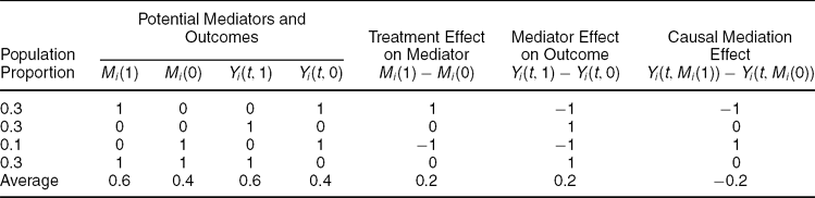
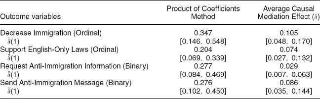
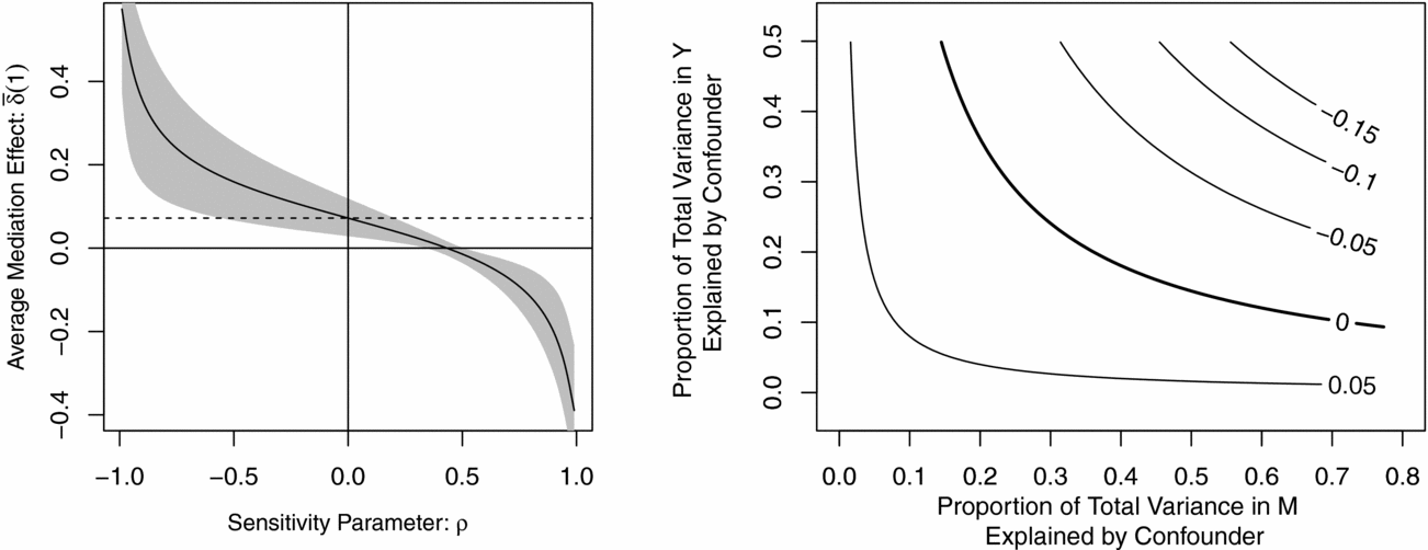
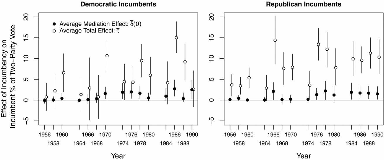
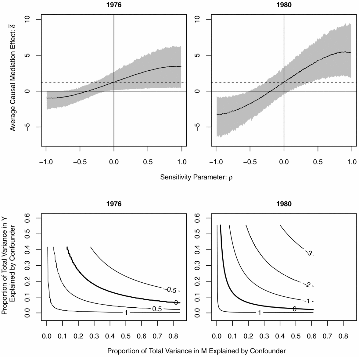
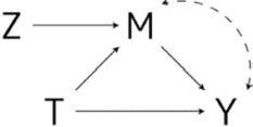
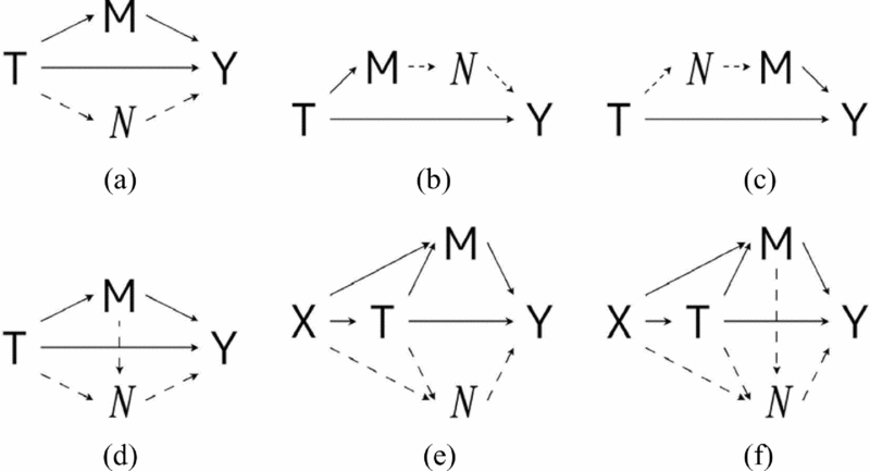
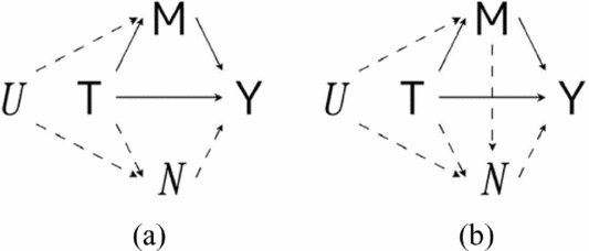
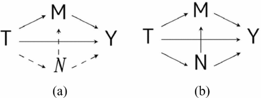



Comments
No Comments have been published for this article.