







1. Introduction
Vortex shedding phenomena in flows over axisymmetric bodies are a critical component to engineering design due to various implications on hydrodynamic and aerodynamic loading and stability. Similarities in vortex shedding events are well documented over a range of axisymmetric shapes including spheres, ellipsoids, cylinders and cones. A circular disc, the subject matter of the current work, may be considered the limiting case of the cone family, i.e. a cone with a half-angle of  $90^\circ$. Flows over spinning discs can be observed in many applications including, but not limited to, micro air vehicles, frisbees and drones. Understanding of the intrinsic flow characteristics is necessary to predict the aerodynamic loading in such applications.
Generally, a disc in axial flow acts as an obstruction by deflecting incoming flow radially outwards. As the angle of incidence is increased, the disc presents less of an obstruction to the incoming flow. With the addition of spin, the disc acts as a centrifuge that draws in the incident fluid and expels it radially outwards to satisfy continuity. In doing so, spin and angle of incidence act as precursors of angular and linear momentum that can significantly influence vortex shedding phenomena and wake structure. In this study, the effects of spin and angle of incidence on the flows upstream of a finite circular disc at a moderate Reynolds number are explored to quantify their influences.
Periodic motions in the wakes of circular discs are well documented and are attributed to vortex shedding originating from separated shear layer instabilities. Several experimental studies have employed flow visualization techniques that have illuminated the three dimensionality of the shedding vortices; they have been consistently described as linked chains of irregular vortex rings (Marshall & Stanton Reference Marshall and Stanton1931; Willmarth, Hawk & Harvey Reference Willmarth, Hawk and Harvey1964; Calvert Reference Calvert1967; Berger, Scholz & Schumm Reference Berger, Scholz and Schumm1990; Miau et al. Reference Miau, Leu, Liu and Chou1997). Vortex shedding in loop-like structures is not exclusive to flows over discs; it has also been observed in the wakes behind spheres and other axisymmetric thick and slender bodies (Willmarth et al. Reference Willmarth, Hawk and Harvey1964; Pao & Kao Reference Pao and Kao1977; Perry & Lim Reference Perry and Lim1978; Taneda Reference Taneda1978). It is commonly accepted that loop-like vortical structures characterize the wakes behind axisymmetric bluff bodies.
At low Reynolds numbers,  $\textit {Re} \lesssim 100$, flows over circular discs are steady. Within this regime, re-circulation bubbles form in the wake region and remain attached to the downstream surface of the disc (Fail, Lawford & Eyre Reference Fail, Lawford and Eyre1959). As the Reynolds number increases, a transition to a chaotic regime quickly develops. With the added complexities of this transition, variability of results within the literature are more apparent. Over a short range of the Reynolds number,
 $100 \lesssim \textit {Re}\lesssim 300$, up to seven bifurcation modes and regimes have been reported (Natarajan & Acrivos Reference Natarajan and Acrivos1993; Fabre, Auguste & Magnaudet Reference Fabre, Auguste and Magnaudet2008; Shenoy & Kleinstreuer Reference Shenoy and Kleinstreuer2008; Meliga, Chomaz & Sipp Reference Meliga, Chomaz and Sipp2009; Chrusy, Bouchet & Dušek Reference Chrusy, Bouchet and Dušek2010). Gao et al. (Reference Gao, Tao, Tian and Yang2018) concisely summarize five regimes and their critical Reynolds numbers,
 $\textit {Re}_c$, from a direct numerical simulation (DNS) study: steady state,
 $\textit {Re}_{c1} \approx 120.5$; periodic state,
 $128.5 < \textit {Re}_{c2}< 130$; periodic state with low frequency modulation,
 $140<\textit {Re}_{c3}<141.5$; quasi-periodic state,
 $185<\textit {Re}_{c4}<190$; and chaotic state,
 $210<\textit {Re}_{c5}<215$. This range of Reynolds numbers puts the majority of experimental works in the chaotic state regime.
Zhong & Lee (Reference Zhong and Lee2012) visualize the wakes of freely falling circular discs in quiescent water with fluorescent dye over a range of Reynolds numbers,  $40<\textit {Re}<200$. Within this range, a few comparisons to available computational results in the literature are made and two bifurcation regimes are identified. An experimental study on the chaotic dynamics of falling discs with specific emphasis on their trajectories has been conducted by Field et al. (Reference Field, Klaus, Moore and Nori1997). In their work, discs falling in a glycerine–water mixture are reported to undergo four distinct types of motion: steady falling, periodic oscillating, chaotic and tumbling. The modes of falling are likely coupled to varying modes of vortex shedding, but this is not investigated in depth. Flows over a fixed disc at zero incidence, measured from the disc normal, can be used to model flows over falling discs. However, a freely falling disc will inevitably experience a change in relative velocity in the presence of atmospheric disturbances or due to the upstream effects of vortex shedding.
The study of flows over discs at incidence was first studied by the smoke visualization, hot-wire anemometer and pressure probe experiments of Calvert (Reference Calvert1967). In this work, a range of angles of incidence between  $0^\circ$ and
 $50^\circ$ are considered at Reynolds numbers between 500 and 1000 for flow visualization experiments and
 $3.5\unicode{x2013}5.0 \times 10^4$ for velocity and pressure measurements. Irregularly shaped vortex rings interlinked with one another are visualized in the wake regions of a disc at incidence. The frequency and strength of the shedding vortices are reported to increase with the angle of incidence. Through careful selection of reference velocity and length scale, a constant wake Strouhal number equal to 0.21 is observed up to
 $40^\circ$ angle of incidence. The wake Strouhal number was computed with a reference velocity outside of the wake of the disc at the longitudinal position where the static pressure on the centreline was a minimum. The measured width of the wake was the chosen length scale. Similarly, both Abernathy (Reference Abernathy1962) and Knisely (Reference Knisely1990) observe a constant Strouhal number of
 $St\approx 0.15$ for thin rectangular cylinders (two-dimensional; 2-D) up to
 $75^\circ$ incidences. Gao et al. (Reference Gao, Tao, Tian and Yang2018) provide DNS results and Chrust et al. (Reference Chrust, Dauteuille, Bobinski, Rokicki, Goujon-Durand, Wesfreid, Bouchet and Dušek2015) provide further numerical and experimental results for flows behind inclined discs.
Further complications arise with the addition of rotation. Bodies of revolution exhibit three-dimensional (3-D) boundary layer transitions through various forms of instability. Initial efforts to understand the boundary layer transition over axisymmetric bodies began with spinning discs (Gregory, Stuart & Walker Reference Gregory, Stuart and Walker1955) and spinning spheres (Kohama & Kobayashi Reference Kohama and Kobayashi1983) in quiescent media. Moreover, Savaş (Reference Savaş1987) presents an experimental investigation of Bödewadt flow, rotating flow over a stationary disc, where instabilities are observed to take the form of circular waves at low Reynolds numbers, and a combination of circular and spiral waves at high Reynolds numbers. Beyond the boundary layer, spinning discs induce flow towards the surface and expels it radially outward due to centrifugal forces. Similarity formulations of incompressible viscous flows over stationary and spinning discs are taken up later in this paper (Hiemenz Reference Hiemenz1911; Kármán Reference Kármán1921; Cochran Reference Cochran1934; Hömann Reference Hömann1936; Hannah Reference Hannah1947). Gregory & Walker (Reference Gregory and Walker1960) conducted an experimental investigation of the centrifugal effect of a spinning disc in quiescent fluid. Axisymmetric stagnation point flows over spinning discs at incidence have been studied by reduction of the Navier–Stokes equations through similarity transformations (Niimi, Minamiyama & Hanai Reference Niimi, Minamiyama and Hanai1981; Sarkar & Sahoo Reference Sarkar and Sahoo2021). Raghav & Komerath (Reference Raghav and Komerath2013) provided planar velocity measurements of corotating vortical structures emanating from the leading edge of a spinning disc in upstream flow at  $8^\circ$ angle of incidence (
 $98^\circ$ using this paper's definition of the angle of incidence below).
More recently, Lee (Reference Lee2022) studied the instabilities in flow over a spinning disc at incidence by employing the immersed-boundary lattice Green's function (IBLGF) method. This work is motivated by the application to micro air vehicles, which exploit the spin-stabilization characteristics of spinning discs. The study focuses on low Reynolds numbers of  $O(10^2)$ with rotational speed ratios up to 3. Several observations are made, with emphases on the distinct wake regimes attributed to vortex shedding, and their relation to the effects of spin and the resulting aerodynamic forces acting on the disc. With increasing rotational speed ratio, monotonic increases in both lift and drag, where the lift-to-drag ratio remained constant, are observed. Spin is observed to suppress vortex shedding into the wake region by aiding in the dissipation of vorticity. An elliptic instability in the trailing tip vortices is observed for the spinning disc cases, not persistent in the non-spinning cases, where spin acts as additional forcing to the instability.
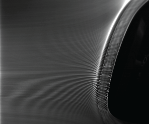
Several studies exist on the flows behind stationary circular discs at incidence with particular emphasis on vortex shedding phenomena in the wake region. However, studies over the upstream surface of discs are limited. Additionally, studies on the centrifugal effects of spinning discs in uniform flow at incidence are scarce. This study aims to present a source of reference flows over a spinning disc at incidence at a moderate Reynolds number, which may be considered the limiting case for the parametric study of flows over spinning cones at incidence as a function of the vertex angle. A smoke-wire flow visualization (FV) technique is used to generate a sheet of smoke streaklines and visualize the flows. A planar particle image velocimetry (PIV) technique is used to make velocity measurements over the surface of the disc. Hot-film anemometry is employed to determine shedding frequencies in the wake region.
Incompressible potential flow and viscous flow solutions over a spinning disc at zero incidence are reviewed in § 2. The smoke-wire, planar PIV and hot-film anemometry experimental set-ups and procedures are described in § 3. Results and observations from the smoke visualization experiment are presented in § 4, PIV results and analyses in § 5, and hot-film anemometry results and analyses in § 6. Streaklines from the smoke visualization experiments and streamlines computed from the PIV measurements are compared with incompressible potential flow streamlines to gauge the success of the experiments. Similarity solutions of viscous flows over spinning discs are also compared with velocity measurements. Lastly, closing remarks and conjectures are presented in § 7.
2. Theoretical background
2.1. Definitions and flow parameters
Figure 1 shows a schematic of a disc and its relevant coordinate systems and flow parameters. A wind tunnel-fixed Cartesian coordinate system  $(x,y,z)$ is centred on the upstream face of the disc. The
 $x$-axis is aligned with the free stream,
 $U_\infty$, and is positive in the downstream direction. The
 $y$-axis is positive to the right looking upstream; the
 $z$-axis is positive up. The disc spins at an angular speed of
 $\varOmega$, where the positive direction of rotation is defined clockwise looking upstream. Zero incidence corresponds to a free stream normal to the disc. As the angle of incidence,
 $\alpha$, is increased, the trailing edge of the disc moves in the downstream direction. The velocity fields over the disc are described in reference to a disc-fitted Cartesian coordinate system
 $\boldsymbol {u}(x_*,y_*,z_*)=(u_{x_*},u_{y_*},u_{z_*})$ shown in the figure. Hence, the disc-parallel (radial) and disc-normal (axial) components of the velocity vector are defined along the disc-fitted coordinate system
 $(x_*,y_*,z_*)$ as
 $( u_\parallel, u_\perp ) =(u_{x_*}, -u_{z_*})$. Finally, a disc bound spherical polar coordinate system
 $(r,\theta,\phi )$ is also defined and used in review of an axisymmetric potential flow solution in § 2.2 below. Note that
 $(r,\theta ={\rm \pi},\phi )$ corresponds to the
 $z_*$-axis.
Definitions of wind tunnel-fixed,  $(x,y,z)$, and disc-fitted,
 $(x_*, y_*, z_*)$, coordinate systems. The disc surface is in the
 ${z_*=0}$ plane. The hot-film probes are positioned at
 $(x/D, y/D,z/D) \approx (1.5,0,1.1)$ for the straight probe and at
 $(x/D, y/D,z/D) \approx (1.5,0,1.3)$ for the bent probe.

The Reynolds number based on the diameter of the disc,  $D=20.3$ cm, is defined as
 \begin{equation} \textit{Re} = \frac{U_\infty D}{\nu}, \end{equation}
where  $\nu$ is the kinematic viscosity (
 $\nu =0.15\,\text {cm}^2\,\text {s}^{-1}$ for air). The rotational speed ratio at the edge of the disc is defined as
 \begin{equation} S = \frac{\varOmega \, D / 2}{U_\infty}, \end{equation}
the ratio of the azimuthal velocity at the edge and the free stream velocity. When presenting the current vortex shedding results below, Strouhal number
 \begin{equation} St = \frac{f\, D }{U_\infty}, \end{equation}
based on the frequency  $f$ in Hz, disc diameter
 $D$ and the free stream velocity
 $U_\infty$, is used. As indicated earlier, there are variations in the literature on the selection of the length and velocity scales.
A series of smoke visualization and PIV experiments are conducted at  $U_\infty = 2\,{\rm m}\,{\rm s}^{-1}$ and a range of incidence angles
 $0\leq \alpha \leq 36^\circ$. The disc Reynolds number is
 $\textit {Re} = 2.7\times 10^4$. The angular speed of the disc is set to obtain speed ratios of
 $S=0, \pm 2,4,8 \text { and } \ 10$. Uncertainty of the smoke/laser sheet location with respect to the disc's axis of rotation persists, thus at
 $S=\pm 2$, the disc is spun in both clockwise and counter clockwise directions to confirm symmetry of the flows. This validation is taken up later in the paper when discussing PIV constructed velocity fields.
2.2. Incompressible potential flow over a disc
The axisymmetric incompressible potential flow solution over an infinite disc may be derived as a solution to Laplace's equation in spherical polar coordinates for the potential function  $\varphi (r,\theta )$ (Whitehead & Canetti Reference Whitehead and Canetti1950; Rosenhead Reference Rosenhead1963). The resulting expressions for the potential function, stream function and velocity vector are respectively
 $$\begin{gather} \varphi = {\tfrac{1}{2}} ar^2(3 \cos ^2 \theta -1 ), \end{gather}$$
 $$\begin{gather}\psi = ar^3 \sin ^2 \theta \cos \theta, \end{gather}$$
 $$\begin{gather}(u_r, u_\theta)=\left( a r (3\cos^2 \theta -1 ), \ -3ar \sin \theta \cos \theta \right). \end{gather}$$
For comparison with measurements later, the velocity vector may be written in components along the disc-fitted Cartesian coordinate system  $(x_*,y_*,z_*)$ as
 \begin{equation} {\boldsymbol u}(x_*,y_*,z_*)=(u_{x_*},u_{y_*},u_{z_*})=({-}ax_*, -ay_*, 2az_*), \end{equation}
which is the classical axisymmetric stagnation potential flow over a plane. The corresponding flow field has a uniform and constant strain rate tensor
 \begin{equation} e_{ij} = \begin{pmatrix} -a & 0 & 0 \\ 0 & -a & 0 \\ 0 & 0 & 2a \end{pmatrix} . \end{equation}
Thus, the role of the constant  $a$ now becomes clearer as the sole strain rate parameter. The upstream potential flow is not uniform, in contrast to the uniform upstream flow in the case of the wind tunnel experiments described here.
2.3. Incompressible viscous flow over a disc
A similarity solution of the steady viscous flow induced by a spinning infinite disc in quiescent fluid is presented by Kármán (Reference Kármán1921) and Cochran (Reference Cochran1934). Axisymmetric stagnation point flow over a non-spinning disc is introduced by Hömann (Reference Hömann1936), following its two-dimensional counterpart by Hiemenz (Reference Hiemenz1911). A general viscous formulation of steady irrotational axisymmetric flow against a spinning infinite disc is presented by Hannah (Reference Hannah1947), where the above solutions are two special cases.
Hannah (Reference Hannah1947) develops the general solutions using a cylindrical polar coordinate system,  $(r,\theta,z)$. The disc is defined at
 $z = 0$ and rotates with constant angular speed,
 $\varOmega$, about its central axis (
 $r=0$) in the presence of approaching axial flow
 $u_{z_*}=-u_\perp =2az_*$. A dimensionless rotation parameter is defined as
 $\mu = \varOmega / a$, where
 $a$ is the strain parameter of the approaching flow. Hence,
 $\mu = 0$ corresponds to the Hömann flow and
 $\mu = \infty$ to the Kármán flow. Hannah (Reference Hannah1947) presents numerical solutions for values
 $\mu = 0, 1/2, 1, 2\ \text {and}\ \infty$. The tangential, axial and radial velocity profile similarity functions;
 $G(\zeta )$,
 $N(\zeta )$ and
 $N^\prime (\zeta )$, respectively; against the disc-normal spatial coordinate
 \begin{equation} \zeta \equiv (1+\mu^2)^{{1}/{4}}\left[\frac{a}{\nu}\right]^{{1}/{2}} z_* \end{equation}
are produced in Hannah's notation in figure 2(a–c) for reference, which include  $\mu$ corresponding to zero incidence,
 $S=0,2,4,8\text { and } 10$ cases, and
 $\mu = \infty$ corresponding to the limiting case of Kármán flow.
(a) Tangential,  $G(\zeta )$, (b) axial,
 $N(\zeta$), and (c) radial velocity,
 $N'(\zeta )$, profiles over a spinning disc in axial flow for selected values of the rotation parameter
 $\mu$, using the notation of Hannah (Reference Hannah1947) for the profile functions
 $G(\zeta )$,
 $N(\zeta )$ and
 $N'(\zeta )$. The profiles for
 $\mu =0, 5.3, 10.6, 21.3\text { and } 26.6$ correspond to
 $S=0, 2, 4, 8\text { and } 10$ spinning disc cases at zero incidence discussed within the present work. Panel (d) is a normalized comparison of profiles for axisymmetric stagnation point flow (Hömann Reference Hömann1936) and rotating disc cases (Hannah Reference Hannah1947). The boundary layer thickness in panel (d) for
 $\mu =0$ is
 $\zeta _{0.99}\approx 2.0$ and for
 $\mu =5.3$,
 $\zeta _{1.01} \approx 4.0$.

The disc produces two distinct effects on the upstream velocity field depending on  $\mu$. In the first extreme (
 $\mu = 0$), a non-spinning disc in axial flow deflects the incoming flow by acting as an obstruction. Here, viscous forces near the surface oppose the direction of flow due to the no slip condition at the surface. In the second extreme (
 $\mu = \infty$), a spinning disc in quiescent fluid facilitates upstream flow by expelling flow in the outward radial direction and suctioning upstream fluid to satisfy continuity. These effects are in constant opposition to one another over the full range of
 $\mu$ and are displayed through the resulting velocity profiles. Note that in the similarity solution, the axial component of velocity continually increases away from the surface of the disc in all cases where
 $\mu \neq \infty$, unlike the uniform upstream flow in the wind tunnel experiments presented here. The centrifugal effects in the experiments are observed up to a finite distance from the surface of the disc.
Normalized boundary layer profile functions of flows normal to a fixed infinite disc ( $\mu =0$, axisymmetric stagnation point flow (Hömann Reference Hömann1936) corresponding to
 $S=0$) and to a rotating infinite disc (
 $\mu =0, 5.3, 10.6, 20.3\text { and } 26.6$ corresponding to
 $S=0, 2, 4, 8\text { and } 10$, respectively) are plotted in figure 2(d) in their respective similarity coordinates given in (2.9). For later reference, the boundary layer thickness in the similarity coordinate in the figure for
 $\mu =0$ is
 $\zeta _{0.99}\approx 2.0$ and for
 $\mu =5.3$ is
 $\zeta _{1.01} \approx 4.0$.
3. Experimental set-ups and procedures
Smoke visualization, planar PIV and hot-film anemometry experiments are conducted in an open-return, low-speed wind tunnel with an  $82W\times 82H\times 365L \,{\rm cm}^3$ rectangular test section and a
 $14:1$ contraction ratio. The tunnel allows for speeds up to
 $20\,{\rm m}\,{\rm s}^{-1}$ with low turbulence levels and is capable of maintaining speeds at
 $2\,{\rm m}\,{\rm s}^{-1}$ and lower, which is essential for smoke visualization experiments. The experiments discussed here are all carried out at a tunnel speed of
 $200\pm 5\,{\rm cm}\,{\rm s}^{-1}$.
3.1. Disc model
The disc model, sketched in figure 1, is 1.5 cm thick, 20.3 cm in diameter and machined from acrylonitrile butadiene styrene (ABS). Thus, the thickness ratio is  $t=1.5/20.3=0.074$. Its rear edge is chamfered at
 $45^\circ$. A connecting feature is machined on the downstream face of the disc to allow for a press fit attachment to an AC-servomotor (Leadshine ACM604V60-01) that spins it under computer control. The disc is sanded to a smooth finish and coated with satin black paint for enhanced smoke streak visualization. It is then coated with a translucent fluorescent paint, which is a mixture of rhodamine dye and water solution with polyurethane. Fluorescent paint is used to mitigate overexposure effects near the surface of the disc from reflected laser light during PIV runs (more details are presented in § 3.3). The disc-motor assembly is attached to a 1.9 cm diameter sting, which is held by a rack and indexing mechanism. The indexing mechanism allows for a range of angles of incidence,
 $-6^\circ \leq \alpha \leq 36^\circ$ at
 $3^\circ$ increments while keeping the centre of the disc centred in the tunnel test section. The experiments reported here are done at
 $\alpha =0,6,12,18,21,24,30 \text { and } 36^\circ$. The disc model and its attachments present
 $\sim 7\,\%$ asymmetric blockage to the tunnel flow.
3.2. Smoke visualization
A smoke-wire set-up is used to visualize the flow by generating a sheet of thin and uniformly spaced smoke streaklines in the test section. The smoke-wire consists of a pair of 0.25 mm diameter 316-stainless-steel wires, twisted to approximately 4 mm pitch. The pair is 120 cm long and stretches vertically through the test section under the tension of a mass attached to its lower end outside the test section. It is positioned 27 cm upstream of the disc and aligned with the disc's central axis with a  $y$-axis linear translation stage. A 50/50 by volume glycerin–water mixture is dripped onto the wire pair and vaporized by supplying
 $\sim$50 V via an AC rheostat (3.4 amperes). A series of streaklines form approximately 2 mm apart in two interleaving sets, differing slightly in intensity and in slightly separated planes. The smoke streaklines last approximately 3 seconds, allowing ample time for high speed image acquisition. No vortex shedding signatures are detected over the twisted wire pair throughout this investigation due to low wire Reynolds number
 $({\sim }35)$. More details of the smoke-wire technique may be found from Kuraan & Savaş (Reference Kuraan and Savaş2019).
Two cameras are used in the smoke visualization experiments to capture images from two different viewing angles. An IDT MotionPro Y-Series camera, capable of capturing  $1280 \times 1024$ pixel images at speeds of up to 6000 frames per second (fps), is used to capture smoke streakline images in the
 $xz$-plane. With this camera, a 50 mm Canon lens is used to capture full view images of the disc at 600 fps with a field of view of
 $34 \times 27$ cm along the
 $x$ and
 $z$ directions, respectively. A circular polarizing filter is used to reduce glare from reflecting surfaces. A GoPro Hero3+ camera is used to capture smoke visualization images at oblique angles upstream of the disc with
 $1920 \times 1080$ pixel resolution at 60 fps. The GoPro camera is mounted to the left-hand side of the test section (
 $-y$ direction) and slightly above the central axis of the test section (
 $z\approx 0$), allowing for a downstream viewing angle of the disc at approximately a
 $30^\circ$ angle in the
 $xy$-plane. Barrelling distortions introduced by the GoPro camera's wide-angle lens are removed using various commercial software packages.
Two light sources are used: an LED flood light (1300 lumens), positioned normal to the smoke streakline plane ( $xz$-plane), and two Quasar Science flicker-free LED lights mounted to the test section ceiling and positioned directly above the disc. To further enhance imaging, the inner surfaces of the test section are lined with black felt.
The recorded images are processed for optimum visualization of the smoke streaklines using open source image processing and analysis packages, ImageJ Fiji, (Schindelin et al. Reference Schindelin2012; Schneider, Rasband & Eliceiri Reference Schneider, Rasband and Eliceiri2012; Rueden et al. Reference Rueden, Schindelin, Hiner, DeZonia, Walter, Arena and Eliceiri2017). In this processing, image backgrounds are subtracted, and brightness and contrast are adjusted for clarity.
3.3. Particle image velocimetry
A planar PIV technique is used for velocity measurements over the surface of the disc. Table 1 lists the PIV parameters. The same IDT MotionPro Y-Series digital camera that was used for the smoke visualization experiments is used here too. An 85 mm Nikon lens is attached to the camera with a 10 mm spacer. The PIV region of interest overlaps that of the FV. The camera lens is positioned approximately 50 cm from the laser sheet and captures a field of view of  $7.2\,{\rm cm} \times 9\,{\rm cm}$, in the
 $x$ and
 $z$ directions, respectively. The flow field is illuminated with two overlapping laser sheets generated from a dual-head, pulsed Nd:YAG laser.
PIV set-up summary.

Fine tuning of the PIV test set-up is necessary to capture sufficient scattered light from the micron sized seeding droplets, while reducing the effects of reflected light from surfaces. To reduce loss of light from internal reflections, a  $5\times 2$ cm slit is cut out from the test section's acrylic sheet ceiling to eliminate reflections. Similarly, a
 $31\times 25$ cm section is removed from the acrylic test section side window and then covered with a 3 mm thick high efficiency anti-reflective window. Overexposure effects of reflecting laser light near the surface of the disc are reduced using a fluorescent paint and filtering technique (Paterna et al. Reference Paterna, Moonen, Dorer and Carmeliet2013; Bisel et al. Reference Bisel, Dahlberg, Martin, Owen, Keanini, Tkacik, Narayan and Goudarzi2017). The disc is coated with translucent fluorescent paint that reflects incoming laser light at longer wavelengths. The reflected light is filtered out with a bandpass filter (532 nm CWL, 25 mm diameter), which is fitted into the C-mount of the camera lens.
The laser head is mounted on two linear stages at the tunnel roof that allow for translation in  $x$ and
 $y$ directions. The camera is attached to a linear stage that allows for change in elevation (
 ${\pm }z$-direction). All linear stages can be driven by DC micro-stepper motors (Compumotor M83-135) under computer control. The laser beams are focused with a spherical lens and passed through a cylindrical lens (
 $f = 500$ mm) to generate laser sheets that are approximately 2 mm thick. The overlapping sheets are redirected with a 25 mm diameter circular mirror into the test section.
The firing rate of the lasers and image capture rate of the camera are synchronized using a counter card (Computer Boards CIO CTR-10). Image pairs,  $400\,\mathrm {\mu }{\rm s}$ apart, are captured at 30 Hz. This sampling rate is sufficient for obtaining the mean flow fields. However, it is too low to capture the unsteady behaviour of the vortices discussed below. A Laskin nozzle atomizer (PIVTEC GmbH Aerosol Generator PivPart30 series) is used to atomize di-ethyl-hexyl-sebacic-acid-ester (DEHS, density of 0.92 g cm
 $^{-3}$) into micron-sized droplets that are used to seed the wind tunnel. The atomizer is positioned near the wind tunnel fan during normal operations. As the wind tunnel is open-return type, the whole laboratory is seeded with the DEHS droplets.
The image preprocessing method, proposed and validated by Mendez et al. (Reference Mendez, Raiola, Masullo, Discetti, Ianiro, Theunissen and Buchlin2017), is applied to remove background noise and further reduce the effects of laser light reflections near surfaces. The method is based on the proper orthogonal decomposition (POD) of image sequences and makes use of the different spatial and temporal consistency of background and particles. Unlike the traditional methods, POD-based filtering is insensitive to time varying, sharp reflections and for cases where background noise is brighter than the particle images. Due to inevitable differences between laser sheets generated from the two laser heads, each image pair is separated before filtering. The backgrounds of each image set are identified from the POD decomposition and used to reconstruct filtered image pairs. Making use of the background images, a binary image mask is generated using commercial software packages to determine the air–disc interface.
PIV data analysis is carried out using an inhouse adaptive Lagrangian parcel tracking software package (Sholl & Savaş Reference Sholl and Savaş1997; Ortega, Bristol & Savaş Reference Ortega, Bristol and Savaş2003; Bardet, Peterson & Savaş Reference Bardet, Peterson and Savaş2010, Reference Bardet, Peterson and Savaş2018; Ibarra, Shaffer & Savaş Reference Ibarra, Shaffer and Savaş2020). In the current application, autonomous adaptability of the interrogation area (IA) is implemented. During this process, the IA size is reset based on the initial interrogation size of  $32 \times 32$ pixels. The initial IA size is chosen to ensure that aggregate particle displacement is smaller than 1/4 of the IA dimension. Based on the result from the initial step, the interrogation window can be shrunk down to as small as
 $8\times 8$ pixels at very low velocities, or increased to
 $64\times 64$ pixels at very high velocity regions. In the final adaptive pass, the spatial resolution is no longer uniform, which is the case in low velocity regions as the final window size is kept at a minimum of 4-times the displacement. In particular, smaller windows in the boundary layers and at the stagnation points ensure independent velocity vector measurements for there is no overlap at
 $16\times 16$ pixels step sizes. The uncertainty in velocity measurements are estimated to be less than
 $2\,{\rm cm}\,{\rm s}^{-1}$. Postprocessing is done using various commercial software packages. Most PIV results presented in this paper are time averages.
3.4. Hot-film anemometry
Hot-film measurements are taken downstream of the disc's trailing edge to determine shedding frequencies for comparison with the upstream observations from the PIV and smoke visualization experiments. Two TSI hot-film probes, Model 1210-20W (general purpose straight probe) and Model 1212-20W (standard single sensor probe with bent sensor needles), with TSI-1054A/1056 constant temperature anemometry (CTA) bridge circuitry, are used to make measurements (TSI 2013). Both probes are mounted to the wind tunnel ceiling and their sensors are located at  $(x/D, y/D, z/D) \approx (1.5, 0, 1.1)$ for the straight probe and at
 $(x/D, y/D,z/D) \approx (1.5, 0, 1.3)$ for the bent probe, where
 $D=20.3$ cm. The positions of the probes were chosen following flow visualization runs to locate the trajectories of the vortices shed off the disc. The positions are chosen such that the sensors are at the edge of the vortical wake, registering sufficiently large fluctuation amplitudes of signals without destroying the vortices themselves. The probes are calibrated against a Pitot-static tube in the wind tunnel. Measurements are taken simultaneously from the probes at 512 Hz for a duration of 12 s for each run. The raw signals are recorded along with corresponding filtered signals that are bandpass filtered over the range 0.1–20 Hz. They have ample frequency response, which are used to generate power spectra for all
 $(\alpha, S)$ cases.
4. Flow visualization
Figure 3 shows smoke visualization images captured normal to the  $xz$-plane over a range of angle of incidence,
 $0\leq \alpha \leq 36^\circ$. Note, the pitch of the smoke streaks in figure 3(c) is wider than the rest of the sequence for it was taken after rearrangement of the set-up. Figure 4 shows images captured with a downstream viewing angle over the same range of
 $\alpha$, but in
 $12^\circ$ increments. Each figure displays a set of images at the same
 $\alpha$, showing the fixed and two spinning cases;
 $S=0 \text { and } \pm 2$.
Streakline patterns over the disc:  $\textit {Re} = 2.7 \times 10^4$,
 $S=0 \text { and }\pm 2$, and (a–e)
 $\alpha = 0, 12, 21, 24 \text { and } 36^\circ$. The disc edge is outlined with bold white lines in panel (a i,b i,c i,d i,e i) to aid visualization and illustrate the change in
 $\alpha$. Coherent vortical structures form at the pressure side, upstream surface, of the disc and cyclically shed into the wake region. The images shown here correspond to frames where vortical structures are aligned with the disc's central axis, prior to being shed into the wake region. The first instance (
 $\alpha =0$ and
 $S=0$) is annotated to direct the reader's attention to the referenced vortical structures. The reader is encouraged to watch Movie 1 and Movie 3 to develop familiarity for the viewing angle in which the flow fields are captured here.

Streakline patterns over the disc at an oblique downstream viewing angle.  $\textit {Re} = 2.7 \times 10^4$,
 $S=0 \text { and } \pm 2$, and (a–d)
 $\alpha = 0, 12, 24 \text { and } 36^\circ$. The image in panel (ai) (
 $\alpha =0$ and
 $S=0$) is annotated to aid visualization. Coherent vortical structures form at the pressure side, upstream surface, of the disc and cyclically shed into the wake region. The images shown here correspond to frames where vortical structures are aligned with the disc's central axis, prior to being shed into the wake region. The reader is encouraged to watch Movie 2 and Movie 4 to develop familiarity for the viewing angle in which the flow fields are captured here.

All flows over the disc are unsteady. The flows exhibit vortical structures of varying complexity at all incidence angles. These structures start out as cylindrical vortices, evolve into sinuous modes, exhibit solitary patterns, show finer scale signatures of cross-flow instabilities and eventually are shed into the wake. Two vortex shedding modes are observed; the first mode will be described in reference to figure 3(a) and the second in reference to figure 3(e). The finer scales are thought to be signatures of cross-stream instabilities riding the dominant modes of vortex shedding; they will not be discussed in detail for they are beyond the scope of this work.
4.1. Non-spinning disc cases,  $S=0$

At  $\alpha =0$ incidence in figure 3, an unsteady flow is observed near the surface of the disc that is marked by a cyclic, into and out of the symmetry plane motion (
 $\pm$
 $y$-directions). As the sheet of uniform streaklines approach the surface of the disc, it coils onto itself and marks the coherent vortical structures or rolls. These structures maintain their integrity as they are shed into the wake region of the disc at approximately 2 Hz, corresponding to a Strouhal number based on the diameter of the disc of approximately 0.2. Over approximately three quarters of the shedding period, the vortical structures grow in size and align themselves parallel to the disc surface. Over the remaining quarter of the shedding period, they are rapidly swept by the mean flow into the wake region in the
 $\pm y$-directions. The shedding directions are difficult to detect in the normal viewing angle in figure 3 as vortical structures shed away from the camera's focal plane; however, they are tractable from the downstream viewing angle in figure 4.
Figure 3(b,d) shows for  $S = 0$, a clear image of the vortex as marked by streaklines, both intact and bursting at the core. Sketches depicting the shape and orientation of the vortical structures over a typical shedding period through the first mode of vortex shedding are shown in figure 5. During the shedding process, the vortical structures deform from straight lines to bimodal ones, with peaks near the edge of the disc. The radial velocities,
 $u_\parallel$, of stagnation point flows increase in the radial direction away from the stagnation point. As the bimodal vortex filaments approach the wake region, they are reshaped into an arc, with their ends extending into the wake region.
Sketch illustrating the first mode of vortex shedding near the upstream surface of a disc at low angles of incidence. (i) Vortical structures originate near the disc's axis of symmetry and align themselves parallel to the surface of the disc. Once they have grown past a certain size, they shed radially outwards in unpredictable  $\pm y$-directions. (ii) During the shedding period, they deform from their originally linear alignment into a bimodal form. (iii) As they approach the outer edge, they reach a terminal arc form and shed into the wake region. Note that the illustrations of vortical formations are truncated. In the smoke visualization experiments, they are observed to extend into the wake of the disc.

The direction of vortex shedding is unpredictable. The randomness in shedding orientation and direction is requisite to satisfying the axisymmetric global property of the time-averaged flows in the wake of a fixed disc at zero incidence (Miau et al. Reference Miau, Leu, Liu and Chou1997). The asymmetric blockage of the articulating attachment mechanism, however small, may induce asymmetry in the flow conditions which may affect vortex formation, such as preferred shedding orientation. Figure 6 depicts sequential images of the life cycle of a vortex shedding event over a disc at zero incidence in both the normal and oblique-downstream viewing angles, where snapshots in figures 6(a) and 6(b) are equally spaced frames extracted from supplementary Movie 1 and Movie 2, respectively. The playback speed is reduced by a factor of 20 in Movie 1 and a factor of 10 for Movie 2. The vortex shedding events observed here are thought to be precursors to the well studied vortices in the wake of circular discs (Marshall & Stanton Reference Marshall and Stanton1931; Calvert Reference Calvert1967; Berger et al. Reference Berger, Scholz and Schumm1990; Miau et al. Reference Miau, Leu, Liu and Chou1997; Shenoy & Kleinstreuer Reference Shenoy and Kleinstreuer2008; Zhong & Lee Reference Zhong and Lee2012).
Image sequences through one cycle of the first vortex shedding mode over a stationary disc at zero incidence captured at two viewing angles. Snapshots displayed in panels (a) and (b) are pulled from supplementary Movie 1 and Movie 2, respectively, available at https://doi.org/10.1017/jfm.2024.916. The reader is encouraged to watch the movies to develop familiarity for the viewing angles captured here. (a) Normal viewing angle captured at 600 fps. The bold white lines outline the disc surface. (b) Downstream viewing angle captured at 60 fps. The white dashed lines highlight the cores of the vortical structures as they deform and shed into wake region, as sketched in figure 5.

At zero incidence,  $\alpha = 0$, the stagnation point is located at the centre of the disc. As the angle of incidence is increased, it monotonically shifts towards the leading edge of the disc (figure 3b–e). A similar vortex formation and shedding phenomena observed for the zero incidence case are also seen at angles of incidence up to
 $21^\circ$ with a marked distinction: the vortical structures form in increasingly larger sizes, forming further away from the surface of the disc. This may result in the stronger fluctuations in the wake region as observed by Calvert (Reference Calvert1967). In the cases where the interiors of the vortical structures are visible, they appear to exhibit a sausaging mode of instability as their cross-sectional diameters vary spatially and temporally. As the vortical structures form, their sizes reach a maximum near the stagnation points and decrease radially outwards before being shed into the wake region. The interactions between the mean flow and the local vortical structures may explain this behaviour: as the angle of incidence increases,
 $u_\parallel$ increases. An increase in
 $u_\parallel$ acts by accelerating the ends of the vortical structures radially outwards, stretching and shrinking them in the process.
Transition to the second mode of vortex shedding is clearly observed between  $\alpha = 18^\circ$ and
 $24^\circ$ (figure 3d). To further understand this transition, smoke visualizations at
 $\alpha = 21^\circ$ are recorded and added to the original test matrix (figure 3c), where streaklines are less densely spaced due to reduced pitch in the twisted smoke–wire pair. A sketch detailing this phenomena is shown in figure 7. In the highest case,
 $\alpha = 36^\circ$ (figure 3e), the second mode of shedding is most discernible. At this incidence angle, vortical structures aligned parallel to the disc surface still form, but with noticeably diminished cross-sectional sizes. Vortex shedding into and out of the plane are present, but are less pronounced. The second mode presents itself primarily in the form of a soliton on the vortical structures. The soliton emerges near the leading edge of the disc and its crest-like signature propagates towards the trailing edge.
A sketch of the second mode of vortex shedding near the surface of a disc at high angles of incidence. The illustration portrays a side view of a disc in the  $xz$-plane at
 $\alpha = 36^\circ$. A soliton originates on the vortical structures near the leading edge of the disc and sheds towards the trailing edge and into the wake region. The illustration depicts truncated vortical structures; however, they are observed to extend into the wake of the disc in the smoke visualization experiments.

The cross-sectional sizes of the large vortical structures, as estimated from the flow visualization data, range from  $0.15D$ for the cases of zero incidence to approximately
 $0.08D$ for the cases at
 $\alpha =36^\circ$ incidence angle. The sizes of the vortices are an order of magnitude larger than the boundary layer predicted by theory for steady flows (figure 2c,d).
Figure 8 depicts sequential images of the life cycle of a vortex shedding event over the disc at  $\alpha = 36^\circ$ in both the normal and downstream viewing angles, where the secondary mode of vortex shedding is dominant. Snapshots from figures 8(a) and 8(b) are sampled from supplementary Movie 3 and Movie 4, where their playback speeds are reduced by factors of 20 and 10, respectively. The shedding frequency of the secondary mode at
 $\alpha = 36^\circ$ nearly doubles in comparison to that of the first at zero incidence; estimated at 3.75 Hz from the smoke visualization. Signatures of vortex shedding are even noticeable into the wake regions behind the disc. This mode of vortex shedding may be a result of the vortex system induced by the reversed flow behind the wake of a disc at incidence, as described by Calvert (Reference Calvert1967). Differences in shedding frequencies at high angles of incidence might be attributed to an increased asymmetric obstruction to the flow from the attached servomotor and flow apparatus components.
Image sequences through one cycle of the second vortex shedding mode over a stationary disc at  $\alpha = 36^\circ$ captured at two viewing angles. Snapshots displayed in panels (a) and (b) are pulled from supplementary Movie 3 and Movie 4, respectively. The reader is encouraged to watch the movies to develop familiarity for the viewing angles captured here. (a) Normal viewing angle captured at 600 fps. The bold white lines outline the disc surface. The red triangles are used to mark the crest of the soliton as it traverses towards the wake region. (b) Downstream viewing angle captured at 60 fps.

4.2. Spinning disc cases, $S=\pm 2$.

With the addition of spin, the flows over discs at incidence vary slightly. Generally, the flows over spinning discs at incidence mimic those over a stationary disc. Periodic flows are still present at similar shedding frequencies; however, the introduced centrifugal forces affect the formation and decay of the vortical structures. The vortical formations replicate the orientations of structures over the stationary disc cases, but the switching of shedding direction becomes more frequent.
The centrifugal forces of spinning discs lead to cross-stream instabilities on the outer edges of the large vortical structures at angles of incidence up to  $21^\circ$. They form irregularly and appear to trigger further unsteady events. They are reminiscent of the classical Kelvin–Helmholtz shear layer instability (von Helmholtz Reference von Helmholtz1868; Thomson Reference Thomson1871). Figure 9 shows magnified images of the cross-stream instabilities riding the dominant shedding vortices. Figure 9(a) is a cropped region below the stagnation point from the flow visualization image at
 $\alpha =6^\circ$ (not shown here) and figure 9(b) is a cropped region above the stagnation point from column 3 of figure 3(b). The apparent asymmetry between
 $\pm S$ snapshots is a result of the unsteady shedding of vortices.
Details of centrifugal signatures riding the dominant shedding vortex structures. (a)  $\alpha = 6^\circ$,
 $S = -2$, below the stagnation point. (b)
 $\alpha = 12^\circ$,
 $S=-2$, above the stagnation point (column 3 of figure 3b).

Boundary layer velocity profiles over spinning discs are prone to various modes of instability that take the form of circular or spiral waves. Two modes of spiral waves over spinning discs have been studied in detail and are designated as Type I (Class B) and Type II (Class A) (Gregory & Walker Reference Gregory and Walker1960; Savaş Reference Savaş1987). The observed cross-stream instabilities may be signatures of these boundary layer instability modes. The centrifugal effects may weaken the vortical structures being shed into the wake region.
At higher angles of incidence, rotation seems to reduce the cross-sectional size of the vortical formations. An infinite rotating disc in forced flow incurs additional velocities towards the disc, negative  $z_*\text {-direction}$, which is then expelled in the radial direction to satisfy continuity (Hannah Reference Hannah1947). Near the stagnation point, zero incidence flow over a spinning disc is a good approximation to flow over an infinite disc at zero incidence. Thus, reduction in cross-sectional sizes for spinning discs may be attributed to increased radial velocities,
 $u_\parallel$. Hence, by the same mechanism explained for stationary discs at high angles of incidence, the vortical structures are further stretched and shrunk as they extend into the wake regions. Contrarily, with the addition of spin, the amplitude of the soliton marking the second mode of vortex shedding grows.
5. Velocity measurements
Figure 10 shows instantaneous velocity plots (streamlines over speed fields) at the  $y=0$,
 $xz$-plane during one vortex shedding cycle at 0.1 s intervals for
 $\alpha =0$, for the
 $S=0$ and
 $S=-2$ cases. The time window is chosen to span the course of a typical shedding cycle of
 ${\sim }0.5$ s, following the observations of the smoke visualization images captured over the non-spinning case at zero incidence. Hence, from left to right, the contours correspond to times
 $t = t_0 + [0.1, 0.2, 0.3, 0.4, 0.5]$ s, where
 $t_0$ corresponds to an arbitrary time during PIV image acquisition. The
 $t_0$ case is omitted as it coincides with the
 $t_0 + 0.5$ s case. At
 $S=0$, the flow pattern in figure 10 is nearly stationary, consistent with the streakline pattern in figures 3 and 6. In contrast, the flow pattern for
 $S = -2$ shows local extrema consisting of cross-stream instabilities clearly visible in the last frame of figure 3. Similar behaviour is also observable in the streakline patterns shown in figure 4.
Consecutive instantaneous velocity (streamlines over speed contours) plots at 0.1 s increments during one vortex shedding cycle: (a–e)  $S=0$ and ( f–j)
 $S=-2$ at
 $\alpha =0$.

Figure 11 provides a set of plots used to evaluate the sensitivity of the direction of  $\varOmega$ on the resulting flow field for the zero incidence,
 $S=0\text { and }\pm 2$ cases. The measurements are averages over 100 velocity vector planes from which velocity contours and profiles are extracted. It is noted here that the number of shed vortex cycles captured within 100 PIV samples at 30 Hz is not sufficient for a well-converged mean profile. Spectral analysis effects from of the inhouse PIV code induce measurement errors near the outer edges of the captured flow regions; hence, those areas are ignored by trimming the boundaries by approximately 0.5 cm. As noted earlier, the PIV sampling rate is too low to record, fully, the unsteady vortex dynamics inherent in the flows.
Velocity measurements over the disc at  $\alpha = 0$ incidence for
 $S=0\text { and }\pm 2$. (a–c) Streamlines over speed contours, (d,e) profiles at
 $z_*/D=[0.05, 0.20]$ with
 $0.05$ increments and ( f,g) profiles at
 $x_*/D=[-0.15, 0.15]$ with
 $0.05$ increments.

The velocity components in the disc coordinate system,  $(u_\parallel (x_*,z_*),u_\perp (x_*,z_*))$, are extracted from the velocity components in the wind tunnel (camera) coordinate system
 $(x,z)$ using bilinear interpolation. Shown in figure 11(a–c), in the wind tunnel coordinate system
 $(x,z)$, are the normalized velocity magnitude contour plots,
 $|{\boldsymbol u}|/U_\infty$ with overlaid streamlines, which provide direct visual comparison with their respective flow visualization images. Profiles of normalized velocity components
 $u_\perp (x_*/D)/U_\infty$ and
 $u_\parallel (x_*/D)/U_\infty$ at selected
 $z_*/D$ lines with
 $\sim 0.05$ increments are shown in the second row. Profiles of normalized velocity components
 $u_\perp (z_*/D)/U_\infty$ and
 $u_\parallel (z_*/D)/U_\infty$ at selected to
 $x_*/D$ lines with
 $\sim 0.05$ increments are shown in the third row. In each of the normalized
 $u_\perp (x_*/D)$ and
 $u_\parallel (z_*/D)$ velocity profile plots,
 $\varOmega =0$ cases are plotted with black circles,
 $+\varOmega$ with red triangles and
 $-\varOmega$ with blue squares. This allows for following the evolution of the velocity profiles and the effects of the direction of rotation along the radius of the disc and at varying distances upstream of the disc. The
 $u_\parallel (x_*/D)$ and
 $u_\perp (z_*/D)$ velocity profile plots for
 $S = 0\text { and }\pm 2$ are presented as scatter plots; a straight line is fitted to each scatter plot and its slope is measured, where
 $\kappa _x$ corresponds to the slope of
 $u_\parallel (x_*/D)$ and
 $\kappa _z$ to the slope of
 $u_\perp (z_*/D)$. The fitted non-dimensional slopes
 $\kappa _x$ and
 $\kappa _z$ are used to determine the strain rate parameters in the
 $x_*$ and
 $z_*$ directions, respectively.
At zero incidence, effects of spin are readily noticeable in the  $S=\pm 2$ cases in figure 11. Spin induces larger axial velocities,
 $u_\perp$, towards the disc when compared with the non-spinning case. This characterization is further demonstrated in each of the velocity profile plots, where the velocity profiles for
 $S=0$ exhibit consistently thinner boundary layers than their spinning counterparts. Additional axial velocities are clearly present from the spinning disc and can be tracked from the axial velocity profiles,
 $u_\perp$. Centrifugal effects are also detectable from the disc-parallel velocity profiles,
 $u_\parallel$, where the non-spinning velocity profiles are consistently thinner than the spinning cases. The centrifugal effects act by increasing the magnitude of velocity near the surface where the incoming flow is expelled through the boundary layer.
At zero incidence, good agreement between the opposing rotation directions,  $S=\pm 2$, is demonstrated by their overlapping velocity profiles. No dependency between the direction of rotation and velocity profile shape is detected, as expected. Given this validation, the direction of rotation is not further assessed for angles of incidence greater than zero. Instead, attention is focused on the effects of the change in magnitude of
 $\varOmega$, and hence
 $S$, on the resulting flow fields.
Figures 12–15 show PIV measurements corresponding to the flows presented in figure 3(a,b,d,e). Presentation across the figures is similar to figure 11; instead of plotting cases corresponding to  $S=0\text { and }\pm 2$, cases corresponding to
 $S=0, 2\text { and } 10$ are presented. Fifty additional velocity vector planes (150 total) are used in the time average results for these figures from which, again, velocity contours and profiles are extracted. Each figure shows various results at an angle of incidence
 $\alpha$. Shown in the first (top) row, in the wind tunnel coordinate system
 $(x,z)$, are the normalized velocity magnitude contour plots,
 $|{\boldsymbol u}|/U_\infty$, with overlaid streamlines for
 $S = 0,2\text { and } 10$, which provide direct visual comparison with their respective flow visualization images for
 $S = 0\text { and } 2$ in figure 3. In each of the normalized
 $u_\perp (x_*/D)$ and
 $u_\parallel (z_*/D)$ velocity profile plots,
 $S=0$ cases are plotted with black circles,
 $S=10$ with black squares and coloured points for
 $S=2, 4\text { and } 8$. Here,
 $\kappa _x$ is computed from the slope of the linear fit of
 $u_\parallel (x_*/D)$ and
 $\kappa _z$ from
 $u_\perp (z_*/D)$.
Velocity measurements over the disc at  $\alpha = 0$ incidence. Presentation is similar to that in figure 11.

Velocity measurements over the disc at  $\alpha = 12^\circ$ incidence. Presentation is similar to that in figure 11.

Velocity measurements over the disc at  $\alpha = 24^\circ$ incidence. Presentation is similar to that in figure 11.

Velocity measurements over the disc at  $\alpha = 36^\circ$ incidence. Presentation is similar to that in figure 11.

A few observations are made from the  $|{\boldsymbol u}|/U_\infty$ contours alone. The speed near the surface of the disc approaches
 $U_\infty$ as
 $\alpha$ is increased. As
 $\alpha$ is increased, the disc presents less obstruction to the free stream resulting in an increase in speed near the surface. The location of the stagnation point is the same as observed in the FV experiments, it moves towards the leading edge as
 $\alpha$ is increased. At non-zero
 $\alpha$, the velocity profiles for all
 $S$ cases are nearly directly overlaid on one another, owing to decreasing centrifugal effects.
The scatter plots,  $x_*/D \ {\rm versus} \ u_\parallel /U_\infty$ and
 $z_*/D \ {\rm versus}\ u_\perp (z_*)/U_\infty$, in figures 12–15 are used to determine the dependence of the strain rate parameters on the angle of incidence
 $\alpha$. As the first step, the scatter plots are fitted with straight lines of slope
 $\kappa _x$ and
 $\kappa _z$. Then, the strain rate parameters are calculated respectively as
 \begin{align} a_x(\alpha) &= U_\infty / \kappa_x(\alpha) D \end{align}
 \begin{align} {\rm and} \quad a_z(\alpha) &= U_\infty / \kappa_z(\alpha) D. \end{align}
The results are presented in table 2. In line with the earlier arguments about the flow evolution with increasing incidence angle, the strain rate parameter normal to the disc decreases while that parallel to it increases. The ratio  $a_z(\alpha )/a_x(\alpha )$ may be used as a measure of the deviation from axisymmetric flow over the disc. At zero incidence, the flow is expected to be axisymmetric, and hence
 $a_z(0)/a_x(0)=2$ as implied by (2.7). The measured strain rate ratio for
 $\alpha =0$ is 1.71 from the table, which is fairly close to an axisymmetric flow. The deviation is thought to be within the experimental uncertainties and the asymmetric mounting of the hardware in the wind tunnel. The ratio
 $a_z/a_x$ decreases with increasing
 $\alpha$, indicating progressively asymmetric flows, perhaps an indicator of elliptical asymmetry.
Mean velocity profile slopes  $\kappa _x$ and
 $\kappa _z$ and the corresponding strain rate parameters
 $a_x$ and
 $a_z$ versus the incidence angle
 $\alpha$. The distance
 $d_s$ of the stagnation point from the
 $z_*$-axis is extracted from streakline images (FV) and from velocity measurements (PIV).

Owing to centrifugal effects, the disc-normal velocities  $u_\perp (x_*/D)/U_\infty$ near the upstream surface of the disc, shown in figures 12–15, are observed to monotonically increase with increasing rotational speed ratio
 $S$ over the full range of incidence angle
 $\alpha$. Selected disc-parallel velocity profiles
 $u_\parallel (z_*/D)/U_\infty$ are plotted in figure 16 at
 $x_*/D\approx 0.1$ for
 $0 \leq \alpha \leq 36^\circ$ in
 $6^\circ$ increments. Each panel shows overlaid profiles for rotational speed ratios corresponding to
 $S\in (0,2,4,8,10)$. As seen in the streakline patterns in figure 3 and the streamline patterns in figures 12–15, the stagnation point moves towards the leading edge of the disc with increasing incidence angle
 $\alpha$. Hence, the magnitude of the parallel velocity component measured at the fixed location on the disc
 $x_* / D\approx 0.1$ increases monotonically with
 $\alpha$. The parallel velocity profiles are observed to be weakly dependent on the rotational speed ratio
 $S$ as the corresponding profiles are nearly directly overlaid on one another.
Velocity profiles  $u_\parallel (z_*/D)/U_\infty$ are plotted at
 $x_*/D\approx 0.1$ for all
 $\alpha$ values. Each frame shows overlaid profiles of spinning cases for all values of
 $S$.

Figure 17 shows a consolidated plot of boundary layer profiles using the scaling from (5.3) below for  $\alpha =0$ and
 $S\in (0,2,4,8,10)$. Following (2.7), the velocity profiles are first scaled with their respective strain rate parameters
 $a_x(\alpha )$ and distances from the stagnation point
 $0.10D+d_s(\alpha )$,
 \begin{equation} f( z_*/D)=\frac{u_\parallel (z_*/D; x_*/D=0.1) }{a_x(\alpha) \ [0.1D+d_s(\alpha)]}, \end{equation}
where  $d_s(\alpha )$ is the distance from the centre of the disc to the stagnation point at a given
 $\alpha$, which are estimated from images in figures 3 (FV) and 12–15 (PIV) and listed in table 2. For the spinning cases, the parameter
 $\mu$ needed for comparison with Hannah (Reference Hannah1947) for
 $\alpha =0$ is extracted from table 2, e.g. for
 $S=2, \mu = \varOmega /(a_z/2) = 39.6/(14.809/2) = 5.3$. From (2.9) and figure 2(d), with
 $a=a_z/2 = 7.405\,\text {s}^{-1}$ from table 2 and
 $\nu =0.15\,\text {cm}^2\,\text {s}^{-1}$ for air, the boundary layer thicknesses, at 1 % deviation from the profile asymptote, for
 $\mu =0$,
 $\zeta _{0.99}\approx 2.0$, corresponds to
 $z_*/D=0.014$ and for
 $\mu =5.3$,
 $\zeta _{1.01}\approx 4.0$, corresponds to
 $z_*/D=0.012$. The measured boundary layer thickness for all zero incidence cases, spinning and non-spinning, corresponds to
 $z_*/D\approx 0.03$. The theoretical predictions fall short of the measured boundary layer thicknesses by approximately a factor of two. This large discrepancy may be attributed to the dominance of the large unsteady vortical structures in the flows over the disc.
Consolidated boundary layer profiles over the disc for  $\alpha =0$ corresponding to
 $S \in (0, 2, 4, 8, 10)$. Boundary layer profiles are scaled using (5.3).

Figure 18 shows the incompressible potential flow streamlines from (2.5) overlaid on an instantaneous pattern of smoke streaklines and the streamlines determined from the PIV measurements to gauge the success of the experiment for the fixed disc at zero incidence case. Good agreement with the PIV streamlines is observed since the PIV measurements are time averaged, unlike the smoke streakline patterns which are unsteady. The unsteady flows over the disc at zero incidence, where the regular formation and shedding of vortical structures results in an unsteady boundary layer with constantly changing features, explains the large disparity between the streakline patterns and the potential flow streamlines within the boundary layer region.
Steady stream function contours in red  $\psi (r,\theta )$ (2.5) overlaid (a) on instantaneous streaklines and (b) over PIV streamlines on speed contours at
 $y_*\approx 0$ for the non-spinning disc
 $(S=0)$ at zero incidence. Note that the figures are presented in the wind tunnel coordinate system, the axes
 $(x,y,z)$ of which are congruent with the
 $(-z_*, y_*,x_*)$ axes of the disc fitted coordinate system when
 $\alpha =0$, respectively. (a)
 $\psi$ overlaid streaklines. (b)
 $\psi$ overlaid
 $|{\boldsymbol u}|/U_{\infty}$.

The steady laminar boundary layer thickness from the exact solution of the axisymmetric stagnation point flow is, from figure 2(c) and table 2,  $\delta _{0.99}= 2.0 \sqrt {\nu /a_x(\alpha =0)}= 2.8$ mm (Hömann Reference Hömann1936; Schlichting Reference Schlichting1979). It is intractable to extract for comparison a boundary layer thickness length from the streakline images. As noted earlier, the sizes of the unsteady vortices are an order of magnitude larger than the boundary layer predicted by theory for steady flows. Consequently, these vortices transport the low momentum fluid far away from the disc surface, hence the large regions of inflection in the disc-parallel velocity profiles seen in figures 16 and 17, which are commensurate with the estimated sizes of the vortices. The effects of increasing rotational speed ratio are more discernible in the scaled disc-parallel velocity profiles in figure 17: with increasing
 $S$, the size of the inflection regions decrease.
6. Hot-film measurements
Figure 19(a) shows a sample of simultaneous speed signatures from both hot-films for  $(\alpha, S)=(0,0)$. Fluctuation velocities
 $u'(t)\equiv U(t)-\overline {U(t)}$ are shown, where the overbar denotes time average over the velocity record
 $U(t)$. Both traces have been bandpass filtered and calibrated. The signatures of vortices from the straight probe are more pronounced than from the bent-probe traces, for it is positioned closer to the trailing edge of the disc in the
 $z$-direction, hence closer to the shed vortex cores, resulting in stronger signatures. However, the traces from both probes are still well correlated. Auto- and cross-correlations
 $R_{ij}(\tau )/R_{ij}(0)$ of the fluctuations
 $u'(t)$ are shown in figure 19(b). All three curves are congruent and periodic with a period of approximately 1.8 seconds. The correlation between the straight and bent probes verify that the measured shedding frequencies are insensitive to probe location. Frequency spectra are computed from the straight film traces, as higher amplitude vortex signatures in the time history plots are observed in the straight film probe than the bent probe over the full range of
 $\alpha$. A sample log-log frequency spectrum corresponding to
 $(\alpha, S)= (0,0)$ is shown in figure 20. The detailed plot clearly shows the dominant mode at 1.75 Hz. Figure 21 is a consolidated plot of dominant frequencies with respect to
 $\alpha$ and
 $S$. Both dimensional frequency in Hz,
 $f(\alpha ;S)$, and non-dimensional frequency, in Strouhal number,
 $St(\alpha ; S)$, are shown. The dominant vortex shedding frequency increases with increasing angle of incidence
 $\alpha$ and seems to be weak function of the speed ratio
 $S$. Calvert's results for non-spinning discs are also shown in the figure, which are in general agreement with the trends of the current results (Calvert Reference Calvert1967). The discrepancy between the results from this study and that from Calvert may be a result of the Reynolds number mismatch, i.e. Calvert's results correspond to flows at
 $Re \in (3.5, 5.0)\times 10^4$, while the current study is conducted at
 $Re = 2.7\times 10^4$. Note that the labelled outlier at
 $4.1$ Hz corresponds to
 $(\alpha, S)=(0,2)$, where the dominant frequency corresponds to an amplitude slightly smaller than its first harmonic. The dominant frequency is labelled at
 $f \approx 2.0$ Hz, albeit its amplitude being smaller than its first harmonic. A probable reason for this anomaly may be a resonance phenomenon in the wake which is beyond the subject matter of the current work.
(a) Time history of velocity fluctuations of hot-film sensors  $u'(t)$, calibrated and filtered signals for
 $(\alpha, S)=(0,0)$. A complete data record sampled at 512 Hz is shown; the straight probe (dashed line) and bent probe (solid line). (b) Auto- and cross-correlations of velocity fluctuations of the time histories shown in panel (a).

Power spectrum of the signal from the straight probe in figure 19(a) corresponding to  $(\alpha, S) = (0, 0)$, where the dominant frequency and its first harmonic are labelled. The plot on the right is a subset of the adjacent plot focusing on frequencies between 1 and 5 Hz.

Consolidated plot of dominant frequencies with respect to  $\alpha$ and
 $S$. Note, the labelled outlier corresponds to
 $(\alpha, S) =(0, 2)$, where the dominant frequency corresponds to an amplitude slightly smaller than its first harmonic. Results from Calvert (Reference Calvert1967) are also shown for reference.

Comparison of Strouhal numbers,  $St(\alpha )$:
 $\times$, current study
 $(t=0.074)$;
 $\ast$, Lee (Reference Lee2022)
 $(t=0.048)$; and
 $\square$, Knisely (Reference Knisely1990) data in a water channel
 $(t=0.10)$. (a) All data are reported with their respective definitions of length scales. (b) Current and Lee's data scaled down with
 $\cos \alpha$,
 $St_\alpha$, for comparison with Knisely's data. (c) Knisely's data are scaled up,
 $St_{\alpha, \gamma }$, and angles of incidence are shifted by
 $\gamma =5.7^\circ$ for comparison with the current and Lee's data.

Figure 22 presents comparisons of sample results from this study with those of Knisely (Reference Knisely1990) and Lee (Reference Lee2022). Knisely's data are on one of fourteen two-dimensional rectangular cylinders in a water channel and five in a wind tunnel while the current work is on a finite disc in a wind tunnel. In the water channel, vortex shedding is primarily a 2-D phenomenon in Knisely's work, while the current work is 3-D. Nevertheless, a comparison is carried out in figure 22(a) between the current results for the non-spinning disc and Knisely's data. For comparison, the thickness ratio in the current study is  $t=0.074$, while the closest value Knisely has is
 $t=0.10$ (their figure 8) in the water channel experiments. The Strouhal number
 $St$ for
 $\alpha =0$ is approximately 0.15 for both studies. As the angle
 $\alpha$ increases, the current
 $St$ values monotonically increase while Knisely's reach a plateau at 0.16, then decreases for
 $\alpha$ beyond
 $50^\circ$. Data for thickness ratio of
 $t=0.040$ in Knisely's figure 7 show a similar trend up to
 $\alpha =60^\circ$. For a more meaningful comparison, figure 22(b) is constructed from panel (a) by rescaling the current
 $St$ with
 $\cos \alpha$ to construct a scaled Strouhal number
 $St_\alpha$, whereby the projection of the disc diameter
 $D$ normal to the flow is employed as the length scale;
 \begin{equation} St_\alpha = \frac{f D }{U_\infty} \cos \alpha = \cos \alpha \, St. \end{equation}
Current results, even when scaled, monotonically increase with increasing  $\alpha$, while those of Knisely remain range bound. Finally, in figure 22(c), for a direct comparison with the current data, Knisely's data are scaled up as
 $St_{\alpha, \gamma }$ using the diagonal distance
 $D/\cos \gamma$ of the rectangular cylinder, the longest dimension in the cross-section exposed to the free stream, as the length scale and measuring the angle of incidence from the normal to the diagonal, where
 $\gamma =\arctan (t=0.10)=5.7^\circ$ (cf.
 $D'$ in figure 4 of Knisely);
 \begin{equation} St_{\alpha,\gamma} = \frac{f (D/\cos \gamma) }{U_\infty} \frac{1}{\cos (\alpha-\gamma) } = \frac{1 }{\cos (\alpha-\gamma) \cos \gamma} \, St. \end{equation}
The scaled up data follow the the same trend as the current results, albeit at a lower level. Again, the main reason for the differences is that the flow discussed here is fully 3-D, while those of Knisely are nominally 2-D.
Lee (Reference Lee2022) carried out extensive calculations of flow past spinning thin discs at incidence, employing the IBLGF method to solve the 3-D incompressible Navier–Stokes equations in an infinite domain. The disc thickness, hence the thickness ratio, is established as an artefact of the numerical scheme,  $t=0.048$ versus the current ratio of
 $t=0.074$. Extensive results are presented of the disc wake, mainly at
 $\alpha =65^\circ$ (and some results at
 $\alpha =60^\circ$),
 $Re=500$, and tip speed ratios between 0 and 3. (Note the definition of angle of incidence in Lee's work.) The present parameters employed include
 $Re=2.7 \times 10^4$ (well above the critical value in their figure 2.7), tip speed ratio
 $S=0\unicode{x2013}10$ and angle of incidence
 $\alpha =0^\circ \unicode{x2013}36^\circ$. The geometry of the current work has a substantial motor assembly in the wake while Lee's study has an idealized clean geometry, suspended in space, with no extraneous objects attached. The focus of the current work is on the upstream surface, the pressure side, of the disc, while Lee reports results exclusively on the wake. Nevertheless, Lee's results for
 $\alpha = 60 ^\circ \text { and } 65 ^\circ$ are also included in figure 22. They show a tendency to be an extension of the current results. The unscaled results in figure 22(a) indicate
 $St\sim 0.5$. The scaled data in panel (b) are close to the current down scaled data. When compared with the scaled up data of Knisely in panel (c), Lee's results, which follow the trend of the current data, are substantially higher than those of Knisely's. Here again, the main reason for the differences is that Lee's calculations are fully 3-D in an idealized geometry, while those of Knisely are 2-D.
7. Closing remarks
Coherent unsteady vortical structures are observed over the upstream surface of a disc, fixed and rotating, over a range of angles of incidence,  $0^\circ \leq \alpha \leq 36^\circ$. As the structures grow in size, they align themselves parallel to the surface of the disc and are cyclically shed into the wake region. These structures are likely the origins of well-studied interlinked chains of vortices that are observed in the wakes of discs. Two vortex shedding modes are identified. The first mode presents itself primarily at low angles of incidence, up to
 $\alpha = 21^\circ$. At
 $\alpha = 0$, the vortical structures form upstream of the disc and are shed into the wake at a Strouhal number of approximately 0.2. As the angle of incidence increases, the shedding frequency increases. At incidence angles beyond
 $21^\circ$, the second mode of vortex shedding is clearly observed. The second mode forms a soliton on the vortical structures that originates near the leading edge of the disc, traverses towards the trailing edge and is eventually shed into the wake region at a frequency nearly twice that of the first mode at the highest incidence angle,
 $\alpha = 36^\circ$. Signatures of both modes are present over the full range of angle of incidence, with the primary mode more prevalent at low angles of incidence and the secondary at high angles. The cross-sectional sizes of the vortical structures are estimated from the flow visualization images to range from
 $0.15D$ for the zero incidence cases to approximately
 $0.08D$ for
 $\alpha =36^\circ$. Hot-film anemometry is employed to corroborate the vortex shedding frequencies.
Sample results from this study are compared with selected results from Knisely (Reference Knisely1990) and Lee (Reference Lee2022). Even though the general trends are comparable, the current results exhibit higher Strouhal numbers than those of Knisely's. The differences may be attributed to the flow discussed here being three-dimensional while those of Knisely are nominally two-dimensional. Lee (Reference Lee2022) presents extensive computational results in the wakes of spinning discs at  $\alpha = 60^\circ \text { and } 65^\circ$ incidences, while the focus of the current work is on the upstream surface of the disc for
 $\alpha \le 36^\circ$. Nevertheless, the Strouhal numbers show a tendency to be an extension of the current results.
The flows over spinning discs generally mimic the stationary disc flows; however, resulting centrifugal effects complicate vortex formation and progression. These effects generate cross-stream instabilities that are reminiscent of the classical Kelvin–Helmholtz instability. They form on the dominant vortical structures and deteriorate their coherency. The cross-stream instabilities are likely signatures of spiral wave instabilities within the spinning boundary layers, the effects of which are observable in both the corresponding streakline images and the instantaneous speed contours. Hence, rotation may be employed as a mechanism for altering wake region characteristics. As an example, calculations by Lee (Reference Lee2022) show that rotation of the disc distorts the spanwise symmetry of vortex shedding into the wake and can even completely eliminate the vortex shedding from the receding side, resulting in vortex shedding only from the advancing side of the rotating disc.
The velocity measurements over the spinning disc show increased disc-normal velocity, near the upstream surface of the disc, incurred from centrifugal effects over the full range of incidence angle. Furthermore, the disc-normal velocities near the upstream surface of the disc monotonically increase as the rotational speed ratio increases. Inflection regions are observed in the disc-parallel velocity profiles over the full range of incidence angle and rotational speed ratio, which are thought to be remnants of the large vortical structures present there. Moreover, the size of the inflection regions are commensurate with the size of the vortical structures as estimated from the smoke visualization images. In the scaled disc-parallel velocity profiles at zero incidence, the size of the inflection regions decrease monotonically as the rotational speed ratio increases.
Hannah's formulation for the rotation parameter  $\mu \in (0,5.3,10.6,21.3,26.6)$ corresponds to the spinning disc at zero incidence cases studied here with
 $S\in (0,2,4,8,10)$, respectively (Hannah Reference Hannah1947). The experimentally determined strain rate ratio of 1.71 is in good agreement with the theoretical ratio of 2 corresponding to axisymmetric stagnation point flow. The strain rate ratio monotonically decreases as the incidence angle increases, indicating a progression from axisymmetry to elliptical asymmetry. At zero incidence, good agreement is observed between potential flow streamlines and the streamlines constructed from velocity measurements. However, disparity with the smoke streaklines are amplified near the surface resulting from the unsteady vortical structures.
Supplementary movies
Supplementary movies are available at https://doi.org/10.1017/jfm.2024.916.
Acknowledgment
A.M.K. thanks the National Science Foundation of the USA for their support through their Graduate Research Fellowship Program.
Funding
Seed funding is provided by the Powley Funds of the Department of Mechanical Engineering of the University of California, Berkeley.
Declaration of interests
The authors report no conflict of interest.


 Open access

