


1. Introduction
In response to the climate change, it is crucial to control and reduce the carbon dioxide (CO $_2$) emission by human activities, as well as to capture and store the atmospheric carbon dioxide (Orr Reference Orr2009; Emami-Meybodi et al. Reference Emami-Meybodi, Hassanzadeh, Green and Ennis-King2015). Among various strategies, one of the most practical and promising methods is to inject the captured CO
 $_2$ into suitable saline aquifers deep underground, as such environments are estimated to exhibit considerable capacity for CO
 $_2$ storage (Orr Reference Orr2009). At surface atmospheric conditions, CO
 $_2$ is in a stable gas state. While being injected into deep saline aquifers at typical depths between
 $800$ and
 $3000\,\mathrm {m}$, CO
 $_2$ shifts into the supercritical state due to the high temperature and pressure, which are both above the corresponding values of the critical point (with
 $T_c=31.1\,^{\circ }\mathrm {C}$,
 $P_c=7.38\,\mathrm {MPa}$) (Emami-Meybodi et al. Reference Emami-Meybodi, Hassanzadeh, Green and Ennis-King2015). The supercritical CO
 $_2$ behaves as a liquid with a density more than
 $150\,\mathrm {kg}\,{\rm m}^{-3}$ (Bachu Reference Bachu2003).
The supercritical CO $_2$ is usually injected into saline aquifers below cap rocks which prevent the CO
 $_2$ from escaping. The migration of CO
 $_2$ is controlled by the differences in density and other thermodynamic properties between the liquid CO
 $_2$ and the brine. Huppert & Neufeld (Reference Huppert and Neufeld2014) nicely reviewed the fluid mechanics related to underground carbon dioxide sequestration, such as buoyancy-driven propagation, containment and leakage, capillary trapping and convective dissolution. Since the supercritical CO
 $_2$ has a smaller density than brine, it will rise and accumulate beneath the cap rock. The CO
 $_2$ dissolves into the brine through the interface with the brine below. The brine that is saturated with dissolved CO
 $_2$ increases in density and buoyancy-driven convective motions develop under the influence of gravity. This process is convective dissolution, which has been considered as an important mechanism for accelerating mixing and therefore favouring stable long-term storage (Ennis-King & Paterson Reference Ennis-King and Paterson2003; Xu, Chen & Zhang Reference Xu, Chen and Zhang2006; Neufeld et al. Reference Neufeld, Hesse, Riaz, Hallworth, Tchelepi and Huppert2010).
While in experiments it is relatively convenient to include both the supercritical CO $_2$ layer and the brine layer (Kneafsey & Pruess Reference Kneafsey and Pruess2010; Neufeld et al. Reference Neufeld, Hesse, Riaz, Hallworth, Tchelepi and Huppert2010), in numerical simulations the dissolution process at the interface is complicated. A commonly used model configuration for convective dissolution in simulations is a layer of porous medium filled with brine bounded from top and bottom. At the top boundary it is assumed that the brine is saturated by dissolved CO
 $_2$ with fixed concentration and higher density. In other words, the top boundary can be treated as a flat and stationary interface between the liquid supercritical CO
 $_2$ and pure brine. While at the bottom boundary the no-flux boundary condition is used, so that no dissolved CO
 $_2$ is transferred through the bottom boundary. Linear stability analyses have been carried out to investigate the onset of convection, such as the critical time of onset and the critical wavelength of developed fingers (Ennis-King & Paterson Reference Ennis-King and Paterson2003; Riaz et al. Reference Riaz, Hesse, Tchelepi and Orr2006; Xu et al. Reference Xu, Chen and Zhang2006; Chan Kim & Kyun Choi Reference Chan Kim and Kyun Choi2012; Myint, Bestehorn & Firoozabadi Reference Myint, Bestehorn and Firoozabadi2012). The influences of the anisotropic permeability on the linear instability have also been studied (Ennis-King & Paterson Reference Ennis-King and Paterson2003; Xu et al. Reference Xu, Chen and Zhang2006; Myint et al. Reference Myint, Bestehorn and Firoozabadi2012; Green & Ennis-King Reference Green and Ennis-King2018). Two-dimensional (2-D) and three-dimensional (3-D) simulations are conducted to compare with the theoretical predictions of the linear stability analysis, and to reveal the flow developments after the initial linear growth, such as in Neufeld et al. (Reference Neufeld, Hesse, Riaz, Hallworth, Tchelepi and Huppert2010), Pau et al. (Reference Pau, Bell, Pruess, Almgren, Lijewski and Zhang2010) and Green & Ennis-King (Reference Green and Ennis-King2018). One key response of such a system is the dissolution flux at the top boundary. As the flow develops, the flux goes through the diffusive, the linear-growth, the flux-growth, the merging, the constant-flux and finally the shutdown stages. By using 2-D numerical simulations, Slim (Reference Slim2014) has comprehensively studied each state and analysed the corresponding flux evolution. A similar study was carried out later by De Paoli, Zonta & Soldati (Reference De Paoli, Zonta and Soldati2017) for anisotropic media. Since the dissolved CO
 $_2$ will accumulate within the domain due to the no-flux condition at the bottom plate, the buoyancy difference across the domain height decreases. The flow motion will eventually slow down and the system enters a shutdown regime. For the long-term shutdown regime Hewitt, Neufeld & Lister (Reference Hewitt, Neufeld and Lister2013) proposed a linear relation to describe the non-dimensional downward flux and validated with the results from numerical simulations.
Another configuration is similar to Rayleigh–Bénard convection, in which a constant concentration difference is held between the top and bottom boundaries, and the flow will reach a statistically steady state since the buoyancy driving force has a fixed strength. The strength of the buoyancy force is usually measured by the non-dimensional Rayleigh number  ${\textit {Ra}}$. Such a model is usually referred to as Rayleigh–Darcy convection (RDC), and the key question is to understand how the non-dimensional flux behaves as
 ${\textit {Ra}}$ increases. Numerical simulations have been conducted for RDC and recently have been pushed to very high
 ${\textit {Ra}}$. Otero et al. (Reference Otero, Dontcheva, Johnston, Worthing, Kurganov, Petrova and Doering2004) observed a power law
 ${\textit {Nu}}\sim {\textit {Ra}}^{0.9}$ in a high-
 ${\textit {Ra}}$ range up to
 ${\textit {Ra}}=10^4$. Hewitt, Neufeld & Lister (Reference Hewitt, Neufeld and Lister2014) fitted the numerical results more accurately with a linear form
 ${\textit {Nu}}=0.0096Ra +4.6$ in the range
 $1750\le {\textit {Ra}} \le 2\times 10^4$. Pirozzoli et al. (Reference Pirozzoli, De Paoli, Zonta and Soldati2021) further pushed Rayleigh number up to
 ${\textit {Ra}}=8\times 10^4$ and obtained a scaling law of
 ${\textit {Nu}}=0.0081{\textit {Ra}}+0.067{\textit {Ra}}^{0.61}$, which predicts the asymptotic linear law towards the ultimate regime.
It should be noted, however, that the background temperature is not always uniform in saline aquifers and the geothermal gradient along the vertical direction is commonly presented. The magnitude of the vertical geothermal gradient has a typical value of  $25\,^\circ \mathrm {C}\,{\rm km}^{-1}$ for the so-called ‘cold basins’ and can be as high as
 $50\,^\circ \mathrm {C}\,{\rm km}^{-1}$ for the ‘warm basins’ (Bachu Reference Bachu2003; Nordbotten, Celia & Bachu Reference Nordbotten, Celia and Bachu2005). Rao et al. (Reference Rao, Subrahmanyam, Sharma, Rastogi and Deka2001) estimated that the geothermal gradient along the Western Continental Margin of India is in the range of
 $35\unicode{x2013}65\,^\circ \mathrm {C}\,{\rm km}^{-1}$. When the geothermal gradient is strong enough, the temperature field alone can drive the convective motions. The convective dissolution of CO
 $_2$ in saline aquifers with geothermal gradients can be different from that solely driven by the concentration gradient. The double-diffusive convection in a porous medium, i.e. the convection flow driven by a destabilizing temperature gradient and a stabilizing concentration gradient, has been extensively studied due to its relevance to geophysical applications, such as in Nield (Reference Nield1968) and Rubin & Roth (Reference Rubin and Roth1979). They summarized criteria for various boundary conditions and different instability mechanisms were found by linear stability analysis. Malashetty, Pal & Kollur (Reference Malashetty, Pal and Kollur2010) used the modified Darcy equation to study the effect of the couple-stress parameter. However, for the convective dissolution process, both the geothermal gradient and the concentration gradient drive the convection flow. The effects of the geothermal gradient on convective dissolution have been investigated by using stability analysis and 2-D simulations (Javaheri, Abedi & Hassanzadeh Reference Javaheri, Abedi and Hassanzadeh2010; Islam, Sharif & Carlson Reference Islam, Sharif and Carlson2013; Islam, Lashgari & Sephernoori Reference Islam, Lashgari and Sephernoori2014). In studies by Javaheri et al. (Reference Javaheri, Abedi and Hassanzadeh2010), Islam et al. (Reference Islam, Sharif and Carlson2013) and Islam et al. (Reference Islam, Lashgari and Sephernoori2014), the introduction of the geothermal gradient has little influence on the onset of instability and overall dissolution process. The effects of permeability heterogeneity and reservoir aspect ratio were also included. The convective dissolution with a geothermal gradient in an inclined domain has recently been studied by Guerrero, Prol-Ledesma & Karimi (Reference Guerrero, Prol-Ledesma and Karimi2020). It was found that the convective dissolution process is less affected by the inclination angle compared with the Rayleigh number and buoyancy ratios.
The present study investigates the convective dissolution with the presence of the geothermal gradient, and focuses on the effects of the temperature gradient. We will conduct systematic 3-D simulations for a wide range of control parameters, and discuss in detail the flow evolution. The rest of the paper is organized as follows. In § 2 we describe the governing equations and numerical methods, along with the explored parameter space. In § 3 we present the main results for the evolution of the flow structures. In § 4 we analyse the evolution of the fluxes and put the current findings in the context of CO $_2$ sequestration and discuss their implications. In § 5 we consider the influence of the initial temperature condition. And the conclusions are given in § 6.
2. Governing equations and numerical details
We consider a cubic reservoir of porous medium saturated with brine. The porous medium is assumed to be homogeneous and isotropic with uniform porosity  $\phi$ and permeability
 $K$. The reservoir has a length
 $H$ in all three directions. The top boundary represents the CO
 $_2$-saturated brine and has a constant concentration
 $S_{top}$ of dissolved CO
 $_2$. The dissolved CO
 $_2$ cannot be transferred out of reservoir through the bottom boundary and will accumulate inside the domain with time. The top and bottom boundaries have constant temperature
 $T_{top}$ and
 $T_{bot}$, respectively. We set
 $T_{bot}>T_{top}$ so that a constant unstable temperature difference
 ${\rm \Delta} T=T_{bot}-T_{top}$ is maintained across the reservoir. A linear equation of state is employed for density as
 $\rho =\rho _0(1-\beta _T T + \beta _S S)$. Here,
 $\rho _0$ is the density of a reference state;
 $T$ and
 $S$ are the temperature and concentration deviations from the corresponding values at the same reference state;
 $\beta _T$ and
 $\beta _S$ are the linear coefficients relating the density variation to the temperature and concentration variations. In the present study we choose the reference state with temperature
 $T_{top}$ and zero concentration.
2.1. Governing equations
The dynamics of the velocity field  $\boldsymbol {u}$ is governed by Darcy's law and the continuity equation. Strictly speaking, the fluid viscosity is not constant due to the dissolution of CO
 $_2$. For instance, at the temperature of 323 K and pressure of 30 MPa the viscosity of an aqueous solution of CO
 $_2$ increases from
 $5.64\times 10^{-4}$ to
 $5.73\times 10^{-4}\,{\rm Pa}\,{\rm s}$ when the CO
 $_2$ mole fraction increases from 0.0086 to 0.0168 (McBride-Wright, Maitland & Trusler Reference McBride-Wright, Maitland and Trusler2015). Nevertheless, this change in viscosity is relatively small and in the current study we employ a constant viscosity for the whole reservoir. The temperature
 $T$ and concentration
 $S$ obey the advection–diffusion equations. We denote the vertical coordinate by
 $z$ and the two horizontal coordinates by
 $x$ and
 $y$, respectively. Then the full governing equations read
 \begin{gather} \boldsymbol{\nabla} \boldsymbol{\cdot} \boldsymbol{u} = 0, \end{gather}
 \begin{gather}\boldsymbol{u}
={-}\frac{K}{\mu}[\boldsymbol{\nabla} p+(\beta_S S -
\beta_T T) \rho_0 g \boldsymbol{e}_z],
\end{gather}
 \begin{gather}\frac{(\rho c)_m}{(\rho c_p)_f}\frac{\partial T}{\partial t} ={-}\boldsymbol{u} \boldsymbol{\cdot} \boldsymbol{\nabla} T+\kappa_m \nabla^{2} T, \end{gather}
 \begin{gather}\phi \frac{\partial S}{\partial t} ={-}\boldsymbol{u} \boldsymbol{\cdot} \boldsymbol{\nabla} S+\phi \kappa_S \nabla^{2} S. \end{gather}
Here,  $p$ is the pressure,
 $g$ is the gravitational acceleration,
 $\boldsymbol {e}_z$ is the vertical unit vector,
 $\mu$ is fluid viscosity,
 $c_p$ is the specific heat of the fluid at constant pressure,
 $c$ is the specific heat of the solid,
 $\kappa _m$ is the overall thermal diffusivity and
 $\kappa _S$ is the molecular diffusivity of the concentration field, respectively. The subscript ‘
 $m$’ stands for the effective properties of the whole porous medium, including both solid and fluid. The boundary conditions at the top and bottom boundaries are
 \begin{gather} u_z = 0,\quad T = T_{bot},\quad \partial_z S = 0,\quad\mbox{at}\ z=0, \end{gather}
 \begin{gather}u_z = 0,\quad T = T_{top},\quad S = S_{top},\quad\mbox{at}\ z=H. \end{gather}
Note that we do not introduce boundary conditions for the tangential components of the velocity at the boundaries since, at the top and bottom boundary, the tangential velocity is balanced by the tangential gradient of pressure. Periodic boundary conditions are applied in the horizontal directions for all quantities.
The above governing equations are non-dimensionalized by using the reservoir height  $H$, the temperature difference
 ${\rm \Delta} T$, the concentration at the top boundary
 $S_{top}$, the characteristic velocity
 $U_c=Kg\rho _0\beta _S S_{top}/\mu$ and the characteristic time scale
 $t_c = \phi H / U_c$, respectively. Then the non-dimensionalized equations are
 \begin{gather} \boldsymbol{\nabla} \boldsymbol{\cdot} \boldsymbol{u} = 0, \end{gather}
 \begin{gather}\boldsymbol{u} ={-}\boldsymbol{\nabla} p+ (\varLambda T -S)\boldsymbol{e}_z, \end{gather}
 \begin{gather}\sigma \frac{\partial T}{\partial t} ={-}\boldsymbol{u} \boldsymbol{\cdot} \boldsymbol{\nabla} T+ \frac{{\textit{Le}}}{{\textit{Ra}}_S}\nabla^{2} T , \end{gather}
 \begin{gather}\frac{\partial S}{\partial t} ={-}\boldsymbol{u} \boldsymbol{\cdot} \boldsymbol{\nabla} S+ \frac{1}{{\textit{Ra}}_S}\nabla^{2} S . \end{gather}
From now on, all the flow quantities are referred to their non-dimensionalized values unless otherwise mentioned. The dimensionless control parameters include the heat capacity ratio  $\sigma$, the Lewis number
 ${\textit {Le}}$, the Rayleigh number of concentration field
 ${\textit {Ra}}_S$ and the thermal Rayleigh number
 ${\textit {Ra}}_T$, which are respectively defined as
 \begin{equation} \sigma = \frac{(\rho c)_m}{\phi(\rho c_p)_f},\quad {\textit{Le}} = \frac{\kappa_m}{\phi\kappa_S}, \quad {\textit{Ra}}_S = \frac{KHg\rho_0\beta_S S_{top}}{\kappa_S \mu \phi}, \quad {\textit{Ra}}_T = \frac{KHg\rho_0\beta_T{\rm \Delta} T}{\kappa_m\mu}. \end{equation}
The density ratio  $\varLambda =(\beta _T{\rm \Delta} T)/(\beta _S S_{top}) = {\textit {Ra}}_T {\textit {Le}} / {\textit {Ra}}_S$ will also be used below to measure the strength of the temperature difference relative to the initial concentration difference. The non-dimensionalized boundary conditions are the top and bottom boundaries are
 \begin{gather} u_z = 0,\quad T = 1,\quad \partial_z S = 0,\quad \mbox{at}\ z=0, \end{gather}
 \begin{gather}u_z = 0,\quad T = 0,\quad S = 1,\quad \mbox{at}\ z=1. \end{gather}
2.2. Physical properties of the fluid and reservoirs
In order to determine the parameter range of the current study, we review the typical reservoir conditions reported in the existing literature. Considering the reservoirs as a porous medium, the permeability is usually in the range of  $K=10^{-15}\unicode{x2013}10^{-12}\,\mathrm {m^2}$ (Kopp, Class & Helmig Reference Kopp, Class and Helmig2009; Huppert & Neufeld Reference Huppert and Neufeld2014; Emami-Meybodi Reference Emami-Meybodi2017) and the porosity in the range of
 $\phi =0.05\unicode{x2013}0.4$ (Bachu & Adams Reference Bachu and Adams2003; Van Der Meer Reference Van Der Meer2005; Hassanzadeh, Pooladi-Darvish & Keith Reference Hassanzadeh, Pooladi-Darvish and Keith2006; Kopp et al. Reference Kopp, Class and Helmig2009; Emami-Meybodi Reference Emami-Meybodi2017). The reservoir thickness can vary from
 $H=10$ to
 $300\,\mathrm {m}$ (Bachu & Stewart Reference Bachu and Stewart2002; Bachu & Adams Reference Bachu and Adams2003; Ennis-King & Paterson Reference Ennis-King and Paterson2003; De Silva, Ranjith & Perera Reference De Silva, Ranjith and Perera2015; Emami-Meybodi Reference Emami-Meybodi2017). Typical values of the viscosity and density of the pore fluid are
 $\mu =10^{-4}\unicode{x2013}10^{-3}\,\mathrm {Pa}\,{\rm s}$ and
 $\rho _0=945\unicode{x2013}1273\,\mathrm {kg}\,{\rm m}^{-3}$, respectively (Bachu & Carroll Reference Bachu and Carroll2005; Huppert & Neufeld Reference Huppert and Neufeld2014). The solubility of CO
 $_2$ in the pore fluid depends on the pressure, temperature and salinity of the brine (Bentham & Kirby Reference Bentham and Kirby2005; Bachu Reference Bachu2015; De Silva et al. Reference De Silva, Ranjith and Perera2015; Luo et al. Reference Luo, Li, Chen, Zhu and Peng2022), and the density increment due to the CO
 $_2$ dissolution can be from
 $0.1\,\%$ up to approximately
 $3\,\%$ (Bachu & Adams Reference Bachu and Adams2003; Pau et al. Reference Pau, Bell, Pruess, Almgren, Lijewski and Zhang2010; Luo et al. Reference Luo, Li, Chen, Zhu and Peng2022), which gives a density difference of approximately
 ${\rm \Delta} \rho _S=1\unicode{x2013}30\,\mathrm {kg}\,{\rm m}^{-3}$. In situ measurements indicate the typical geothermal gradient in the range of
 $G=20\unicode{x2013}65\,^\circ \mathrm {C}\,{\rm km}^{-1}$ (Rao et al. Reference Rao, Subrahmanyam, Sharma, Rastogi and Deka2001; Bachu & Stewart Reference Bachu and Stewart2002; Nordbotten et al. Reference Nordbotten, Celia and Bachu2005; Kopp et al. Reference Kopp, Class and Helmig2009; Yang et al. Reference Yang, Bai, Tang, Shari and David2010; De Silva et al. Reference De Silva, Ranjith and Perera2015). Then, taking a thermal expansion coefficient
 $\beta _T$ in the range
 $3\times 10^{-4}\unicode{x2013}8\times 10^{-4}\,{\rm K}^{-1}$ (Javaheri et al. Reference Javaheri, Abedi and Hassanzadeh2010), the density difference induced by the temperature difference can be estimated as
 ${\rm \Delta} \rho _T=0.1\unicode{x2013}10\,\mathrm {kg}\,{\rm m}^{-3}$. The molecular diffusivity and overall thermal diffusivity are typically of the order of
 $10^{-9}$ and
 $10^{-7}\,{\rm m}^2\,{\rm s}^{-1}$, respectively (Hassanzadeh et al. Reference Hassanzadeh, Pooladi-Darvish and Keith2006; Javaheri et al. Reference Javaheri, Abedi and Hassanzadeh2010; Emami-Meybodi Reference Emami-Meybodi2017).
Given the typical values of physical and reservoir properties discussed above, the non-dimensional parameters defined in (2.4a–d) can be readily estimated. The concentration Rayleigh number  ${\textit {Ra}}_S$ can reach over
 $10^5$, while for a basin with a large thermal gradient and thickness, the thermal Rayleigh number
 ${\textit {Ra}}_T$ can be as high as
 $10^3$. It should also be pointed out that, for the current flow configuration, the density difference induced by the concentration field is determined by the constant concentration
 $S_{top}$ which is related to the dissolution process of supercritical CO
 $_2$, and that induced by the temperature difference is determined by both the thermal gradient and the reservoir thickness. Therefore, even for a fixed thermal gradient, the density ratio
 $\varLambda$ increases as the thickness becomes larger since
 $S_{top}$ should not depend on thickness. Taking all these and the computing resources into consideration, our simulations explore the parameter range with
 $10^3\le {\textit {Ra}}_S\le 10^4$ and
 $0.1\le \varLambda \le 5$, with the highest thermal Rayleigh number
 ${\textit {Ra}}_T=300$. We also fix
 $\sigma =1$ and
 ${\textit {Le}}=100$ for all simulations. The parameter space is shown in figure 1. Note that in the figure we also show the critical value
 ${\textit {Ra}}^{{cr}}_T=4{\rm \pi} ^2$ predicted by the linear instability analysis for a convection flow solely driven by a constant temperature difference between the top and bottom boundaries (Horton & Rogers Reference Horton and Rogers1945). Therefore, for some cases
 ${\textit {Ra}}_T$ is below
 ${\textit {Ra}}^{{cr}}_T$ while for the others it is above
 ${\textit {Ra}}^{{cr}}_T$.
The parameter space explored in the current simulations. For all cases  $\sigma =1$ and
 ${\textit {Le}}=100$, and for each
 ${\textit {Ra}}_S$ the corresponding case with
 ${\textit {Ra}}_T=0$ is also simulated. The red vertical dashed line marks the critical value
 ${\textit {Ra}}^{{cr}}_T=4{\rm \pi} ^2$ predicted by linear instability analysis for convection driven by a constant temperature difference.

2.3. Numerical methods
The governing equations (2.3) are numerically solved using our in-house code which was originally designed for wall-bounded convection turbulence (Ostilla-Mónico et al. Reference Ostilla-Mónico, Yang, van der Poel, Lohse and Verzicco2015). The code employs a second-order finite difference scheme for spatial discretization with staggered grids. For the time advance of the advection–diffusion equations for  $T$ and
 $S$, a second-order Runge–Kutta method is used with the nonlinear advection terms treated by a scheme similar to the explicit Adams–Bashforth method and the diffusion terms by a scheme similar to the semi-implicit Crank–Nicolson method. To solve the velocity and pressure fields at each time step, we take the divergence of (2.3b) and use the continuity equation (2.3a), which gives the following Poisson equation for pressure:
 \begin{equation} \boldsymbol{\nabla}^2 p = \varLambda \partial_z T - \partial_zS, \end{equation}
with the boundary conditions
 \begin{equation} \partial_z p = \varLambda T - S,\quad \mbox{at}\ z=0,1. \end{equation}
Once the pressure field is obtained, the velocity field can be readily computed from (2.3b). Moreover, to efficiently solve the concentration field with relatively small diffusivity, the multiple grid strategy is used as in Ostilla-Mónico et al. (Reference Ostilla-Mónico, Yang, van der Poel, Lohse and Verzicco2015). Specifically, the concentration field is solved on a refined mesh, and the other quantities on a base mesh.
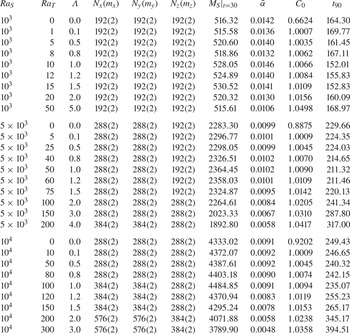
Initially, the velocity is set to zero and the temperature has a vertically linear distribution. The initial concentration field is uniform and equal to a small positive value within the domain to avoid any unphysical negative value during the simulation. A hyperbolic tangent function is applied to introduce a smooth transition between the concentration at the top boundary and the initial value at the interior of the domain. Random perturbations with a magnitude of  $10^{-3}$ are introduced to trigger the convective motions. With these initial conditions, the 3-D simulations are conducted systematically for the parameters stated in figure 1. The details of the numerical settings are summarized in the Appendix. As a validation of our numerical method, we conducted a simulation of RDC at
 ${\textit {Ra}}=10^4$ with the same flow configuration as Pirozzoli et al. (Reference Pirozzoli, De Paoli, Zonta and Soldati2021). By using the same definition of the Nusselt number, our numerical measurements show
 ${\textit {Nu}}=98.44$, which is close to
 $99.84$ given by Pirozzoli et al. (Reference Pirozzoli, De Paoli, Zonta and Soldati2021).
3. Flow structures
In the current simulations, initially the concentration field is unstably stratified only at the top boundary, exactly where the convective motions develop first. Moreover, the extra unstable temperature difference may also affect the evolution of the flow. One may anticipate that, for a weak temperature difference, the flow should be very similar to that without a temperature difference. When the temperature difference is large enough to drive the convective motions, it is very likely that the flow evolution is strongly altered.
This is indeed the case, and we demonstrate this by comparing the two simulations with  ${\textit {Ra}}_T=10$ and
 $300$ for fixed
 ${\textit {Ra}}_S=10^4$. The former case has
 ${\textit {Ra}}_T<{\textit {Ra}}^{cr}_T$ and the latter has
 ${\textit {Ra}}_T>{\textit {Ra}}^{cr}_T$. We first compare the time history of the root-mean-square (r.m.s.) value of the vertical velocity
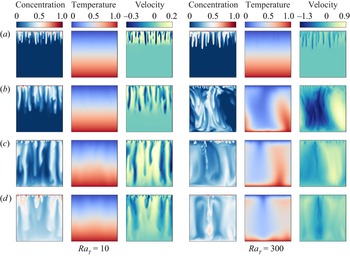
 $u^{rms}_z$ for the two cases, see figure 2. Meanwhile, the concentration, temperature and vertical velocity fields on a vertical plane at four different moments are shown in figure 3. During the initial growth of the flow motions, at approximately
 $t<2.5$, the increase of
 $u^{rms}_z$ is very similar between the two cases. At this stage, the flow motions are mainly driven by the large concentration gradient near the top boundary, and the dominant structures are the concentration fingers originated from the top plate, as shown in figure 3(a). The fingers extend to similar height for the two cases and both temperature fields are nearly undisturbed. The vertical velocity fields have similar structures to concentration fingers.
The time history of the r.m.s. of the vertical velocity  $u_z$ for two cases with
 ${\textit {Ra}}_T=10$ and
 ${\textit {Ra}}_T=300$ and fixed
 ${\textit {Ra}}_S=10^4$. The four dashed vertical lines mark the time at which the slices are shown in figure 3.

The concentration, temperature and vertical velocity contours on a vertical slice at different moments. Panels (a–d) show  $t=2.0$,
 $5.0$,
 $12.0$, and
 $20.0$, respectively. The three columns on the left are for the case with
 ${\textit {Ra}}_T=10$, and the three columns on the right for the case with
 ${\textit {Ra}}_T=300$. For both cases
 ${\textit {Ra}}_S=10^4$.

As the flow further develops, the influence of the temperature gradient begins to arise, see figure 3(b–d). For the case with  ${\textit {Ra}}_T=10$, finger structures continue to grow downward and reach the bottom boundary. The temperature field only exhibits weak oscillations which have a similar characteristic width as the fingers, indicating that they are induced by the fingering motion. The vertical velocity field shows that downwelling fingers move fastest. Fingers randomly distribute in the horizontal direction. Meanwhile, for the case with
 ${\textit {Ra}}_T=300$, which is considerably larger than
 ${\textit {Ra}}^{cr}_T=4{\rm \pi} ^2$, the temperature difference drives the large-scale convection rolls which appear later than the fingers driven by the concentration gradient. The large-scale rolls cause the peak at
 $t=5$ in the time history of
 $u^{rms}_z$ shown in figure 2. The finger structures are also strongly modulated by these large-scale roles: fingers cluster into the descending currents generated by the convection rolls and are suppressed by the upwelling currents. Therefore, inhomogeneity develops in the horizontal distributions of concentration fingers. The large-scale rolls also have larger vertical velocity compared with finger structures, which is in agreement with the larger
 $u^{rms}_z$ for
 ${\textit {Ra}}_T=300$ after the initial growth in figure 2.
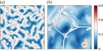
This inhomogeneity can be clearly seen in the concentration contours on the horizontal slice  $z=0.9$ and at the time
 $t=10$, as shown in figure 4. Panel (a) displays the concentration field for the case with
 ${\textit {Ra}}_T=10$, and all the high concentration patches are the cross-sections of finger structures. Indeed they are distributed randomly on the horizontal plane. While in (b), for the case with
 ${\textit {Ra}}_T=300$, the high concentration regions follow long and thin filaments, where the downwelling currents of the large-scale rolls are located.
The concentration contours on the horizontal slice  $z=0.9$ at the time
 $t=10$ for the cases with(a)
 ${\textit {Ra}}_T=10$ and (b)
 ${\textit {Ra}}_T=300$. For both cases
 ${\textit {Ra}}_S=10^4$.

Figure 5 further demonstrates the influence of the temperature difference by comparing the temporal evolution of the horizontally averaged concentration and the temperature profiles for the same two cases. For the case with smaller  ${\textit {Ra}}_T=10$, the mean temperature profiles are almost linear during the entire simulation. As the finger structures develop, a high concentration region extends downwards. Interestingly, as the fingers reach the bottom boundary, they directly transport concentration to the bottom region where the mean concentration rises before the bulk region. This phenomenon appears at around
 $t=10$ as shown in figure 5(a). As the concentration accumulates at the bottom, the density difference across the domain decreases and the flow motions become weaker, corresponding to the gradually decreasing
 $u^{rms}_z$ shown in figure 2; see the blue line after
 $t>10$.
The time evolution of the spatially averaged profiles for the cases with (a,b)  ${\textit {Ra}}_T=10$ and(c,d)
 ${\textit {Ra}}_T=300$. For both cases
 ${\textit {Ra}}_S=10^4$. Panels (a,c) show the averaged concentration profiles and (b,d) the averaged temperature profiles.

For the other case with  ${\textit {Ra}}_T=300$, the large-scale rolls driven by the temperature field appear at approximately
 $t=5$, and figure 5(d) reveals that the temperature field quickly becomes homogeneous afterwards. The large-scale rolls quickly transport the high concentration fluid to the lower part of the domain, and the low concentration fluid to the upper part; see the profiles just after
 $t=5$ shown in figure 5(c). These overturns in mean profiles are clearly the footprint of the large-scale convection rolls induced by the temperature difference. The overturn happens several times and then the mean concentration distribution is homogenized in the bulk.
To quantitatively reveal the horizontal length of the flow structures, we calculate the autocorrelation function of concentration field as
 \begin{equation} {C_S\left(\delta r\right)=\frac{\left\langle\left[S(\boldsymbol{r})-\mu_S\right] \left[S\left(\boldsymbol{r}+\boldsymbol{\delta r}\right)-\mu_S\right]\right\rangle_h}{\sigma_S^2},} \end{equation}
where  $\mu _S$ and
 $\sigma _S$ are the mean and standard deviation of concentration, and
 $\langle ~\rangle _h$ stands for the average over a horizontal slice during the time period
 $t=20\unicode{x2013}30$;
 $\boldsymbol {r}=(x,y)$ is the position vector within the horizontal plane;
 $\boldsymbol {\delta r}$ is the separation vector with
 $\delta r=|\boldsymbol {\delta r}|$. The horizontal plane at the height where
 $u_z^{rms}$ is the largest is used. Then, the typical horizontal length
 $\lambda _h$ can be extracted as the separation
 $\delta r$ at the first minimum of
 $C_S(\delta r)$. Figure 6(a) displays the 1-D autocorrelation function
 $C_S(\delta r)$ for all the cases with
 ${\textit {Ra}}_S=10^4$, and the dependence of
 $\lambda _h$ on the thermal Rayleigh number is plotted in figure 6(b). It is evident that
 $\lambda _h$ first increases with
 ${\textit {Ra}}_T$ as the dominant structures change from fingers to convection rolls, and then does not change much as
 ${\textit {Ra}}_T$ further increases.
(a) The autocorrelation function  $C_S(\delta _r)$ and (b) the variation of horizontal length scale vs the thermal Rayleigh number for fixed
 ${\textit {Ra}}_S=10^4$.

4. Transport properties
4.1. Evolution of Nusselt numbers
One of the key questions for the current flow is the rate at which the dissolved CO $_2$ is transferred downwards. Since the bottom boundary is impermeable for the CO
 $_2$ concentration, the concentration flux is measured at the top boundary as, by the non-dimensional quantities,
 \begin{equation}
{\textit{Nu}}_S(t) = \langle \partial_z
S|_{z=1} \rangle_h =\int_0^1\int_0^1
\partial_z S|_{z=1} \mathrm{d}x \,\mathrm{d}y.
\end{equation}
Meanwhile, the heat flux is calculated as the mean of the fluxes through the top and bottom boundaries as
 \begin{equation}
{\textit{Nu}}_T(t) = \tfrac{1}{2} (\langle
\partial_z T |_{z=1} \rangle_h +
\langle\partial_z T|_{z=0}
\rangle_h).
\end{equation}
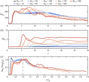
In figure 7 we plot the complete time evolution of  ${\textit {Nu}}_S(t)$ and
 ${\textit {Nu}}_T(t)$ for fixed
 ${\textit {Ra}}_S=10^4$ and increasing
 ${\textit {Ra}}_T$. For the case with
 ${\textit {Ra}}_T=0$, i.e. without a temperature difference, the time history of
 ${\textit {Nu}}_S(t)$ is very similar to those reported in Hewitt et al. (Reference Hewitt, Neufeld and Lister2013). Initially, the concentration flux is dominated by the diffusion process and remains at a small value. When the convective motions start to develop at the top boundary at
 $t\approx 1$,
 ${\textit {Nu}}_S$ increases exponentially and reaches a maximum at approximately
 $t=2.5$. After this peak
 ${\textit {Nu}}_S$ decreases and then maintains a nearly constant value until
 $t=15$, and the flow is in an intermediate quasi-steady state. Then,
 ${\textit {Nu}}_S$ continues to slowly decrease until the end of the simulation at
 $t=30$. This last stage with decreasing
 ${\textit {Nu}}_S$ is identified as the shutdown process by Hewitt et al. (Reference Hewitt, Neufeld and Lister2013).
Temporal evolution of (a) concentration Nusselt number  ${\textit {Nu}}_S(t)$, (b) temperature Nusselt number
 ${\textit {Nu}}_T(t)$ and (c) normalized concentration Nusselt number for
 ${\textit {Ra}}_S=10^4$. Colours from cold to warm correspond to increasing
 ${\textit {Ra}}_T$.

When the temperature difference is introduced across a layer of porous medium, different evolution behaviours are observed for different  ${\textit {Ra}}_T$. For small
 ${\textit {Ra}}_T$, the time history of
 ${\textit {Nu}}_S$ does not change much compared with the case without a temperature difference, which is expected. The value of
 ${\textit {Nu}}_T$ increases slightly from unity when the convective motions induced by the concentration field become apparent. For large
 ${\textit {Ra}}_T$, the temperature difference alone is strong enough to drive convective motions, and
 ${\textit {Nu}}_T$ can be higher than unity after a certain time. The value of
 ${\textit {Nu}}_T$ first quickly increases and then oscillates around a final value. The initial increase of
 ${\textit {Nu}}_T$ happens earlier and the final value becomes larger for higher
 ${\textit {Ra}}_T$. This second scenario occurs when
 ${\textit {Ra}}_T$ is considerably larger than the critical value
 ${\textit {Ra}}^{cr}_T$, which we refer to as the high
 ${\textit {Ra}}_T$ cases.
The comparison between the time history of  ${\textit {Nu}}_S$ and that of
 ${\textit {Nu}}_T$ reveals that, for the high
 ${\textit {Ra}}_T$ cases,
 ${\textit {Nu}}_S$ starts to increase at an earlier time than
 ${\textit {Nu}}_T$ does. Together with the flow evolution shown in the previous section, one discovers that the initial increase of
 ${\textit {Nu}}_S$ corresponds to the finger structures driven by the concentration gradient near the top boundary, while the initial increase of
 ${\textit {Nu}}_T$ happens roughly at the same time as when the large-scale rolls driven by the temperature difference emerge. The appearance of these large-scale rolls also destroys the quasi-steady state which exists in the low
 ${\textit {Ra}}_T$ cases and the flow directly enters the final shutdown process, which will be further discussed in § 4.2.
The above discussions suggest that the large-scale rolls driven by the temperature difference have two opposite effects on the concentration transport. At the early stage, the appearance of large-scale rolls greatly enhances the downward transport rate of the concentration field. At the later stage, however, the non-dimensional concentration flux is suppressed for the cases with high  ${\textit {Ra}}_T$. This latter effect is due to the fact that the upwelling currents of the large-scale rolls can prevent the descent of high concentration fingers near the top boundary, which can be observed in figure 3(c,d). Moreover, the larger concentration flux carried by the downwelling currents of large-scale rolls accelerates the accumulation of high concentration at the bottom region and the transition towards the shutdown process.
During the final shutdown stage, the time history of  ${\textit {Nu}}_S$ exhibits self-similarity for different
 ${\textit {Ra}}_T$. To demonstrate this, we normalize the time
 $t$ by
 $t_m$ when
 ${\textit {Nu}}_T$ reaches the first maximum, and
 ${\textit {Nu}}_S$ by the value
 ${\textit {Nu}}_S(t_m)$. The rescaled plot is shown in figure 7(c). One observes that all the curves for different
 ${\textit {Ra}}_T$ collapse to certain extent for the range
 $t/t_m>1$. This enables us to develop a theoretical model for the shutdown stage as described in the following subsection.
As a final remark on the evolution of the fluxes, we plot the time history of  ${\textit {Nu}}_S$ and
 ${\textit {Nu}}_T$ for three cases with fixed
 $\varLambda =2$ and increasing
 ${\textit {Ra}}_S$ in figure 8. The thermal Rayleigh number
 ${\textit {Ra}}_T$ then increases accordingly. For the smallest
 ${\textit {Ra}}_S=10^3$,
 ${\textit {Ra}}_T={\textit {Ra}}_S\varLambda /{\textit {Le}}=20$ which is below
 ${\textit {Ra}}_T^{cr}$ and the temperature gradient shows a very minor effect on the fluxes. As
 ${\textit {Ra}}_T$ becomes higher than
 ${\textit {Ra}}_T^{cr}$ for the two cases with
 ${\textit {Ra}}_S=5\times 10^3$ and
 $10^4$, similar behaviours are observed as those shown in figure 7 with large
 ${\textit {Ra}}_T$. For larger
 ${\textit {Ra}}_T$, the large-scale convection rolls develop within a shorter time period and
 ${\textit {Nu}}_T$ starts to rise earlier, which causes the faster transition of the flow into the final shutdown stage.
The time evolution of fluxes for three cases with fixed  $\varLambda =2$ and increasing
 ${\textit {Ra}}_S$.

4.2. A theoretical model for the shutdown stage
Following the procedure in Hewitt et al. (Reference Hewitt, Neufeld and Lister2013), we present a theoretical model to describe the temporal variations of concentration flux and volume averaged concentration during the final shutdown stage. We define the instantaneous volume averaged concentration as
 \begin{equation} \mathcal{S}(t)=\int_0^1 \int_0^1 \int_0^1 S(x,y,z,t)\,{{\rm d}x}\,{{\rm d}y}\,{\rm d} z. \end{equation}
At any given time  $t$, if we integrate the concentration equation (2.3d) over the entire domain, then by using the boundary conditions and the definition of
 ${\textit {Nu}}_S(t)$ it is easy to obtain
 \begin{equation} \frac{{\rm d} \mathcal{S}}{{\rm d} t} =\frac{1}{{\textit{Ra}}_{S}} {\textit{Nu}}_S(t). \end{equation}
The above ordinary differential equation can be closed by an appropriate relation between  ${\textit {Nu}}_S(t)$ and
 $\mathcal {S}(t)$. Similar to Hewitt et al. (Reference Hewitt, Neufeld and Lister2013), we use the relation between the Nusselt number and the Rayleigh number for the convection in a porous medium driven by a constant concentration difference across the layer. Since the current flow is constantly evolving, the instantaneous Nusselt and Rayleigh numbers must be defined properly. At any given time, the actual concentration difference, which provides part of the driving force, can be approximated as
 $1-\mathcal {S}(t)$, while the constant temperature difference also contributes to the driving force of the system. Then an effective total Rayleigh number, which measures the strength of the actual driving force, can be defined as
 \begin{equation} {\textit{Ra}}_e(t) = {\textit{Ra}}_S[1-\mathcal{S}(t)]+{\textit{Ra}}_T. \end{equation}
The effective Nusselt number at any time, which should be rescaled by the actual concentration difference, can be calculated as
 \begin{equation} {\textit{Nu}}_e(t)=\frac{{\textit{Nu}}_S(t)}{1-\mathcal{S}(t)}. \end{equation}
Then, as suggested by Hewitt et al. (Reference Hewitt, Neufeld and Lister2013) and Hewitt et al. (Reference Hewitt, Neufeld and Lister2014), a linear scaling can be applied to the relation between the effective Nusselt number and the effective Rayleigh number as
 \begin{equation} {\textit{Nu}}_e(t)=4\alpha {\textit{Ra}}_e(t), \end{equation}
where  $\alpha$ is a scaling coefficient and will be discussed later.
With the help of (4.6), (4.5) and (4.7), equation (4.4) can be closed and gives
 \begin{equation} \frac{{\rm d}\mathcal{S}}{{\rm d} t} =\frac{1-\mathcal{S}}{Ra_{S}} 4\alpha\left[ Ra_S (1-\mathcal{S})+Ra_T\right]. \end{equation}
The solution of the above equations can be readily obtained. For the case without a thermal gradient, for  ${\textit {Ra}}_T=0$, the solution reads
 \begin{equation} \mathcal{S}(t)= 1-\left(C_0+4\alpha t\right)^{{-}1}, \end{equation}
which is the same as that given in Hewitt et al. (Reference Hewitt, Neufeld and Lister2013). Here,  $C_0$ is some integral constant and will be determined from the simulation results. The corresponding Nusselt number is
 \begin{equation} {\textit{Nu}}_S(t)=4\alpha {\textit{Ra}}_S\left(C_0+4\alpha t\right)^{{-}2}. \end{equation}
When  ${\textit {Ra}}_T>0$, the solution takes a more complex form as
 \begin{equation} \mathcal{S}(t)=1-\frac{{\textit{Ra}}_T}{{\textit{Ra}}_S}\left[C_0 \exp\left(\frac{4\alpha {\textit{Ra}}_T t}{{\textit{Ra}}_S}\right)-1\right]^{{-}1}. \end{equation}
And the Nusselt number is
 \begin{align} {\textit{Nu}}_S(t)= 4\alpha \frac{{\textit{Ra}}_T^2}{{\textit{Ra}}_S}\left[C_0 \exp\left(\frac{4\alpha {\textit{Ra}}_T t}{{\textit{Ra}}_S} \right)-1\right]^{{-}1} \left[ \left(C_0 \exp\left(\frac{4\alpha {\textit{Ra}}_T t}{{\textit{Ra}}_S}\right)-1\right)^{{-}1}+1\right]. \end{align}
The above solutions contain two parameters, namely  $\alpha$ and
 $C_0$, which need to be determined from the numerical results.
We first look at the coefficient  $\alpha$. Note that the linear scaling (4.7) is adopted from the RDC driven by a constant temperature difference. Here, the value of
 $\alpha$ will also be affected by the strength of thermal difference. In order to determine the value of
 $\alpha$, one notices that, by using the expressions for
 $\mathcal {S}(t)$ and
 ${\textit {Nu}}_S(t)$,
 \begin{equation} \alpha=\frac{{\textit{Nu}}_S}{4(1-\mathcal{S})\left[{\textit{Ra}}_S (1-\mathcal{S})+{\textit{Ra}}_T\right]}. \end{equation}
The time variations of  $\alpha$ for all the cases with
 ${\textit {Ra}}_S=10^4$ are shown in figure 9. For all cases
 $\alpha$ is almost constant during the last ten time units, especially for the cases with small
 ${\textit {Ra}}_T$. We therefore calculate the mean
 $\bar {\alpha }$ over the time period
 $20 \le t \le 30$. Then the value of
 $C_0$ is then determined by fitting the curve of
 $\mathcal {S}(t)$ over the same time period. The values of
 $\bar {\alpha }$ and
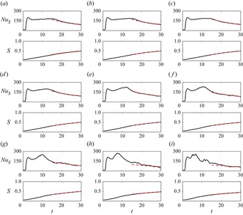
 $C_0$ are summarized in table 1. In figure 10 we compare the theoretical model with the numerical results for all the cases with
 ${\textit {Ra}}_S=10^4$. The agreement between the model and the numerical curves is very good, especially during the final time period. Numerical results also indicate that a similar agreement is achieved for the cases with
 ${\textit {Ra}}_S=10^3$ and
 $5\times 10^3$.
Time evolution of  $\alpha$ for all the cases with
 ${\textit {Ra}}_S=10^4$.

Solid lines show the variations of concentration Nusselt number  ${\textit {Nu}}_S(t)$ and the volume averaged concentration
 $\mathcal {S}(t)$ vs time, while the dashed lines are the predictions of model (4.9) and (4.11). Panels (a–i) show
 ${\textit {Ra}}_T=0$,
 $10$,
 $50$,
 $80$,
 $100$,
 $120$,
 $150$,
 $200$ and
 $300$, respectively;
 ${\textit {Ra}}_S=10^4$ for all cases.

Summary of simulations. Columns from left to right are the concentration Rayleigh number, thermal Rayleigh number, density ratio, resolutions in the  $x$-axis,
 $y$-axis,
 $z$-axis (with refinement factors for multiple resolutions), total CO
 $_2$ transferred to the domain at the end time of the simulations, averaged values of
 $\alpha$ from
 $t=20$ to
 $30$, fitted integral coefficient, predicted time to reach
 $\mathcal {S}=0.9$.

The variation of  $\bar {\alpha }$ vs
 ${\textit {Ra}}_T$ is plotted in figure 11 for all cases. At small
 ${\textit {Ra}}_T$,
 $\bar {\alpha }$ is nearly independent of
 ${\textit {Ra}}_T$ but decreases as
 ${\textit {Ra}}_S$ increases. For the two higher
 ${\textit {Ra}}_S$ considered here,
 $\bar {\alpha }$ is very close to those reported in Hewitt et al. (Reference Hewitt, Neufeld and Lister2014). When
 ${\textit {Ra}}_T$ is large enough,
 $\bar {\alpha }$ exhibits a consistent dependence on
 ${\textit {Ra}}_T$ for all the cases with different
 ${\textit {Ra}}_S$, gradually decreasing with
 ${\textit {Ra}}_T$. For the highest
 ${\textit {Ra}}_T=300$,
 $\bar {\alpha }$ is below
 $0.005$. One possible explanation for the decrease of
 $\bar {\alpha }$ can be attributed to the difference between the flow morphology at small
 ${\textit {Ra}}_T$ and that at large
 ${\textit {Ra}}_T$. As shown in figures 3 and 4, at small
 ${\textit {Ra}}_T$ the concentration fingers develop over the whole domain and the flow is fully three-dimensional. While at large
 ${\textit {Ra}}_T$, fingers mainly develop in the region the downwelling currents induced by the large-scale convection rolls driven by the thermal gradient. That is, the flow morphology is more similar to the quasi-2-D flow over the narrow sheet-like region of downwelling currents. Previous studies suggest that the scaling coefficient
 $\alpha$ takes different values for 2-D and 3-D flows. For 3-D flows, Hewitt et al. (Reference Hewitt, Neufeld and Lister2014) suggests
 $\alpha \approx 0.0096$, while for 2-D flows
 $\alpha$ is smaller and around
 $0.0069$ (Hewitt, Neufeld & Lister Reference Hewitt, Neufeld and Lister2012). These values are very similar to those at small
 ${\textit {Ra}}_T$ and large
 ${\textit {Ra}}_T$ in the current flow.
The coefficient  $\bar {\alpha }$ vs the thermal Rayleigh number
 ${\textit {Ra}}_T$ for all cases.

4.3. Dissolved carbon dioxide
In the previous section we discussed the evolution of flow structures and fluxes. In this subsection we focus on the total carbon dioxide which is transported during the entire simulation time. The total CO $_2$ transferred through the top boundary into the domain at given time
 $t$ can be calculated by the following integration:
 \begin{equation} M_S(t) = \int_0^t {\textit{Nu}}_S(\tau)\,{\rm d}\tau. \end{equation}
Figure 12(a) shows  $M_S(t)$ for all cases with
 ${\textit {Ra}}_S=10^4$;
 $M_S(t)$ exhibits non-monotonic variations as
 ${\textit {Ra}}_T$ increases. Let
 $M^0_S(t)$ denote the case with
 ${\textit {Ra}}_T=0$, then for small
 ${\textit {Ra}}_T$, namely
 ${\textit {Ra}}_T \le 100$ in the current study,
 $M_S(t)$ is larger than
 $M^0_S(t)$ during the entire simulation time
 $0< t<30$. When
 ${\textit {Ra}}_T$ is high enough, first
 $M_S(t)$ is larger than
 $M^0_S(t)$ and then smaller than
 $M^0_S(t)$ at the final stage. These variations with increasing
 ${\textit {Ra}}_T$ can be seen more clearly in figure 12(b) where the same functions are normalized by
 $M^0_S(t)$. The transition from
 $M_S>M^0_S$ to
 $M_S< M^0_S$ occurs at later time as
 ${\textit {Ra}}_T$ becomes smaller. Due to the limitation of the current simulation time, we do not observe this transition for
 ${\textit {Ra}}_T\le 100$. For larger
 ${\textit {Ra}}_T$, there exist two peaks in the time history of
 $M_S/M_S^0$. Comparisons with the time history of the two Nusselt numbers shown in figure 7 reveal that the first peak of
 $M_S/M^0_S$ for different
 ${\textit {Ra}}_T$ occurs at almost the same time of around
 $t=2.5$, which corresponds to the end of the exponential growth of
 ${\textit {Nu}}_S$. During this initial period, the temperature field does not have significant effects on the fluxes, and the flow is mainly driven by the concentration field. The amplitudes of first peaks vary for different
 ${\textit {Ra}}_T$ because of different initial perturbations before the rapid increase of
 ${\textit {Nu}}_S$. The second peak is noticeable for cases with
 ${\textit {Ra}}_T \ge 100$ in figures 7(a) and 12(b). For each
 ${\textit {Ra}}_T$ the second peak of
 $M_S/M^0_S$ is related to the second rise of
 ${\textit {Nu}}_S$. At this stage,
 ${\textit {Nu}}_T$ is evidently larger than unity at higher
 ${\textit {Ra}}_T$. The presence of large-scale rolls changes the instantaneous concentration flux at the top boundary, and therefore the total transferred CO
 $_2$. It takes less time for the flow to form these rolls at larger
 ${\textit {Ra}}_T$, which corresponds to an earlier occurrence of the second peak of
 $M_S/M^0_S$.
(a) The accumulative transfer of CO $_2$ as the function of time for the cases with
 ${\textit {Ra}}_S=10^4$. (b) The same functions normalized by that of the case with
 ${\textit {Ra}}_T=0$. Here,
 ${\textit {Ra}}_T$ increases as the line colour changes from blue to red.

We then look at the total CO $_2$ transported into the domain at the end of the simulations. Figure 13 displays the ratio
 $M_S/M^0_S$ at
 $t=30$ vs
 ${\textit {Ra}}_T$ and
 $\varLambda$ for all simulated cases. For all three concentration Rayleigh numbers, the ratio first increases then decreases with
 $\varLambda$, see figure 13(b). For the smallest
 ${\textit {Ra}}_S=10^3$, the largest thermal Rayleigh number
 ${\textit {Ra}}_T=50$ is only slightly higher than the critical value
 ${\textit {Ra}}_T^{cr}$ and the convective motions driven by the thermal gradient are not strong. Still, the additional temperature difference across the domain has noticeable effects on the accumulative transfer of CO
 $_2$. As
 ${\textit {Ra}}_S$ increases, the ratio
 $M_S/M^0_S$ at
 $t=30$ reaches the peak value at larger
 ${\textit {Ra}}_T$. Moreover, when
 ${\textit {Ra}}_T$ is large enough, the ratio drops below unity, indicating that the total CO
 $_2$ transported downwards at
 $t=30$ is less than that without the presence of a temperature difference. For the case with
 ${\textit {Ra}}_S=5\times 10^3$ and
 ${\textit {Ra}}_T=200$, the total amount of CO
 $_2$ transferred into the domain at
 $t=30$ can be reduced by over
 $17\,\%$ compared with the case with
 ${\textit {Ra}}_T=0$. Interestingly, if the ratio
 $M_S/M_S^0$ at
 $t=30$ is plotted against the density ratio
 $\varLambda$, see figure 13(b), one observes that the ratio reaches the maximum at around
 $\varLambda =1$ for all three
 ${\textit {Ra}}_S$. The maximal increment in
 $M_S$ induced by the temperature difference is over
 $3\,\%$ for the two larger
 ${\textit {Ra}}_S$. This non-monotonic trend can be understood as follows. Two opposite effects are introduced by the unstable temperature gradient. On one hand, the vertical flow motions are stronger due to the extra buoyancy force of the thermal field. On the other hand, the concentration fingers are clustered by the large-scale rolls driven by the thermal field. The former will enhance the downward transport while the latter will suppress the transport because of the reduction of the horizontal area with larger concentration.
The ratio  $M_S/M^0_S$ at
 $t=30$, i.e. the end of the simulation, vs (a) the thermal Rayleigh number
 ${\textit {Ra}}_T$ and (b) the density ratio
 $\varLambda$.

To quantitatively demonstrate these two effects, we employ the r.m.s. value  $u^{rms}_z$ of the vertical velocity and the total area
 $\varOmega$ of the regions where
 $S'>S_{std}$ and
 $u_z'<-u^{std}_z$. Here,
 $S'$ and
 $u_z'$ are the deviations from the horizontally averaged concentration and vertical velocity, while
 $S_{std}$ and
 $u^{std}_z$ are the corresponding standard deviations. The two values
 $u^{rms}_z$ and
 $\varOmega$ are calculated over the horizontal plane at the height with maximal
 $u^{rms}_z$ and then averaged over the time period
 $20\le t \le 30$. In figure 14 we plot the dependence of
 $\overline {u^{rms}_z}$ and
 $\bar {\varOmega }$ on the density ratio
 $\varLambda$ for fixed
 ${\textit {Ra}}_S=10^4$. Clearly,
 $\overline {u^{rms}_z}$ increases with
 $\varLambda$, while
 $\bar {\varOmega }$ decreases. The two curves intersect with each other at some moderate density ratio slightly above unity. Therefore, the maximal
 $M_S/M_S^0$ at moderate density ratio is very likely caused by these two competing effects of the thermal field.
The averaged  $\overline {u^{rms}_z}$ and
 $\bar {\varOmega }$ over the time period
 $20\le t \le 30$. For all cases
 ${\textit {Ra}}_S=10^4$.

For the current flow configuration, the whole domain will eventually have  $\mathcal {S}=1$ when the time approaches infinity. The theoretical model constructed in the previous section can provide some indications about the long-term behaviours of the total dissolved carbon dioxide. By using (4.9) and (4.11) and the coefficients determined from the numerical results, we estimate the time
 $t_{90}$ when
 $\mathcal {S}=0.9$, i.e. where the volume averaged concentration equals to
 $90\,\%$ of the concentration at the top boundary. The values of
 $t_{90}$ are listed in table 1, and their dependence on
 $\varLambda$ is plotted in figure 15. Note that
 $t_{90}$ is in the non-dimensional form. Figure 15 suggests that overall
 $t_{90}$ increases with
 ${\textit {Ra}}_S$. For fixed
 ${\textit {Ra}}_S$, however,
 $t_{90}$ generally first decreases and then increases with
 $\varLambda$ or equivalently
 ${\textit {Ra}}_T$. It reaches the minimum around
 $\varLambda =1$ for all three
 ${\textit {Ra}}_S$ considered here.


4.4. Implications for CO $_2$ sequestration

Above findings reveal that, for high  ${\textit {Ra}}_S$, which is very likely the case in a real geological reservoir, a weak to moderate geothermal gradient may increase the total carbon dioxide transferred into the saline aquifer due to convective dissolution during a certain time period, while a strong geothermal gradient may have the opposite effect. To demonstrate this in the context of a realistic situation, we take a typical geological reservoir with porosity
 $\phi =0.2$, permeability
 $K=1.25\times 10^{-13}\,\mathrm {m}^2$, viscosity
 $\mu =2\times 10^{-4}\,{\rm Pa}\,{\rm s}$, overall thermal diffusivity
 $\kappa _m=10^{-7}\,\mathrm {m}^2\,{\rm s}^{-1}$ and concentration diffusivity
 ${\kappa _S=5\times 10^{-9}\,\mathrm {m}^2\,{\rm s}^{-1}}$. For brine saturated with CO
 $_2$, the density increment is approximately
 $8\,\mathrm {kg}\,{\rm m}^{-3}$. Then a
 $200\,\mathrm {m}$ aquifer will give a concentration Rayleigh number
 ${\textit {Ra}}_S=10^4$ if roughly taking
 $g=10\,\mathrm {m}\,{\rm s}^{-2}$, and the non-dimensional simulation time
 $t=30$ corresponds to approximately
 $760$ years. Assuming a geothermal gradient of
 $50\,^{\circ }\mathrm {C}\,{\rm km}^{-1}$, the temperature difference and thermal Rayleigh number across the aquifer are
 ${\rm \Delta} T=10\,^{\circ }\mathrm {C}$ and
 ${\textit {Ra}}_T=100$ by using
 $\beta _T=8\times 10^{-4}\,\mathrm {K}^{-1}$, respectively. Therefore, under this circumstance, the density ratio is
 $1.0$. For an aquifer with an area of
 $100\,\mathrm {km}^2$, approximately
 $2.4\times 10^6$ tons of extra CO
 $_2$ will be transferred into the aquifer from the perspective of convective dissolution with a geothermal gradient during the time period of
 $760$ years.
Furthermore, our results suggest that the large-scale convection rolls driven by the thermal gradient can strongly alter the horizontal pattern of the finger structures. In actual environments, finger structures mainly happen at the interface region between the supercritical CO $_2$ layer and the brine layer below. However, the large-scale convection rolls may already exist over a layer with much larger thickness and therefore much higher thermal Rayleigh number. Then, the upwelling and downwelling currents of the large-scale rolls can still affect the horizontal distribution of the finger structures, even though the local thermal Rayleigh number across the interface region is much lower. Also, the geothermal gradient may play a non-negligible role in many CO
 $_2$-sequestration sites.
5. Influence of initial conditions
In all the cases discussed above, initially, the temperature has a linear distribution between the top and bottom boundaries and the fluid is at rest. For the cases with a strong temperature difference, large-scale rolls usually appear after the finger structures, and the influences of these structures driven by temperature difference do not show up at the beginning. As an idealized model, such initial conditions are easy to implement. In real underground environments with strong enough geothermal gradients, however, large-scale convective motions should already exist when the supercritical CO $_2$ is injected. Therefore, in this section we investigate the influences of different initial conditions. We take the case with
 ${\textit {Ra}}_S=10^4$ and
 ${\textit {Ra}}_T=100$ as the reference case, and refer to the initially linear temperature distribution and zero velocity as case IC1. In order to mimic the real environment, we rerun the reference case with the following procedure and refer to this new simulation as case IC2. First, a pure thermally driven convection flow is simulated with
 ${\textit {Ra}}_T=100$ until the flow fully develops and the large-scale rolls are present. We take an instantaneous velocity field and corresponding temperature field as the initial conditions, and set the concentration at the top plate as
 $S_{top}$ with
 ${\textit {Ra}}_S=10^4$. The simulation is then run for another
 $30$ non-dimensional time units.
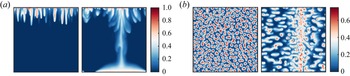
Figure 16 compares the flow fields of cases IC1 and IC2 at the time  $t=2$. At this time the large-scale rolls in case IC1 have not developed yet. Therefore, flow motions are dominated by finger structures, as shown in the left panel of figure 16(a). However, in case IC2, since the large-scale rolls exist at the beginning, at time
 $t=2$, high concentration fluid has already been transported to the bottom of domain by the descending currents of the large-scale rolls, see the right panel of figure 16(a). The concentration fields on the horizontal plane at
 $z=0.9$ also clearly indicate the difference in the horizontal distributions of fingers, as shown in figure 16(b). Fingers are randomly distributed in case IC1 but concentrate at the locations of the downwelling current in case IC2. Note that the downwelling currents form a single sheet which spans the whole width of the domain for the case shown in figure 16(b), while the case in figure 4(b) has multiple sheets intersecting with each other. This difference can be attributed to the different
 ${\textit {Ra}}_T$. The large-scale convection rolls consist of a pair of 2-D rolls for
 ${\textit {Ra}}_T=100$, and several convection cells for
 ${\textit {Ra}}_T=300$.
Flow fields at  $t=2$ for two cases with different initial temperature fields. For both cases
 ${\textit {Ra}}_S=10^4$ and
 ${\textit {Ra}}_T=100$. (a) The concentration contours on a vertical slice. (b) The concentration contours on the horizontal slice at
 $z=0.9$. Within each panel the left image is for the case starting with a linearly distributed temperature field, and the right image is that with a fully developed thermally driven convection field.

The evolution of  ${\textit {Nu}}_S$, which is plotted in figure 17, is also different between the two cases. In the figure we also plot the simulation with
 ${\textit {Ra}}_T=0$ for reference. The intermediate quasi-steady stage in the range
 $5< t<15$ in the case without a temperature difference disappears in case IC1 due to the overlap with the development of large-scale rolls. In case IC2, on the other hand, the large-scale rolls are in their fully developed state at the beginning of the simulation, and a new quasi-steady stage with nearly constant
 ${\textit {Nu}}_S$ exists during the time period
 $3< t<8$. The non-dimensional flux during this stage in case IC2 is higher than the other two cases, and the flow enters the final shutdown process at the earliest time among the three cases. The final shutdown process is similar the
 ${\textit {Nu}}_S$ variation for all cases. It should be pointed out that, although different initial conditions can change the temporal evolution of the fluxes and the dynamics of the flow structures, the final state of the system is only determined by
 ${\textit {Ra}}_T$ since, eventually, the interior fluid will be saturated with carbon dioxide and the convective motions are solely driven by temperature difference.
The temporal evolution of  ${\textit {Nu}}_S$ for three cases with fixed
 ${\textit {Ra}}_S=10^4$. The black line shows the case without a temperature difference, the blue line shows the case with a temperature difference and initially linearly distributed temperature field and the red line shows the case with a temperature difference starting from a fully developed thermally driven convection state, respectively.

6. Conclusions
In summary, we study the influence of the unstable thermal gradient on the convective dissolution of CO $_2$ in 3-D porous media. As a preliminary investigation, we assume all the physical properties are homogeneous and isotropic. Three different concentration Rayleigh numbers are investigated within the range
 $10^3\le {\textit {Ra}}_S\le 10^4$, and for each
 ${\textit {Ra}}_S$ a series of thermal Rayleigh numbers are simulated by using 3-D direct numerical simulation. The explored
 ${\textit {Ra}}_T$ covers the range from below the critical value
 ${\textit {Ra}}_T^{cr}$ to above it. Here,
 ${\textit {Ra}}_T^{cr}$ is the critical value predicted by the linear instability analysis of the porous medium layer experiencing a pure thermal gradient. The simulations are run until
 $30$ non-dimensional time units when the flow is already in the final shutdown process.
When  ${\textit {Ra}}_T$ is smaller than
 ${\textit {Ra}}_T^{cr}$, the temperature difference alone cannot drive convection rolls, and the flow is dominated by finger structures driven by the concentration gradient. The development of finger structures is similar to that without a temperature difference. When
 ${\textit {Ra}}_T$ is large enough to trigger the large-scale rolls, the evolution of finger structures is strongly modulated by these large-scale rolls. Fingers grow faster at the regions of downwelling currents of large-scale rolls, and are suppressed by the upwelling currents. Therefore, the horizontal distribution of fingers is no longer uniformly random but is denser at the downwelling regions of large-scale rolls.
The time evolution of fluxes also exhibits different behaviours for different  ${\textit {Ra}}_T$.A weak temperature difference only has minor effects on the fluxes. The non-dimensional concentration flux quickly increases when the finger structures develop, then is nearly constant during the intermediate quasi-steady stage and finally decreases as the flow enters the shutdown process. For a strong temperature difference, the large-scale rolls enhance the concentration flux at early times and disrupt the quasi-steady stage. The flow enters the final shutdown process faster as
 ${\textit {Ra}}_T$ becomes larger. The flow evolution is self-similar during the shutdown stage, as indicated by the collapse of rescaled
 ${\textit {Nu}}_S$ for different
 ${\textit {Ra}}_T$. As
 ${\textit {Ra}}_T$ increases, the concentration structures shift from fingers to large-scale circulations and the dominant width changes accordingly. When the flow is in the shutdown stage, by assuming a well-mixed internal concentration and applying asymptotic linear scaling in RDC to convective dissolution, we obtain the theoretical predictions of the volume averaged concentration and non-dimensional concentration flux, which are consistent with numerical measurements.
The total amount of CO $_2$ transferred into the domain at the end of simulations shows a non-monotonic dependence on
 ${\textit {Ra}}_T$ for a given
 ${\textit {Ra}}_S$. It first increases and then decreases with
 ${\textit {Ra}}_T$. The maximum is reached at approximately unit density ratio, i.e. the density difference induced by the temperature difference equals that induced by the concentration difference. The implications of the current findings for real CO
 $_2$-sequestration are then discussed for typical saline aquifer properties, and suggest that the influence of the geothermal gradient may not be negligible.
To mimic the real environment where large-scale rolls exist long before CO $_2$ sequestration, we rerun a reference case to examine the influence of initial conditions. Compared with the linear distribution for the initial temperature field, using the fully developed temperature field at the start of simulation can produce a higher quasi-steady stage similar to the case without a thermal gradient. After that the flow also enters the shutdown stage but the flux decays at an earlier time.
Note that the model flow investigated here is different from the double-diffusive convection in porous media, where the temperature and concentration gradients usually have opposite effects on fluid density. The current study opens new directions for the convective dissolution in CO $_2$-sequestration, and more works are needed for future study.
Funding
This work is financially supported by Laoshan Laboratory under the grant no. LSKJ202202000. K.X. is also partially supported by National Natural Science Foundation of China under grant no. 12172010 and China National Petroleum Corporation-Peking University Strategic Cooperation Project of Fundamental Research.
Declaration of interests
The authors report no conflict of interest.
Appendix. Summary of numerical details
The details of the simulations are summarized in table 1. Recall that, for all simulations, the heat capacity ratio and the Lewis number are fixed at  $\sigma =1$ and
 ${\textit {Le}}=100$, respectively.