1 Introduction
Delta-shock is an important class of nonclassical wave for systems of conservation laws. The mathematical feature of the delta-shock is that the delta functions occur in the state variables. Physically, the concentration phenomenon can be described by the delta-shock. Among a large number of models for studying the delta-shock [Reference Danilov and Shelkovich10, Reference Kalisch and Mitrovic17, Reference Keita and Bourgault18, Reference Le Floch20, Reference Pang, Shao, Wen and Ge29, Reference Panov and Shelkovich30, Reference Shen and Sun39, Reference Tan, Zhang and Zheng45], there is a very important one, which is the pressureless Euler system.
This paper is concerned with the pressureless Euler system with zeroth-order terms modelling acoustic generation

where
$\rho $
 and u are density and velocity, respectively, and
$k\rho $
 ,
$\beta \rho $
 and
$k\rho u/2$
 with constant coefficients
$k\neq 0$
 and
$\beta $
 are the zeroth-order acoustic generators. Sound waves are generated by injecting mass and momentum. The coefficient k can quantify the rate of increase (decrease) in the mass of fluid per unit volume. Here,
$k>0$
 indicates that mass is injected (for example, the vaporization of the liquid film increases the mass of the fluid);
$k<0$
 indicates that the mass is extracted (for example, the condensation of the vapour decreases the mass). Additionally,
$\beta $
 is a constant that quantifies the strength of a density-proportional momentum source;
$\beta>0$
 shows that momentum is damped;
$\beta <0$
 shows that momentum is amplified. The term
$k\rho u/2$
 associated with the mass source coefficient k is a velocity-dependent momentum source, where the constant
$k/2$
 quantifies the strength of the momentum source.
We should mention here why the source terms appearing in system (1.1) are selected, especially mass source. It is widely known that in many domains of interest, physical phenomena can be described by balance laws (systems of conservation laws with source terms). For instance, a mass conservation equation with a mass source
$(\Sigma _1(\rho ,u,x,t))$
 for the vapour phase can be expressed by

to reflect the condensation and vaporization processes [Reference Gerber and Kermani11, Reference Wen, Karvounis, Walther, Ding and Yang48], where
$\rho $
 is the vapour (gas) density and u is the vapour (gas) velocity, a positive
$\Sigma _1(\rho ,u,x,t)$
 corresponds to the case of evaporation, while for the condensation process,
$\Sigma _1(\rho ,u,x,t)$
 is negative. Furthermore, as focusing on convective effects, these laws can take the form of a first-order hyperbolic system of partial differential equations, which is composed by a nonlinear time–space divergence balanced by zeroth-order terms. From the physical viewpoint, this corresponds to the balance of convective and acoustic effects by external forces. Inspired by this, these zeroth-order terms
$k\rho $
 ,
$\beta \rho $
 and
$k\rho u/2$
 are chosen.
The system (1.1) can be reduced from the equations of mass and momentum [Reference Clarke and Lowe9, Reference Lowe and Clarke26, Reference Maeda and Colonius27]. The pressureless Euler equations (1.1) with
$k=\beta =0$
 (the homogeneous case) can describe the motion of free particles sticking under collision [Reference Brenier and Grenier3, Reference Weinan, Rykov and Sinai47] and the formation of large-scale structures in the universe [Reference Shandarin and Zeldovich35]. Sheng and Zhang [Reference Sheng and Zhang42] solved the Riemann problems for (1.1) with
$k=\beta =0$
 , and obtained the solutions including delta-shock and vacuum by adopting the vanishing viscosity method. As the friction is taken into account, Shen [Reference Shen36] discussed the Riemann problems for the system (1.1) with
$k=0$
 (the pressureless Euler system with friction) by using variable substitution. Qu et al. [Reference Qu, Yuan and Zhao31] have already pointed out that the pressureless flow is actually a hypersonic limiting flow under suitable scaling. In the high-Mach-number limit, polytropic gas may also be considered as the pressureless flow, provided that the speed of the piston is very large compared with the flow. With the use of the substitution of variables, Li and Wang [Reference Li and Wang25] solved the Riemann problems for the system (1.1) and obtained two kinds of nonself-similar solutions: vacuum solution and delta-shock solution. Furthermore, by using the vanishing viscosity method, the stability of the nonself-similar solutions was established by introducing a time-dependent viscous system.
In recent years, the topic concerning the formation of delta-shocks and vacuum states, and the phenomena of concentration and cavitation in solutions has attracted wide attention from mathematicians and physicists. For instance, Li [Reference Li21], and Chen and Liu [Reference Chen and Liu7, Reference Chen and Liu8] studied the formation of delta-shocks and vacuum states in solutions of the isentropic and nonisentropic Euler equations by introducing the vanishing pressure limit method. Chen and Liu [Reference Chen and Liu7] showed that as the pressure vanishes, the delta-shocks and vacuum of the homogeneous pressureless Euler equations can be formed as the limits of shocks and rarefaction waves of the isentropic Euler equations. Chen and Liu [Reference Chen and Liu8] made a further step to generalize this result to the Euler equations for nonisentropic fluids. Yin and Sheng [Reference Yin and Sheng50, Reference Yin and Sheng51] extended these results to the relativistic Euler equations and relativistic fluid dynamics. Shen and Sun [Reference Shen and Sun38] analysed the formation of delta-shocks and vacuum states in the vanishing pressure limit of Riemann solutions to the perturbed Aw–Rascle model of traffic flow [Reference Aw and Rascle1]. They proved that the Riemann solutions of the Aw–Rascle model of traffic flow with pressure
$p(\rho )=\varepsilon \rho ^\gamma \ (\gamma>1)$
 (they replaced
$\rho p(\rho )$
 with
$p(\rho )$
 ) do not converge to those of pressureless Euler equations as
$\varepsilon \rightarrow 0$
 . To solve this problem, they introduced a perturbed Aw–Rascle model to prove that the delta-shocks and vacuum of the homogeneous pressureless Euler equations can be formed as the limits of shocks and rarefaction waves of the perturbed Aw–Rascle model. Yang and Wang [Reference Yang and Wang49] proved that as the modified Chaplygin gas pressure vanishes, any two-shock solution of the modified Chaplygin gas equations tends to a delta-shock solution of the pressureless Euler equations, and any two-rarefaction-wave solution of the modified Chaplygin gas equations tends to a two-contact-discontinuity solution of the pressureless Euler equations; any two-shock Riemann solution of the modified Chaplygin gas equations tends to a delta-shock solution of the generalized Chaplygin gas equations as the modified Chaplygin gas pressure approaches to the generalized Chaplygin gas pressure. Guo et al. [Reference Guo, Li and Yin12, Reference Guo, Li and Yin13] showed that as the pressure vanishes, the Riemann solutions of the Chaplygin gas equations with friction and the generalized Chaplygin gas equations with friction converge to those of pressureless Euler equations with friction. Li [Reference Li23] constructed two kinds of nonself-similar Riemann solutions including delta-shock for the Chaplygin gas Euler equations modelling acoustic generation and proved that the limits of Riemann solutions to the inhomogeneous Chaplygin gas Euler equations are just the Riemann solutions to the pressureless Euler equations with the same source terms as the Chaplygin gas pressure falls into zero. Zhang [Reference Zhang52] analysed and identified two kinds of occurrence mechanisms on the phenomenon of concentration and the formation of delta-shocks in the flux approximation limit of Riemann solutions to the extended Chaplygin gas equations with Coulomb-like friction [Reference Savage and Hutter33]. Ibrahim et al. [Reference Ibrahim, Liu and Liu16] investigated the formation of the delta-shocks in the Riemann solutions for the isentropic Euler equations with the pressure function
$p(\rho )=\rho ^\gamma ,\ (0<\gamma <1)$
 and proved that the delta-shocks of the homogeneous pressureless Euler equations can be formed as the limits of classical shocks of the isentropic Euler equations as adiabatic index
$\gamma $
 goes to zero. Sheng and Shao [Reference Sheng and Shao41] extended the results to the Euler equations with friction. Shen and Sun [Reference Shen and Sun40] studied the Riemann problem for the isentropic Euler system under the body force with varying gamma law, and analysed the limits of Riemann solutions as the adiabatic exponent tends to one. Sun [Reference Sun44] analysed the concentration and cavitation phenomena of Riemann solutions for the isentropic logarithmic Euler system, and showed that the solution consisting of shocks and the solution composed of rarefaction waves of the logarithmic Euler equations tend to the solution with delta-shock and the solution with vacuum of the homogeneous pressureless Euler equations as the logarithmic pressure goes to zero. Sen and Sekhar [Reference Sen and Raja34] proved that as the logarithmic pressure goes to zero, the Riemann solutions of the isentropic logarithmic Euler system with friction converge to those of pressureless Euler equations with friction.
One can observe from the above analysis that the research with respect to the formation of delta-shocks and vacuum for the pressureless Euler system has mainly focussed on the homogeneous case and the nonhomogeneous case containing only a friction term. Different from the above-mentioned studies, we are interested in exploring the formation of delta-shocks and vacuum states, and the phenomena of concentration and cavitation for the nonhomogeneous pressureless Euler system (1.1) including the mass source term and momentum source term. To this end, we deal with the Riemann problem for the isentropic Euler equations including zeroth-order terms with logarithmic equation of state

subject to the initial data consisting of a pair of constant states

and analyse the limits of solutions as the logarithmic pressure vanishes, where the pressure function
$p(\rho )=A\ln \rho \ (A>0)$
 corresponds to the logarithmic equation of state, which is considered as a perturbation pressure. The logarithmic pressure was introduced in [Reference Chavanis5, Reference Chavanis and Sire6, Reference Odintsov, Oikonomou, Timoshkin, Saridakis and Myrzakulov28] for the dark energy fluid to investigate the dynamical evolution of a late-time universe. Compare and contrast with the several generalized forms of the “Chaplygin gas model” [Reference Bento, Bertolami and Sen2, Reference Chaplygin4], the Euler model with the logarithmic equation of state, which is referred to as the “Logotropic model” [Reference Sun44], offers more interesting cosmological behaviours. Additionally, because the value of the logarithmic function is negative for
$0<\rho <1$
 and positive for
$\rho>1$
 , it can be seen as a transition between the Chaplygin gas (generalized Chaplygin gas) generating the negative pressure and polytropic gas generating the positive pressure. Consequently, it has been introduced as a natural and robust candidate for a new unification of dark matter and dark energy. For more research concerning the homogeneous and nonhomogeneous isentropic Euler system involving friction, please refer to papers [Reference Guo, Sheng and Zhang14, Reference Li22, Reference Li and Wang24, Reference Shen37, Reference Sun43, Reference Wang46].
One can easily observe that under the impact of source terms, the Riemann solutions of (1.2)–(1.3) are nonself-similar. Consequently, it usually leads to additional difficulties and requires new techniques in the study of system (1.2). Here, we solve the Riemann problem for (1.2)–(1.3) through the use of variable substitution. Performing the transformation

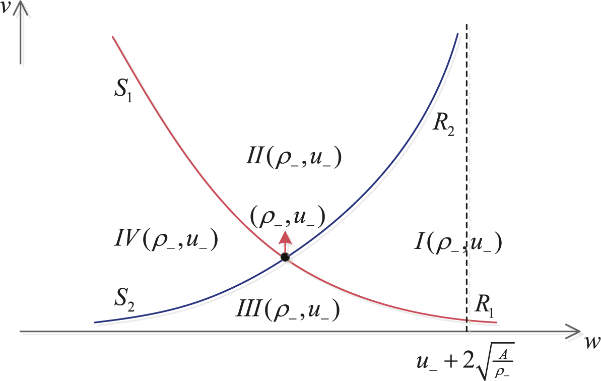
the nonhomogeneous logotropic model (1.2) and initial data (1.3) simplify to the homogeneous conservative system (3.1) and initial data (2.2). The homogeneous conservative system (3.1) is strictly hyperbolic and two characteristic fields are genuinely nonlinear, so the classical elementary waves are formed by rarefactive waves and shocks. The phase plane
$(v,w)$
 is divided into four domains
$I, II, III, IV(\rho _-,u_-)$
 by the classical elementary waves curves. Thanks to the method of phase plane analysis, we construct the solutions with four kinds of different configurations:
$R_1+R_2$
 ,
$S_1+R_2$
 ,
$R_1+S_2$
 ,
$S_1+S_2$
 . Then, four kinds of nonself-similar Riemann solutions of (1.2)–(1.3) are obtained through the use of rarefaction waves and/or shocks connecting two exponential states
$(\rho _\pm e^{kt},(u_\pm -{2\beta }/{k})e^{-{k}t/{2}}+{2\beta }/{k})$
 . Unlike the results in [Reference Sen and Raja34, Reference Sun44], the shapes of all waves are a composite of an exponential function of t and a linear function of t in the
$(x,t)$
 -plane, and all waves propagate at an exponential rate. Additionally, the limit behaviour of the solutions of (3.1) and (2.2) is investigated as
$A\rightarrow 0$
 . Consider the fact that the interior of the regions of
$II(\rho _-,u_-)$
 and
$III(\rho _-,u_-)$
 is empty, so we only need to discuss the limit behaviour of the solutions of (3.1) and (2.2) as
$A\rightarrow 0$
 for the cases
$(\rho _+,u_+)\in I(\rho _-,u_-)\cup IV(\rho _-,u_-)$
 . It is proved that as A drops to zero, the nonself-similar Riemann solution containing two shocks of (3.1) and (2.2) converges to the delta-shock solution of (2.1)–(2.2), and the solution formed by two rarefaction waves of (3.1) with (2.2) tends to the solution containing vacuum of (2.1)–(2.2). Based on the discussions in Section 3, we know that by using the transformation (1.4), the Riemann solutions of (1.2)–(1.3) are obtained by virtue of those of the modified system (3.1) with the same initial data (2.2). Furthermore, because time t, parameters k and
$\beta $
 in the transformation (1.4) are completely independent of the parameter A, it can be asserted that the Riemann solutions of (1.2)–(1.3) being nonself-similar tend to those of (1.1) with (1.3) as A falls to zero.
This paper is organized into five sections. In Section 2, we review the solutions for (1.1) with (1.3). In Section 3, the Riemann solutions of (1.2)–(1.3) are constructed with the use of the substitution of variables. Section 4 proves that in the limits of
$A\rightarrow 0$
 , the nonself-similar solutions of (1.2)–(1.3) tend to the corresponding ones of (1.1) with (1.3). Section 5 gives the conclusion.
2 Riemann solutions of nonhomogeneous zero-pressure Euler system modelling acoustic generation
This section constructs the solutions of the pressureless Euler equations including zeroth-order terms (1.1) with Riemann initial data (1.3). A more detailed discussion can be found in [Reference Li and Wang25].
Under the transformation (1.4), (1.1) and (1.3) simplify to

and

The modified homogeneous system (2.1) has a double eigenvalue

which shows that the system (2.1) is nonstrictly hyperbolic, and
$\lambda $
 is linearly degenerate because the corresponding right eigenvector is
$\overrightarrow {r}=(1,0)^T$
 satisfying
$\nabla \lambda \cdot \overrightarrow {r}\equiv 0$
 .
Let
$\sigma (t)=x'(t)$
 be the speed of a bounded discontinuity
$x=x(t)$
 . Then, the Rankine–Hugoniot [Reference Hugoniot15, Reference Rankine32] condition is

where
$[v]=\rho _--v$
 , and so forth. We eliminate the discontinuity speed,
$\sigma (t)$
 , from (2.3) to get the contact discontinuity

The left state
$(\rho _-,u_-)$
 can be connected with the right state
$(\rho _+,u_+)$
 by a contact discontinuity J, provided that
$u_-=u_+$
 .
If
$u_-<u_+$
 , the Riemann solution of (2.1)–(2.2) is composed of a vacuum state (denoted by Vac) and two contact discontinuities connecting two constant states
$(\rho _\pm ,u_\pm )$
 . The solution can be written as

where

If
$u_->u_+$
 , the Riemann solution with delta-shock can be constructed. To define the solution with delta-shock, the weighted delta function
$\varpi (s)\delta _S$
 (
$\varpi (s)$
 is the weight) supported on a smooth curve
$S=\{(x(s),t(s))\mid c\leq s\leq d\}$
 is defined by

for any test function
$\phi (x,t)\in C^\infty _0((-\infty ,+\infty )\times [0,+\infty ))$
 .
Definition 2.1. A pair
$(v,w)$
 is said to be a delta-shock type solution of (2.1) in the sense of distributions, provided that there exist a smooth curve S and a weight
$\varpi \in C^1(S)$
 such that v and w are represented in the following form:

where
$(v_l,w_l)(x,t)$
 and
$(v_r,w_r)(x,t)$
 are piecewise smooth solutions of the system (2.1), the Heaviside step function
$H(x)$
 takes value zero for negative arguments
$x<0$
 and one for positive arguments
$x>0$
 , and it satisfies

for all test functions
$\phi \in C_{0}^{\infty }((-\infty ,+\infty )\times [0,+\infty ))$
 , where

Under Definition 2.1, the solution can be written as

where the location
$x(t)$
 , the weight
$\varpi (t)$
 and the assignment of w on the discontinuity
$w_\delta $
 satisfy the generalized Rankine–Hugoniot [Reference Hugoniot15, Reference Rankine32] relation

and the entropy condition

with
$[v]=\rho _--\rho _+$
 the jump of v across the discontinuity. Solving (2.4) with initial condition
$x(0)=\varpi (0)=0$
 provides

where
$ w_\delta =({\sqrt {\rho _-}u_-+\sqrt {\rho _+}u_+})/({\sqrt {\rho _-}+\sqrt {\rho _+}}). $

Based on the above analysis, two kinds of Riemann solutions involving delta-shock and vacuum for the nonhomogeneous pressureless Euler system (1.1) with initial data (1.3) can be given by virtue of the transformation (1.4).
When
$u_-<u_+$
 , the Riemann solution including vacuum of (1.1) and (1.3) is expressed as

When
$u_->u_+$
 , the Riemann solution with delta-shock of (1.1) and (1.3) is represented as

in which
$x(t)$
 ,
$w_\delta $
 and
$\varpi (t)$
 are given by (2.5).
3 Riemann solutions for (1.2)–(1.3)
3.1 Riemann solutions for the modified homogeneous system (3.1)
In this subsection, we change the original system (1.2) into a homogeneous system through a suitable transformation and construct the Riemann solutions. Under the transformation (1.4), the original logarithmic model (1.2) and initial data (1.3) become the homogeneous conservative system

and initial data (2.2), respectively.
The matrix form of (3.1) is given by

where

Two eigenvalues of (3.1) are real and distinct, with

which shows that (3.1) is strictly hyperbolic. The corresponding right eigenvectors are found to be

Since

the
$\lambda _1$
 -characteristic field and the
$\lambda _2$
 -characteristic field are genuinely nonlinear.
The Riemann invariants associated with the
$\lambda _1$
 -characteristic field and
$\lambda _2$
 -characteristic field are

which satisfy the equation
$\nabla Q_i\cdot \overrightarrow {r}_i=0$
 . It should be noted that Riemann invariants remain constant across the rarefaction waves, and the characteristic speeds of rarefaction waves starting from
$(\rho _-,u_-)$
 increase from left to right, that is,
$\lambda _i(\rho _-,u_-)< \lambda _i(v,w)$
 .
With the help of (3.2), the
$1$
 -rarefaction wave
$R_1(\rho _-,u_-)$
 is found to be

Using the second equation of (3.3), we take the derivative of w with respect to v to get

which indicates that the
$1$
 -rarefaction wave curve is monotonically decreasing and convex in the
$(v,w)$
 phase plane. Moreover, we have
${\lim \limits _{v\rightarrow 0} w {\kern-1pt}={\kern-1pt}u_--2\sqrt {{A}/{\rho _-}}{\kern-1pt}+{\kern-1pt}2\sqrt {{A}/{v}}{\kern-1pt}={\kern-1pt}+\infty }$
 , which demonstrates that the w-axis is the asymptotic line of the
$1$
 -rarefaction wave curve.
Analogously, the
$2$
 -rarefaction wave
$R_2(\rho _-,u_-)$
 is

By means of the second equation of (3.4), differentiating w with respect to v provides

Consequently, the
$2$
 -rarefaction wave curve is monotonically increasing and concave. Furthermore, we have

which suggests that the
$2$
 -rarefaction wave curve possesses asymptotic line
$w=u_-+2\sqrt {{A}/{\rho _-}}$
 in the
$(v,w)$
 phase plane.
For a bounded discontinuity at
$x=x(t)$
 , the Rankine–Hugoniot condition [Reference Hugoniot15, Reference Rankine32] is

where
$\sigma (t)=x'(t)$
 is the propagation speed of bounded discontinuity curve
$x=x(t)$
 ,
$[v]=\rho _--v$
 , in which
$[v]$
 denotes the jump of v across the discontinuity.
By means of the Lax entropy inequalities [Reference Lax19], (3.5) yields that the 1-shock

and the 2-shock

The 1-shock curve, which is expressed by the second equation of (3.6), satisfies

and

Set

Then, we have
$f(\rho _-)=0$
 and
$ f'(v)=1-({\rho _-}/{v})+2(\ln v-\ln \rho _-)>0 $
 for
$v>\rho _-$
 . Accordingly, when
$v>\rho _-$
 , we have
$f(v)>0$
 , which means that
$({d}/{dv})({[w]}/{[v]})>0$
 . It turns out that the 1-shock curve is monotonically decreasing and convex. In a similar manner, it can be concluded that the 2-shock curve is monotonically increasing and concave. In addition to this, we have
$\lim \limits _{v\rightarrow +\infty }w=-\infty $
 for the 1-shock curve and
$\lim \limits _{v\rightarrow 0}w=-\infty $
 for the 2-shock curve. We draw the rarefaction wave curves and shock curves, which divide the
$(v,w)$
 phase plane into four regions
$I(\rho _-,u_-)$
 ,
$II(\rho _-,u_-)$
 ,
$III(\rho _-,u_-)$
 ,
$IV(\rho _-,u_-)$
 (see Figure 1).
The rarefaction wave curves and shock curves starting from a left state
$(\rho _-,u_-)$
 are drawn in
$(v,w)$
 plane. The
$(v,w)$
 plane is divided into four regions.

Due to the method of analysis in the phase plane, four kinds of Riemann solutions of (3.1) with (2.2) can be constructed according to the position of the right state
$(\rho _+,u_+)$
 . The intermediate state between the rarefaction wave
$R_1$
 and the rarefaction wave
$R_2$
 is denoted by
$(v_*,w_*)$
 . When
$(\rho _+,u_+)\in I(\rho _-,u_-)$
 , the Riemann solution is composed of two rarefaction waves
$R_1$
 and
$R_2$
 , which can be shown as

where

$(v_*,w_*)$
 , the state
$(v_1,w_1)$
 in the 1-rarefaction wave
$R_1$
 and the state
$(v_2,w_2)$
 in the 2-rarefaction wave
$R_2$
 are calculated as

where
$\zeta = ({k(x-2\beta t/k)})/({1-e^{-{k}t/{2}}}).$

When
$(\rho _+,u_+)\in II(\rho _-,u_-)$
 , the Riemann solution of (3.1) and (2.2) consisting of the 1-shock
$S_1$
 and 2-rarefaction wave
$R_2$
 can be represented as

where the nonvacuum intermediate state
$(v_*,w_*)$
 is uniquely determined by

$x_2^{*}(t)$
 ,
$x_2^{r}(t)$
 and the state
$(v_2,w_2)$
 in
$R_2$
 are shown in (3.8)–(3.9), in which
$(v_*,w_*)$
 satisfies (3.11),

When
$(\rho _+,u_+)\in III(\rho _-,u_-)$
 , the Riemann solution of (3.1) and (2.2) is made up of the 1-rarefaction wave
$R_1$
 and 2-shock
$S_2$
 with
$(v_*,w_*)$
 being the intermediate state, which can be shown as

where
$(v_*,w_*)$
 satisfies

$x_1^{l}(t)$
 ,
$x_1^{*}(t)$
 and the state
$(v_1,w_1)$
 in
$R_1$
 are given by (3.8)–(3.9), in which
$(v_*,w_*)$
 satisfies (3.14),

When
$(\rho _+,u_+)\in IV(\rho _-,u_-)$
 , the Riemann solution of (3.1) and (2.2) composed of the 1-shock
$S_1$
 and 2-shock
$S_2$
 can be represented as

where the intermediate state
$(v_*,w_*)$
 is determined uniquely by

$x_1(t)$
 and
$x_2(t)$
 are given by (3.12) and (3.15), respectively.
We can now draw the conclusion from the previous analysis.
3.2 Riemann solutions for the logarithmic Euler equations (1.2) with zeroth-order terms
This subsection is devoted to the construction of Riemann solutions of the inhomogeneous logarithmic Euler equations (1.2) with initial data (1.3). Thanks to the transformation (1.4), four kinds of Riemann solutions of (1.2)–(1.3) can be obtained according to the Riemann solutions of (3.1) with (2.2).
When
$(\rho _+,u_+)\in I(\rho _-,u_-)$
 , the Riemann solution of (1.2)–(1.3) contains two rarefaction waves
$R_1$
 and
$R_2$
 connecting two exponential states, which can be written as

where
$x_1^{l}(t)$
 ,
$x_1^{*}(t)$
 ,
$x_2^{*}(t)$
 and
$x_2^{r}(t)$
 are shown in (3.8),
$(v_1,w_1)$
 ,
$(v_*,w_*)$
 and
$(v_2,w_2)$
 are presented in (3.9).
When
$(\rho _+,u_+)\in II(\rho _-,u_-)$
 , the Riemann solution of (1.2)–(1.3) is composed of 1-shock
$S_1$
 and 2-rarefaction wave
$R_2$
 connecting two exponential states, which can be represented as

where
$(v_*,w_*)$
 ,
$(v_2,w_2)$
 ,
$x_1(t)$
 ,
$x_2^{*}(t)$
 ,
$x_2^{r}(t)$
 are shown in (3.10).
When
$(\rho _+,u_+)\in III(\rho _-,u_-)$
 , the Riemann solution of (1.2)–(1.3) is made up of 1-rarefaction wave
$R_1$
 and 2-shock
$S_2$
 connecting two exponential states, which can be shown as

where
$(v_*,w_*)$
 ,
$x_1^{l}(t)$
 ,
$x_1^{*}(t)$
 ,
$x_2(t)$
 and
$(v_1,w_1)$
 are given by (3.13).
When
$(\rho _+,u_+)\in IV(\rho _-,u_-)$
 , the Riemann solution of (1.2)–(1.3) consists of 1-shock
$S_1$
 and 2-shock
$S_2$
 connecting two exponential states, which can be expressed as

where
$(v_*,w_*)$
 ,
$x_1(t)$
 and
$x_2(t)$
 are presented in (3.16).
4 Limiting behaviours of Riemann solutions of (1.2)–(1.3) as
$A\rightarrow 0$


This section will conduct the limit analysis of Riemann solutions for (1.2)–(1.3) as
$A\rightarrow 0$
 . Based on the former analysis, we know that the Riemann solutions of (1.2)–(1.3) are obtained on the basis of those of the modified system (3.1) with the same initial data (2.2). Additionally, it is not difficult to find that the parameter A is independent of the time t and parameter k as well as parameter
$\beta $
 in the transformation (1.4), so we only need to investigate the limiting behaviours of the Riemann solutions of the modified system (3.1) as
$A\rightarrow 0$
 .
Lemma 4.1. Let
$u_->u_+$
 . If
$\rho _-=\rho _+$
 , then there must be
$(\rho _+,u_+)\in IV(\rho _-,u_-)$
 for any
$A>0$
 . If
$\rho _-\neq \rho _+$
 , then there exists a unique positive value

Proof. Let
$u_->u_+$
 . If
$\rho _-=\rho _+$
 , then
$(\rho _+,u_+)\in IV(\rho _-,u_-)$
 for any
$A>0$
 . If
$\rho _-\neq \rho _+$
 and
$(\rho _+,u_+)\in IV(\rho _-,u_-)$
 , then we have

or

By means of (4.1)–(4.2), we obtain

This completes the proof.
Take a positive number
$\tilde {A}$
 satisfying
$0<A<\tilde {A}<\bar {A}$
 , the Riemann solution of (3.1) with (2.2) is composed of 1-shock

and 2-shock

Lemma 4.2. The intermediate state
$v_*^A$
 is monotonic decreasing of the parameter A satisfying
$\lim \limits _{A\rightarrow 0}v_*^A=+\infty $
 .
Proof. After inserting the second equation of (4.3) into the second equation of (4.4), we find

Let
$A_1>A_2$
 . If
$v_*^{A_1}\geq v_*^{A_2}$
 , from (4.5), one can deduce
$\bar {K}(A_1, v_*^{A_1})\geq \bar {K}(A_1, v_*^{A_2})>\bar {K}(A_2, v_*^{A_2})$
 , which is inconsistent with
$\bar {K}(A_1, v_*^{A_1})=\bar {K}(A_2, v_*^{A_2})$
 . As a result, we get
$v_*^{A_1}<v_*^{A_2}$
 . It turns out that
$v_*^A$
 is monotonic decreasing with respect to A. Due to the monotonicity of
$v_*^A$
 , we have either
$\lim \limits _{A\rightarrow 0}v_*^A=M\in [\max \{\rho _-,\rho _+\},+\infty )$
 or
${\lim \limits _{A\rightarrow 0}v_*^A=+\infty }$
 . We take
$A\rightarrow 0$
 in (4.5) to obtain
$u_-=u_+$
 , provided that
$\lim \limits _{A\rightarrow 0}v_*^A=M$
 . This is contradictory to the inequality,
$u_->u_+$
 . Hence we must have
$\lim \limits _{A\rightarrow 0}v_*^A=+\infty $
 , and this completes the proof.
Lemma 4.3. The function
$A(\ln v_*^A-\ln \rho _\pm )$
 is monotonic increasing of the parameter A, and

Proof. Assume that
$A_1<A_2$
 . If
$A_1(\ln v_*^{A_1}-\ln \rho _\pm )\geq A_2(\ln v_*^{A_2}-\ln \rho _\pm )$
 , then by virtue of the Lemma 4.2, we deduce
$\bar {K}(A_1, v_*^{A_1})> \bar {K}(A_2, v_*^{A_2})$
 , which is contradictory to
$\bar {K}(A_1, v_*^{A_1})=\bar {K}(A_2, v_*^{A_2})=u_--u_+$
 . Suppose that
$\lim \limits _{A\rightarrow 0} A(\ln v_*^A-\ln \rho _\pm )=\bar {M}$
 . Considering the limit
$A\rightarrow 0$
 in (4.5), we obtain

Lemma 4.4. Set
Then, we get


and

for each fixed time
$t\in [0,+\infty )$
 , where

Proof. For every fixed time
$t\in [0,+\infty )$
 , on account of Lemmas 4.2 and 4.3, we pass to the limit
$A\rightarrow 0$
 in the first equations of (4.3)–(4.4) to obtain

from which, one can find that in the limits of
$A\rightarrow 0$
 , the 1-shock
$S_1^A(\rho _-,u_-)$
 and the 2-shock
$S_2^A(\rho _+,u_+)$
 will coincide. With the use of the first equation of Rankine–Hugoniot [Reference Hugoniot15, Reference Rankine32] relation (3.5) for
$S_1^A$
 and
$S_2^A$
 , one can conclude

By means of (4.7), we easily find

for each fixed time
$t\in [0,+\infty )$
 . By virtue of (4.8), it can be found that

Making use of the second equation of Rankine–Hugoniot condition (3.5) for
$S_1^A(\rho _-,u_-)$
 and
$S_2^A(\rho _+,u_+)$
 , we arrive at

which yields

for each fixed time
$t\in [0,+\infty )$
 . By applying (4.6) and (4.9), we can deduce

This completes the proof of the lemma.
From the Lemmas 4.2–4.4, one can find that
$v_*^A$
 possesses the singularity, which is a weighed Dirac delta function with propagation speed
$\sigma (t)$
 given in Lemma 4.4. Consequently, a delta-shock develops in the limits of
$A\rightarrow 0$
 . Compare and contrast with (2.5), it can be concluded that as
$A\rightarrow 0$
 , the Riemann solution formed by two shocks of (3.1) with (2.2) converges to the Riemann solution with delta-shock of (2.1)–(2.2).
The conclusion can be stated in the following theorem.
Theorem 4.5. Let
$u_->u_+$
 . For each fixed
$A\in (0,\bar {A})$
 , the solution consisting of two shocks of (3.1) and (2.2) tends to a solution with delta-shock in the limit of
$A\rightarrow 0$
 , where the speed and weight of the delta-shock are

and

respectively. The delta-shock is exactly the delta-shock of (2.1)–(2.2).
What follows is an analysis of the limiting behaviour of Riemann solutions of (3.1) with (2.2) as
$A\rightarrow 0$
 for the case
$u_-<u_+$
 .
Lemma 4.6. Assume that
$u_-<u_+$
 . If
$\rho _-\neq \rho _+$
 , then there is

such that
$(\rho _+,u_+)\in I(\rho _-,u_-)$
 for
$0<A<\hat {A}$
 . If
$\rho _-=\rho _+$
 , then there must be
$(\rho _+,u_+)\in I(\rho _-,u_-)$
 for every
$A>0$
 .
Proof. All states
$(v,w)$
 , connecting
$(\rho _-,u_-)$
 by a 1-rarefaction wave
$R_1(\rho _-,u_-)$
 or a 2-rarefaction wave
$R_2(\rho _-,u_-)$
 , satisfy

and

If
$\rho _-\neq \rho _+$
 , then
$\hat {A}$
 can be taken as

If
$\rho _-=\rho _+$
 , by virtue of
$u_-<u_+$
 , we have
$(\rho _+,u_+)\in I(\rho _-,u_-)$
 for any
$A>0$
 . As a result, the proof of the lemma is complete.
When
$(\rho _+,u_+)\in I(\rho _-,u_-)$
 , the Riemann solution of (3.1) and (2.2) is formed by the 1-rarefaction wave
$R_1^A(\rho _-,u_-)$
 and 2-rarefaction wave
$R_2^A(\rho _+,u_+)$
 connecting two constant states
$(\rho _\pm ,u_\pm )$
 . The solution is expressed as (3.7), where the nonvacuum intermediate state
$(v_*^A,w_*^A)$
 is shown in (3.9). Using (3.9), we get

from which, it can be discovered that the vacuum state appears. Based on the second equations of (3.3)–(3.4), we calculate

For every fixed time
$t\in [0,+\infty )$
 , by using the results of the above-mentioned analysis, we pass to the limit
$A\rightarrow 0$
 in (3.7) to get

where

In addition, due to

we conclude from (4.10) that

provided that we do not consider the virtual velocity in the vacuum region. Equation (4.11) exactly corresponds with the Riemann solution with vacuum of (2.1)–(2.2).
The result can be stated in the following theorem.
Theorem 4.7. Let
$u_-<u_+$
 . In the limit of
$A\rightarrow 0$
 , the Riemann solution composed of rarefaction waves of (3.1) and (2.2), which is shown in (3.7), tends to the Riemann solution with vacuum of (2.1)–(2.2) provided that the virtual velocity in the vacuum region is not considered.
It has been proved that as the logarithmic pressure approaches to zero, the Riemann solutions of (3.1) with (2.2) converge to those of (2.1)–(2.2). From the transformation (1.4), it is easy for us to find that the time t and parameter k as well as parameter
$\beta $
 are independent of the perturbed parameter A. Since the Riemann solutions of (1.2)–(1.3) are determined by corresponding ones of the modified system (3.1) with the same initial data (2.2), it can be asserted that in the limit of
$A\rightarrow 0$
 , the Riemann solutions of (1.2) with (1.3) converge to those in (1.1) with (1.3).
5 Conclusion
In this paper, we introduce a perturbed logarithmic Euler system to analyse the formation of delta-shock and vacuum for the pressureless Euler system with zeroth-order terms modelling acoustic generation. The Riemann problem for the perturbed logarithmic Euler system is solved by using the variable substitution method. Four kinds of nonself-similar solutions, which are formed by rarefaction wave(s) and/or shock(s), are constructed. Unlike the homogeneous case and the nonhomogeneous case containing only one friction term, all waves propagate at an exponential rate. We prove that when the logarithmic pressure goes to zero, the solution consisting of two shocks of the perturbed logarithmic Euler system tends to the solution containing delta-shock of the pressureless Euler system with zeroth-order terms, and the solution formed by two rarefaction waves of the perturbed logarithmic Euler system tends to the solution including vacuum of the pressureless Euler system with zeroth-order terms.
Acknowledgements
The authors would like to thank the anonymous referees for their useful comments on the original manuscript. This paper is supported by Natural Science Foundation of Henan (252300423486, 252300423487) and Science and Technology Research Program of Education Department of Henan Province (26A110001).