





1. Introduction
Density stratification resulting from non-uniform temperature or salinity distributions is prevalent in oceans and lakes. Such stratification affects the settling or rising of submerging particles, and has significant impacts on environmental issues such as marine snow aggregation, thin layer formation, oil spill dispersion and sediment deposition (Prairie & White Reference Prairie and White2017; Diercks et al. Reference Diercks, Ziervogel, Sibert, Joye, Asper and Montoya2019). Therefore, comprehending the fluid dynamics of particle settling (or rising) in a stratified ambient fluid is crucial for accurate predictions of such actions.
In a homogeneous fluid, the hydrodynamic force acting on a particle accelerating under gravity can be decomposed into buoyancy force, steady drag, added mass and history (Basset) force. The steady drag increases with velocity and ultimately balances the reduced gravity, resulting in a steady particle velocity. However, in a stratified fluid, the particle experiences an additional drag force caused by the stratification, referred to as ‘stratification drag’. As a result, the settling velocity of particles in a stratified fluid is significantly reduced (Srdić-Mitrović, Mohamed & Fernando Reference Srdić-Mitrović, Mohamed and Fernando1999; Abaid et al. Reference Abaid, Adalsteinsson, Agyapong and McLaughlin2004; Camassa et al. Reference Camassa, Falcon, Lin, McLaughlin and Parker2009; Yick et al. Reference Yick, Torres, Peacock and Stocker2009; Camassa et al. Reference Camassa, Falcon, Lin, McLaughlin and Mykins2010; Doostmohammadi, Dabiri & Ardekani Reference Doostmohammadi, Dabiri and Ardekani2014b; Verso, van Reeuwijk & Liberzon Reference Verso, van Reeuwijk and Liberzon2019; Magnaudet & Mercier Reference Magnaudet and Mercier2020; Mandel et al. Reference Mandel, Waldrop, Theillard, Kleckner and Khatri2020).
There exist various explanations for the origin of stratification drag. Among these, the widely accepted one is that it arises due to the buoyancy of the associated lighter upper fluid, as the settling particle distorts the isopycnals, leading to the dragging of some upper fluid to a lower position. This phenomenon is commonly referred to as the entrainment of the lighter fluid, and the volume of fluid carried along is termed drift or partial drift volume (Magnaudet & Mercier Reference Magnaudet and Mercier2020; More & Ardekani Reference More and Ardekani2023). In an attempt to understand this phenomenon, Srdić-Mitrović et al. (Reference Srdić-Mitrović, Mohamed and Fernando1999) carried out experiments in which particles were made to settle in a three-layer stratified fluid consisting of two homogeneous layers and a density transition layer (interface) in between, at Reynolds numbers  $1.5\leqslant Re \leqslant 15$ and Froude numbers
 $3\leqslant Fr \leqslant 10$. They observed that the total drag enhancement could be estimated by considering the total buoyancy of the upper fluid dragged below the upper bound of the interface, before the maximum drag was reached. They also noted that the contribution of internal waves was negligible before the wake breaks, as these waves were generated only after the rupture of the wake. Verso et al. (Reference Verso, van Reeuwijk and Liberzon2019) conducted experiments with four different particles, settling in the same type of stratification, but in a wider parameter range (
 $2\leqslant Re \leqslant 106$ and
 $0.5 \leqslant Fr \leqslant 28$). They developed a time-dependent stratification force model for these particles, which assumed that the stratification force was entirely contributed by the buoyancy of an effective wake. The wake volume was assumed to be constant within the interface and decrease exponentially until a new terminal velocity was reached.
In the study by Yick et al. (Reference Yick, Torres, Peacock and Stocker2009), a combined experimental and numerical investigation study focused on settling particles in a linearly stratified fluid at small Reynolds numbers ( $Re \sim O(1)$). They found that the buoyancy of a shell of fluid around the particle, rather than the entire distorted region, is responsible for the drag enhancement. Moreover, they proposed that the total drag increment can be scaled by a dimensionless parameter, the Richardson number, which delineates the relative significance of buoyancy and viscous shear forces. A similar mechanism was found for the stratification drag experienced by a rising grid of bars by Higginson, Dalziel & Linden (Reference Higginson, Dalziel and Linden2003), albeit at significantly higher Reynolds numbers (
 $Re \sim O(10^3)$). They approximated the volume of dragged fluid using the drift volume in inviscid fluid, showcasing a comparable trend.
While buoyancy explains the stratification drag in numerous instances, Torres et al. (Reference Torres, Hanazaki, Ochoa, Castillo and Van Woert2000) was the first to propose that the augmented drag arises from the specific flow structure. They found that the drag enhancement remains minimal until a vertical upward jet forms at the rear of the particle, particularly under strong stratification conditions ( $Fr \lesssim 20$). Utilising Bernoulli's theorem, they elucidated the generation of this ‘jet’, and suggested that the associated low-pressure zone behind the particle is responsible for the enhanced drag. More recently, Zhang, Mercier & Magnaudet (Reference Zhang, Mercier and Magnaudet2019) employed a force decomposition technique to quantify the drag force arising from various mechanisms. Their findings indicated that the vorticity field induced by buoyancy effects contributes predominantly to the stratification drag, with buoyancy itself playing a secondary role. They also proposed scaling laws for different stratification drag components based on theoretical analysis. Several of their predictions have since been confirmed in subsequent experiments and numerical simulations (Mandel et al. Reference Mandel, Waldrop, Theillard, Kleckner and Khatri2020; Ahmerkamp et al. Reference Ahmerkamp, Liu, Kindler, Maerz, Stocker, Kuypers and Khalili2022).
The flow structure exhibited by the vertical motion of a particle in a stratified fluid is significantly different to that in a homogeneous fluid. In a stratified fluid, the baroclinic torque ( $\boldsymbol {\nabla }\rho \times \boldsymbol {\nabla }p$) results in vorticity generation whenever there is a misalignment between density and pressure gradient (Magnaudet & Mercier Reference Magnaudet and Mercier2020). For low Reynolds numbers (
 $Re\ll 1$), top-down symmetrical toroidal eddies are induced by a vertical, downward point force (Stokeslet) under linear stratification, which is similar to the eddy formed under the restriction of two horizontal walls, indicating the suppression of vertical flow by stratification (Ardekani & Stocker Reference Ardekani and Stocker2010). For higher Reynolds numbers (
 $0.05\leqslant Re \leq 100$), toroidal eddies still exist but lose the top-down symmetry, and a vertical upward jet is simultaneously generated at the centreline downstream of the particle (Zhang et al. Reference Zhang, Mercier and Magnaudet2019). This jet was observed experimentally over a wide range of Froude numbers (
 $0.1 \leqslant Fr \leqslant 35$) and Reynolds numbers (
 $30 \leqslant Re \leqslant 4000$), with its shape and strength varying with
 $Re$ and
 $Fr$ (Hanazaki, Kashimoto & Okamura Reference Hanazaki, Kashimoto and Okamura2009).
The intricate fluid dynamics that arises from particle interactions in stratified fluids results in several counter-intuitive behaviours. For instance, the settling velocity of a particle varies non-monotonically as it passes through a density interface or settles in linear stratification (Srdić-Mitrović et al. Reference Srdić-Mitrović, Mohamed and Fernando1999; Doostmohammadi et al. Reference Doostmohammadi, Dabiri and Ardekani2014b; Verso et al. Reference Verso, van Reeuwijk and Liberzon2019). Remarkably, a particle can sometimes experience a negative velocity during sedimentation as it traverses an interface with a large density gradient, despite having a density that is always higher than the fluid, and no neutral position exists (Abaid et al. Reference Abaid, Adalsteinsson, Agyapong and McLaughlin2004). In this scenario, the particle experiences substantial stratification drag, exceeding the reduced gravity and leading to a reversal in particle motion. Yet while steady or quasi-steady drag has been examined extensively, only a limited number of studies have delved into the transient stratification drag accompanying this bouncing behaviour.
The discoverers of this phenomenon, Abaid et al. (Reference Abaid, Adalsteinsson, Agyapong and McLaughlin2004), observed in their experiments that a plume forms in the near-wake of the particle and ascends to the top layer before the particle reverses its motion. They proposed that the ascending plume is responsible for the bouncing motion. More recently, Camassa et al. (Reference Camassa, McLaughlin, Moore and Vaidya2008) and Verso et al. (Reference Verso, van Reeuwijk and Liberzon2019) suggested that the bouncing motion occurs only when the combined buoyancy of the drift fluid and particle exceeds the gravitational force acting on the particle, assuming that the enhanced drag is entirely due to the enhanced buoyancy of the drift fluid. These studies propose different drag enhancement mechanisms, and no consensus has been reached yet.
This study aims to offer more in-depth insights into the phenomena of stratification drag and the mechanisms governing bouncing motion. To our knowledge, Abaid et al. (Reference Abaid, Adalsteinsson, Agyapong and McLaughlin2004) is the sole experimental investigation that has captured bouncing behaviour using shadowgraph techniques. With the advancement of experimental equipment and techniques, it has become feasible to conduct comprehensive whole-field density and velocity measurements in stratified fluids. For instance, in studies involving a particle moving stably in linearly stratified fluid, researchers such as Hanazaki et al. (Reference Hanazaki, Kashimoto and Okamura2009) and Okino, Akiyama & Hanazaki (Reference Okino, Akiyama and Hanazaki2017) employed particle image velocimetry (PIV) to assess the velocity distribution around the particle and within the jet. Additionally, Okino et al. (Reference Okino, Akiyama, Takagi and Hanazaki2021) utilised laser-induced fluorescence to measure the density distribution surrounding the particle, including within the thin density boundary layer and the jet. However, experimental measurements of the velocity and density distribution during the transient process of freely settling particles have yet to be conducted. Such measurements are crucial for gaining a comprehensive understanding of the bouncing mechanism. For simplification purposes, this study focuses solely on spherical particles and disregards particle rotation. Investigations involving non-spherical particles settling through a density interface can be found in Doostmohammadi & Ardekani (Reference Doostmohammadi and Ardekani2014a), Mrokowska (Reference Mrokowska2018, Reference Mrokowska2020) and More et al. (Reference More, Ardekani, Brandt and Ardekani2021).
Before delving into the mechanisms of bouncing, a parametric study is conducted to identify the parameter regime in which bouncing occurs. Previous research has demonstrated that the bouncing behaviour is influenced by various parameters. For instance, Camassa et al. (Reference Camassa, Ding, McLaughlin, Overman, Parker and Vaidya2022) discovered that the critical particle density  $\rho _p$ for bouncing can be expressed as a linear combination of the densities of the upper and lower fluid layers. Moreover, Doostmohammadi & Ardekani (Reference Doostmohammadi and Ardekani2014a) observed that at a relatively higher density ratio
 $(\rho _l-\rho _u)/\rho _u$, an ellipsoid could bounce briefly as it traverses a density interface. Additionally, Blanchette & Shapiro (Reference Blanchette and Shapiro2012) discovered that a high ratio
 $(\rho _p-\rho _u)/(\rho _p-\rho _l)$ could cause a drop to undergo temporary reverse motion as it descends through a density transition layer with the same surface tension. Furthermore, the Froude number is a crucial parameter affecting the oscillation of a particle or droplet near its neutral buoyancy point in a linearly stratified fluid (Bayareh et al. Reference Bayareh, Doostmohammadi, Dabiri and Ardekani2013; Doostmohammadi et al. Reference Doostmohammadi, Dabiri and Ardekani2014b). In the experiments conducted by Abaid et al. (Reference Abaid, Adalsteinsson, Agyapong and McLaughlin2004), the transient levitation of particles was discovered by decreasing the lower terminal velocities, indicating that the lower Reynolds number should be considered.
The aforementioned studies suggest that the bouncing behaviour is influenced by various parameters, including the ratio of densities, the ratio of density differences, Froude number and Reynolds number. However, some of these parameters are correlated, necessitating the selection of the smallest set of parameters controlling the bouncing motion.
For a particle in a three-layer stratified fluid, the terminal velocities in the upper and lower layers are determined by the force balance
 \begin{equation} F_d=G-F_b, \end{equation}
where  $F_d$ is the steady drag,
 $G$ is gravity, and
 $F_b$ is the buoyancy force. Here,
 $F_d$ is defined as
 \begin{equation} F_d=\tfrac{1}{2} C_d(Re) \rho_f U_f^2 S_p, \end{equation}
where  $C_d$ is the drag coefficient depending solely on
 $Re$,
 $S_p$ is the cross-sectional area of the particle,
 $\rho _f$ and
 $U_f$ refer to the density and terminal velocity in the upper or lower fluid. Equation (1.1) leads to a relation between the terminal velocity and the densities:
 \begin{equation} \tfrac{1}{2}C_d(Re)\,\rho_f U_f^2 S_p=(\rho_p-\rho_f)gV_p, \end{equation}
where  $\rho _p$ is the particle density, and
 $V_p$ is the particle volume. Then the terminal velocity is determined by
 \begin{equation} U_f=\sqrt{\frac{\rho_p-\rho_f}{\rho_f}\,\frac{4gD}{3C_d(Re)}} . \end{equation}
Therefore, the influences of the upper and lower density ratios,  $\Delta \rho _u=(\rho _p-\rho _u)/\rho _u$ and
 $\Delta \rho _l=(\rho _p-\rho _l)/\rho _l$, are included in the upper and lower Reynolds numbers (defined as
 $Re_u= U_u D/\nu _u$ and
 $Re_u= U_u D/\nu _u$, respectively) through the terminal velocities
 $U_u$ and
 $U_l$.
Another feature of stratified fluid is the density gradient, which can be characterised by the Froude number, defined as  $Fr=U_u /ND$, where
 $N$ is the Brunt–Väisälä frequency, representing the natural oscillation frequency of a vertically displaced parcel in a stratified fluid, calculated as
 \begin{equation} N=\sqrt{\frac{g}{\rho_{ref}}\,\frac{\rho_l -\rho_u}{L}}, \end{equation}
where  $L$ is the thickness of the density transition layer.
In the current study, the problem is characterised using  $Re_u$,
 $Re_l$ and
 $Fr$. A systematic study is conducted over parameter ranges
 $1 \leqslant Re_l\leqslant 125$,
 $115 \leqslant Re_u\leqslant 356$ and
 ${2 \leqslant Fr\leqslant 7}$. All relevant parameters are listed in table 1.
Definitions and ranges of parameters covered in the present work.

The paper is structured as follows. Section 2 introduces the experimental methodology, comprising the experimental set-up and measurement techniques. The numerical methodology and validation process are presented in § 3. Section 4 discusses the results, starting with the transient flow structure and force analysis during the settling process to gain insights into the bouncing mechanisms. Next, the effects of the Reynolds number of the lower layer, Froude number, and Reynolds number of the upper layer on the minimal velocity of the particle are examined to identify the primary controlling parameter. Finally, § 5 presents the conclusions of the study.
2. Experimental approach
2.1. Experimental set-up
The experiments were conducted in an experimental tank made of glass, with total depth 60 cm to ensure that terminal velocity was achieved. To avoid interaction between the particle and the tank walls, the tank has a large base area,  $30\ {\rm cm} \times 30\ {\rm cm}$. The working fluids are prepared by dissolving salt in fresh water, with different concentration ratios in separate buckets. The solution is kept at room temperature for at least 24 h before filling the tank, to eliminate resolved gas and achieve a uniformly stable concentration distribution.
Initially, the tank is half-filled with heavy fluid. Then the light fluid is pumped slowly and horizontally to the top of the heavy fluid using a micro pump, at a low flow rate  $100\ {\rm ml}\ \min ^{-1}$, to minimise mixing of the two fluids. This filling method results in an error-function-type density profile. The tank is allowed to stand for at least half an hour after filling, and before the experiments, to reduce disturbances caused by the pumping. The standing time varies with cases to achieve different thicknesses of the transition layer; a thicker transition layer requires longer time for the interdiffusion of two fluids.
Spherical non-porous and reusable nylon particles with diameter  $D\sim 10$ mm and densities ranging from 1120 to
 $1130\ {\rm kg}\ {\rm cm}^{-3}$ are used in the experiments. Before each experiment, the particles are fixed at the centre of the experimental tank cross-section, 15 cm from the side walls, 2 cm below the free surface, and approximately 25 cm above the density transition layer. Subsequently, the clamp is opened cautiously to release the particle without disturbing the fluid. The time interval between each release is approximately 10 min, ensuring that the fluid is relaxed to its quiescent state. The settling process of the particles is captured by a high-speed camera at frame rate 100 fps.
Two distinct experimental set-ups are employed, as depicted in figure 1, to meet the requirements for capturing particle trajectories and measuring surrounding flow fields, respectively. To record the particle trajectories, a single camera is positioned on one side of the tank, with bottom illumination provided by a panel of light-emitting diodes (LEDs) (see figure 1a). The opposite sidewall of the tank is coated with black paint to prevent light reflection. Except for PIV measurements, the camera captures a window approximately  $20 \times 20$ cm
 $^2$ in size, with
 $1024 \times 1024$ pixels, yielding resolution
 $0.2\ {\rm mm} {\rm pixel}^{-1}$. The PIV experiments utilise a closer view of
 $9.4 \times 7.3\ {\rm cm}^2$, with higher image resolution
 $2048 \times 1600$ pixels, resulting in a finer resolution
 $4.6\times 10^{-5}\ {\rm mm}\ {\rm pixel}^{-1}$.
Experimental set-ups: (a) set-up 1 for recording particle trajectories; (b) set-up 2 for simultaneous wake visualisation and PIV measurement.

In the second experimental set-up, Rhodamine B dye is used to visualise the upper fluid, while seeding particles are added to both the upper- and lower-layer fluids for PIV measurements. To simultaneously capture the visualised wake structure and measure the velocity fields, two cameras are positioned at opposite sides of the tank and carefully aligned to ensure that their optical axes are parallel (as illustrated in figure 1b). The centre plane of the tank perpendicular to the camera optical axis is illuminated by a 2 mm thick laser sheet from the side. The two cameras are synchronised to obtain simultaneous image pairs, with one camera equipped with a long-pass filter to capture the dyed wake, and the other with a short-pass filter to obtain images of seeding particles. To capture the flow structure of the entire settling process, it is crucial that the particle remains within the illuminated laser sheet plane. Therefore, the densities of the particle and fluid must be selected carefully to prevent any out-of-plane motion, and the particle must be released with great care to minimise disturbances. It is worth mentioning that the laser sheet heats the fluid near the particle surface, which has a negligible effect in the upper layer, as the vicinity fluid circulates with the surrounding fluid and transfers the heat away quickly. However, as the particle bounces and is retained at the interface, the heated fluid at the particle surface becomes lighter and rises, which increases the drag acting on the particle and prolongs the particle's suspending time at the interface. Nevertheless, for flow visualisation and PIV measurements, where the focus is on the flow structure and velocity distribution, the laser sheet is still an effective illumination approach.
2.2. Experimental measurements
To measure the density distribution of the transition layer, 12 thin needles are inserted horizontally into the tank from punched holes at the sidewall, with 4 mm vertical intervals, and connected to 12 syringes for taking samples. Each sample takes 2.5 ml fluid, and a total of 30 ml fluid is taken for each measurement, leading to a variation in height of less than 0.4 mm. Thus the modification to the density distribution is negligible. These samples are then measured using a density meter (Anton-Parr DMA 4500) with accuracy  $0.01\ {\rm kg}\ {\rm m}^{-3}$. Density distribution measurements are performed twice for each test, before and after dropping the particles. The measured density of the 12 samples is fitted to an error-function-shaped function, given by
 \begin{equation} \rho = \frac{\rho_u+\rho_l}{2} + \frac{\rho_u-\rho_l}{2}\,\mbox{erf}(\alpha(z-z_{ref})), \end{equation}
which satisfies the density distribution in the transition layer. The parameters  $\rho _u$ and
 $\rho _l$ are the upper- and lower-layer fluid densities,
 $z_{ref}$ is the reference height, corresponding to the centre of the density transition layer,
 $\alpha$ is a scaling factor determining the thickness of the density transition layer, and
 $\mbox {erf}(x)$ is the error function, which is written as
 \begin{equation} \mbox{erf}(x)=\frac{2}{\rm \pi} \int_{0}^{x}{\rm e}^{{-}t^2}\,{\rm d}t. \end{equation}
The measured density profiles for one of the experiments are presented in figure 2(a). The density profile becomes smoother after the experiment. We take the region covering  $98\,\%$ of the density variation as the density interface thickness. The average of these two measurements is used as the final interface thickness, represented by the shaded area in figure 2(a).
(a) Density distribution before and after the experiments. The grey area represents the density interface, which covers  $98\,\%$ of density variation between the upper and lower layers. (b) Velocity profiles of five repeated droppings of the same particle.

It is crucial to monitor and control the temperature during experiments due to its impact on fluid and particle densities. For instance, with salinity 16 % and temperature  $18\,^{\circ }{\rm C}$ (for the current working fluid), a temperature variation
 $1\,^{\circ }$C can lead to a density variation
 $0.41\ {\rm kg}\ {\rm m}^{-3}$ for the fluid. Likewise, due to manufacturing discrepancies, particles respond differently to temperature changes. In our experiments, a temperature fluctuation
 $1\,^{\circ }{\rm C}$ results in a density variation ranging from
 $0.35$ to
 $0.45\ {\rm kg}\ {\rm m}^{-3}$ for the particles.
Given the sensitivity of the bouncing motion to density differences between the lower-layer fluid and the particle, even a slight increase in density difference of  $0.1\ {\rm kg}\ {\rm m}^{-3}$ can significantly alter settling behaviour, potentially transitioning from bouncing to unidirectional settling. It is worth noting that reproducing the bouncing behaviour is challenging, even with the same particle and the same upper and lower fluids, without accounting for temperature effects.
To mitigate temperature variations in the working fluid, experiments are conducted in an enclosed room with the temperature controlled by an air conditioner. Real-time temperature monitoring ensures that temperature variations remain below  $1\,^\circ {\rm C}$ for all tests. To minimise the temperature influences on particle densities, particles are stored in a water tank (storing tank) where temperature fluctuations are less pronounced compared to the air. The storing tank, with dimensions 50 cm height and
 $10\ {\rm cm} \times 10\ {\rm cm}$ cross-section, is filled with continuous stratified salty water prepared using the double-bucket method (Economidou & Hunt Reference Economidou and Hunt2009). The stratified fluid in the storing tank allows for accurate measurement of particle densities. Particle density is determined by measuring the fluid density at the height of the particle centre, ensuring comparable accuracy with the fluid density.
Individual density measurements for particles are conducted before release. For each particle, three syringes of fluid samples (2.5 ml each) are taken at the height of the particle centre, and the average density of these samples is recorded as the particle density. After measurements, particles are taken out from the storing tank and clamped in the experimental tank, and their diameter is measured post-experimentation using a micrometer with accuracy 0.001 mm.
The viscosity of the fluid is calculated using an empirical formula with accuracy  $\pm 1.5\,\%$, described in (22) of Sharqawy, Lienhard & Zubair (Reference Sharqawy, Lienhard and Zubair2010):
 \begin{equation} \left\{\begin{array}{@{}l}
\mu = \mu _w(1+a_1S_a+a_2S_a^2),\\
\mu_w=4.2844\times10^{{-}5}+(0.157(T_e+64.993)^2-91.296)^{{-}1},
\\
a_1=1.541+1.998\times10^{{-}2}T_e-9.52\times10^{{-}5}T_e^2,
\\
a_2=7.974-7.561\times10^{{-}2}T_e+4.724\times10^{{-}4}T_e^2.
\end{array} \right. \end{equation}
The formula consists of two equations. The first equation calculates the viscosity  $\mu$ as a function of the salinity
 $S_a$ and two constants,
 $a_1$ and
 $a_2$. The second equation calculates
 $\mu _w$, a constant used in the first equation. The values of
 $a_1$,
 $a_2$ and
 $\mu _w$ are determined based on the temperature
 $T_e$.
Instantaneous particle displacements are obtained by fitting the discrete time-dependent position points with a quantic smoothing spline, following the methods of Truscott, Epps & Techet (Reference Truscott, Epps and Techet2012) and Epps (Reference Epps2010). A fitting error tolerance  $E=1\times 10^{-7}\ {\rm m}^2\ {\rm s}^{-1}$ is used for all experimental position data, which provides accurate fitting data and smooth fitting derivatives. The velocity and acceleration of the particles are then calculated based on the time histories of the fitted particle displacements.
Because the passing of particles introduces disturbances to the density transition layer and expedites the diffusion, no more than five particles are dropped in each fluid tank. Before the experiment, repeatability validation is conducted separately. The settling velocities are almost unchanged for the repeated releases, as shown in figure 2(b).
3. Numerical method
3.1. Numerical model
We solve the time-dependent incompressible Navier–Stokes equations with the finite volume method (Ferziger & Perić Reference Ferziger and Perić2002). The momentum equation is solved on a moving grid domain using the arbitrary Lagrangian Eulerian formulation (Jasak Reference Jasak2009). The same framework of dynamic mesh has also been adopted in our previous study in a homogeneous flow (Deng & Caulfield Reference Deng and Caulfield2016).
The integral form of the governing (conservation) equation in an arbitrary moving volume  $V$ bounded by a closed surface
 $S$ is
 \begin{equation} \frac{\partial}{{\partial t}}\int_V {\rho {\boldsymbol{u}}}\,{\rm d}V + \oint_S {{\rm{d}}\boldsymbol{s}} \boldsymbol{\cdot} \rho ({\boldsymbol{u}} - {\boldsymbol{u}}_b ){\boldsymbol{u}} = \oint_S {{\rm{d}{\boldsymbol{s}}} \boldsymbol{\cdot} ( - p{\boldsymbol{I}} + \mu\,\boldsymbol{\nabla} {\boldsymbol{u}})}+\int_V {\rho {\boldsymbol{g}}} \,{\rm d}V, \end{equation}
where  $\rho$ is the fluid density,
 $\boldsymbol {u}$ is the fluid velocity,
 $\boldsymbol {u}_b$ is the boundary velocity of a control volume, and
 $p$ is the pressure. The Boussinesq approximation is applied to account for the stratification effect, where the density variation enters the momentum equation only through the buoyancy term. Division by the reference density in (3.1) yields
 \begin{equation} \frac{\partial}{{\partial t}}\int_V {{\boldsymbol{u}}} \,{\rm d}V + \oint_S {{\rm{d}}\boldsymbol{s}} \boldsymbol{\cdot} ({\boldsymbol{u}} - {\boldsymbol{u}}_b ){\boldsymbol{u}} = \oint_S {{\rm{d}}\boldsymbol{s}} \boldsymbol{\cdot} \left(- \frac{p}{\rho_{ref}}\,{\boldsymbol{I}} + \nu\, \boldsymbol{\nabla} {\boldsymbol{u}}\right)+\int_V {\frac{\rho}{\rho_{ref}}\,{\boldsymbol{g}}} \,{\rm d}V, \end{equation}
with kinematic viscosity  $\nu =\mu /\rho _{ref}$. The transport equation for density is given as
 \begin{equation} \frac{\partial}{{\partial t}}\int_V {\rho} \,{\rm d}V + \oint_S {\rm d}\boldsymbol{s} \boldsymbol{\cdot} \rho ({\boldsymbol{u}} - {\boldsymbol{u}}_b ) = \oint_S {\rm d}\boldsymbol{s} \boldsymbol{\cdot} (\kappa \boldsymbol{\nabla} {\rho}), \end{equation}
where  $\kappa$ is the scalar diffusivity, defined as
 $\kappa =\nu /Pr$. In our simulations, we choose Prandtl number
 $Pr=700$, corresponding to the salinity-induced stratification in water.
The present study focuses on moderate Reynolds numbers ( $Re\leq 356$), where the axisymmetric assumption can be applied. Previous numerical investigations by Doostmohammadi et al. (Reference Doostmohammadi, Dabiri and Ardekani2014b) observed that the flow remains axisymmetric up to Reynolds number 353 without vortex shedding when a particle settles in a linearly stratified fluid. Additionally, Torres et al. (Reference Torres, Hanazaki, Ochoa, Castillo and Van Woert2000) demonstrated the maintenance of a nearly axisymmetric structure at
 $Re\sim 800$ for a uniformly moving particle (Torres et al. Reference Torres, Hanazaki, Ochoa, Castillo and Van Woert2000; Doostmohammadi et al. Reference Doostmohammadi, Dabiri and Ardekani2014b).
For spatial discretisation, second-order upwind schemes are employed for the convection terms, and central differences are used for the Laplacian terms. The time discretisation follows a second-order implicit Euler method. The PISO (pressure-implicit with splitting of operators) scheme is employed for the pressure–velocity coupling. The computational domain is illustrated in figure 3.
Illustration of the computational domain. The blue dashed lines show the boundaries of blocks for mesh generation.

The domain size is  $25D \times 90D$. For mesh generation, the whole domain is divided into 8 blocks (as depicted by the blue dashed lines in figure 3). An O-grid is used around the sphere within a region of size
 $10D \times 20D$, which is denoted as the refined region. In this region, the grid size increases exponentially with a fixed rate from the particle surface (
 $0.0014D$) to its boundary (
 $0.0975D$). Rectangular cells with constant spacing are used outside the refined region.
The motion of the sphere is achieved using a whole domain moving strategy. For each time step, the total hydro-force  $F_{hydro}$ acting on the particle is calculated as
 \begin{equation} F_{hydro} ={-}\int _S p \boldsymbol{n} \,{\rm d} S -\int _S \mu ( \boldsymbol{\nabla} \boldsymbol{u}+\boldsymbol{\nabla} \boldsymbol{u}^{\rm T}) \boldsymbol{\cdot} \boldsymbol{n} \,{\rm d} S, \end{equation}
where  $\boldsymbol {n}$ represents the unit normal to the surface pointing outside. The total force is then calculated as
 $F_t=G+F_{hydro}$. The motion of the particle is governed by the equation
 \begin{equation} \rho_p\,\frac{1}{6}\,{\rm \pi} D^3\,\frac{{\rm d}^2{z}}{{\rm d}t^2} = F_t. \end{equation}
The boundary conditions are set as follows. For velocity, a no-slip boundary condition for moving mesh ( $\boldsymbol {u}=\boldsymbol {u}_{b}$) is imposed on the sphere surface, while a zero-gradient (normal gradient at the patch is zero) condition is applied to all other boundaries. For pressure (
 $p_{rgh} = p - \rho \boldsymbol {g} \boldsymbol {\cdot } \boldsymbol {h}$), a fixed value of zero is imposed on the top boundary, and a fixed-flux condition is adopted for the pressure at all other boundaries, which sets the pressure gradient to the provided value such that the flux on the boundary is that specified by the velocity boundary condition. For density, fixed values are imposed on the top and bottom boundaries (
 $\rho _{u}$ and
 $\rho _{l}$, respectively), while a zero-gradient condition (
 $\boldsymbol {n} \boldsymbol {\cdot } \boldsymbol {\nabla } \rho =0$) is applied to other boundaries.
In each simulation, the particle is allowed to settle for 10 s in the upper-layer fluid to ensure that it has reached a steady velocity. The simulation ends 80 s after the particle enters the interface. Each case takes 2 days to complete, running on 16 AMD cores.
3.2. Numerical validation
Initially, we conduct a mesh resolution test to assess the performance of five different meshes. The domain size is fixed at  $25D \times 90D$, and a consistent refinement strategy is applied across all testing meshes, as illustrated in figure 3. The five testing meshes differ in their first-layer thickness (of the particle surface), each with a fixed growth rate, resulting in varying maximum grid sizes and total cell numbers. These specifications are detailed in table 2.
Detailed information for five different mesh resolutions used for the resolution tests.

The settling velocities of the particle simulated on the testing meshes are depicted in figure 4, considering a particle settling in a three-layer stratified fluid with  $Re_u=198$,
 $Re_l=26$ and
 $Fr=2.3$. Notably, the results exhibit strong convergence for meshes 4 and 5.
Velocity profiles of a settling particle at  $Re_u=198$,
 $Re_l=26$ and
 $Fr=2.3$, using five different meshes. The inset highlights the zone where bouncing occurs.

Furthermore, we compare the density and velocity fields along the central axis near the lower surface of the particle for different meshes in figure 5. The differences between meshes 4 and 5 are found to be negligible, with mesh 5 ultimately selected for the subsequent phases of our study.
Variations of the dimensionless (a) density and (b) vertical velocity at the central axis near the lower particle surface when it reaches the lower bound of the density interface, considering  $Re_u=198$,
 $Re_l=26$ and
 $Fr=2.3$, using five different meshes. The distance from the particle surface is denoted by
 $ds$, and
 $D$ is the particle diameter.

According to Schlichting & Klaus (Reference Schlichting and Klaus2003), the estimations of the momentum and density boundary layers ( $l_{m}$ and
 $l_{d}$, respectively) are given by
 \begin{equation} l_{m} \sim O\left(\frac{D}{\sqrt{R e}}\right) \end{equation}
and
 \begin{equation} l_{d} \sim O\left(\frac{D}{\sqrt{{{Re\,Pr}}}}\right). \end{equation}
For stratified flows with  $Pr>1$, the boundary layer thickness is smaller for density than for velocity at a given Reynolds number. Thus a better-refined mesh is required for solving the density field. Based on (3.6) and (3.7), at the highest Reynolds number considered in our simulations (
 $Re_u=356$,
 $Pr=700$), the momentum and density boundary layer thicknesses are estimated to be
 $l_{m} \sim 0.053D$ and
 $l_{d} \sim 0.002D$, respectively, though our results indicate that the actual density boundary layer is thicker than this estimation. In figure 6, we present the density field solved by mesh 5 at
 $Re_u=356$, as the particle just passes the interface, and the density transition layer is compressed to be very thin. It is clear that the density boundary layer contains
 $5\unicode{x2013}7$ cells. The density field within the boundary layer is well resolved using mesh 5. The mismatch of our numerical result and the estimation of (3.6) can be explained as follows. First, some previous studies pointed out that the actual thickness of the density boundary layer can be larger than the predicted value of (3.7) at moderate Reynolds numbers (Torres et al. Reference Torres, Hanazaki, Ochoa, Castillo and Van Woert2000; Doostmohammadi et al. Reference Doostmohammadi, Dabiri and Ardekani2014b). Second, for a particle settling through a density interface, its velocity drops rapidly once it enters the density interface. The instant Reynolds number is smaller than
 $Re_u$, and the deceleration process also leads to a thicker boundary layer than that at a steady settling state.
Density distribution surrounding the settling particle, along with a detailed view near the lower surface. The simulation is conducted using mesh 5 (refer to table 2) at Reynolds number  $Re_u=356$.

To test the influence of the domain size, we increase it to  $35D \times 110D$ while keeping the grid distribution within the refined region unchanged. Compared to domain size
 $25D \times 90D$ (mesh 5), the velocity variations are respectively
 $+0.03\,\%$,
 $-0.59\,\%$ and
 $+1.09\,\%$ for
 $U_u$,
 $U_l$ and
 $U_{min}$, supporting that the domain size of mesh 5 is acceptable for our numerical model.
We further compare our numerical results with experiments. Since the settling velocity is of primary importance in the current study and is determined by the physical properties of the system, we maintain the physical properties the same as in the experiments, and compare the variation of settling velocity. In a homogeneous fluid, we test the accelerating process of a particle settling from rest. The particle has diameter  $D=0.5$ mm and density
 $\rho _p=2560\ {\rm kg}\ {\rm m}^{-3}$, settling in fresh water (with kinematic viscosity
 $\nu =8.9 \times 10^{-7} \ {\rm m}^2 {\rm s}^{-1}$, density
 $998\ {\rm kg}\ {\rm m}^{-3}$), corresponding to experiment 1 in Mordant & Pinton (Reference Mordant and Pinton2000). As shown in figure 7(a), the numerical and experimental velocities agree very well at the initial stage, and a terminal velocity
 $0.0773\ {\rm m}\ {\rm s}^{-1}$ is reached, which has a discrepancy less than 4 % compared to the experimental value
 $0.0741\ {\rm m}\ {\rm s}^{-1}$.
Validation of numerical simulations for homogeneous fluid. (a) Temporal variation of velocity for a settling particle (density  $2560\ {\rm kg}\ {\rm m}^{-3}$, diameter 0.5 mm) in fresh water (density
 $998\ {\rm kg}\ {\rm m}^{-3}$, kinematic viscosity
 $8.9 \times 10^{-7}\ {\rm m}^2\ {\rm s}^{-1}$). The blue solid line represents simulation results, the black dash-dotted line represents experimental data from Mordant & Pinton (Reference Mordant and Pinton2000), and the green dashed line represents the terminal velocity predicted using the drag law proposed by White & Majdalani (Reference White and Majdalani2006). (b) Variation of steady drag coefficients with Reynolds number. Blue triangles denote simulation data, and the black solid line represents the drag law proposed by White & Majdalani (Reference White and Majdalani2006).

In a homogeneous fluid, the steady drag coefficient  $C_d$ can be estimated by the empirical formula
 \begin{equation} C_d=\frac{24}{Re}+\frac{6}{1+\sqrt{Re}}+0.4, \end{equation}
with error less than  $10\,\%$ for
 $0< Re< 2\times 10^5$ (White & Majdalani Reference White and Majdalani2006). The terminal velocity predicted using (1.4) and (3.8) is
 $0.0765\ {\rm m}\ {\rm s}^{-1}$, which is also plotted in figure 7(a) (the horizontal green dashed line). Our simulation shows good agreement with this prediction, with discrepancy
 $1.03\,\%$. In figure 7(b), the simulated drag coefficients
 $C_d$ are presented, which agree with those predicted by (3.8).
Finally, we test our numerical model for a particle settling in a three-layer stratified fluid, and compare the results with our experiment. The physical parameters in the experiment are particle diameter  $D=1.0$ cm, particle density
 $\rho _p=1126.36\ {\rm kg}\ {\rm m}^{-3}$, upper-fluid density
 $\rho _u=1119.42\ {\rm kg}\ {\rm m}^{-3}$, lower-fluid density
 $\rho _l=1125.90\ {\rm kg}\ {\rm m}^{-3}$, interface thickness
 $L=2.78$ cm, upper-fluid viscosity
 $\nu _u=1.69 \times 10^{-6}\ {\rm m}^2\ {\rm s}^{-1}$ and lower-fluid viscosity
 $\nu _l=1.71 \times 10^{-6}\ {\rm m}^2 {\rm s}^{-1}$. These physical parameters result in non-dimensional parameters
 $Re_u=198$,
 $Re_l=20$ and
 $Fr=2.3$. Limited by our numerical method, the kinematic viscosity is uniform in the simulation. In figure 8, we present the settling velocities of the experiment compared with two simulation cases. Simulation 1 has the same physical parameters as the experiment, except that the uniform upper-layer viscosity is set to the whole domain, resulting in a higher Reynolds number,
 $Re_l=26$. In simulation 2, the lower-layer density is adjusted slightly to match
 $Re_l$ to the experiment. Both simulation cases successively predict the bouncing behaviour. Simulation 2 aligns better with the experiment when all the non-dimensional parameters (
 $Re_u,Re_l,Fr$) match the experiment.
Velocity profiles of a particle settling in a stratified fluid with two different numerical set-ups – a comparison to our experiment.

4. Results and discussion
4.1. Bouncing process
First, we choose a typical set of parameters, to demonstrate the bouncing process of a particle settling through a density transition layer. This bouncing phenomenon, also known as levitation (Abaid et al. Reference Abaid, Adalsteinsson, Agyapong and McLaughlin2004), is detailed through the particle's velocity, acceleration and visualised flow patterns. In this subsection, the non-dimensional parameters are  $Re_u=347$,
 $Re_l=20$ and
 $Fr=2.5$. Under these Reynolds numbers, the flow is nearly axisymmetric, allowing the particle to remain within the laser-sheet-illuminated plane throughout the settling process and to be captured for observation.
The velocity and acceleration of the bouncing particle are depicted in figure 9. As illustrated in figure 9(a), the deceleration of the particle begins before it enters the density interface. This is due to the interface's presence, which limits the vertical displacement of the fluid (Ardekani & Stocker Reference Ardekani and Stocker2010). As the particle penetrates the interface, its velocity decreases more rapidly, with the maximum deceleration occurring at approximately the lower bound of the interface. The particle then reaches a zero velocity in the lower layer and bounces up, re-entering the interface. The bouncing is akin to the beginning of a damped oscillation, which is more obvious in figure 9(b). Note that this oscillation is not a common feature of a bouncing particle. It occurs only in strong bouncing scenarios where the particle can re-enter the interface. Finally, the particle accelerates again and gradually approaches its new terminal velocity.
Settling velocity and acceleration of the particle with  $Re_u=347$,
 $Re_l=20$ and
 $Fr=2.5$ as functions of (a) vertical position and (b) settling time. The left- and right-hand vertical axes correspond respectively to the settling velocity and acceleration. In (a), the vertical position
 $z=0$ refers to the middle plane of the transition layer, and the time
 $t=0$ in (b) refers to the instant when the particle's centre reaches the upper boundary of the transition layer. In (a), the shaded region represents the transition layer, and in (b), the two shaded regions denote when the particle's centre is within the transition layer. Note that the right-hand shaded region in (b) denotes when the particle re-enters the transition layer after bouncing. In (b), four stages are divided by blue dashed lines.

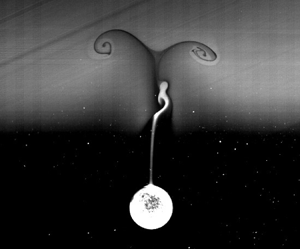
A series of images, corresponding to figure 9, showing the wake development during the entire settling process, are presented in figure 10. The settling process is divided into four stages, as indicated by vertical dashed lines in figure 9(b), and the corresponding wake behaviour is observed in each stage. The four stages are as follows.
(1) Wake attachment (figures 10a–e). As the particle enters the interface, a large amount of upper fluid is dragged by the particle, creating an attached wake. The velocity of the particle decreases rapidly, and the deceleration reaches its maximum at the end of this stage (figure 9b).
(2) Wake detachment (figures 10f–j). At this stage, most of the attached wake detaches from the particle and returns to its neutral position. A long, thin column of lighter fluid remains attached to the centre axis above the particle. As the volume of attached lighter fluid decreases due to the wake detachment, the extra buoyancy diminishes, resulting in a reduced contribution to the stratification drag (refer to the variation of
 $F_{sb}$ in figure 17). Concurrently, the particle's velocity continues to decline, and the acceleration diminishes compared to the first stage (figure 9b). By the end of this stage, the particle loses over $90\,\%$ of its initial entering velocity $U_u$.
(3) Transient bouncing (figures 10k–q). The particle comes to a halt (at
$t=2.61\ {\rm s}$) and rebounds upwards. As the bouncing event approaches, the particle's instantaneous vertical velocity $U(t)$ decreases to near zero, resulting in a small Froude number $Fr(t) = U(t)/ND \ll 1$. This situation could lead to the formation of a thin jet, akin to type A reported by Hanazaki et al. (Reference Hanazaki, Kashimoto and Okamura2009), as depicted in figure 5(k) ($t = 2.4\ {\rm s}$). Furthermore, a strong internal wave emerges at the interface, triggered by the rupture of the wake (figure 11). Nearly all the lighter fluid has detached from the particle by this stage, evidencing a minimal contribution of the extra buoyancy from the dragged light fluid to the drag during the bouncing event. This observation aligns with the force decomposition findings detailed in § 4.3.3.(4) Final sedimentation (figures 10r–t). Following the bouncing and subsequent oscillation, the particle gradually descends to the bottom of the tank. Although it is challenging to discern in figures 10(n–q) before detachment from the particle surface, a small amount of light fluid persists at the particle surface. Note the extended time interval between images. During this phase, the particle settles extremely slowly after traversing the density interface. At
$t=50$ s, its velocity restores to approximately $30\,\%$ of the terminal velocity in the homogeneous lower layer.


A sequence of images showing the bouncing process of a particle settling through a density transition layer, corresponding to figure 9. The two red dashed lines in each image represent the bounds of the interface. The non-dimensional parameters are  $Re_u=347$,
 $Re_l=20$ and
 $Fr=2.5$.

Full image of the internal wave at  $t=8.5$ s between figures 10(o) and 10(p).

These four stages are representative of the typical settling process experienced by a bouncing particle. It is important to note that the actual bouncing process begins only at the third stage, after the wake has detached from the particle. This is consistent with the observations made by Abaid et al. (Reference Abaid, Adalsteinsson, Agyapong and McLaughlin2004) that the particle changes its direction of motion after the rising of the ‘plume’, which in our experiment corresponds to the detached wake. For a monotonically settling particle, the first two stages are identical to those experienced by the bouncing particle, but are followed by a final sedimentation without any bouncing motion.
4.2. Flow structure
To investigate the transient flow structure around the particle, PIV measurement and flow visualisation are conducted simultaneously, using experimental set-up 2 (see figure 1b). In figure 12, we present the results of a particle with  $\rho _p=1126.06\ {\rm kg}\ {\rm m}^{-3}$, bouncing in a stratified fluid with densities
 $\rho _u=1119.37\ {\rm kg}\ {\rm m}^{-3}$ and
 $\rho _l=1125.77\ {\rm kg}\ {\rm m}^{-3}$, and interface thickness
 $L=3.47\ {\rm cm}$. These correspond to non-dimensional parameters
 $Re_u=248$ and
 $Fr=2.49$. As the particle exits the camera's field of view, we estimate
 $Re_l=15$, although this is likely an underestimate due to the limited view size (
 $9.4 \times 7.3\ {\rm cm}^2$) utilised in this experiment.
Illuminated wake (left-hand part of each image) and PIV field (right-hand part) of a particle settling through a density transition layer at  $Re_u=248$,
 $Fr=2.49$ and
 $Re_l=15$. The horizontal red dashed lines mark the bounds of the interface. The arrow at the particle centre indicates the direction of its motion.

Initially, the flow around the particle is similar to that in a homogeneous fluid. However, after the particle enters the interface, accompanying the rupture of the wake, a vortex with direction opposite to that in the homogeneous fluid is formed at the rear of the particle. This vortex grows quickly and detaches from the particle, becoming a vortex ring that remains at the interface (figures 12d,e). As previous research has explained (Zhang et al. Reference Zhang, Mercier and Magnaudet2019; Magnaudet & Mercier Reference Magnaudet and Mercier2020), this vortex is sourced from the baroclinic torque caused by the misalignment between the density and pressure gradients.
Figure 13 presents a close-up view of the vertical velocity distribution around the particle, clearly showing a strong upward flow, referred to as a jet hereafter, formed behind the particle before bouncing occurs (figures 13c–i). The formation of the jet is a transient process. Initially, the jet forms in a U-shaped region (13c) and then develops towards the central axis. It reaches maximum strength at approximately  $1.5D$ above the particle, when the main part of the wake detaches (figure 13d). Subsequently, it transforms into a long, thin jet at the rear of the particle, and a bell-shaped structure (yellow region in figure 13i), similar to type A of Hanazaki et al. (Reference Hanazaki, Kashimoto and Okamura2009), is observed at the end of the jet. It is worth noting that there is a time lag from the formation of the jet to the bouncing of the particle. It is evident in figure 13 that when the maximum jet is formed at 2.4 s, there is a region of downward fluid surrounding the particle. The jet touches the upper particle surface at
 $t=3.6$ s in figure 13(f); until then, it could affect the particle motion directly.
A close-up view of the flow field around the particle, corresponding to figure 12. An upward jet is observed at the centre axis behind the particle just before it changes its direction of motion. The isolines of  $u_z=0$ are depicted as red solid lines, which separate the region with positive and negative vertical velocities. The horizontal red dashed line in (a) indicates the upper boundary of the interface, while in (b–i) it denotes the lower boundary of the interface. The arrow at the particle centre indicates the direction of its motion.

4.3. Force analysis
In this subsection, we analyse the forces acting on a bouncing particle to gain a more in-depth understanding of the bouncing behaviour. The non-monotonic motion of a particle settling in a stratified fluid is known to be caused by the so-called ‘stratification drag’ (denoted  $F_s$). Previous studies have shown that in steady or quasi-steady states,
 $F_s$ is contributed to mainly by two mechanisms: the buoyancy of the dragged upper fluid (
 $F_{sb}$), and the force caused by a specific flow structure (
 $F_{sf}$) (Srdić-Mitrović et al. Reference Srdić-Mitrović, Mohamed and Fernando1999; Higginson et al. Reference Higginson, Dalziel and Linden2003; Yick et al. Reference Yick, Torres, Peacock and Stocker2009; Zhang et al. Reference Zhang, Mercier and Magnaudet2019). Here, we decompose the total force and quantify the contributions of
 $F_{sb}$ and
 $F_{sf}$, using a combined numerical and empirical force decomposition method based on the strategy used by Srdić-Mitrović et al. (Reference Srdić-Mitrović, Mohamed and Fernando1999) and Zhang et al. (Reference Zhang, Mercier and Magnaudet2019).
Our force analysis consists of three steps. First, we describe how we decompose the force. Second, we explain how we calculate the force components. Finally, we present the transient forces acting on a bouncing particle, and analyse the bouncing mechanism.
4.3.1. Force decomposition
To understand the underlying physics of particle bouncing behaviour, we aim to decompose its hydrodynamic force into different components. We begin with the motion equation of a particle settling from rest in a quiescent, homogeneous fluid, which can be written as
 \begin{equation} m_p\,\frac{{\rm d}U}{{\rm d}t}=G+F_b+F_d+F_a+F_h. \end{equation}
The left-hand side represents the total inertia force acting upon the particle, where  $m_p$ is the particle mass. This arises due to the imbalance of forces. On the right-hand side,
 $G$ and
 $F_b$ are respectively the gravity and buoyancy forces of the particle, and the sum
 $G+F_b$ is the reduced gravity of the particle;
 $F_d$ is the steady drag force at the considered time instant,
 $F_a$ is the inertia force of added mass, and
 $F_h$ is the history (Basset) force. Here,
 $F_d$ can be evaluated according to (1.2) and (3.8). In the limit of potential flow,
 $F_a$ can be calculated as
 \begin{equation} F_a={-}\frac{1}{2}\,\rho_f V_p\,\frac{{\rm d} U}{{\rm d} t}. \end{equation}
At the Stokes regime,  $F_h$ has an analytic solution:
 \begin{equation} F_h={-}\frac{3}{2}\,D^2 \sqrt{{\rm \pi} \rho_f \mu} \int _{-\infty} ^t \frac{\dot{U}(\tau)}{\sqrt{t-\tau}}\,{\rm d} \tau. \end{equation}
Although (4.2) and (4.3) do not fit the current parameter range, they demonstrate that the directions of  $F_a$ and
 $F_h$ are opposite to the acceleration. For a decelerating particle, they behave as thrust rather than drag. For a particle settling in a stratified fluid, we follow the same method of drag force decomposition as in (4.1), while introducing an extra term
 $F_s$ to account for the stratification effects. The motion equation becomes
 \begin{equation} m_p\,\frac{{\rm d}U}{{\rm d}t}=G+F_b+F_d+F_a+F_h+F_s. \end{equation}
It is reasonable to further decompose  $F_s$ into two components,
 \begin{equation} F_s=F_{sb}+F_{sj}, \end{equation}
where  $F_{sb}$ represents the enhanced buoyancy caused by dragging the upper fluid to the lower layer, thus modifying the density distributions, while
 $F_{sj}$ is the force caused by the induced flow structure due to the stratification, typically represented by the upward jet flow at the rear of the particle, as observed in figure 13. This upward jet is conjectured to be the dominant flow structure as the particle bounces. Therefore, the equation of motion for a particle settling in a stratified fluid can be written as
 \begin{equation} m_p\,\frac{{\rm d}U}{{\rm d}t}=G+F_b+F_d+F_a+F_h+F_{sb}+F_{sj}. \end{equation}
4.3.2. Force calculation
In this subsubsection, we introduce how we calculate the force components. First, we rearrange (4.6) as
 \begin{equation} m_p\,\frac{{\rm d}U}{{\rm d}t}=G+\underbrace{(F_b+F_{sb})}_{F_{static}}+\underbrace{(F_d+F_a+F_h+F_{sj})}_{F_{dynamic}}. \end{equation}
Here, the total hydro-force  $F_{hydro}$ is split into two parts:
 $F_{static}$ and
 $F_{dynamic}$, where
 $F_{static}$ refers to the hydrostatic force arising from the non-uniform density distribution with zero velocity, whereas
 $F_{dynamic}$ pertains to the force resulting from the non-zero velocity field at a uniform density distribution. Excluding the steady drag
 $F_d$, we note that
 $F_{sf}=F_a+F_h+F_{sj}$ represents the force caused by unsteady flow, i.e. the flow induced by the stratification effect.
In numerical simulation, the velocity, pressure and density fields are obtained by solving (3.1), (3.2), and (3.3). The total hydro-force  $F_{hydro}$ acting on the particle can be calculated using (3.4). The pressure can be divided into two components,
 $p=p_s+p_d$, where
 $p_s$ denotes the hydrostatic pressure caused by the non-uniform density distribution, and
 $p_d$ represents the pressure caused by flow. As the density field is known,
 $p_s$ can be obtained by solving the equation
 \begin{equation} \boldsymbol{\nabla} p_s = \rho \boldsymbol{g}. \end{equation}
Then  $F_{static}$ is calculated as the integration of
 $p_s$ over the particle surface:
 \begin{equation} F_{static}={-}\int _S p_s \boldsymbol{n} \,{\rm d} S, \end{equation}
and  $F_{dynamic}$ is obtained using
 \begin{align} F_{dynamic} &= F_{hydro}-F_{static} \end{align}
 \begin{align} &={-}\int _S p_d \boldsymbol{n} \,{\rm d} S -\int _S \mu ( \boldsymbol{\nabla} \boldsymbol{u}+ \boldsymbol{\nabla} \boldsymbol{u}^{\rm T}) \boldsymbol{\cdot} \boldsymbol{n} \,{\rm d} S. \end{align}
With the density distribution following (2.1), the undisturbed hydrostatic pressure is given by
 \begin{align} p_b &= \int\rho g \,{\rm d}z = \frac{1}{2}\,g(\rho_u+\rho_l)(z-z_{ref}) \nonumber\\ &\quad + \frac{1}{2}\,g(\rho_u-\rho_l)\left[(z-z_{ref})\,{\rm{erf}}(\alpha(z-z_{ref}))+\frac{1}{\alpha \sqrt{\rm \pi}}\exp({-(\alpha(z-z_{ref}))^2})\right]. \end{align}
We can obtain  $F_b$, denoting the buoyancy of the particle in the undisturbed density field, by integrating
 $p_b$ over the particle surface. Then the contribution of
 $F_{sb}$ is quantified using
 \begin{equation} F_{sb} = F_{static}-F_b. \end{equation}
Upon evaluating the steady drag  $F_d$ through (1.2) and (3.8), the drag component arising from unsteady flow can be expressed as
 \begin{equation} F_{sf}=F_{sj} +F_a +F_h=F_{dynamic}-F_d. \end{equation}
Force calculation can also be conducted using the experimental data, with only two steps different from the simulation, as follows.
(1) The hydro-force is calculated using
(4.15)where\begin{equation} F_{hydro}=G-m_p A, \end{equation}$A$ is the acceleration of the particle, obtained by taking the second derivative of the particle position.(2) The density field is reconstructed using the flow visualisation images (left-hand of each image in figure 12), similar to the laser-induced fluorescence method used by Okino et al. (Reference Okino, Akiyama, Takagi and Hanazaki2021). The grey value in these images, representing the concentration of the Rhodamine B dye, is linearly transformed to density. The hydrostatic pressure
$p_s$ is then calculated using these reconstructed density fields. The other steps are the same as those for dealing with the simulation data.


4.3.3. Forces of a bouncing particle
In this subsubsection, we analyse the forces observed in the experiments presented in figure 12, with the reconstructed density fields presented in figure 14. A comparison is made to the simulated results as shown in figure 15. Overall, the evolution of flow structures is consistent between the two methods. The simulation reveals that a small amount of lighter fluid detaches and ascends from the particle surface to the upper layer as bouncing occurs (figures 15h–j). This phenomenon, termed ‘secondary detachment’ and discussed in Wang, Wang & Deng (Reference Wang, Wang and Deng2023), occurs at thin interfaces and high  $Re_u$. Although not captured in the current experiment (figure 14), it was observed in our recent experiments for larger particles with diameters exceeding 2 cm (not presented here).
Reconstructed density field using flow visualisation images from the corresponding experiments shown in figure 12.


Figure 16 compares velocity profiles between the experiment and simulation. Limited by the camera view, the particle has not reached its terminal velocity by the end of the experiment, resulting in  $Re_l=15$ as it exits the view. In contrast, in the simulation, the particle reaches a higher velocity, resulting in
 $Re_l=28$.
Comparison between the simulated and experimental velocity profiles of a particle with density  $\rho _p=1126.06\ {\rm kg}\ {\rm m}^{-3}$ and diameter
 $D=1$ cm, bouncing in stratified fluid with upper and lower densities
 $\rho _u=1119.37\ {\rm kg}\ {\rm m}^3$ and
 $\rho _l=1125.77\ {\rm kg}\ {\rm m}^{-3}$, respectively, over an interface of thickness
 $L=3.47\ {\rm cm}$. The resulting non-dimensional parameters are
 $Re_u=248$ and
 $Fr=2.49$. The lower Reynolds numbers using the end velocities of the experiment and simulation are respectively
 $Re_l=15$ and
 $Re_l=28$.

The decomposed forces are depicted in figure 17, showing simulation (figures 17a,b) and experiment (figures 17c,d) results. The variation of force components shows good agreement. Before entering the transition layer, the particle settles at a constant velocity due to the balance between reduced gravity ( $G+F_b$) and the drag force
 $F_d$. As the particle enters the transition layer, the force components
 $m_p\,{\rm d}U/{\rm d}t$,
 $F_{sb}$ and
 $F_{sf}$ gradually increase from nearly zero values (figures 17a,c). In figure 17(d),
 $F_{sf}$ initially shows a negative value, inconsistent with the simulation (figure 17b). This discrepancy may be attributed to the error in calculating the acceleration during the experiment, as the acceleration magnitude observed in the experiment (see the black line in figure 17d) is slightly larger than in the simulation at the beginning.
Decomposed forces acting on a bouncing particle corresponding to the experiment depicted in figure 12, as well as that from the simulation using the same set of parameters: (a,b) forces computed from numerical simulation data; (c,d) forces derived from experimental data. The shaded areas in (a,c) indicate the interface region, with the black dashed lines denoting the initiation of bouncing behaviour. In (b,d), different stages of the particle's motion are delineated by blue dashed lines: wake attachment (from  $t=0$ to the first blue dashed line), wake detachment (from the first to the second blue dashed lines), transient bouncing (from the second blue dashed line to the end). The final sedimentation stage is not depicted in these plots.

Different stages are separated by vertical blue dashed lines in figures 17(b) and 17(d). The wake buoyancy force  $F_{sb}$ correlates with the volume of attached upper light fluid. It reaches a maximum at the end of the first stage, after the dragging of the wake (see figures 14(b) and 15(b) at
 $t=1.2$ s), just before the wake detaches from the particle. The sudden deceleration of the particle causes the sharp rise in
 $F_{sf}$ due to the inertia, acting as a thrust (positive value) in the first stage. As the particle approaches the third stage,
 $F_{sb}$ decreases as only a thin layer of light fluid remains in the attached wake (see figures 14(f) and 15(f) at
 $t=3.6$ s). Meanwhile,
 $F_{sf}$ becomes the dominant drag force, balancing the reduced gravity (
 $G+F_b$) and preventing further settling of the particle.
When a particle settles through a density interface and  $U_{min}\leqslant 0$ (with the positive direction of the
 $z$-axis pointing downwards), the particle bounces up. At the instant of bouncing (the first time
 $U=0$, indicated by the arrow in figure 16), the particle satisfies the conditions
 \begin{equation} U=0,\quad \frac{{\rm d}U}{{\rm d}t}<0. \end{equation}
Therefore, we have
 \begin{equation} m_p\,\frac{{\rm d}U}{{\rm d}t}= \underbrace{G+F_b}_+{+}\underbrace{F_d}_{0}+\underbrace{F_a}_+{+}\underbrace{F_h}_+{+}\underbrace{F_{sb}}_{-}+\underbrace{F_{sj}}_{-}<0. \end{equation}
The necessary condition for (4.17) to hold is given by
 \begin{equation} |F_{sb}|+|F_{sj}|>|G+F_b|. \end{equation}
Whether the jet is necessary for the occurrence of bouncing depends on the magnitude of  $F_{sb}$. When
 $|F_{sb}|\leqslant |G+F_b|$, the contribution of the jet is necessary for the bouncing behaviour.
In figures 17(b) and 17(d), at the instant of bouncing occurrence (marked by the black dashed line),  $F_{sf}$ plays a dominant role in balancing the reduced gravity. Excluding the positive contribution from (
 $F_a+F_h$),
 $F_{sj}$ becomes the primary component of the drag force. It is important to note that in the current study,
 $F_{sj}$ refers to the force generated by the relative upward flow around the particle, encompassing both pressure and viscosity contributions. This differs from the approach taken by Zhang et al. (Reference Zhang, Mercier and Magnaudet2019), who decomposed the stratification force into three parts: (1) Archimedes drag arising from the entrainment of the lighter fluid, equivalent to
 $F_{sb}$ in our study; (2) inertial force due to the momentum force induced by density disturbances (pressure contribution); and (3) shear force acting on the particle surface induced due to baroclinic vorticity (viscosity contribution). In our scenario, the particle's velocity undergoes rapid fluctuations, leading to swift alterations in the steady drag
 $F_d$. This makes it challenging to accurately quantify the transient effects of pressure and viscosity on
 $F_d$, thus precluding further decomposition of
 $F_{sj}$ into inertia-induced and viscosity-induced stratification forces.
In summary, the mechanism of the bouncing phenomenon is understood as follows. At the early stage,  $F_{sb}$ dominates the drag force due to the large amount of attached light fluid, causing the particle to lose most of its initial velocity. After the particle enters the lower layer, the light fluid detaches and produces an upward jet. Then
 $F_{sb}$ decreases, and the contribution of
 $F_{sj}$ to the drag increases and becomes dominant, causing the particle to continue to decelerate until it bounces up.
4.4. Influence of different parameters
To investigate the impact of various parameters, we conducted three experimental series, each consisting of five tests, as outlined in table 3. By adjusting the densities of the lower ( $\rho _l$) and upper (
 $\rho _u$) fluids, and the thickness of the interface layer (
 $L$), we varied the lower-layer Reynolds number (
 $Re_l$), upper-layer Reynolds number (
 $Re_u$) and Froude number (
 $Fr$). For each test, we released five particles with slightly different properties, as detailed in table 4. The minimum velocity (
 $U_{min}$) attained by each particle during its sedimentation is presented in table 3. A negative
 $U_{min}$ indicates that the particle experienced a bouncing motion. Prior to each test, we accurately measured the density of the particle to within
 $0.01\ {\rm kg}\ {\rm m}^{-3}$, as the density of the particle varies with ambient temperature.
Experimental parameters and minimal velocities.

Particle properties.

Figure 18 displays the non-dimensional minimal velocity ( $U_{min}/U_u$) as a function of
 $Re_l$,
 $Re_u$, and
 $Fr$, using all the experimental data collected. It is evident that
 $U_{min}/U_u$ exhibits a stronger correlation with
 $Re_l$ (
 $1 \leqslant Re_l \leqslant 109$) compared to
 $Re_u$ (
 $152 \leqslant Re_u \leqslant 322$) and
 $Fr$ (
 $2.3 \leqslant Fr \leqslant 5.6$). Notably, bouncing is observed when
 $Re_l$ is less than approximately 30.
The minimal velocity of all the particles in experiments versus lower and upper Reynolds numbers, and Froude number. Here,  $U_{min}/U_u<0$ represents the occurrence of a bouncing motion.

4.4.1. Lower Reynolds number $Re_l$

To investigate the correlation between the minimal velocity and the lower Reynolds number further, we analyse the experimental data from series 1, where the upper Reynolds number and Froude number are  $Re_u=252\pm 16$ and
 $Fr=2.6\pm 0.2$, respectively. In figure 19(a), we plot these experimental results against the lower Reynolds number
 $Re_l$. We also include numerical results at fixed Froude number
 $Fr=2.6$ and upper Reynolds numbers
 $Re_u=258$ and
 $Re_u=349$ for comparison.
The variations of non-dimensional minimum velocity over (a)  $Re_l$ and (b)
 $\Delta \rho _l$. The Froude numbers are
 $Fr=2.6\pm 0.2$ for experiment, and
 $Fr=2.6$ for simulation.

Both the experimental and numerical results demonstrate that  $U_{min}/U_u$ increases linearly with
 $Re_l$. We note that for
 $Re_u\sim 252$, the values of
 $U_{min}/U_u$ in the experiments are uniformly higher than those in the simulations at a similar
 $Re_u\sim 258$. This discrepancy is possibly caused by the incomplete development of
 $U_l$ in the experiments. The velocity measured when the particle exits the viewing window may be smaller than the fully developed
 $U_l$ in the simulations, leading to a smaller
 $Re_l$. To fit the data in figure 19(a), we employ the linear expression
 \begin{equation} \frac{U_{min}}{U_u}=c_1\,Re_{l}+c_2. \end{equation}
Our linear regression analysis yields  $c_1=0.0049$ and
 $c_2=-0.1181$ for the experiments (
 $Re_u=252\pm 16$), and
 $c_1=0.0046$ and
 $c_2=-0.1720$ for the numerical results (
 $Re_u=258$). We identify critical lower Reynolds numbers
 $Re^\ast _l=23.9$ and
 $37.5$ for these two lines, respectively. These critical Reynolds numbers correspond to the position where
 $U_{min}=0$. The values of
 $c_1$ and
 $c_2$ are dependent on
 $Re_u$ and
 $Fr$. In figure 19(a), we observe that a higher upper Reynolds number
 $Re_u=349$ leads to a smaller
 $c_1$ compared to both the experiments and simulations with smaller Reynolds numbers. However, we also note that the critical lower Reynolds numbers
 $Re^\ast _l$ obtained from numerical simulations with different
 $Re_u$ are very similar.
In our study, we adjust the fluid density to achieve various terminal Reynolds numbers, which are not known a priori. These terminal Reynolds numbers are correlated with density ratios through the velocity term, as we introduced at the end of § 1. Prior research has shown that the bouncing behaviour of particles is linked to the fluid density and density ratio (Doostmohammadi & Ardekani Reference Doostmohammadi and Ardekani2014a; Camassa et al. Reference Camassa, Ding, McLaughlin, Overman, Parker and Vaidya2022). Thus it is necessary to investigate the relationship between the minimal velocity and the density ratio. Here, we define the density ratio as  $\Delta \rho _l=(\rho _p-\rho _l)/\rho _l$. Substituting
 $U_l= \nu _l\,Re_l /D$ into (1.3), we can obtain an expression between the density ratio and the Reynolds number:
 \begin{equation} \Delta \rho_l=\frac{3C_{dl} \nu_l ^2\,Re_{l}^2 }{4 g D^3}, \end{equation}
where  $C_{dl}$ is the steady drag coefficient in the lower layer. Combining (4.19) and (4.20), we can obtain the following expression for the dependence of
 $U_{min}/U_u$ on
 $\Delta \rho _l$:
 \begin{equation} \frac{U_{min}}{U_u}=c_1\,\sqrt{\frac{4g D^3}{3 \nu_l ^2 C_{dl}} }\,\Delta \rho_l^{{1/2}}+c_2. \end{equation}
We find that a power-law fitting in the form
 \begin{equation} \frac{U_{min}}{U_u}=c_3\,\Delta \rho_l ^{{1/2}}+c_4 \end{equation}
is suitable for describing the dependence of  $U_{min}/U_u$ on
 $\Delta \rho _l$, as shown in figure 19(b) (recompiled data from figure 19a).
The trajectories and velocity profiles of particle P1 from experiment series 1 are presented in figure 20. Figure 20(a) demonstrates clearly that the bouncing behaviour substantially prolongs sedimentation time. While the particle enters the interface with the same velocity, slight variations in  $Re_l$ significantly affect its behaviour. For relatively large lower-layer Reynolds numbers, such as
 $Re_l=59$, a minimum velocity is observed in figure 20(b), yet the particle continues to descend unidirectionally after passing through the transition layer. We emphasise that all particles have a larger density than the fluid in the tank at all depths. As
 $Re_l$ decreases and crosses a critical value, namely
 $Re_l^\ast$, as we have discussed previously, the particle reverses its direction of motion and ascends for a transient time scale (see figure 20(a) for
 $Re_l=26$ and
 $Re_l=1$). This bouncing phenomenon is characterised by a much deeper and negative minimum velocity, as shown in the depth versus velocity plot in figure 20(b). In this study,
 $Re_l=1$ refers to an extreme case where the particle density (
 $\rho _p=1123.69\ {\rm kg}\ {\rm m}^{-3}$) is near the density of the bottom layer (
 $\rho _l=1123.66\ {\rm kg}\ {\rm m}^{-3}$). In this scenario, the particle experiences an extraordinarily long transient time scale to reach the terminal velocity of the bottom layer. As explained previously by Abaid et al. (Reference Abaid, Adalsteinsson, Agyapong and McLaughlin2004), this long transient is due to the presence of a small boundary layer of upper fluid around the particle, which diffuses exceptionally slowly due to the long diffusion time of salt in water and the absence of strong turbulence diffusion in this low-speed flow state. This is further evidenced by our experimental results in figures 10(p–t), which clearly show that some light fluid remains on the particle surface after the bouncing.
(a) Time trajectories of particles at five different lower Reynolds numbers. The non-monotonic trend indicates a bouncing behaviour. (b) The velocity profiles of particles at five different lower Reynolds numbers. The grey region refers to the density transition layer. Here,  $Fr$ and
 $Re_u$ vary slightly, within
 $Fr=2.4\unicode{x2013}2.5$ and
 $Re_u=236\unicode{x2013}246$.

It is worth noting that previous studies, such as Srdić-Mitrović et al. (Reference Srdić-Mitrović, Mohamed and Fernando1999), did not observe bouncing behaviour. They presented the time trajectories of particles obtained from a series of experiments (see their figure 9), reporting a noticeable decrease in velocity within the transition layer, but without finding reverse motion of the particle. This can possibly be explained by two factors. First, in their experiments, the upper fluid was a mixture of ethyl alcohol and water, which has different diffusion properties compared with our experiment. Thus the lighter upper fluid dragged by the particle could adjust to the surrounding fluid immediately, and weaken the deceleration of the particle. Second, and more importantly, their examined upper Reynolds numbers fall in the range  $0.7\leqslant Re_u\leq 23$, which is much lower than in the current study. As we will discuss later, the upper Reynolds number is also one of the influencing factors for the occurrence of bouncing behaviour. In fact, the second explanation can be related to a deeper physical mechanism, namely the rear buoyant jet, which disappears when
 $Re_u$ is low. As evidenced by the work of Yick et al. (Reference Yick, Torres, Peacock and Stocker2009), there was no sign of such a jet as
 $Re_u\sim 1$.
4.4.2. Froude number $Fr$

We now examine the effects of Froude number. Specifically, we focus on experiment series 3 as presented in table 3. In this experiment, we keep the upper and lower layer fluid densities constant, and vary only the transition layer thickness by releasing particles into the same tank of fluid with a time interval of 24 h. This approach produces transition layer thickness variations in the range  $L=3.15$–13.06 cm, resulting in different Froude numbers.
Figure 21(a) shows the non-dimensional minimum velocities for different particles plotted over the Froude number. Note that the particle density increases from P1 to P5, which causes both the upper and lower Reynolds numbers to increase from P1 to P5. Overall, there is a nearly monotonic increase in the non-dimensional minimal velocity with increasing Froude number, i.e. as the transition layer becomes thicker. Furthermore, there is a noticeable increase in the minimum velocity when the particle density, or equivalently the Reynolds number, increases. However, for heavier particles such as P5, the role of the Froude number in increasing the minimum velocity is less significant (see P5 in figure 21a). In contrast, for lighter particles such as P1 and P2, the influence of the Froude number is considerable. For example, the behaviour of particle P2 changes from bouncing to unidirectional settling as the Froude number increases from  $Fr=2.6$ to
 $Fr=5.1$. It is worth noting that for P2, the lower Reynolds number (
 $Re_l=28$) is very close to the critical Reynolds number
 $Re_l ^ \ast$. We did not observe any bouncing phenomenon for P3, P4 and P5 in figure 21.
(a) The non-dimensional minimum velocity versus Froude number for five particles. The lower and upper Reynolds numbers are: P1,  $Re_l=12$,
 $Re_u=286$; P2,
 $Re_l=28$,
 $Re_u=295$; P3,
 $Re_l=44$,
 $Re_u=303$; P4,
 $Re_l=59$,
 $Re_u=306$; P5,
 $Re_l=77$,
 $Re_u=317$. (b) The velocity profiles of particle P2 versus the vertical position at five Froude numbers. The vertical dashed lines indicate the bounds of the density transition layers.

In figure 21(b), we present the velocity profiles of particle P2 at different Froude numbers. The Froude number significantly alters the evolving profile of particle settling velocity. We observe that the bouncing motion occurs after the particle leaves the transition layer (see  $Fr=2.6$ and 3.7 in figure 21b), while the minimum velocity is reached within the transition layer for those tests without bouncing (see
 $Fr=4.5$, 4.9 and 5.1 in figure 21b). We also observed an interesting phenomenon: the particle restores to a higher settling velocity for the lower Froude number tests than that with high Froude numbers. This behaviour might be caused by the more pronounced diffusion induced by the jet flow. The jet flow can enhance the turbulence diffusion and diffuse the remaining upper layer fluid attached to the particle to its ambient lower layer fluid.
4.4.3. Upper Reynolds number $Re_u$

We now investigate the effects of the upper Reynolds number ( $Re_u$) using numerical simulations. In figure 22(a), we present the non-dimensional minimum velocity versus
 $Re_u$ for five different values of
 $Re_l$ at a fixed Froude number (
 $Fr=2.6$). The trend is clear: the minimal velocity increases as the lower Reynolds number (
 $Re_l$) increases, while at a fixed
 $Re_l$, the minimal velocity decreases with increasing
 $Re_u$, except for
 $Re_l=13$, where all minimal velocities are negative, indicating bouncing for all cases. We examine a special case,
 $Re_l=37$, where the minimum velocity becomes negative as the upper Reynolds number increases to
 $Re_u=292$. In figure 22(b), we plot the variations of settling velocity with depth for this special case. Despite the distinct differences in entering velocities of the particle among different tests, their minimal velocities are considerably similar. Furthermore, they reach minimal velocities at nearly the same depth. From figure 18, we understand that
 $Re_l=37$ is near the critical Reynolds number for bouncing occurrence, making this special case highly sensitive to parameters such as the upper Reynolds number
 $Re_u$. As shown in figure 22(b), the particle moves unidirectionally for
 $Re_u=127$,
 $190$ and
 $244$, while reversing its motion direction for
 $Re_u=292$ and
 $337$.
(a) The non-dimensional minimal velocity versus the upper Reynolds number at five lower Reynolds numbers, with  $Fr=2.6$. (b) The velocity versus vertical position corresponding to
 $Re_l=37$ in (a).

We stress that the upper Reynolds number  $Re_u$ plays a non-negligible role only when the bottom-layer Reynolds number
 $Re_l$ is close to its critical value for bouncing. However, we note that the currently studied upper Reynolds numbers, in both experiments and numerical simulations, are kept at a certain order,
 $Re_u \sim O(100)$. A much lower
 $Re_u$, such as
 ${\sim }O(1)$, would give no sign of bouncing, as discussed in § 4.4.1.
4.4.4. Identification of the bouncing regime in ($Re_u, Fr)$ space

Given that the bouncing behaviour is determined primarily by the lower Reynolds number  $Re_l$, while the other two parameters,
 $Re_u$ and
 $Fr$, can also play a role, as discussed in §§ 4.4.2 and 4.4.3, a better visualisation can be obtained by examining their combined effects. To illustrate, we present two maps in the parametric space of
 $Re_u$ and
 $Fr$ for two selected lower Reynolds numbers,
 $Re_l=13$ and
 $37$, with the contours representing the minimal velocities, in figure 23. It is evident from the figure that the bouncing phenomenon occurs in the higher
 $Re_u$ and lower
 $Fr$ regime, i.e. the upper left regions of the maps. A direct comparison between figures 23(a) and 23(b) indicates that the bouncing regime decreases for higher
 $Re_l$, further demonstrating that
 $Re_l$ is the dominant parameter. When
 $Re_l$ is low, the particles are more likely to bounce after passing through the transition layer.
Maps of non-dimensional minimal velocities of the settling particle at (a)  $Re_l=13$, and (b)
 $Re_l=37$.

By simulating in the same  $(Re_u, Fr)$ parametric space for different values of
 $Re_l$, we summarise the critical lower Reynolds numbers
 $Re^ \ast _{l}$ in table 5. At high
 $Fr$ and low
 $Re_u$, the particle velocity varies smoothly from top to bottom, as shown in figures 21(b) and 22(b). In these cases, we cannot observe bouncing motion for the smallest density difference that we tested (corresponding to
 $Re_l=13$). Therefore, we have not presented
 $Re^ \ast _{l}$ values for these cases. It can be seen from table 5 that
 $Re^ \ast _{l}$ varies from
 $14.4$ to
 $46.2$, depending on different combinations of
 $Re_u$ and
 $Fr$. We should point out that the variations of
 $Re^ \ast _{l}$ with
 $Fr$ at a fixed
 $Re_u$ are not always monotonic, particularly when
 $Re_u$ is high.
Critical lower Reynolds number  $Re_{l}^\ast$ in the
 $(Re_u, Fr)$ space.

4.5. Discussion on the strength of the buoyant jet
To better understand the phenomenon of particle bouncing, it is important to examine the strength of the jet flow induced by the fluid. This can be achieved by quantifying the maximum jet velocity for each combination of  $Re_u$ and
 $Fr$, as shown in figure 24. In this figure, the lower Reynolds number is fixed at
 $Re_l=37$. The maximum magnitude of jet velocity is identified at each test, which is scaled by the lower layer terminal velocity
 $U_l$. This non-dimensional jet velocity
 $u_j/U_l$ is dependent primarily on
 $Re_u$, and its magnitude increases with increasing
 $Re_u$.
Jet velocities with maximum magnitudes in  $(Re_u,Fr)$ space at
 $Re_l=37$. The negative value refers to an upward jet.

The jet velocity also exhibits a small dependency on  $Fr$, decreasing in magnitude as
 $Fr$ decreases. A higher magnitude of the jet leads to a greater drag force, resulting in a smaller
 $U_{min}$ for the particle. The variation in jet strength provides a reasonable explanation for the observed trends in
 $U_{min}$ with respect to changes in
 $Re_u$ and
 $Fr$ (see figures 21(b) and 22(b)), that the decreasing of
 $U_{min}$ with increasing
 $Re_u$ or decreasing
 $Fr$ is due to the increase in the upward jet velocity.
In previous research, Camassa et al. (Reference Camassa, McLaughlin, Moore and Vaidya2008) proposed a critical criterion for bouncing behaviour given by the equation
 \begin{equation} (\rho_p - \rho_l)V_p = (\rho_l - \rho_u)V_d, \end{equation}
where  $V_p$ represents the volume of the particle, and
 $V_d$ represents the volume of the drift, which is the ‘wake’ formed at the rear of the particle as described in § 4.1. The satisfaction of (4.23) is based on three assumptions: (1) the bouncing motion occurs in the lower layer; (2) the unsteady forces
 $F_a$ and
 $F_h$ are negligible; (3) the stratification drag comes entirely from the buoyancy of the drift. These assumptions lead to a linear relationship between the densities of the fluid layers and the particle, as supported by experimental data and potential energy analysis in Camassa et al. (Reference Camassa, Ding, McLaughlin, Overman, Parker and Vaidya2022).
Equation (4.23) yields a linear correlation between the density triplet  $(\rho _u, \rho _l, \rho _p)$ and
 $\Delta \rho _l = (\rho _p - \rho _l)/\rho _l$, given by
 \begin{equation} \Delta \rho_l ={-}\frac{V_d}{V_p}\,\frac{\rho_u}{\rho_l} + \frac{V_d}{V_p}. \end{equation}
Figure 25(a) shows the variation of the critical density ratio  $\Delta \rho _l^ \ast$ over
 $\rho _u/\rho _l$ at
 $Fr=2.6$ and
 $Fr=3.6$, corresponding to the critical cases presented in the first two columns of table 5. A quadratic fit is found to be more appropriate for the data than a linear regression.
(a) The variation of critical density ratio  $\Delta \rho _l ^\ast$ over the density ratio
 $\rho _u/ \rho _l$. (b) The variation of jet velocity over density ratio
 $\rho _u / \rho _l$ at
 $Re_l=13$.

We propose a possible explanation for the quadratic association between  $\Delta \rho _l^\ast$ and
 $\rho _u/\rho _l$. As demonstrated in §§ 4.1 and 4.3.3, the jet dominates the stratification drag as the particle bounces. Assuming that the stratification drag is entirely due to the relative motion of the surrounding fluid with respect to the particle, the force balance can be expressed as
 \begin{equation} (\rho_p-\rho_l)gV_p = \tfrac{1}{2}C_d \rho_l U_r^2 S_p, \end{equation}
where  $U_r$ is the fluid velocity relative to the particle, and
 $C_d$ is the steady drag coefficient. Equation (4.25) leads to a critical criterion for bouncing behaviour, given by
 $U_r \geqslant U_l$. This criterion yields a quadratic relationship between
 $\Delta \rho _l^*/\rho _l$ and
 $U_r$, given by
 \begin{equation} \Delta \rho_l = \frac{3C_d}{2gD}\,U_r^2. \end{equation}
The flow velocity  $U_r$ can be represented by the jet velocity
 $u_j$ when the particle approaches zero velocity. In the studied parameter range, it was found that the jet velocity is linearly related to
 $\rho _u/\rho _l$ when
 $Fr$ is fixed, as shown in figure 25(b).
Based on the findings presented in (4.25), it can be inferred that there exists a quadratic correlation between  $\Delta \rho _l ^ \ast$ and
 $\rho _u / \rho _l$. This observation highlights the significance of the jet velocity in determining the critical regime for the bouncing motion at the current parameter range.
5. Conclusions
In the present study, we conduct a comprehensive investigation into the physical mechanisms behind the bouncing behaviour, or reverse motion, of a spherical particle settling through a three-layer density-stratified fluid. Our research aims to reveal the forces acting on the particle and their correlation with the flow structure. We cover a wide range of parameters, including the lower-layer Reynolds number ( $1\leqslant Re_l\leqslant 125$), upper-layer Reynolds number (
 $115\leqslant Re_u\leqslant 356$), Froude number (
 $2\leqslant Fr\leqslant 7$) and Prandtl number (
 $Pr\approx 700$) for a salinity-stratified fluid.
First, we decompose the forces acting on the particle into different components, and correlate them with the flow structure. We observe four sequential stages of settling, including wake attachment, wake detachment, transient bouncing and final sedimentation. Two mechanisms are identified that contribute to drag enhancement, namely the buoyancy of the attached upper fluid and the force induced by the buoyancy jet flow, which arises from a specific flow structure. During the first two stages, the force component  $F_{sb}$ due to the attached upper fluid in the wake contributes mostly to the drag enhancement. However, at the third stage, most of the upper fluid has detached from the particle, and
 $F_{sb}$ becomes less significant. Instead, the force component
 $F_{sj}$ induced by the jet flow appears to be dominant. We confirm the existence of this jet flow through our experimental measurements, and we conclude that it is a necessary condition for the occurrence of bouncing motion.
Next, we investigate the influence of  $Re_l$,
 $Re_u$ and
 $Fr$. We monitor the minimal settling velocity of the particle, and a negative value indicates a bouncing motion. We find that the lower Reynolds number
 $Re_l$ is the most significant determinant parameter. Our experiments reveal that bouncing motion occurs below a critical lower Reynolds number approximately
 $Re^{\ast }_{l}=30$. In the numerical simulations, the highest value for this critical number is
 $Re^{\ast }_{l}=46.2$, which is limited to the currently studied parametric ranges. Moreover, by quantifying the strength of the jet flow, we find a consistency between the maximum magnitude of jet velocity in the flow fields and the minimal settling velocity for the particle, plotted in the same
 $(Re_u, Fr)$ space. This demonstrates the significance of jet flow on the particle's bouncing motion.
Although our study provides valuable insights into the bouncing behaviour of particles settling through a density-stratified fluid, it is clear that further research is needed. For instance, it would be interesting to consider a cluster of particles, where interactions between particles can lead to more complex and intriguing settling behaviours. Also, particles with irregular shapes can be investigated, which would more closely resemble real-world scenarios, such as the aggregation of marine snow.
Funding
This research has been supported by the National Natural Science Foundation of China (grant no. 92252102). S.W. gratefully acknowledges the hospitality of the Department of Applied Mathematics and Theoretical Physics, University of Cambridge.
Declaration of interests
The authors report no conflict of interest.



