I. INTRODUCTION
Wireless communication systems use radio frequency (RF) signals to transmit data between base stations to mobile users. The RF power amplifier (PA) is located within the base station transmitter and is a key component of the down-link connecting the base station to the mobile.
In the RF transmission of digital information, sampled data sequences are converted from digital to RF and amplified. For a linear system most of the power transmitted by the base station is confined to an allocated bandwidth, which is referred to as a channel. However, PAs operating close to saturation exhibit an undesired nonlinear behavior, generating a distortion spectrum several times wider than the allocated channel. This broadening of the transmitted spectrum is referred to as spectral regrowth and should be compensated.
The interaction of the input signal with the PA nonlinearity generates both harmonic and intermodulation distortion (IMD). In most RF transmitters, a filter is placed after the PA to limit the transmit bandwidth. The pass band spans, typically, several channels: for example, in WCDMA [1] the transmit band may be 60 MHz wide, whereas the individual channels are 5 MHz wide. As a result, the transmit filter can be relied upon to remove the harmonics of the carrier frequency, but not the IMD products of the signal modulation. The latter needs to be compensated using a linearization approach. A popular choice is predistortion applied at the digital baseband.
Digital predistortion (DPD) reduces the transmitted IMD by applying an inverse nonlinearity to the input signal, while it is in its digital baseband representation. The DPD module may use an arbitrarily high number of coefficients to define the inverse nonlinearity. However, to minimize the residual distortion transmitted, it is desirable to estimate and adapt the coefficients based on digital measurements from a receiver observing the PA output. The rank of the coefficient estimation is constrained in part by the bandwidth through which the PA output signal is observed. It is desirable to use an independent measure of the IMD to select the appropriate model order for the coefficient estimation when the observation bandwidth (OBW) is constrained.
The amount of transmitted power appearing outside of the allocated channel is strictly limited by government agencies in order to avoid interference with adjacent channels. Specifications for the various digital modulation formats define maximum allowable levels of spectral regrowth as a function of the frequency offset from the allocated channel. They are often specified as an adjacent channel power (ACP), which is the power integrated over an idle adjacent channel, or as an adjacent channel power ratio (ACPR), which is the ACP divided by the power integrated over the active allocated channel.
It is proposed that a second (less inexpensive) receiver be used to measure the adjacent channel power. To avoid confusion, measurements from the first-mentioned receiver used for coefficient estimation are referred to as “observations” and those from the second-mentioned receiver are referred to as “adjacent channel power”. By measuring the ACP outside of the bandwidth of the observation path, the effect of the estimator's model order on the overall distortion cancellation becomes apparent. Thus, the OBW becomes the constrained resource, and the ACPR becomes the trade-off measure used to select the appropriate model order of the coefficient estimation.
This paper expands upon the work described in [Reference Braithwaite2]. It is written in part because of the recent need to linearize wider bandwidth signals and in response to requests by other researchers for additional information.
II. BACKGROUND
In this paper, the nonlinear behavior of the PA is compensated using DPD. In particular, the challenge of performing adaptive DPD based on an observation pass band that is narrower than the bandwidth of the discernible IMD products is addressed.
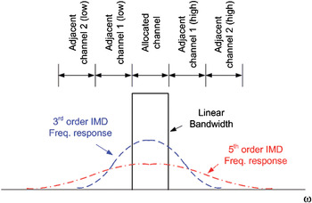
The nonlinearity in the PA can be modeled by a polynomial function of the input signal. Consider the PA response to a Gaussian noise input signal that is band limited to fill the allocated channel. The output spectrum is the sum of the linear component and several intermodulation modes (the third- and fifth-order IMD products are shown in Fig. 1) [Reference Braithwaite and Luo3]. The linear component, also referred to as a carrier signal, remains within the allocated channel whereas the distortion spreads into the adjacent channels. The IMD bandwidth increases with the polynomial order. However, a significant portion of the distortion lies within the allocated channel.
Output spectra for the linear signal, as well as the third- and fifth-order intermodulation distortion products. Also shown are the allocated and adjacent channels. Note the increase in IMD bandwidth with the polynomial order. From [Reference Braithwaite and Luo3].

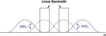
The RF transmitter may transmit several carrier signals occupying nearby channels. In such cases, the IMD comprises components originating from the intermodulation within individual carriers as well as intermodulation between carriers. The effect of the latter is to spread the distortion over a much larger bandwidth, as shown in Fig. 2.
Linear and third-order IMD spectra for a two-carrier signal. Note the increased bandwidth of the distortion spectrum arising from intermodulation between carriers.

The nonlinear behavior of a PA can be classified as memoryless or memory-based. For the former, the nonlinear modes are functions of the instantaneous input only. For the latter, the nonlinear modes are also affected by past input values. The PA memory alters the frequency response of the distortion generated and increases the number of predistortion coefficients needed for wide bandwidth IMD cancellation.
The memory effects exhibited by PAs tend to be more discernible for wide bandwidth input signals, such as those comprising multiple carrier signals. In particular, dramatic memory effects are common with the Doherty amplifier configuration, which is popular in cellular base stations due to its high efficiency when operating at power levels near saturation [Reference Cripps4].
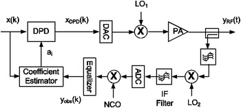
The digitally predistorted transmitter used in this paper is shown in Fig. 3. The digital input and predistorted signals are denoted by x(k) and x DPD(k), respectively. The RF output is
Digital transmitter with predistortion module, estimator, and narrow bandwidth output observation path. Adapted from [Reference Braithwaite2].

 $$y_{RF} \lpar t\rpar =G_{PA} \left[{h\lcub x_{DPD} \lpar k\rpar \rcub \exp\! \lpar j \omega _c t\rpar } \right]\comma \eqno \lpar 1\rpar$$
where G PA is the nonlinear gain of the PA, h{} represents the reconstruction filter used in the digital-to-analog conversion, and ω c is the LO1 frequency. The observation path captures a digital measurement of the output, denoted by y obs(k), by down-converting the RF output to an intermediate frequency (IF) using LO2, bandpass filtering, digitizing, down-converting the digital IF to baseband using a numerically controlled oscillator (NCO), then equalizing for gain flatness.
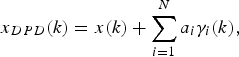
The DPD module generates several nonlinear modes derived from the input signal x(k). That is, the predistorted signal is
 $$x_{DPD} \lpar k\rpar =x\lpar k\rpar +\sum\limits_{i=1}^N {a_i \gamma _i } \lpar k\rpar \comma \eqno\lpar 2\rpar$$
where γi(k) are nonlinear functions of x(k) referred to as basis waveforms, a i are complex coefficients, and N is the order of the DPD model. By weighting the nonlinear basis waveforms correctly, distortion is generated that cancels the IMD generated subsequently by the PA nonlinearity. To accommodate the increased bandwidth of the nonlinear basis waveforms, the sampling rate after the DPD module must be several times the Nyquist rate of the linear signal x(k).
The selection of the basis waveform set is important for the predistortion to achieve the required distortion cancellation. For the memoryless DPD case, the basis waveforms are
 $$\gamma _i \lpar k\rpar =\left\vert {x\lpar k\rpar } \right\vert ^{p - 1} x\lpar k\rpar \comma \eqno \lpar 3\rpar$$
where p is the polynomial order and the index i is a function of p. The DPD model order N tends to be small and is bounded by the highest polynomial order (denoted by P) in the basis set. In some implementations, only the odd polynomial orders are used, thereby reducing the size of N.
For the case of a DPD module with memory correction capability, the DPD model order N exceeds the highest polynomial order P. One possible basis set with memory is the Volterra series, which produces a large number of basis waveforms. The basis waveforms for the polynomial order p = 3 are
 $$\gamma _i \lpar k\rpar =x\lpar k - m_1 \rpar x\lpar k - m_2 \rpar x^{\ast} \lpar k - m_3 \rpar \comma \eqno \lpar 4\rpar$$
where –M ≤ m 1, m 2, m 3 ≤ M and i is a function of p, m 1, m 2, and m 3. The DPD model order is N = (2M + 1)3 for p = 3, which is already large, and becomes exponentially larger as higher values of p are included in the basis set. In addition, many of the basis waveforms in (4) are duplicated. As a result, pruned versions of the Volterra series are used for memory correction in practical implementations [Reference Zhu, Pedro and Cunba5].
A popular memory correction approach implements the predistortion as a nonlinear finite impulse response (FIR) structure with adaptable coefficients. The FIR can be applied to either the gain term [Reference Braithwaite6] or the distortion [Reference Ding7]. For the former case, the basis waveforms are
 $$\gamma _i \lpar k\rpar =\left\vert {x\lpar k - m\rpar } \right\vert ^{p - 1} x\lpar k\rpar \comma \eqno \lpar 5\rpar$$
where –M ≤ m ≤ M and i is a function of p and m. The DPD model order is N = P*(2M + 1) assuming the FIR size, 2M + 1, is the same for each polynomial order, p. The basis set (5) is referred to as a gain polynomial. An alternative basis set, referred to as a memory polynomial, uses
 $$\gamma _i \lpar k\rpar =\left\vert {x\lpar k - m\rpar } \right\vert ^{p - 1} x\lpar k - m\rpar \comma \eqno \lpar 6\rpar$$
as the basis waveforms.
The DPD coefficients are tuned adaptively to provide effective distortion compensation. This requires an observation of the signal present at the output of the PA. The RF observation signal is converted to the digital baseband using a receiver and compared to the original input signal x(k). Differences between the input signal x(k) and the output signal y(k) are used to estimate the coefficient adjustments required to improve the predistortion. Note that at this point, output signal y(k) and the observed signal y obs(k) are considered to be the same signal. However, they are treated as different signals in Section III, where y obs(k) is a band limited version of y(k).
The coefficients are adjusted to minimize the residual distortion in the output signal, which is measured using time-aligned samples of the input and output signals: x = [x(1)···x(K)]T and y = [y(1) ···y(K)]T, respectively, where K is the buffer size. Let the error signal and basis set be denoted by
 $$\varepsilon \lpar k\rpar =G_o ^{ - 1} y\lpar k\rpar - x\lpar k\rpar \comma \eqno \lpar 7\rpar$$
 $$\psi \lpar k\rpar =\lsqb \matrix{\! {\gamma _1 \lpar k\rpar } & \cdots & {\gamma _N \lpar k\rpar } \cr } \rsqb \comma \eqno \lpar 8\rpar$$
respectively, where G o is the nominal gain. The nominal gain used in this paper is
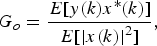 $$G_o=\displaystyle{{E\lsqb y\lpar k\rpar x^{\ast} \lpar k\rpar \rsqb } \over {E\lsqb \left\vert {x\lpar k\rpar } \right\vert ^2 \rsqb }}\comma \eqno \lpar 9\rpar$$
where E[ ] denotes the expected value. The estimate of the coefficient offset is
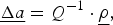 $$\underline {\Delta a}=Q^{ - 1} \cdot \underline \rho\comma \eqno \lpar 10\rpar$$
where Δa = [Δa 1,…, Δa N]T are the coefficient offsets,
 $$Q=E\lsqb \psi ^H \lpar k\rpar \psi \lpar k\rpar \rsqb =\displaystyle{1 \over K}\sum\limits_{k=1}^K {\psi ^H \lpar k\rpar \psi \lpar k\rpar }\comma \eqno \lpar 11\rpar$$
 $$\underline \rho=E\lsqb \psi ^H \lpar k\rpar \varepsilon \lpar k\rpar \rsqb =\displaystyle{1 \over K}\sum\limits_{k=1}^K {\psi ^H \lpar k\rpar \varepsilon \lpar k\rpar }\comma \eqno \lpar 12\rpar$$
and ()H denotes conjugate transpose. The updated coefficients are
 $$\underline a \lpar t_{l+1} \rpar =\underline a \lpar t_l \rpar - \eta \underline {\Delta a}\comma \eqno \lpar 13\rpar$$
where a = [a 1,…, a N]T, t l indicates the iteration number, and η < 1. The process of capturing data, estimating coefficient offsets, and updating the coefficients is repeated, further reducing the output distortion.
The estimation can also be done in the frequency domain. Let the Fourier transforms of x(k), y(k), γi(k), ψ(k), and ɛ(k) be denoted by X(ω k), Y(ω k), Γi(ω k), Ψ(ω k), and E(ω k), respectively, where
 $$\Psi \lpar \omega _k \rpar =\lsqb \matrix{ {\Gamma _1 \lpar \omega _k \rpar } & \cdots & {\Gamma _N \lpar \omega _k \rpar } \cr } \rsqb \eqno \lpar 14\rpar$$
and
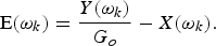 $${\rm E}\lpar \omega _k \rpar =\displaystyle{{Y\lpar \omega _k \rpar } \over {G_o }} - X\lpar \omega _k \rpar . \eqno \lpar 15\rpar$$
We have
 $$Q=E\lsqb \Psi ^H \lpar \omega _k \rpar \Psi \lpar \omega _k \rpar \rsqb =\displaystyle{1 \over K}\sum\limits_{k=1}^K {\Psi ^H \lpar \omega _k \rpar \Psi \lpar \omega _k \rpar } \eqno \lpar 16\rpar$$
and
 $$\underline \rho=E\lsqb \Psi ^H \lpar \omega _k \rpar \!\cdot \!{\rm E}\lpar \omega _k \rpar \rsqb =\displaystyle{1 \over K}\cdot \!\sum\limits_{k=1}^K {\Psi ^H \lpar \omega _k \rpar\! \cdot\! {\rm E}\lpar \omega _k \rpar } . \eqno \lpar 17\rpar$$
The Fourier-based estimation is used in the proposed approach described in Section III.
Careful selection of the basis set ψ(k) minimizes the number of basis waveforms γi(k) used, ensuring that the matrix Q is well conditioned. However, the selection criteria for the basis set that satisfies the DPD module's requirement for IMD reduction competes with the estimator's requirement for a well-conditioned matrix Q. A large basis set that describes accurately the physical properties of the PA provides good IMD cancellation, but only if the coefficients are selected correctly. Unfortunately, the input signal x(k) often lacks the statistical content in terms of amplitude variation and spectrum to excite fully the space spanned by the basis set ψ(k). This causes the matrix Q to be rank deficient. Thus, the appropriate model order for the coefficient estimation depends on the input signal statistics as much as the PA nonlinearity.
It is possible to reduce the model order of the estimation compared to the DPD model order. The former will be denoted by N est and the latter by N. The difference in the model orders of the DPD module and the coefficient estimator can be resolved by using an eigenvalue decomposition of the matrix Q, as shown in the next section. When the input signal x(k) is not rich enough to provide a full rank matrix Q, the number of independent coefficient adjustments for a given iteration of (10) is reduced to equal the number of dominant (or discernible) eigenvalues available in Q. This technique is referred as singular value decomposition (SVD).
The above-mentioned estimation assumes that the bandwidth of the output observation path is larger than the bandwidth of the widest basis waveform. This is not always the case when the input signal x(k) has a wide bandwidth and the maximum polynomial order of the basis set ψ(k) is high.
The implementation of the observation receiver shown in Fig. 3 uses IF sampling, which has advantages in terms of cost, as well as avoiding offsets and imbalances associated with a demodulator used in zero-IF down-conversions. However, the OBW is reduced by at least a factor of two compared to a zero-IF receiver. Assume the analog-to-digital converter (ADC) and the digital-to-analog converters (DAC) within Fig. 3 have the same sampling rate, but that the transmit path uses a zero-IF up conversion (dual DACs). The observation path shown in Fig. 3 does not have enough bandwidth to measure the entire frequency content of the widest basis waveforms that can be generated by the DPD module.
It is not necessary to measure the full spectrum of the IMD waveform to adapt the DPD coefficients. Zhu [Reference Zhu8] has shown that the output of a nonlinear function in response to a band limited input signal need only be sampled at the Nyquist rate of the input signal x(k) rather than the wider bandwidth of the DPD signal x DPD(k) if the nonlinear function is a one-to-one continuous mapping. With respect to the present application, this means that the OBW must be as wide as the linear signal bandwidth to estimate the coefficients if the DPD module is memoryless.
In general, the coefficient estimate based on (10) will have poor IMD cancellation over a wide bandwidth because the IF filter in the observation path will be interpreted incorrectly as PA memory. In such a case, any memory correction available within the DPD module will degrade the distortion cancellation compared to a memoryless model in the portion of the spectrum outside of the OBW. Thus, there is a penalty associated with over-specifying the model order of the estimation N est when the observation path is not perfect.
It is shown in Section III that deleterious effects of the limited OBW are minimized by filtering the basis waveforms ψ(k) within the estimator so that the comparison between the observed PA output y obs(k) and the basis waveforms is made over the identical frequency band. The filtering alters the frequency weighting of the coefficient estimate and is applied only to the estimator. The basis waveform set used by the DPD module is not altered, making it possible to extrapolate the distortion cancellation beyond the observed bandwidth (OBW). However, there is no guarantee that the unseen IMD will be reduced by the narrow bandwidth optimization. The model order of the estimation N est affects the overall distortion cancellation performance, as shown in Section IV. The selected estimation model order N est should improve distortion cancellation within the OBW without over-fitting so that the IMD products outside of the OBW are at least as low as those achievable using memoryless DPD.
For a DPD module with memory compensation, it is necessary to either expand the OBW or to constrain the model order of the estimator N est so that distortion cancellation occurs outside of the OBW. ACPR provides an independent measure of the residual distortion that is used in Section IV to judge whether the selected estimation model order N est provides adequate cancellation.
III. PROPOSED APPROACH
In this section, the estimation approach is altered so that bandwidth limitations within the observation path do not restrict the predistortion capabilities. When the output signal is measured using a small bandwidth, it is recommended that center frequency of the observation path be adjusted over time using the LO2. Frequency-shifting the observation band allows as much distortion spectral content as possible to be measured. The estimator combines measurements from the different observation bands to improve distortion cancellation over a wider bandwidth. In addition, the model order of the estimation N est is adjusted to obtain a low ACPR outside of the OBWs tested.
The cost function minimized by (10) is
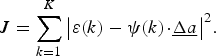 $$J=\sum\limits_{k=1}^K {\left\vert {\varepsilon \lpar k\rpar - \psi \lpar k\rpar \!\cdot\! \underline {\Delta a} } \right\vert ^2 } . \eqno \lpar18\rpar$$
In general, (10) cannot be used to estimate the coefficient offsets Δa for the system shown in Fig. 3 because the observed output y obs(k) is band-limited. That is, y obs(k) is available, but not y(k).
The relationship between the desired output y(k) and the observed output y obs(k) is
 $$L_{IF} \left\{{y\lpar k\rpar } \right\}=y_{obs} \lpar k\rpar \comma \eqno \lpar 19\rpar$$
where L IF{} is the frequency response of the IF filter. In most implementations, y obs(k) would be equalized to obtain the best estimate of y(k). However, equalization can only flatten the pass band of the observation path; it will not restore the part of the spectrum for y(k) lost to band limiting.
An alternative approach is to spectrally weight the estimation (18). That is, superposition is applied to (18), creating a new cost function based on filtered signals:
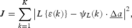 $$J=\sum\limits_{k=1}^K {\left\vert {L\left\{{\varepsilon \lpar k\rpar } \right\}- \psi _L \lpar k\rpar \cdot \underline {\Delta a} } \right\vert ^2 }\comma \eqno \lpar 20\rpar$$
where L{ } is a filter operation and
 $$L\lcub \varepsilon \lpar k\rpar \rcub =G_o ^{ - 1} \cdot L\lcub y\lpar k\rpar \rcub - L\lcub x\lpar k\rpar \rcub \comma \eqno \lpar 21\rpar$$
 $$\psi _L \lpar k\rpar =\lsqb \matrix{ {L\lcub \gamma _1 \lpar k\rpar \rcub } & \cdots & {L\lcub \gamma _N \lpar k\rpar \rcub } \cr } \rsqb .\eqno \lpar 22\rpar$$
The estimate of the coefficient offsets using the band limited signals is
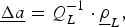 $$\underline {\Delta a}=Q_L ^{ - 1} \cdot \underline \rho _L\comma \eqno \lpar 23\rpar$$
where
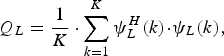 $$Q_L=\displaystyle{1 \over K}\cdot \sum\limits_{k=1}^K {\psi _L ^H \lpar k\rpar \!\cdot\! \psi _L \lpar k\rpar }\comma \eqno \lpar 24\rpar$$
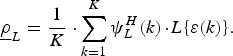 $$\underline \rho _L=\displaystyle{1 \over K}\cdot \sum\limits_{k=1}^K {\psi _L ^H \lpar k\rpar \!\cdot\! L\lcub \varepsilon \lpar k\rpar } \rcub . \eqno \lpar 25\rpar$$
The key requirement in (20) is that the same linear operation L{} must be applied to each of x(k), y(k), and γi(k). We can replace y(k) with y obs(k) as long as we account for the frequency response of the IF filter L IF{} within (21). For example, in the simplest case when L{} is the same as L IF{}, the filtered error signal becomes
 $$L_{IF} \lcub \varepsilon \lpar k\rpar \rcub =G_o ^{ - 1} \cdot y_{obs} \lpar k\rpar - L_{IF} \lcub x\lpar k\rpar \rcub . \eqno \lpar26\rpar$$
However, it is often beneficial to choose a filter response L{} that limits the OBW further. That is, if the bandwidth of L{} is smaller than the OBW of L IF{}, so that L{y(k)} = L{y obs(k)}, then we do not need to know the exact frequency response of the IF filter (assuming the IF filter response is flat within the frequencies of interest).
It is also beneficial to select L{} to notch the input signal x(k), so that L{x(k)} = 0. This has the effect of optimizing the coefficient estimation for the cancellation of out-of-band IMD products, which contribute to the ACPR. In particular, it removes biases in the estimate of Δa that are due to unmodeled in-band errors, which are often larger in power than the distortion generated. The benefits of notching the input signal x(k) are shown in [Reference Braithwaite9].
The digital filter L{} is implemented in the Fourier domain. The frequency response of the estimation filter L(ω k) is the product of a notch filter L notch(ω k) and a band pass filter L OBW(ω k). The frequency response of the notched filter is
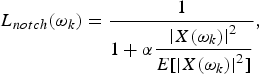 $$L_{notch} \lpar \omega _k \rpar =\displaystyle{1 \over {1+\alpha \displaystyle{{\left\vert {X\lpar \omega _k \rpar } \right\vert ^2 } \over {E\lsqb \left\vert {X\lpar \omega _k \rpar } \right\vert ^2 \rsqb }}}}\comma \eqno \lpar 27\rpar$$
where X(ω k) is the Fourier transform of x(k) and α is a constant controlling the depth of the notch. The frequency response of the band pass filter used to band limit γi(k) and ɛ(k) to fit within the OBW is
 $$L_{OBW} \lpar \omega _k \rpar =\left\{{\matrix{ 1 & {{\rm for}} & {\left\vert {\omega _k - \omega _c } \right\vert \lt \displaystyle{{\omega _o } \over 2}\comma \; } \cr 0 & {} & {{\rm otherwise\comma \; }} \cr } } \right. \eqno \lpar 28\rpar$$
where ω o is the bandwidth of the filter and ω c is the center frequency of the band.
The Fourier-based coefficient estimation is described below. Time-aligned samples of the input signal x = [x(1),…, x(K)]T, observed signal yobs = [y obs(1),…, y obs(K)]T, and basis waveforms γi = [γi(1),…, γi(K)]T are multiplied by Hann windows, then transformed into the Fourier domain using fast Fourier transforms (FFTs) to obtain X(ω k), Y obs(ω k), and Γi(ω k). The filtered values of the basis set and error signal are
 $$\Psi _L \lpar \omega _k \rpar =\lsqb \matrix{ {L\lpar \omega _k \rpar \Gamma _1 \lpar \omega _k \rpar } & \cdots & {L\lpar \omega _k \rpar \Gamma _1 \lpar \omega _k \rpar } \cr } \rsqb \comma \eqno \lpar 29\rpar$$
 $${\rm E}_L \lpar \omega _k \rpar =G_o ^{ - 1} \cdot L\lpar \omega _k \rpar \!\cdot \!Y_{obs} \lpar \omega _k \rpar - L\lpar \omega _k \rpar \!\cdot \!X\lpar \omega _k \rpar \comma \eqno \lpar 30\rpar$$
where
 $$L\lpar \omega _k \rpar =L_{OBW} \lpar \omega _k \rpar \cdot L_{notch} \lpar \omega _k \rpar . \eqno \lpar 31\rpar$$
It is assumed that L(ω k) is band limited enough that L(ω k) Y obs(ω k) = L(ωk) Y(ω k). If not, one must multiply L(ω k) Γi(ω k) and L(ω k) X(ω k) by L IF(ω k) to compensate. The Fourier-based estimates of matrix Q L and vector ρ L become
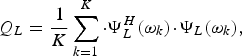 $$Q_L=\displaystyle{1 \over K}\sum\limits_{k=1}^K {\cdot \Psi _L ^H \lpar \omega _k \rpar \!\cdot\! \Psi _L \lpar \omega _k \rpar }\comma \eqno \lpar 32\rpar$$
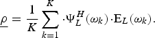 $$\underline \rho=\displaystyle{1 \over K}\sum\limits_{k=1}^K {\cdot \Psi _L ^H \lpar \omega _k \rpar \!\cdot\! {\rm E}_L \lpar \omega _k \rpar }. \eqno \lpar 33\rpar$$
The length of the batches of x, yobs, and γi should be short to reduce the complexity of the FFT computations, preferably K = 2048 samples. In general, at least 16 000 samples are needed for good steady-state results [Reference Zhu, Pedro and Cunba5]. The integration of several 2048 blocks to obtain Δa is performed as follows:
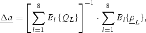 $$\underline {\Delta a}=\left[{\sum\limits_{l=1}^8 {B_l \left\{{Q_L } \right\}} } \right]^{ - 1} \cdot \sum\limits_{l=1}^8 {B_l \lcub \underline \rho _L \rcub }\comma \eqno \lpar 34\rpar$$
where B l{} indicates samples from block l. An advantage of (34) is that the blocks from different filters L{} may be integrated to extend the effective bandwidth of the observation path.
OBW extension is achieved using three LO2 settings to provide spectral measurements above, below, and surrounding the allocated channels containing the input signal x(k). Changing the frequency of LO2 has the effect of moving the center frequency of the observation band. Combining measurements from the three observation bands using (34) provides an improved estimate of the coefficient offset Δa. Note that it is necessary for every observation band to maintain partial overlap with the input spectrum to provide a reference for time-alignment of the input and output signals.
The estimation of Δa using (23) or (34) can be ill-conditioned because Q L often has an insufficient rank. This occurs for two reasons: the signal x(k) does not stimulate all the nonlinear modes spanned by the selected basis set ψ(k) or the OBW is not measuring the modes. The narrow OBW problem is made less severe by using (34) to combine data obtained from different observation bands. The under-stimulated modes problem is due to poor selection of the basis waveform set for the input signal x(k).
The basis set ψ(k) is selected, typically, for the worst-case input signal x(k). For other input signals having less bandwidth or lower magnitude, the basis set ψ(k) will be over-specified. Singular value decomposition (SVD) is used to improve the conditioning of the estimation and avoid the need to change the basis set as a function of the input signal x(k). In such cases, Q L−1 is replaced in (23) by a pseudo-inverse S whose rank is lower.
Assume the eigenvectors of Q L are denoted by vj, where the index j is listed from the largest to smallest eigenvalue λ j. SVD reduces the rank of S from N to N est:
 $$S=V\!\cdot\! D\!\cdot\! V^H \approx Q_L ^{ - 1}\comma \eqno \lpar 35\rpar$$
where V = [v1,…, v N] and D = diag{λ1−1 … λNest−1 0 … 0}. Since the degrees of freedom in the estimation are reduced, condition problems are avoided. Note that the basis set ψ(k) used in the DPD module remains unchanged.
The accuracy of the coefficient estimation is affected by the bandwidth of the observation path (OBW) and the model order of the estimator (N est). In Section IV, various combinations of OBW and N est are tested and compared. It is shown that the estimation model order N est should be reduced when OBW is small to prevent spectral growth outside of the OBW. That is, the excess degrees of freedom in the estimator model should be constrained using SVD (or other regularization method) to avoid coefficient biases and unwanted spectral growth.
IV. RESULTS
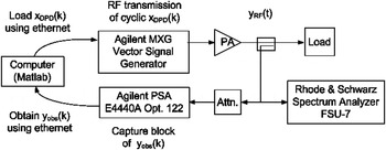
The relationship between the model order of the estimation N est, the OBW, and the ACPR performance is demonstrated experimentally. The test setup shown in Fig. 4 uses an Agilent MXG (arbitrary waveform generator) to generate the RF signal, a high efficiency Doherty PA to amplify it, and an Agilent PSA E4440A (opt. 122) as a receiver to measure y obs(k). A computer running Matlab computes the DPD signal x DPD(k) and loads it into the MXG. It also estimates the DPD coefficients a using the observed output signal y obs(k) extracted from the PSA. The sampling rates of x(k), x DPD(k), and y obs(k) are 100 MHz. A Rhode & Schwarz FSU-7 is used to analyze the output spectrum and measure the ACPR independently. The Ethernet connections between the Matlab code and the MXG/PSA use functions available from the Agilent Download Assistant.
Test bench. Adapted from [Reference Braithwaite2].

The DPD module is implemented using a gain polynomial, defined by (2) and (5). The polynomial orders used are p = [2, 3, 4, 5] and the memory depths (−M ≤ m ≤ M) are M = 12 for p = [2, 3] and M = 6 for p = [4, 5]. This results in a basis set comprising N = 76 waveforms, which is large (intentionally). The coefficient estimation based on (34) is ill conditioned for the input signal used (described below). SVD in (35) is used to reduce the model order of the estimation to one of the following: N est = 5, 10, or 15.
The input signal x(k) comprises two 5 MHz channels of noise separated by 15 MHz. The center frequency is 1960 MHz. Discernible components of the IMD appear at 15 and 30 MHz offsets from the two input signal channels.
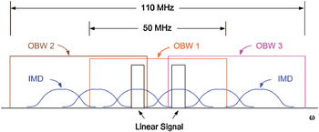
The OBW used by the estimator is limited to 50 MHz using (28). As a result, part of the IMD spectrum is outside of the OBW. To extend the measured bandwidth, the observation pass band is shifted by –30 MHz, 0, and 30 MHz from the center frequency of the input signal. Combining three frequency-shifted pass bands using (34) extends the effective OBW to 110 MHz, as shown in Fig. 5.
Input signal and three observation bandwidths (OBWs). The input signal comprises two 5 MHz noise bands separated by 15 MHz. The OBWs are 50 MHz wide and are offset from the input signal by –30 MHz, 0, and 30 MHz. The effective bandwidth of the three observation paths spans 110 MHz. Adapted from [Reference Braithwaite2].

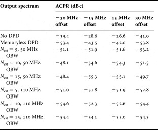
The ACPR for offsets of 15 MHz and 30 MHz from the nearest active channel are denoted by ACPR15MHz and ACPR30MHz, respectively. They are listed in Table 1 for the following cases: no linearization, memoryless DPD only, and memory correction using estimation model orders of N est = [5, 10, 15]. The memoryless DPD case is provided as a baseline. It reduces ACPR15MHz and ACPR30MHz by −14.9 dB and −12.0 dB, respectively, compared to the no linearization case.
ACPR for memory-based DPD using different estimation model orders (N est) and observation bandwidths (OBW).

Let us consider DPD with memory correction for the 50 MHz OBW case. ACPR15MHz falls within the OBW; however, ACPR30MHz is outside of the OBW. Memory correction improves the ACPR for the 15 MHz offset compared to the memoryless DPD: that is, ΔACPR15MHz = [−9.6, −12.6, −13.1] dB for N est = [5, 10, 15], respectively. In contrast, adding memory correction degrades the 30 MHz offset ACPR: ΔACPR30MHz = [+2.3, +5.3, +5.0] dB for N est = [5, 10, 15]. Thus, increasing the estimation model order N est improves IMD cancellation within the OBW and tends to degrades it outside of the OBW.
Now consider the case of DPD with memory correction for an OBW of 110 MHz, which spans both ACPR15MHz and ACPR30MHz. Memory correction improves the ACPR at the 15 MHz offset compared to the memoryless DPD: ΔACPR15MHz = [−9.8, −10.3, −12.1] dB for N est = [5, 10, 15]. Adding memory correction improves ACPR30MHz for the higher two estimation model orders: ΔACPR30MHz = [+2.4, −1.0, −1.0] dB for N est = [5, 10, 15]. Thus, increasing the estimation model order from Nest = 5 to 15 improves distortion cancellation when OBW = 110 MHz.
Assume that the goal of wide bandwidth IMD cancellation is to minimize the worst ACPR among the 15 MHz and 30 MHz offsets. The worst ACPR for the memoryless DPD is −42.0 dB. For the 50 MHz OBW with memory correction, the worst ACPRs are [–51.1, −48.1, –48.4] dB for N est = [5, 10, 15]. The IMD cancellation is best for memory-based DPD with N est = 5 when the OBW is narrow (50 MHz). For the 110 MHz OBW with memory correction, the worst ACPRs are [–51.0, −52.3,–54.1] dB for N est = [5, 10, 15]. An estimation model order of N est = 15 provides the best IMD cancellation when the OBW is wider (110 MHz).
It is interesting to note the effect of additional OBW on the worst ACPR, for a given N est. The ACPR measurements for 50 MHz and 110 MHz OBWs are almost identical for N est = 5, whereas there is a large difference in ACPR30MHz for N est = [10, 15]. In summary, the 50 MHz OBW should use N est = 5 to obtain ACPR < −51 dB and the 110 MHz OBW should use N est = 15 to obtain ACPR < –54 dB.
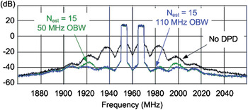
The predistorted output spectra for N est = 15 using 50 MHz and 110 MHz OBWs are shown in Fig. 6. Note the degraded performance of the former at an offset of 30 MHz. From Table 1, it can be seen that using the 50 MHz observation pass band results in a slightly better ACPR15MHz than the wider 110 MHz OBW (up to 1.2 dB); however, ACPR30MHz degrades by 6 dB. This is not a good trade-off because the worst ACPR is increased. Thus, when estimating the DPD coefficients it is preferable to use the widest OBW available and select an estimation model order N est that produces the best ACPR performance.
Output spectra of a Doherty PA for memory-based DPD whose estimation model order is N est = 15 for 50 MHz (green) and 110 MHz (blue) observation bandwidths (OBWs). The uncorrected PA output is also shown (black). See Table 1 for ACPR values. Adapted from [Reference Braithwaite2]. © 2008 IEEE. Reprinted, with permission, from [Reference Braithwaite2].

V. FUTURE RESEARCH
The reduction of the model order of the estimation using SVD (see (35)) is done because the observation measurement (ρL) does not see the nonlinear modes associated with the smaller eigenvectors, [vNest,…, vN]. However, these discarded modes affect the ACPR measurements outside of the OBW. Once the reduced order coefficient set has converged, it is possible to search the sub-space of coefficients spanned by the discarded eigenvectors [v Nest,…, v N] for the minimum ACPR.
The coefficient offset vector, Δa, can be written as a weighted sum of eigenvectors of Q L: that is,
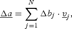 $$\underline {\Delta a}=\sum\limits_{j=1}^N {\Delta b_j \cdot \underline {v} _j }\comma \eqno \lpar 36\rpar$$
where Δb j are complex weights. Similarly, the vector ρL becomes
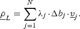 $$\underline \rho _L=\sum\limits_{j=1}^N {\lambda _j\! \cdot\! \Delta } b_j\! \cdot\! \underline v _j . \eqno \lpar 37\rpar$$
Since SVD approximates (37) by using only the dominant eigenvectors, its application reduces the upper bound of the summation from N to N est. The approximation error is modest as long as the ignored eigenvalues, [λNest, …, λN], are small. That is, the narrow OBW estimator cannot see the nonlinear modes associated with the discarded eigenvectors [vNest,…, vN].
The steady-state DPD coefficients become
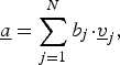 $$\underline a=\sum\limits_{j=1}^N {b_j \!\cdot\! \underline v _j }\comma \eqno \lpar 38\rpar$$
where b j are complex weights. SVD ensures that [b Nest … b N] = [0 … 0]. However, these discarded modes can be adjusted to reduce the ACPR outside of the OBW.
A descent-based search for the minimum ACPR from the sub-space spanned by discarded eigenvectors [vNest … vN] begins with the selection of an orientation, Δθ = [0 … 0 Δb Nest … Δb N]. The orientation Δθ is chosen such that the nonlinear mode δ(k) = ψ(k)*Δθ has energy in the ACPR channels being measured. The coefficient vector b is stepped along this orientation,
 $$\underline b \lpar t_1 \rpar =\underline b \lpar t_0 \rpar - \beta \!\cdot \!\underline {\Delta \theta }\comma \eqno \lpar 39\rpar$$
where β is a step size. Measurements made before and after the step are used to determine the direction (positive or negative) along Δθ that reduces the ACPR. Additional orientations are tested to extract (partial) gradient information, after which a standard line search is performed in the direction having the steepest descent. This process is repeated until no improvement in the ACPR is found. Alternative descent approaches are discussed in [Reference Luenberger10].
VI. CONCLUSION
Wide bandwidth DPD using a narrowband observation path is made possible by using a reduced model order for the estimation and/or by increasing the effective bandwidth of the observation path. The latter is achieved by performing the estimation on several frequency-shifted observation pass bands. The ACPR provides an independent measurement of the distortion cancellation performance that may be used for the optimal selection of the model order of the estimation.
 R. Neil Braithwaite received the B.Sc. degree in electrical engineering from the University of Calgary, Canada, in 1985, and the M.Sc. and Ph.D. degrees from the University of British Columbia, Canada, in 1989 and 1992, respectively. From 1992 to 1995, he conducted postdoctoral work at the University of California, Riverside. He has worked for Computing Devices Company (acquired by General Dynamics) in Ottawa, Canada, from 1985 to 1987, and Nortel in Calgary, Canada, from 1995 to 1997. From 1997 to 2002, he worked for Agilent Laboratories in Palo Alto, CA. He is currently working for Powerwave Technologies in Santa Ana, CA in the Research and Development group. His research interests include signal processing, linearization of RF power amplifiers, and echo cancellation in RF repeaters.