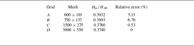
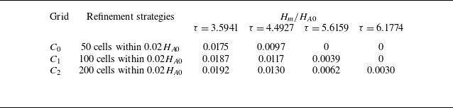
1. Introduction
Shock reflection is a common physical phenomenon in compressible flow which exerts a marked influence on the aerodynamic and aerothermal performance of supersonic vehicles both in internal (Azevedo & Liu Reference Azevedo and Liu1993; Goonko et al. Reference Goonko, Latypov, Mazhul, Kharitonov, Yaroslavtsev and Rostand2003; Arun Kumar & Rajesh Reference Arun Kumar and Rajesh2017) and external flows (Deschambault & Glass Reference Deschambault and Glass1983; Anderson Reference Anderson1989; Surujhlal & Skews Reference Surujhlal and Skews2019). Two canonical configurations exist in steady shock reflection, regular reflection (RR) and Mach reflection (MR), as illustrated in figure 1(a). In early 1940s, von Neumann (Reference von Neumann1945) made use of the inviscid conservation equations across an oblique shock and established two-shock theory and three-shock theory for analytically describing RR and MR, respectively.
von Neumann (Reference von Neumann1943) also proposed two critical conditions, the detachment condition (
 $\theta ^{D}$
) and von Neumann condition (
 $\theta ^{N}$
), which divide incoming Mach number
 $M_{0}$
and wedge angle
 $\theta _{w}$
phase plane into three domains in figure 1(b). Below von Neumann condition is RR domain (RRD) where only RR occurs. Above detachment condition is MR domain (MRD) where only MR occurs. Between these two critical conditions is dual-solution domain (DSD) where both RR and MR are possible. Hornung et al. (Reference Hornung, Oertel and Sandeman1979) first presented hysteresis phenomenon in DSD, they predicted that transition from RR to MR will occur for the detachment condition when increasing
 $\theta _{w}$
. While transition from MR to RR will occur for the von Neumann condition when decreasing
 $\theta _{w}$
. Subsequent research (Chpoun et al. Reference Chpoun, Passerel, Li and Ben-Dor1995; Vuillon et al. Reference Vuillon, Zeitoun and Ben-Dor1995; Ivanov et al. Reference Ivanov, Markelov, Kudryavtsev and Gimelshein1997, Reference Ivanov, Kudryavtsev, Nikiforov, Khotyanovsky and Pavlov2003) validated their prediction.
Consider an incident shock moving with a constant velocity and reflecting on a stationary wedge. This phenomenon is called pseudo-steady shock reflection (Ben-Dor Reference Ben-Dor2007) and is widely employed in nuclear blast wave research (Hu & Glass Reference Hu and Glass1986; Liang et al. Reference Liang, Hsu and Wang2001). Analytical models for various reflection types, such as RR, single-Mach reflection, transitional-Mach reflection and double-Mach reflection, have been developed (Li & Ben-Dor Reference Li and Ben-Dor1995, Reference Li and Ben-Dor1999; Ben-Dor Reference Ben-Dor2006). Morioka et al. (Reference Morioka, Suzuki and Honma2000) pointed out the inapplicability of a double-Mach reflection analytical model at high Mach number.
The flow field of steady shock reflection shown in figure 1(a) will generate unsteady flow when the wedge surface moves. Figure 2 illustrates two typical forms of wedge motion. Current research mainly focuses on the unsteady characteristics of shock reflection induced by wedge rotational motion (Khotyanovsky et al. Reference Khotyanovsky, Kudryavtsev and Ivanov1999; Markelov et al. Reference Markelov, Pivkin and Ivanov1999), as shown in figure 2(a). Here, rotational motion refers to the overall rotation of a wedge about a pivot. The rotational motion has a significant influence on the critical conditions of shock reflection; transition from RR to MR is delayed beyond
 $\theta ^{D}$
and transition from MR to RR is also delayed below
 $\theta ^{N}$
(Skews Reference Skews1997). This effect on hysteresis is more significant when the rotation speed is higher. Naidoo & Skews (Reference Naidoo and Skews2011, Reference Naidoo and Skews2014) validated this effect experimentally and preliminary discussed the influence of the locations of the pivot point. Goyal et al. (Reference Goyal, Sameen, Jayachandran and Rajesh2021) gave a detailed discussion about the locations of the pivot point, which have a minor effect on critical conditions but a significant effect on the growth of the Mach stem height and the movement of the reflection point. Laguarda et al. (Reference Laguarda, Hickel, Schrijer and van Oudheusden2020) investigated asymmetric shock reflection under the effect of periodic rotation and streamwise oscillation, finding that MR is more robust than RR in DSD to periodic perturbations. Additionally, Margha et al. (Reference Margha, Hamada, Knight and Eltaweel2021, Reference Margha, Hamada and Eltaweel2022, Reference Margha, Hamada and Eltaweel2023) have proposed a novel wedge rotation method by adjusting the trailing and leading edge positions and systematically analysed their effects on the flow field.
Simplified schematics of shock reflection. (a) Configurations of RR and MR. (b) Domains of shock reflection and critical conditions in
 $M_{0}-\theta _{w}$
phase plane. Here,
 $i$
denotes the incident shock,
 $r$
denotes the reflected shock,
 $m$
denotes the Mach stem,
 $s$
denotes the slipline,
 $T$
denotes the triple point,
 $R$
denotes the wedge trailing edge,
 $H_A$
denotes the leading-edge height and
 $H_w$
denotes the trailing-edge height.

Schematic of two typical forms of wedge motion: (a) rotational motion and (b) vertical upward motion.

Figure 2(b) shows another typical form of the wedge motion, namely vertical upward motion. An unsteady wave system is generated as the wedge acquires a constant upward velocity
 $V_{w}$
, which has been studied in supersonic stopping motion (Bai et al. Reference Bai, Li and Wu2021). Previous studies have focused only on the variations of parameters along the wedge surface, while the influence of the unsteady wave system on the shock reflection and its transition is unexplored.
In this paper, we focus on the effect induced by vertical upward wedge motion. This impulsive wedge motion is an idealisation of the high acceleration motion, providing a fundamental framework for complex motion in supersonic flight, such as supersonic multi-body vehicle separation (Steger & Benek Reference Steger and Benek1987; Lijewski & Suhs Reference Lijewski and Suhs1994; Murman et al. Reference Murman, Aftosmis and Berger2004) and manoeuvre flights (Ericsson & Reding Reference Ericsson and Reding1984; Visbal & Shang Reference Visbal and Shang1989; Gursul Reference Gursul2005).
The outline of this paper is as follows. In § 2, a theoretical model is established to predict the evolution of configuration of the incident shock and the downstream parameters of it. In § 3, the solution of the velocity of reflection point for RR is proposed and methods of analysing the transition of the reflection types are established. In § 4, five unsteady transition regimes induced by different wedge velocities
 $V_{w}$
for RR are classified and their critical conditions are quantified. In § 5, the main conclusions are summarised. In this paper, the specific-heat ratio
 $\gamma$
is
 $1.4$
and the gas constant
 $R$
is
 $287$
J (kg K)−1.
2. Numerical and theoretical modelling of unsteady shock reflection
When the wedge surface acquires a vertical upward velocity, the initial steady shock reflection flow field depicted in figure 1(a) will become unsteady with the generation of the unsteady wave system. In this section, the numerical methods adopted in this paper are presented first. A theoretical model is then developed to predict the temporal evolution of the incident shock configuration and its downstream parameters. The predicted results are compared with numerical simulations based on computational fluid dynamics (CFD).
2.1. Numerical methods and validations
Computational domain and boundary conditions are displayed in figure 3. The domain dimensions are
 $3H_{A0} \times H_{A0}$
(streamwise
 $\times$
vertical), where
 $H_{A0}$
represents the original leading edge height of the wedge and the trailing edge height of the wedge is uniformly set as
 $0.55H_{A0}$
in this paper. The left boundary of the computational domain is set to a supersonic inlet and the right boundary of the computational domain is set to a supersonic outlet. The upper boundaries of the computational domain are all set to wall. The lower boundary of the computational domain is set as a symmetry condition. The static pressure of the incoming flow is set as
 $1$
atm and the static temperature is set as
 $300$
K.
Computational domain.

The compressible Euler equations in gas dynamics are solved using the second-order upwind Roe scheme for spatial discretisation. A structured grid is adopted in this research with a grid sensitivity analysis conducted in Appendix A. The simulation is partitioned into two stages:
-
(i) Simulation of steady stage: steady computations are performed initially, and the solution is regarded as converged when a stable configuration of shock reflection has been established.
-
(ii) Simulation of unsteady stage: unsteady computations are conducted using a dynamic mesh technology and start from the converged steady flow field. The walls acquire an upward velocity
 $V_{w}$
prescribed by a user-defined function. Both the walls are defined as rigid bodies. The layering method is adopted for mesh deformation, with the ideal cell height set to one grid height and the split factor set to
$0.4$
. Mesh layering is applied only to the cell layers adjacent to the moving upper walls and the remainder of the domain remains fixed. The time-step size is specified as
$10^{-6}$
s.


2.2. Theoretical modelling of the unsteady flow field
Figure 4(a) shows the Mach number contours of a typical unsteady flow field induced by vertical upward wedge motion, which is identical to the unsteady flow field in Bai et al. (Reference Bai, Li and Wu2021). As shown in figure 4(a), the incident shock consists of four segments. The first segment is a new generated oblique shock wave (new OSW), starting from the leading edge and terminating at point
 $A$
, resulting from the variation of the incoming Mach number and the flow deflection angle in the wedge frame. The second segment is a curved shock from point
 $A$
to point
 $B$
, resulting from the non-uniform downstream flow behind this segment. The third segment is still a curved shock from point
 $B$
to
 $C$
, resulting from its non-uniform downstream flow inside a downward unsteady rarefaction wave (URW) induced by the upward wedge motion. The fourth segment, starting from the point
 $C$
to the reflection point, is an undisturbed original oblique shock (original OSW). The theoretical physical model abstracted from the numerical flow field is illustrated in figure 4(b).
The area downstream of the incident shock is partitioned into five flow regions in figure 4(b) based on its four segments. Region
 $\mathrm{V}$
is the uniform and unperturbed region downstream of the original OSW. Region
 $\mathrm{IV}$
is a non-uniform region inside the URW. Region
 $\mathrm{III}$
is a uniform region behind the URW. Region
 $\mathrm{I}$
is a uniform region downstream of the new OSW. At the initial instant, flow parameters in regions
 $\mathrm{I}$
and
 $\mathrm{III}$
differ, bringing an initial discontinuity which progressively evolves into the non-uniform region
 $\mathrm{II}$
, which is also called the secondary wave region.
Wave structure of unsteady shock reflection in vertical upward motion: (a) numerical simulation result, (b) theoretical physical model.

2.2.1. Reference frames and parameter definitions
Simplified schematics of (a) original frame and (b) wedge frame.

Figure 5 shows the two reference frames used in this paper. Figure 5(a) shows the original frame. The coordinate origin
 $O$
is located at the reflection surface and is horizontally aligned with the leading edge of wedge. The
 $x$
axis is along the reflection surface and the positive
 $y$
axis points towards leading edge of the wedge. Figure 5(b) shows the wedge frame. Coordinate origin
 $O^{(w)}$
is located at the leading edge of the wedge, the
 $x^{(w)}$
axis is along the wedge surface and
 $y^{(w)}$
is perpendicular to the wedge surface and points towards the reflection surface. For flow parameters, subscript
 $0$
denotes incoming flow, subscript
 $1$
denotes downstream of the incident shock and superscript
 $(w)$
denotes the wedge frame. The flow parameters are denoted as follows: pressure
 $p$
, density
 $\rho$
, sound speed
 $a$
, flow velocity
 $V$
, Mach number
 $M$
and shock angle
 $\beta$
. The velocity components parallel and perpendicular to the wedge surface are denoted by
 $u$
and
 $v$
, respectively. Among these,
 $p$
,
 $\rho$
and
 $a$
are invariant under frame transformation, whereas
 $V$
,
 $u$
,
 $v$
,
 $M$
and
 $\beta$
are frame-dependent. The geometric parameters include the wedge angle
 $\theta _{w}$
, leading edge height
 $H_{A}$
, trailing edge height
 $H_{w}$
and the horizontal length of the wedge surface
 $L_{w}$
.
2.2.2.
Theoretical solutions of regions
$\mathrm{I}$
,
$\mathrm{III}$
and
$\mathrm{V}$


Subscripts
 $\mathrm{V}, \mathrm{III}$
and
 $\mathrm{I}$
represent flow parameters in regions
 $\mathrm{V},\mathrm{III}$
and
 $\mathrm{I}$
, respectively. The given flow conditions in the original frame include incoming flow pressure
 $p_{0}$
, incoming flow density
 $\rho _{0}$
, incoming flow sound speed
 $a_{0}$
, incoming flow velocity
 $V_{0}$
, incoming flow Mach number
 $M_{0}$
and wedge angle
 $\theta _{w}$
. Through frame transformation, the incoming flow Mach number
 $M_{0}^{(w)}$
and effective wedge angle
 $\theta _{w}^{(w)}$
in the wedge frame can be solved as
 \begin{align} M_{0}^{(w)}=\frac {\sqrt {V_{0}^{2}+V_{w}^{2}}}{a_{0}}, \quad \theta _{w}^{(w)}=\theta _{w}-\arctan \left (\frac {V_{w}}{V_{0}}\right )\!. \end{align}
Equation (2.1) indicates that the effective wedge angle
 $\theta _{w}^{(w)}$
in the wedge frame decreases with increasing
 $V_{w}$
, and the intensity of the new OSW attenuates correspondingly. The maximum vertical upward velocity
 $V_{w}^{m}$
is reached when the incoming flow becomes parallel to the wedge surface (
 $\theta _{w}^{(w)}=0$
) and the new OSW vanishes, thus it can be calculated as
 \begin{align} V_{w}^{m}=V_{0}\tan \theta _{w}. \end{align}
For
 $V_{w} \gt V_{w}^{m}$
, the effective wedge angle becomes negative, thus the leading edge generates an expansion wave instead of an oblique shock, rendering the present shock-based theoretical model inapplicable. Consequently,
 $V_{w}$
is restricted to
 $0\lt V_{w}\lt V_{w}^{m}$
in this paper.
-
(i) Solution of region
$\mathrm{V}$
: flow parameters
$p_{1,\textrm{V}}, \rho _{1,\textrm{V}},a_{1,\textrm{V}},\beta _{1,\textrm{V}}$
and
$M_{1,\textrm{V}}$
can be calculated through steady oblique shock relations (B1) and (B2) with
$M_{0}$
,
$\theta _{w}$
and other given incoming flow parameters. Thus velocity components
$u_{1,\textrm{V}}^{(w)}$
and
$v_{1,\textrm{V}}^{(w)}$
for region
$\mathrm{V}$
in the wedge frame can be determined as(2.3)
\begin{align} \left \{ \begin{aligned} u_{{1,\textrm{V}}}^{(w)}&=M_{1,\textrm{V}}a_{1,\textrm{V}}+M_{0}^{(w)}a_{0}\cos \theta _{w}^{(w)}-M_{0}a_{0}\cos \theta _{w},\\[4pt] v_{{1,\textrm{V}}}^{(w)}&=M_{0}^{(w)}a_{0}\sin \theta _{w}^{(w)}-M_{0}a_{0}\sin \theta _{w}.\\ \end{aligned} \right . \end{align}
-
(ii) Solution of region
$\mathrm{III}$
: flow parameters
$p_{1,\textrm{III}}, \rho _{1,\textrm{III}}, a_{1,\textrm{III}}$
can be calculated through rightward rarefaction wave relations (B4), with the constraints
$v_{1,\textrm{III}}^{(w)}=0$
and
$u_{1,\textrm{III}}^{(w)}=u_{1,\textrm{V}}^{(w)}$
. Mach number
$M_{1,\textrm{III}}$
for region
$\mathrm{III}$
in the original frame is determined through frame transformation. Thus downstream parameters for region
$\mathrm{III}$
in the original frame are(2.4)
\begin{align} \left \{ \begin{aligned} a_{1,\textrm{III}}&=a_{1,\textrm{V}}-\frac {\gamma -1}{2}v_{1,\textrm{V}}^{(w)},\\[4pt]p_{1,\textrm{III}}&=p_{1,\textrm{V}}\left(1-\frac {\gamma -1}{2}\frac {v_{1,\textrm{V}}^{(w)}}{a_{1,\textrm{V}}}\right )^{\tfrac {2\gamma }{\gamma -1}},\\[4pt]\rho _{1,\textrm{III}}&=\rho _{1,\textrm{V}}\left (1-\frac {\gamma -1}{2}\frac {v_{1,\textrm{V}}^{(w)}}{a_{1,\textrm{V}}}\right )^{\tfrac {2}{\gamma -1}},\\[4pt]M_{1,\textrm{III}}&=\frac {\sqrt {\left(u_{1,\mathrm{III}}^{(w)}-V_{w}\sin \theta _{w} \right)^{2}+(V_{w}\cos \theta _{w})^{2}}}{a_{1,\textrm{III}}}. \end{aligned} \right . \end{align}
-
(i) Solution of region
$\mathrm{I}$
: flow parameters
$p_{1,\textrm{I}},\rho _{1,\textrm{I}},a_{1,\textrm{I}}$
, shock angle
$\beta _{1,\textrm{I}}^{(w)}$
and Mach number
$M_{1,\textrm{I}}^{(w)}$
in the wedge frame are also calculated by shock relations (B1) and (B2) with
$M_{0}^{(w)}$
and
$\theta _{w}^{(w)}$
. Based on frame transformation, the Mach number
$M_{1,\textrm{I}}$
for region
$\mathrm{I}$
in the original frame is(2.5)
\begin{align} M_{1,\textrm{I}}=\frac {\sqrt {\left(M_{1,\textrm{I}}^{(w)}a_{1,\textrm{I}}\sin \theta _{w}-V_{w} \right)^{2}+ \left(M_{1,\textrm{I}}^{(w)}a_{1,\textrm{I}}\cos \theta _{w} \right)^{2}}}{a_{1,\textrm{I}}}. \end{align}


2.2.3.
Theoretical solution of region
$\mathrm{IV}$

Subscript
 $\mathrm{IV}$
represents flow parameters in region
 $\mathrm{IV}$
. In the wedge frame, downward velocities of the upper boundary
 $v_{u}^{(w)}$
and lower boundary
 $v_{l}^{(w)}$
of the rarefaction wave can be determined through rightward rarefaction wave theory
 \begin{align} v_{l}^{(w)}=v_{1,\textrm{V}}^{(w)}+a_{1,\textrm{V}}, \quad v_{u}^{(w)}=a_{1,\textrm{III}}. \end{align}
As shown in figure 4(b), the upper boundary of the rarefaction wave intersects with the incident shock at point
 $B$
and the lower boundary of the rarefaction wave intersects with the incident shock at point
 $C$
. Thus, the locations of point
 $B$
and point
 $C$
along the
 $y^{(w)}$
axis in the wedge frame can be determined as
 \begin{align} y_{C}^{(w)}=v_{l}^{(w)}t, \quad y_{B}^{(w)}=v_{u}^{(w)}t. \end{align}
In the original frame, the curved shock
 $BC$
is moving. Figure 6 establishes a comoving frame named the shock frame at an arbitrary point
 $S$
on the curved shock
 $BC$
, where
 $V_{S}$
is the velocity of point
 $S$
and represents the velocity difference between the original frame and the shock frame. Superscript
 $(s)$
denotes flow parameters in the shock frame.
Simplified schematics of shock frame for a differential segment shock at point
 $S$
.

In the wedge frame, the downstream pressure
 $p_{1,\textrm{IV}}$
and Mach number
 $M_{1,\textrm{IV}}^{(w)}$
at point
 $S$
can be determined through the rightward rarefaction wave relations (B4) in the
 $y^{(w)}$
direction of range
 $y_{b}^{(w)}\sim y_{c}^{(w)}$
. Through frame transformation, the downstream Mach number
 $M_{1,{S}}$
at point
 $S$
in the original frame is determined as
 \begin{align} M_{1,{S}}=\frac {\sqrt {\left(u_{1,rar}^{(w)} \cos \theta _{w}-v_{1,rar}^{(w)} \sin \theta _{w}\right)^{2}+ \left(u_{1,rar}^{(w)} \sin \theta _{w}+v_{1,rar}^{(w)} \cos \theta _{w}-V_{w} \right)^{2}}}{a_{1,rar}}, \end{align}
where downstream flow parameters in the wedge frame
 $a_{1,rar},u_{1,rar}^{(w)},v_{1,rar}^{(w)}$
at point
 $S$
are determined through the rightward rarefaction wave relations (B3). These parameters satisfy the isentropic relations for the rightward rarefaction wave but since the flow across a shock is non-isentropic, they cannot be directly identified as the downstream parameters in region
 $\mathrm{IV}$
behind the incident shock
 $BC$
. Instead, the remaining downstream parameters in region
 $\mathrm{IV}$
behind the incident shock
 $BC$
must be determined through the shock relations. The velocity
 $V_{S}$
of point
 $S$
, determined through the leftward moving shock relation (B4), and the incoming Mach number
 $M_{0}^{(s)}$
in the shock frame are determined as
 \begin{align} \begin{aligned} V_{S}=M_{0}a_{0}-a_{0}\frac {\sqrt {\frac {\gamma +1}{2\gamma }\frac {p_{1,S}}{p_{0}}+\frac {\gamma -1}{2\gamma }}}{\sin \beta _{1,S}}, \quad M_{0}^{(s)}=\frac {V_{0}-V_{S}}{a_{0}}, \end{aligned} \end{align}
where the shock angle at point
 $S$
in the original frame is
 $\beta _{1,S}$
and it remains invariant under frame transformation between the shock frame and the original frame
 $(\beta _{1,S}=\beta _{1,S}^{(s)})$
. In the shock frame, the downstream Mach number
 $M_{1,S}^{(s)}$
and flow deflection angle
 $\theta _{1,S}^{(s)}$
can be determined by shock relations (B1) and (B2) with
 $M_{0}^{(s)}$
and
 $\beta _{1,S}^{(s)}$
 \begin{align} \begin{aligned} M_{1,S}^{(s)}=f_{m} \left(M_{0}^{(s)},\beta _{1,S}^{(s)} \right) \!, \quad \theta _{1,S}^{(s)}=f_{\theta } \left(M_{0}^{(s)},\beta _{1,S}^{(s)} \right)\!, \end{aligned} \end{align}
and by frame transformation with
 $V_{S}, M_{1,S}$
and the flow deflection angle
 $\theta _{1,S}$
in the original frame are
 \begin{align} \left \{ \begin{aligned} M_{1,S}^{(s)}&=\frac {\sqrt {(M_{1,S}a_{1,S}\cos \theta _{1,S}-V_{S})^{2}+(M_{1,S}a_{1,S}\sin \theta _{1,S})^{2}}}{a_{1,S}},\\[4pt]\theta _{1,S}^{(s)}&=\arctan \left(\frac {M_{1,S}a_{1,S}\sin \theta _{1,S}}{M_{1,S}a_{1,S}\cos \theta _{1,S}-V_{S}} \right)\!, \end{aligned} \right . \end{align}
where the downstream sound speed in the original frame at point
 $S$
is
 $a_{1,S}$
which is the function of
 $M_{0}^{(s)}$
and
 $\beta _{1,S}^{(s)}$
and can be determined as
 \begin{align} a_{1,S}=\sqrt {\frac {\gamma p_{1,S}}{\rho _{0} f_{\rho } \left(M_{0}^{(s)},\beta _{1,S}^{(s)} \right)}}. \end{align}
Combining (2.9), (2.10), (2.11) and (2.12), a closed system of governing equations is established to determine three unknown parameters
 $V_{S}$
,
 $\theta _{1,S}$
and
 $\beta _{1,S}$
with known parameters
 $M_{1,S}$
and
 $p_{1,S}$
. Then, parameters downstream of the incident shock
 $\rho _{1,S}$
and
 $a_{1,S}$
at point
 $S$
can be determined by shock relations (B1) and (B2) in the shock frame with
 $M_{0}^{(s)}$
and
 $\beta _{1,S}^{(s)}$
. Thus downstream parameters in region
 $\mathrm{IV}$
and the configuration of shock
 $BC$
can be determined iteratively in a discrete manner from point
 $C$
to point
 $B$
at any instant with proper initial conditions. The coordinates of point
 $C$
are prescribed as the initial condition for the iteration. The
 $y^{(w)}$
coordinate of point
 $C$
is determined in (2.7). The velocity component
 $u_{C}^{(w)}$
and the
 $x^{(w)}$
coordinate of point
 $C$
in the wedge frame are determined as
 \begin{align} \begin{aligned} u_{C}^{(w)}=\frac {\phi _{C}+v_{l}^{(w)}\cos (\beta _{1,\textrm{V}}-\theta _{w})-V_{w}\cos \beta _{1,\textrm{V}}}{\sin (\beta _{1,\textrm{V}}-\theta _{w})}, \quad x_{C}^{(w)}=u_{C}^{(w)}t, \end{aligned} \end{align}
where
 $\phi _{C}$
is the normal component of shock velocity at point
 $C$
in the original frame and can be determined through (B3). Let
 $\alpha$
denote the angle of the tangent to the curved shock
 $BC$
at point
 $S$
. In the wedge frame, it can be calculated as
 $\alpha _{S}^{(w)}=\beta _{1,S}-\theta _{w}$
. By discretising shock
 $BC$
uniformly in the
 $y^{(w)}$
direction and starting from point
 $C$
in the wedge frame, the configuration of shock
 $BC$
and the location of point
 $B$
can be obtained iteratively based on the differential relation
 \begin{align} \tan \alpha _{S}^{(w)}= \frac {\mathrm{d}y^{(w)}}{\mathrm{d}x_{S}^{(w)}}. \end{align}
The coordinate transformation from the wedge frame to the original frame is expressed in matrix form as
 \begin{align} \begin{pmatrix} x \\ y \end{pmatrix} = \begin{pmatrix} \cos \theta _{w} & -\sin \theta _{w} \\ -\sin \theta _{w} & -\cos \theta _{w} \end{pmatrix} \begin{pmatrix} x^{(w)} \\ y^{(w)} \end{pmatrix} + \begin{pmatrix} 0 \\ H_{A} \end{pmatrix}, \end{align}
where the leading edge height
 $H_{A}$
is calculated as
 $H_{A}=H_{A0}+V_{w}t$
, where
 $H_{A0}$
represents the original leading edge height and is set as
 $1$
. Thus, based on (2.15), the location of shock
 $BC$
in the original frame can be determined. The procedure for determining the configuration and downstream parameters of incident shock
 $BC$
in region
 $\mathrm{IV}$
is outlined below:
-
(i) The first step is to determine the location of points
$B$
and
$C$
in the
$y^{(w)}$
direction with (2.7) and (2.13) and to obtain the downstream pressure and Mach number in the original frame from point
$C$
to point
$B$
. -
(ii) The second step is to combine (2.9), (2.10), (2.11) and (2.12) and obtain the shock angle and other parameters in the original frame with the downstream pressure and Mach number obtained in the first step.
-
(iii) The third step is to determine the location of point
$C$
through (2.13), take it as the initial iteration condition then iteratively solve for the shock
$BC$
in the wedge frame using differential relation (2.14), transform the solution back to the original frame through (2.15) and obtain the actual location and configuration of shock
$BC$
in the original frame.


2.2.4. Theoretical solution of region
$\mathrm{II}$

Subscript
 $\mathrm{II}$
represents flow parameters in region
 $\mathrm{II}$
. As shown in figure 4(b), the left boundary of the secondary wave region intersects with the incident shock at point
 $A$
and the right boundary of the secondary wave region intersects with the incident shock at point
 $B$
. Configuration of the curved incident shock
 $AB$
is fitted by a cubic curve in the original frame
 \begin{align} y=ax^{3}+bx^{2}+cx+d. \end{align}
The selection of the fitting function follows the method employed in Chen et al. (Reference Chen, Lin, Bai and Wu2018) to treat the curved shock within the secondary wave region of a supersonic starting flat plate, which show good behaviour in predicting the curved shock configuration. The curved shock
 $AB$
connects smoothly with the new leading edge oblique shock at point
 $A$
and with the curved shock
 $BC$
at point
 $B$
. Thus the constraints for fitting shock
 $AB$
are
 \begin{align} \left \{ \begin{aligned} & y(x_{A})=y_{A},\\[3pt]& y(x_{B})=y_{B},\\[3pt]& y^{\prime }(x_{A})=\tan \left(\beta _{1,\textrm{I}}^{(w)}-\theta _{w}^{(w)}+\theta _{w} \right)\!,\\[3pt]&y^{\prime }(x_{B})=\tan \beta _{1,B}, \end{aligned} \right . \end{align}
where
 $y_{B}$
can be solved in § 2.2.3 and
 $\beta _{1,B}$
is the shock angle at point
 $B$
and can be solved in § 2.2.3. The four unknown coefficients
 $a$
,
 $b$
,
 $c$
and
 $d$
of the cubic curve in (2.16) are determined uniquely by these four constraints in (2.17), which are associated with the initial condition (
 $M_{0}$
,
 $\theta _{w}$
,
 $\bar {V}_{w}$
) and the temporal evolution. According to the solution of the right boundary of the secondary wave region (Bai et al. Reference Bai, Li and Wu2021), the velocity component
 $u_{A}^{(w)}$
of point
 $A$
in the wedge frame is
 $u_{A}^{(w)}=M_{1,\textrm{I}}^{(w)}a_{1,\textrm{I}}-a_{1,\textrm{I}}$
. Thus the coordinates of point
 $A$
in the wedge frame are calculated as
 \begin{align} \begin{aligned} x_{A}^{(w)}=u_{A}^{(w)}t, \quad y_{A}^{(w)}=x_{A}^{(w)}\tan \big(\beta _{{I}}^{(w)}-\theta _{w}^{(w)} \big). \end{aligned} \end{align}
Thus, the coordinates (
 $x_{A},y_{A}$
) of point
 $A$
in the original frame can be obtained by frame transformation (2.15).
Establishing the shock frame at an arbitrary point
 $Q$
on curved shock
 $AB$
,
 $V_{Q}$
is the velocity of shock
 $AB$
at point
 $Q$
and represents the difference between the original frame and the shock frame. The shock angle
 $\beta _{1,Q}$
of shock
 $AB$
at point
 $Q$
can be obtained from the derivative of (2.16)
 \begin{align} \beta _{1,Q}=-\arctan \left(3ax_{Q}^{2}+2bx_{Q}+c \right) \!. \end{align}
Based on downstream parameters at point
 $A$
and point
 $B$
, the normal component of shock velocity
 $\phi _{A}$
and
 $\phi _{B}$
can be calculated through (B3). Normal component of shock velocity
 $\phi _{Q}$
at point
 $Q$
is calculated by adopting a linear assumption
 \begin{align} \phi _{Q}=\phi _{A}+\frac {\phi _{B}-\phi _{A}}{x_{B}-x_{A}}(x_{Q}-x_{B}). \end{align}
In the shock frame, the shock-normal component
 $M_{0}^{(s),n}$
of the incoming Mach number at point
 $Q$
is
 $M_{0}^{(s),n}=(V_{0}\sin \beta _{1,Q}-\phi _{Q})/a_{0}$
. With
 $M_{0}^{(s),n}$
and shock angle
 $\beta _{1,Q}^{(s),n}=\pi /2$
, the downstream parameters
 $p_{1,Q},\rho _{1,Q},a_{1,Q}$
and the normal component of the downstream Mach number in the shock frame
 $M_{1,Q}^{(s),n}$
at point
 $Q$
can be solved through shock relations (B1) and (B2). Based on frame transformation, the downstream Mach number at point
 $Q$
in the original frame
 $M_{1,Q}$
is
 \begin{align} M_{1,Q}=\frac {\sqrt { \left(M_{1,Q}^{(s),n}a_{1,Q}+\phi _{Q} \right)^{2}+(M_{0}a_{0}\cos \beta _{1,Q})^{2}}}{a_{1,Q}}. \end{align}
Thus discretising the curved shock
 $AB$
and starting from point
 $B$
, all downstream parameters of incident shock
 $AB$
in region
 $\mathrm{II}$
can be determined.
Comparison of (a) pressure coefficient and (b) Mach number downstream of incident shock in the first stage under condition
 $M_{0}=3.625,\theta _{w}=21.88^{\circ }, \bar {V}_{w}=0.0715$
at
 $\tau =0.5616$
. Solid line represents the theoretical result and dashed line represents the numerical result. Grey solid circles mark the boundary points
 $A,B,C$
and reflection point
 $P$
.

2.3. Comparison of downstream parameters and configurations of the incident shock
Define a dimensionless wedge velocity
 $\bar {V}_{w}$
and a dimensionless time
 $\tau$
as
 \begin{align} \begin{aligned} \bar {V}_{w}=\frac {V_{w}}{V_{0}}, \quad \tau =\frac {V_{0}}{L_{w}}t. \end{aligned} \end{align}
Figure 7 presents the comparison between the theoretical and numerical results of the pressure coefficient
 $C_{p}(=(p_{1}-p_{0})/ ({1}/{2})\rho _{0}V_{0}^{2})$
and Mach number
 $M_{1}$
downstream of the incident shock at
 $\tau =0.5616$
for
 $M_{0}=3.625,\theta _{w}=21.88^{\circ }$
and
 $\bar {V}_{w}=0.0715$
. It can be seen from figure 7(a) that both theoretical and numerical results show the same trend; the pressure coefficient
 $C_{p}$
remains constant before point
 $A$
, increases and then decreases from point
 $A$
to point
 $B$
(with nearly identical downstream pressures behind the incident shock at these two points), rises gradually from point
 $B$
to point
 $C$
and remains unchanged thereafter. The theoretical predictions show excellent accuracy, with a maximum relative error of
 $2.729 \,\%$
(defined as the ratio of the difference between theoretical and numerical values to the theoretical value) for
 $C_{p}$
. Similarly, figure 7(b) also indicates that the variations for
 $M_{1}$
obtained theoretically and numerically are consistent with each other. Specifically,
 $M_{1}$
remains constant before point
 $A$
. From point
 $A$
to point
 $B$
, the theoretical
 $M_{1}$
first decreases and then increases, whereas the numerical result lacks an obvious rising segment. Nevertheless, both results indicate that
 $M_{1}$
at point
 $B$
is significantly lower than at point
 $A$
. Then,
 $M_{1}$
continues to decline from point
 $B$
to point
 $C$
, and stabilises after point
 $C$
. The theoretical
 $M_{1}$
also achieves high accuracy, with the maximum error of
 $0.890 \,\%$
relative to numerical data. Overall, the theoretical model provides highly accurate predictions of the downstream parameters of the incident shock in terms of both variation trends and quantitative values.
In figure 7, the specific positions of boundary points A, B and C obtained theoretically are
 $x_{A}=0.2799$
,
 $x_{B}=0.6304$
and
 $x_{C}=0.7599$
, while the corresponding numerical simulation results are
 $x_{A}=0.2817$
,
 $x_{B}=0.6132$
and
 $x_{C}=0.8444$
. Accordingly, the errors of theoretically predicted for
 $x_A$
and
 $x_B$
are less than
 $3\,\%$
, and the error of
 $x_C$
is
 $11.1\,\%$
. The relatively larger error of
 $x_C$
may be attributed to the neglect of the interaction between the rarefaction wave and the incident shock wave. Overall, the theoretically predicted results are in good agreement with the numerical results.
Based on the theoretical model shown in figure 4, the extents of each region downstream of the incident shock evolve and vanish over time, therefore the flow field variation induced by vertical upward wedge motion can be divided into four stages.
-
(i) Stage 1: four regions (
$\mathrm{I,II,IV}$
and
$\mathrm{V}$
) exist downstream of the incident shock. -
(ii) Stage 2: three regions (
$\mathrm{I,II}$
and
$\mathrm{IV}$
) remain downstream of the incident shock. -
(iii) Stage 3: two regions (
$\mathrm{I}$
and
$\mathrm{II}$
) remain downstream of the incident shock. -
(iv) Stage 4: only region
$\mathrm{I}$
remains downstream of the incident shock.


For cases where the initial state is RR, the incident shock terminates at the reflection point whose
 $y$
coordinate is fixed. Thus three critical dimensionless instants
 $\tau _{1},\tau _{2}$
and
 $\tau _{3}$
separating the four stages can be solved theoretically, and represent the instants when the first, second and third stages terminate, respectively. Specifically,
 $\tau _{2}$
is determined from the iteration introduced in § 2.2.3,
 $\tau _{1}$
and
 $\tau _{3}$
can be determined directly. The instant when point
 $C$
reaches the reflection surface is also represented by
 $\tau _{1}$
, thus it can be calculated as
 \begin{align} \tau _{1}=\frac {V_{0}H_{A0}}{L_{w} \left(v_{C}^{(w)}\cos \theta _{w}+u_{C}^{(w)}\sin \theta _{w} \right)}. \end{align}
Critical dimensionless instant
 $\tau _{3}$
represents the instant when point
 $A$
reaches the reflection surface and the flow field transitions from unsteady state to pseudo-steady state. Therefore,
 $\tau _{3}$
can be calculated as
 \begin{align} \tau _{3}=\frac {V_{0}H_{A0}}{L_{w}(u_{A}^{(w)}(\sin \theta _{w}+\tan (\beta _{\mathrm{I}}^{(w)}-\theta _{w}^{(w)})\cos \theta _{w})-V_{w})}. \end{align}
To validate the stage division, numerical simulations are performed for two representative cases. Figure 8 presents the representative case with an initially established RR, corresponding to the incoming Mach number
 $M_{0}=4$
, wedge angle
 $\theta _{w}=20^{\circ }$
and dimensionless wedge velocity
 $\bar {V}_{w}=0.0864$
. Three critical dimensionless instants
 $\tau _{1},\tau _{2}$
and
 $\tau _{3}$
for this representative case are calculated as
 $\tau _{1}=0.9667,\tau _{2}=1.2805$
and
 $\tau _{3}=3.3700$
, respectively. Consequently, based on the three theoretically derived critical instants, Mach number contours plotted by solid lines at four representative instants (
 $\tau =0.5616$
,
 $1.1232$
,
 $1.6848$
and
 $3.5943$
) are selected, each associated with one of the four stages. It is observed that the numerical flow field originating from the initial RR undergoes a distinct four-stage evolution after the vertical upward wedge motion, with the wave system behind the incident shock reaching the reflection surface sequentially, vanishing and eventually entering a uniform flow state. Thus the numerical results verify the rationality of the theoretical stage division. Furthermore, the black hollow circle represents the incident shock configuration derived from the theoretical method introduced in § 2.2, which achieves nearly perfect agreement with the numerical simulations.
Comparison of incident shock configurations for different stages at the condition
 $M_{0}=4, \theta _{w}=20^{\circ }, \bar {V}_{w}=0.0864$
; (a)
 $\tau =0.5616$
in stage1, (b)
 $\tau =1.1232$
in stage2, (c)
 $\tau =1.6848$
in stage3, (d)
 $\tau =3.5943$
in stage4. Solid lines are numerical results and black hollow circles are theoretical results. And the horizontal and vertical axes represent
 $x$
and
 $y$
, respectively.

Figure 9 presents a representative case with an initially established MR, corresponding to the incoming Mach number
 $M_0=3.5$
, wedge angle
 $\theta _w=25^\circ$
and dimensionless wedge velocity
 $\bar {V_w}=0.0823$
. For cases where the initial state is MR, the incident shock terminates at the triple point, whose
 $y$
coordinate is unfixed. Thus critical dimensionless times
 $\tau _{1}$
,
 $\tau _{2}$
and
 $\tau _{3}$
cannot be solved theoretically. Consequently, similar to the wave structure behind the incident shock in figure 8, Mach number contours plotted by solid lines at four representative instants (
 $\tau =0.7083$
,
 $1.1333$
,
 $2.8332$
and
 $4.2498$
) of this case are selected, each associated with one of the four stages. It is observed that the numerical flow field originating from the initial MR also undergoes the distinct four-stage evolution after the upward wedge motion, with the same wave system behind the incident shock reaching the triple point in the same manner. Thus the numerical results verify the rationality of the theoretical stage division. Furthermore, the black hollow circles represent the incident shock configuration derived from the theoretical method introduced in § 2.2, which achieves nearly perfect agreement with the numerical simulations.
Comparison of incident shock configurations for different stages at the condition
 $M_{0}=3.5, \theta _{w}=25^{\circ }, \bar {V}_{w}=0.0823$
; (a)
 $\tau =0.7083$
in stage1, (b)
 $\tau =1.1333$
in stage2, (c)
 $\tau =2.8332$
in stage3, (d)
 $\tau =4.2498$
in stage4. Solid lines are numerical results and black hollow circles are theoretical results. And the horizontal and vertical axes represent
 $x$
and
 $y$
, respectively.

Among the three critical dimensionless instants,
 $\tau _{3}$
is of particular interest because it quantifies the total duration of the unsteady evolution induced by the vertical upward wedge motion. Figure 10 therefore depicts the variations of critical instant
 $\tau _3$
under different flow parameters. In figure 10(a), where the dimensionless wedge velocity is fixed at
 $\bar {V}_w=0.05$
, the evolution of
 $\tau _3$
against wedge angle
 $\theta _w$
is presented for four incoming Mach numbers (
 $M_0=3,4,5,6$
). For each
 $M_0$
,
 $\tau _3$
increases monotonically with rising
 $\theta _w$
. Notably, the influence of
 $M_0$
on
 $\tau _3$
reverses at
 $\theta _w \approx 18^\circ$
(except
 $M_{0}=3$
), at small
 $\theta _{w}$
, lower
 $M_0$
yields smaller
 $\tau _3$
, whereas higher
 $M_0$
corresponds to smaller
 $\tau _3$
at large
 $\theta _{w}$
. This may arise from two competing effects of
 $M_{0}$
on
 $\tau _{3}$
. The first effect of
 $M_{0}$
is the propagating effect which refers to the fact that the higher
 $M_{0}$
corresponds to the higher downstream Mach number
 $M_{1,\textrm{I}}^{(w)}$
of the new OSW, convecting the unsteady disturbance faster and shortening
 $\tau _{3}$
. The second effect is the geometric effect, which refers to the fact that the higher
 $M_{0}$
corresponds to the higher
 $\beta _{1,\textrm{I}}^{(w)}$
of the new OSW, increasing the distance from point
 $A$
to the reflection surface and lengthening
 $\tau _{3}$
. The geometric effect is dominant when
 $\theta _{w}$
is small, balances with the propagating effect at
 $\theta _w \approx 18^\circ$
and reverses at higher
 $\theta _{w}$
. Moreover, due to the hypersonic limit,
 $\beta _{1,\textrm{I}}^{(w)}$
and
 $M_{1,\textrm{I}}^{(w)}$
become insensitive to the increase of
 $M_{0}$
, therefore the balance angles of
 $M_{0}=4,5,6$
nearly coincide, which is larger than the balance angle of
 $M_{0}=3$
. Figure 10(b) illustrates the dependence of
 $\tau _3$
on the dimensionless wedge velocity
 $\bar {V}_w$
at a fixed incoming Mach number
 $M_0=4$
, for four representative wedge angles (
 $\theta _w=5^\circ ,10^\circ ,15^\circ ,20^\circ$
). For a given
 $\theta _w$
,
 $\tau _3$
rises continuously and nonlinearly with increasing
 $\bar {V}_w$
. Additionally,
 $\tau _3$
increases with growing
 $\theta _w$
under identical
 $\bar {V}_w$
, and the disparity in
 $\tau _3$
between different wedge angles becomes more pronounced as
 $\bar {V}_w$
increases.
Variation curves of the critical moment
 $\tau _{3}$
(a) at condition
 $\bar {V}_{w}=0.05$
with different
 $M_{0}$
and
 $\theta _{w}$
, (b) at condition
 $M_{0}=4$
with different
 $\bar {V}_{w}$
and
 $\theta _{w}$
.

3. Prediction of unsteady shock reflection transition
This section concerns only the cases that are RR at the initial instant. A theoretical method for predicting the reflection point velocity is derived, and the predictions are compared with numerical results. Using this velocity as the key characteristic parameter, predictive methods are developed for the unsteady transition of shock reflection driven by vertical upward wedge motion, and the proposed methods are validated against numerical results.
3.1.
Theoretical derivation and validation of the motion velocity of reflection point
$P$

Based on the theoretical model and four characteristic stages in § 2, solutions of velocity of point
 $P$
can be divided into four stages.
-
(i) Stage 1: point
$P$
lies in region
$\mathrm{V}$
and remains stationary. Thus,
$V_{p}=0$
before critical moment
$\tau _{1}$
. -
(ii) Stage 2: point
$P$
lies in region
$\mathrm{IV}$
. Downstream pressure
$p_{1,P}$
and shock angle
$\beta _{1,P}$
at point
$P$
in the original frame can be obtained in § 2.2.3 and
$V_{p}$
can be solved as(3.1)
\begin{align} V_{p}=M_{0}a_{0}-a_{0}\frac {\sqrt {\frac {\gamma +1}{2\gamma }\frac {p_{1,P}}{p_{0}}+\frac {\gamma -1}{2\gamma }}}{\sin \beta _{1,P}}.\end{align}
-
(iii) Stage 3: point
$P$
lies in region
$\mathrm{II}$
. Shock angle
$\beta _{1,P}$
and the normal component of shock velocity
$\phi _{P}$
at point
$P$
in the original frame can be obtained from § 2.2.4 and
$V_{p}$
can be calculated as(3.2)
\begin{align} V_{p}=\frac {\phi _{P}}{\sin \beta _{1,P}}. \end{align}
-
(iv) Stage 4: point
$P$
lies in region
$\mathrm{I}$
and remains in a state of uniform motion. Thus,
$V_{p}$
can be calculated as(3.3)
\begin{align} V_{p}=\frac {V_{w}}{\tan \left(\beta _{{I}}^{(w)}-\theta _{w}^{(w)}+\theta _{w} \right)}. \end{align}


Comparisons of
 $V_{p}$
between theoretical and numerical results for (a)
 $M_{0}=3.625, \theta _{w}=21.88^{\circ }, \bar {V}_{w}=0.2038$
and (b)
 $M_{0}=3.625,\theta _{w}=21.88^{\circ },\bar {V}_{w}=0.0715$
. The former case corresponds to no transition and the latter case corresponds to transition to MR with the emergence of a Mach stem. Solid lines are theoretical results and dashed lines are numerical results. Black solid circles mark the critical moments
 $\tau _{1},\tau _{2},\tau _{3}$
.

Figure 11 presents the comparison of
 $V_{p}$
between theoretical and numerical results for
 $M_{0}=3.625, \theta _{w}=21.88^{\circ }$
with
 $\bar {V}_{w}=0.0238$
and
 $\bar {V}_{w}=0.0715$
. Thus it can be seen that the evolution of
 $V_{p}$
exhibits distinctly different characteristics in the four stages. In stage 1,
 $V_{p}$
remains zero and thus it exhibits a stationary regime. In stage 2,
 $V_{p}$
increases rapidly and thus it exhibits an increase regime. In stage 3,
 $V_{p}$
decrease gradually and thus it exhibits a decrease regime. In stage 4,
 $V_{p}$
remains constant and thus it exhibits a pseudo-steady regime. Figure 11(a) shows the comparison for
 $\bar {V}_{w}=0.0238$
. Shock reflection configuration remains RR during the whole unsteady evolution and theoretical prediction shows a consistent trend with numerical results, with a maximum relative error of
 $V_{p}$
in stage 3 of
 $4.82\,\%$
and a mean absolute percentage error of
 $6.57\,\%$
. It is noted that the numerical
 $V_{p}$
curve exhibits a wavy characteristic, especially in stage 3, which may attributable to the numerical differentiation of the discrete reflection coordinates
 $x_{p}$
extracted from the numerical simulations. To suppress these non-physical oscillations, a robust locally weighted regression filter (Cleveland Reference Cleveland1979) was applied to the velocity data, yielding a smoother numerical curve in figure 11(a). Moreover, the theoretically predicted
 $\tau _{1}$
(
 $1.0078$
) is larger than that from numerical results (
 $0.9438$
), the theoretically predicted
 $\tau _{2}$
(
 $1.0839$
) is smaller than that from numerical results (
 $1.2698$
) and the theoretically predicted
 $\tau _{3}$
(
 $3.3047$
) is close to that from numerical results (
 $3.3680$
), yielding relative errors of approximately
 $6.350\,\%$
,
 $17.151\,\%$
and
 $1.915\,\%$
, respectively. Since a transition from RR to MR occurs during the whole unsteady evolution for
 $\bar {V}_{w}=0.0715$
, only the evolution of
 $V_{p}$
before the transition is shown in the figure 11(b). The theoretical prediction shows the same trend with numerical results. Moreover, the theoretically predicted
 $\tau _{1}$
(
 $1.0078$
) is larger than that from numerical results (
 $0.9462$
), yielding a relative error of approximately
 $6.112\,\%$
. The source of this error is identical to that of the error at boundary point
 $C$
.
3.2. Prediction method for transition of unsteady shock reflection patterns
As shown in figure 12, we establish a comoving frame named the moving frame at point
 $P$
, where
 $V_{p}$
is the velocity difference between the original frame and the moving frame. Superscript
 $(p)$
denotes flow parameters in the moving frame. Shock angle
 $\beta _{1,P}$
at point
 $P$
remains invariant when switching between the original frame and the moving frame (
 $\beta _{1,P}=\beta _{1,P}^{(p)}$
).
Simplified schematics of moving frame at point
 $P$
.

The moving incident shock in the original frame can be transformed into steady state in the moving frame. Thus, for a given incoming Mach number
 $M_{0,P}^{(p)}$
and flow deflection angle
 $\theta _{w,P}^{(p)}$
at point
 $P$
in the moving frame, whether the shock reflection undergoes transition can be determined by comparing
 $\theta _{w,P}^{(p)}$
with the detachment condition
 $\theta ^{D}$
and von Neumann condition
 $\theta ^{N}$
. In the moving frame,
 $M_{0,P}^{(p)}$
and
 $\theta _{w,P}^{(p)}$
can be calculated as
 \begin{align} \begin{aligned} M_{0,P}^{(p)}=\frac {V_{0}-V_{p}}{a_{0}}, \quad \theta _{w,P}^{(p)}=\arctan \left(\frac {M_{1,P}a_{1,P}\sin \theta _{1,P}}{M_{1,P}a_{1,P}\cos \theta _{1,P}-V_{p}} \right), \end{aligned} \end{align}
where
 $\theta _{1,P}$
is the flow deflection angle,
 $M_{1,P}$
is the downstream Mach number and
 $a_{1,P}$
is the downstream sound speed at point
 $P$
in the original frame.
Based on (3.4), the values of
 $(M_{0,P}^{(p)},\theta _{w,P}^{(p)})$
vary at each instant during the unsteady process induced by the vertical upward wedge motion. Figure 13 illustrates the evolution of
 $(M_{0,P}^{(p)},\theta _{w,P}^{(p)})$
on the phase plane of
 $M_{0}^{(p)}-\theta _{w}^{(p)}$
for typical conditions of
 $M_{0}=3.625,\theta _{w}=21.88^{\circ },\bar {V}_{w}=0.0715$
. The arrows denote the temporal variation direction of
 $(M_{0,P}^{(p)},\theta _{w,P}^{(p)})$
, and the initial point corresponds to the steady state before wedge motion. In stage 1 (i.e.
 $0\lt \tau \leq \tau _{1}$
),
 $(M_{0,P}^{(p)},\theta _{w,P}^{(p)})$
remains constant and the flow field should be RR. In stage 2 (i.e.
 $\tau _{1}\lt \tau \leq \tau _{2}$
),
 $M_{0,P}^{(p)}$
decreases while
 $\theta _{w,P}^{(p)}$
increases; the curve of
 $(M_{0,P}^{(p)},\theta _{w,P}^{(p)})$
gradually approaches the detachment condition. At instant
 $\tau _{e1}$
, the curve intersects the detachment condition
 $\theta ^{D}$
, and the flow field should transition from RR to MR. In stage 3 (i.e.
 $\tau _{2}\lt \tau \leq \tau _{3}$
),
 $M_{0,P}^{(p)}$
increases while
 $\theta _{w,P}^{(p)}$
decreases; the curve of
 $(M_{0,P}^{(p)},\theta _{w,P}^{(p)})$
crosses the detachment condition
 $\theta ^{D}$
and enters the DSD. Nevertheless, due to hysteresis, the flow field should maintain MR until the curve intersects the von Neumann condition
 $\theta ^{N}$
at instant
 $\tau _{e2}$
, where the flow field should transition back from MR to RR. In stage 4 (i.e.
 $\tau _{3} \leq \tau$
),
 $(M_{0,P}^{(p)},\theta _{w,P}^{(p)})$
remains constant again and the flow field should maintain RR.
Evolution curve of
 $(M_{0,P}^{(p)}, \theta _{w,P}^{(p)})$
in
 $M_{0}-\theta _{w}$
phase plane for
 $M_{0}=3.625,\theta _{w}=21.88^{\circ },\bar {V}_{w}=0.0715$
. The arrows indicate the direction of variation of
 $(M_{0,P}^{(p)}, \theta _{w,P}^{(p)})$
.

When
 $\theta _{w,P}^{(p)}$
is equal to
 $\theta ^{D}$
, associated with its corresponding
 $M_{0,P}^{(p)}$
, the transition moment
 $\tau _{e1}$
can be calculated as
 \begin{align} \theta _{w,P}^{(p)}(\tau _{e1})=\theta ^{D} \left(M_{0,P}^{(p)}(\tau _{e1}) \right)\!. \end{align}
When
 $\theta _{w,P}^{(p)}$
is equal to
 $\theta ^{N}$
, associated with its corresponding
 $M_{0,P}^{(p)}$
, the transition moment
 $\tau _{e2}$
can be calculated as
 \begin{align} \theta _{w,P}^{(p)}(\tau _{e2})=\theta ^{N} \left(M_{0,P}^{(p)}(\tau _{e2}) \right). \end{align}
From the evolution curve of
 $(M_{0,P}^{(p)},\theta _{w,P}^{(p)})$
, whether the shock reflection undergoes transition, how many times it does so and the transition instants can be rapidly identified.
The transition of shock reflection configuration can also be identified with two critical velocities. For a given downstream Mach number
 $M_{1,P}$
at point
 $P$
in the original frame,
 $V_{p}^{D}$
is the velocity that just causes the reflected shock to detach by applying the detachment condition in the moving frame and
 $V_{p}^{N}$
is the velocity that just balances the downstream pressure behind the normal shock and that behind the reflected shock by applying the von Neumann condition in the moving frame.
Given incoming flow parameters and the downstream Mach number
 $M_{1,P}$
in the original frame at point
 $P$
, downstream Mach number
 $M_{1,P}^{(p)}$
and flow deflection angle
 $\theta _{1,P}^{(p)}$
satisfy the frame transformation relations between the original frame and the moving frame
 \begin{align} \begin{aligned} M_{1,P}^{ (p)}&=\frac {\sqrt {\big(M_{1,P}a_{1,P}\cos \theta _{1,P}-V_{p} \big)^{2}+ \big(M_{1,P}a_{1,P}\sin \theta _{1,P}\big)^{2}}}{a_{1,P}},\\\theta _{1,P}^{(p)}&=\arctan \left(\frac {M_{1,P}a_{1,P}\sin \theta _{1,P}}{M_{1,P}a_{1,P}\cos \theta _{1,P}-V_{p}} \right)\!.\\ \end{aligned} \end{align}
Meanwhile, the upstream and downstream parameters of the incident shock comply with the shock relations (B1) and (B2) in the moving frame
 \begin{align} \begin{gathered} M_{1,P}^{(p)}=f_{M} \left(M_{0}^{(p)},\beta _{1,P}^{(p)}\right)\!,\quad \theta _{1,P}^{(p)}=f_{\theta } \left(M_{0}^{(p)},\beta _{1,P}^{(p)} \right)\!,\\[4pt]p_{1,P}=p_{0}f_{p} \left(M_{0}^{(p)},\beta _{1,P}^{(p)} \right)\!, a_{1,P}=a_{0}\sqrt {\frac {f_{p} \left(M_{0}^{(p)},\beta _{1,P}^{(p)}\right)}{f_{\rho }\left(M_{0}^{(p)},\beta _{1,P}^{(p)} \right)}}, \end{gathered} \end{align}
where
 $\beta _{1,P}^{(p)}$
is the shock angle in the moving frame at point
 $P$
and it remains invariant between the original frame and moving frame
 $(\beta _{1,P}^{(p)}=\beta _{1,P})$
.
Assuming that the reflected shock just detached at point
 $P$
, the flow deflection angle and shock angle satisfy the detachment condition
 \begin{align} \left \{ \begin{aligned} &\beta _{m}=\frac {1}{\gamma \left(M_{1,P}^{(p)} \right)^{2}}\left [\frac {\gamma +1}{4} \left(M_{1,P}^{(p)} \right)^{2}-1\right. \\[3pt]& \left. \qquad +\sqrt {(\gamma +1)\left (1+\frac {\gamma -1}{2} \left(M_{1,P}^{(p)} \right)^{2}+\frac {\gamma +1}{16} \left(M_{1,P}^{(p)} \right)^{4}\right )}\right ],\\&\theta _{D}^{(p)}=\arctan \left (\frac { \left(M_{1,P}^{(p)} \right)^{2}\sin ^{2}\beta _{m}-1}{ \left( \left(M_{1,P}^{(p)} \right)^{2}\frac {\gamma +1}{2}-\sin \beta _{m} \right)\tan \beta _{m}}\right ).\\ \end{aligned} \right . \end{align}
By combining (3.8), (3.7) and (3.9), substituting
 $M_{1,P}$
and imposing the detachment condition
 $\theta _{1,P}^{(p)}=\theta _{D}^{(p)}$
, the critical velocity
 $V_{p}^{D}$
of point
 $P$
at which the flow exactly satisfies the detachment condition can be derived under given incoming flow conditions and
 $M_{1,P}$
. That is, for specific incoming flow conditions and downstream Mach number
 $M_{1,P}$
in the original frame at point
 $P$
, shock reflection transitions from RR to MR when
 $V_{p}$
exceeds
 $V_{p}^{D}$
.
Assuming that the height of the Mach stem approaches zero and that the downstream pressure of the reflected shock just balances the downstream pressure of the normal shock, the downstream pressure
 $p_{2,P}$
of the reflected shock and downstream pressure
 $p_{3,P}$
of the normal shock are calculated as
 \begin{align} \begin{gathered} p_{2,P}=p_{1,P}f_{p} \left(M_{1,P}^{(p)},\beta _{2,P}^{(p)} \right), \quad \theta _{1,P}^{(p)}=f_{\theta } \left(M_{1,P}^{(p)},\beta _{2,P}^{(p)} \right), \quad p_{3,P}=p_{0}f_{p} \left(\!M_{0}^{(p)},\frac {1}{2}\pi \!\right)\!. \end{gathered} \end{align}
By combining (3.8), (3.7) and (3.10), substituting
 $M_{1,P}$
and imposing the von Neumann condition
 $p_{2,P}=p_{3,P}$
, the critical velocity
 $V_{p}^{N}$
of point
 $P$
at which the flow exactly satisfies the von Neumann condition can be derived under given incoming flow conditions and
 $M_{1,P}$
. That is, for specific incoming flow conditions and downstream Mach number
 $M_{1,P}$
in the original frame at point
 $P$
, shock reflection transitions from MR to RR when
 $V_{p}$
is lower than
 $V_{p}^{N}$
.
When
 $V_{p}$
is equal to
 $V_{p}^{D}$
firstly, the transition moment
 $\tau _{e1}$
is calculated as
 \begin{align} V_{p}(\tau _{e1})=V_{p}^{D}(\tau _{e1}). \end{align}
When
 $V_{p}(\tau )$
is equal to
 $V_{p}^{N}(\tau )$
, the transition moment
 $\tau _{e2}$
is calculated as
 \begin{align} V_{p}(\tau _{e2})=V_{p}^{N}(\tau _{e2}). \end{align}
The values of
 $V_{p},V_{p}^{D},V_{p}^{N}$
vary at each instant during the unsteady process induced by the vertical upward wedge motion. Figure 14 illustrates the evolution of
 $V_{p},V_{p}^{D},V_{p}^{N}$
for a typical condition of
 $M_{0}=3.625,\theta _{w}=21.88^{\circ }$
and
 $\bar {V}_{w}=0.0715$
. In stage 1 (i.e.
 $0\lt \tau \leq \tau _{1}$
),
 $V_{p}^{D}$
and
 $V_{p}^{N}$
remain constant, as does
 $V_{p}$
(
 $V_{p}^{N}\lt V_{p}\lt V_{p}^{D}$
), the flow field should be RR. In stage 2 (i.e.
 $\tau _{1}\lt \tau \leq \tau _{2}$
),
 $V_{p}^{D}$
and
 $V_{p}^{N}$
exhibit the increase regime, while
 $V_{p}$
grows at a faster rate and intersects
 $V_{p}^{D}$
at
 $\tau _{e1}$
, indicating the first transition from RR to MR. In stage 3 (i.e.
 $\tau _{2}\lt \tau \leq \tau _{3}$
),
 $V_{p}^{D}$
and
 $V_{p}^{N}$
exhibit a brief slight decrease and then continuous increase regime, while
 $V_{p}$
exhibits the opposite regime and intersects
 $V_{p}^{N}$
at
 $\tau _{e2}$
, indicating the transition from MR back to RR. In stage 4 (i.e.
 $\tau _{3}\leq \tau$
),
 $V_{p}^{D}$
and
 $V_{p}^{N}$
remain constant again (
 $V_{p}\lt V_{p}^{N}\lt V_{p}^{D}$
), and the flow field should maintain RR. Similar to the evolution curve of
 $(M_{0,P}^{(p)},\theta _{w,P}^{(p)})$
, the evolution curves of
 $V_{p},V_{p}^{D},V_{p}^{N}$
can also rapidly determine both the times of transitions and their exact instants.
Evolution curve of
 $V_{p}$
,
 $V_{p}^{D}$
and
 $V_{p}^{N}$
with condition
 $M_{0}=3.625$
,
 $\theta _{w}=21.88^{\circ }$
,
 $\bar {V}_{w}=0.0715$
. Solid line represents
 $V_{p}$
, dashed line represents
 $V_{p}^{D}$
, dash-dotted line represents
 $V_{p}^{N}$
. Black solid circles mark the critical moments and transition moments.

3.3. Validation of unsteady shock reflection pattern transition
In this section, the flow condition with
 $M_{0}=3.625$
,
 $\theta _{w}=21.88^\circ$
and
 $\bar {V}_{w}=0.0715$
(RR occurs before wedge motion) is selected to verify the theoretical prediction accuracy of transition instants derived in § 3.2 using numerical simulations. The typical instants obtained theoretically are
 $\tau _1=1.0078$
,
 $\tau _2=1.2467$
,
 $\tau _3=3.6269$
,
 $\tau _{e1}=1.1176$
and
 $\tau _{e2}=3.2291$
. To provide a physically direct determination of the transition, the temporal evolution of the incoming Mach number through the reflection point in the moving frame (superimposed on the reflection point velocity extracted from numerical results) during stage 2 is provided in figure 15(a). At
 $\tau =1.0670$
, there is no subsonic region behind the reflected shock, while At
 $\tau =1.1793$
, a subsonic region (black dashed line denotes the sonic line) emerges behind the reflected shock, and expands over time (at
 $\tau =1.2355$
), culminating a clear Mach stem and MR. Therefore, the transition instant from RR to MR is
 $\tau _{e1}=1.1793$
, yielding a relative error of approximately
 $5.52\,\%$
with the theoretical prediction (1.1176). The temporal evolution of the incoming Mach number through the reflection point in the moving frame (superimposed the reflection point velocity extracted from numerical results) during stage 4 is provided in figure 15(b). At
 $\tau =5.8405$
, the Mach stem retains a small height with a subsonic region downstream. While at
 $\tau =6.0090$
, the Mach stem disappears, and the triple point degenerates into the reflection point, with the downstream subsonic region receding. At
 $\tau =6.1774$
, the downstream subsonic region is far from the reflection point. Therefore, the reverse-transition instant from MR to RR is
 $\tau _{e2}=6.0090$
, yielding a significant error of approximately
 $86.10\,\%$
with the theoretical prediction (3.2291).
Temporal evolution of the incoming Mach number in moving frame through reflection point with numerical Mach number contours under
 $M_{0}=3.625$
,
 $\theta _{w}=21.88^\circ$
and
 $\bar {V}_{w}=0.0715$
during (a) stage 2 and (b) stage 4. The black dashed lines in the contours represent the sonic line.

To quantify the sources of the significant error of the reverse-transition instant, the reflection point velocity
 $V_{p}$
is extracted from the numerical simulations from
 $\tau =3.5941$
to
 $\tau =6.0651$
(from just before entering the pseudo-steady stage with a small-scale Mach stem to the downstream subsonic region receding away from the reflection point) in figure 16(a), compared with the theoretically predicted reflection point velocity in the pseudo-steady stage. It is clearly observed that the numerical velocity is approximately
 $9\,\%$
larger than the predicted velocity. Owing to the presence of the Mach stem, the actual horizontal velocity of the triple point is larger than the theoretically predicted velocity for the reflection point. After transition, the Mach stem disappears and the triple point degenerates to the reflection point, the numerical velocity reduces and then agrees with the predicted velocity. Based on the numerical
 $V_{p}$
, the corresponding flow deflection angle
 $\theta _{w}^{(p)}$
and the von Neumann condition
 $\theta ^{N,(p)}$
are provided in figure 16(b) with the theoretical
 $\theta _{w}^{(p)}$
and the
 $\theta ^{N,(p)}$
based on the predicted velocity. The numerical
 $\theta _{w}^{(p)}$
(depicted as the black solid line) is very close to the numerical
 $\theta ^{N,(p)}$
(depicted as the grey solid line) before the transition, indicating that the incoming flow conditions at the triple point may lie within DSD, in close proximity to the von Neumann condition. Only after the reverse transition does the numerical
 $\theta _{w}^{(p)}$
begins to move away from the numerical
 $\theta ^{N,(p)}$
.
To correct this error, a simplified formula based on the Mach stem height
 $H_{m}$
and horizontal velocity
 $V_{Tx}$
of the triple point is introduced
 \begin{align} \tau _{e2}=\tau _{3}+\frac {V_{0}H_{m}}{L_{w} \big(V_{Tx}-V_{pp}\big)\tan \big(\beta _{{I}}^{(w)}-\theta _{w}^{(w)}+\theta _{w} \big)}, \end{align}
where
 $V_{pp}$
denotes the reflection point velocity in the pseudo-steady stage. Applying this correction to the present case yields a predicted reverse-transition instant of
 $\tau _{e2}=6.1529$
(the error is reduced to
 $2.34\,\%$
), with
 $H_{m}$
extracted as
 $0.018H_{A0}$
and
 $V_{Tx}$
extracted as
 $1.09V_{pp}$
from the numerical results. The
 $H_{m}$
and
 $V_{Tx}$
values depend on the initial flow conditions
 $M_{0},\theta _{w}$
and geometric condition
 $H_{w0}/H_{A0}$
, requiring batch numerical simulations across the
 $M_{0}-\theta _{w}$
phase plane to establish an empirical formula. In summary, the significant error arises from the underestimation of the reflection point velocity in the pseudo-steady stage due to the small Mach stem, and from the global error of the flow field model due to the model assumptions in § 2. The introduction of a simplified Mach stem correction (3.13) reduces the prediction error from
 $86.10\,\%$
to
 $2.34\,\%$
for the present case, confirming that the Mach stem is indeed the dominant error source.
Temporal evolution of (a) reflection point velocity
 $V_{p}$
, (b) the flow deflection angle
 $\theta _{w}^{(p)}$
in the moving frame and corresponding von Neumann condition
 $\theta ^{N,(p)}$
between the theoretical and numerical results in the pseudo-steady stage.

4. Dynamic transition regimes and critical conditions
4.1. Five dynamic transition regimes
In stage 4,
 $M_{0,P}^{(p)}$
and
 $\theta _{w,P}^{(p)}$
can be solved by (3.4) with
 $M_{1,\textrm{I}},a_{1,\textrm{I}},\theta _{1,\textrm{I}}$
(
 $\theta _{1,\textrm{I}}$
is the deflection angle of region
 $\mathrm{I}$
in the original frame). Compared with
 $M_{0}$
and
 $\theta _{w}$
in steady state, both
 $M_{0,P}^{(p)}$
and
 $\theta _{w,P}^{(p)}$
are lower in the fourth stage. This indicates that, for an initial steady state in RRD, the evolution curve of
 $(M_{0,P}^{(p)},\theta _{w,P}^{(p)})$
will generally return to RRD. And for an initial steady state in DSD, the evolution curve of
 $(M_{0,P}^{(p)},\theta _{w,P}^{(p)})$
will generally return to RRD or DSD.
We analyse the evolution curves of
 $(M_{0,P}^{(p)},\theta _{w,P}^{(p)})$
with varying
 $\bar {V}_{w}$
under different incoming flow conditions
 $(M_{0},\theta _{w})$
. These curves can be classified into two categories, the first category refers to cases where the initial steady state lies within the RRD, and the second category corresponds to cases where the initial steady state falls inside the DSD.
Different transition regimes for the initial state in the RRD. Black dashed line refers to regime
 $\mathrm{I}$
and the dark grey solid line refers to regime
 $\mathrm{II}$
. Two curves coincide in the early stage.

Figure 17 presents two typical evolution curves of
 $(M_{0,P}^{(p)},\theta _{w,P}^{(p)})$
for initial steady states
 $(M_{0}=4,\theta _{w}=20^{\circ })$
within RRD. For this initial condition, the selections of the
 $\bar {V}_{w}$
of these two typical curves are based on the topological relationship between the curves and the critical conditions in steady shock reflection, specifically, whether the
 $(M_{0,P}^{(p)},\theta _{w,P}^{(p)})$
curve traverses the detachment condition
 $\theta ^{D}$
. Consequently, by sweeping over
 $\bar {V}_{w}$
, the cases for
 $\bar {V}_{w}=0.0504$
and
 $\bar {V}_{w}=0.0864$
are selected as the typical cases.
The dashed black line in figure 17 illustrates the case at
 $\bar {V}_{w}=0.0504$
. It can be observed that the curve of
 $(M_{0,P}^{(p)},\theta _{w,P}^{(p)})$
crosses the von Neumann condition
 $\theta ^N$
but does not intersect the detachment condition
 $\theta ^D$
, and finally falls back into the RRD. This transition regime is named as regime
 $\mathrm{I}$
. Consequently, the shock reflection configuration of regime
 $\mathrm{I}$
remains RR throughout the entire unsteady evolution. The dark grey solid line in figure 17 corresponds to the case at
 $\bar {V}_{w}=0.0864$
. With the increase of
 $\bar {V}_{w}$
,
 $(M_{0,P}^{(p)},\theta _{w,P}^{(p)})$
sequentially traverses the von Neumann condition
 $\theta ^N$
and the detachment condition
 $\theta ^D$
in the second stage, and eventually returns to the RRD in the fourth stage. This transition regime is named as regime
 $\mathrm{II}$
. Thus, the shock reflection configuration of regime
 $\mathrm{II}$
first transitions to MR and finally reverts to RR.
To validate the theoretical predictions, numerical simulations are performed under the initial condition of cases 1 and 2 (
 $M_{0}=4,\theta _{w}=20^{\circ }$
, lies in RRD) in table 1. For
 $\bar {V}_{w}=0.0504$
of case 1, no transition is observed and shock reflection configuration remains RR in numerical simulations for
 $\bar {V}_{w}=0.0504$
, consistent with regime
 $\mathrm{I}$
. For
 $\bar {V}_{w}$
increasing to the
 $\bar {V}_{w}=0.0864$
of case 2, numerical Mach contours and extracted sonic lines are presented in figure 18 at several instants. In figure 18(a) at
 $\tau =1.8955$
, a distinct Mach stem emerges together with a subsonic region behind it, confirming the transition from RR to MR. In figure 18(b) at
 $\tau =3.7910$
, the subsonic region vanishes and the downstream of the reflected shock recovers to supersonic, providing the second transition back to RR, consistent with regime
 $\mathrm{II}$
.
Initial flow conditions of numerical simulations for typical flow regimes.

Table 1. Long description
A table with five rows and five columns comparing initial flow conditions for typical flow regimes. The columns are labeled Case, M 0, θ w, V w, and Regime. The rows are as follows: Row 1: Case, 1; M 0, 4; θ w, 20 degrees; V w, 0.0504; Regime, Regime 1. Row 2: Case, 2; M 0, 4; θ w, 20 degrees; V w, 0.0864; Regime, Regime 2. Row 3: Case, 3; M 0, 3.625; θ w, 21.88 degrees; V w, 0.0238; Regime, Regime 3. Row 4: Case, 4; M 0, 3.625; θ w, 21.88 degrees; V w, 0.0437; Regime, Regime 4. Row 5: Case, 5; M 0, 3.625; θ w, 21.88 degrees; V w, 0.0715; Regime, Regime 5.
Mach contours and sonic lines in conditions of
 $M_{0}=4,\theta _{w}=20^{\circ }$
(RRD) with
 $\bar {V}_{w}=0.0864$
(a) at
 $\tau =1.8955$
, (b) at
 $\tau =3.7910$
. And the horizontal and vertical axes represent
 $x$
and
 $y$
, respectively.

Figure 19 shows three representative evolution curves of
 $(M_{0,P}^{(p)},\theta _{w,P}^{(p)})$
for initial steady states
 $(M_{0}=3.625,\theta _{w}=21.88^{\circ })$
within DSD. For this initial condition, the selections of these three representative curves are based on the topological relationship between the curves and the critical conditions in steady shock reflection, specifically, whether the
 $(M_{0,P}^{(p)},\theta _{w,P}^{(p)})$
curve traverses the detachment condition
 $\theta ^{D}$
and whether it ultimately traverses the von Neumann condition
 $\theta ^{N}$
and re-enters the RRD. Consequently, by sweeping over
 $\bar {V}_{w}$
, the cases for
 $\bar {V}_{w}=0.0238$
,
 $\bar {V}_{w}=0.0437$
and
 $\bar {V}_{w}=0.0715$
are selected as the typical cases.
The black dash-dotted line in figure 19 depicts the case at
 $\bar {V}_{w}=0.0238$
. The curve of
 $(M_{0,P}^{(p)},\theta _{w,P}^{(p)})$
stays inside the DSD throughout the whole unsteady evolution, and RR is maintained. This transition regime is named as regime
 $\mathrm{III}$
and the shock reflection configuration of regime
 $\mathrm{III}$
remains RR throughout the whole unsteady evolution. The dark grey dashed line in figure 19 shows the case at
 $\bar {V}_{w}=0.0437$
. As
 $\bar {V}_{w}$
increases, the evolution curve of
 $(M_{0,P}^{(p)},\theta _{w,P}^{(p)})$
first crosses the detachment condition
 $\theta ^D$
in the second stage and returns to the DSD in the fourth stage. This transition regime is named as regime
 $\mathrm{IV}$
. Due to hysteresis, the shock reflection configuration of regime
 $\mathrm{IV}$
first transitions from RR to MR and persists as MR after entering the fourth stage. The light grey solid line in figure 19 represents the case at
 $\bar {V}_{w}=0.0715$
. With further increase of
 $\bar {V}_{w}$
, the curve crosses the detachment condition
 $\theta ^D$
in the second stage, then sequentially passes the detachment condition
 $\theta ^D$
and the von Neumann condition
 $\theta ^N$
in the third stage, before falling back into the RRD. This transition regime is named as regime
 $\mathrm{V}$
. Accordingly, the shock reflection configuration of regime
 $\mathrm{V}$
first transitions from RR to MR in the second stage and eventually reverts to RR.
Different transition regimes for initial state in DSD. Black dash-dotted line refers to regime
 $\mathrm{III}$
, the dark grey dashed line refers to regime
 $\mathrm{IV}$
and the light grey solid line refers to regime
 $\mathrm{V}$
. Three curves coincide in the early stage.

For initial condition of cases 3, 4 and 5 (
 $M_{0}=3.625, \theta _{w}=21.88^{\circ }$
lies in DSD) in table 1, no transition is observed and shock reflection configuration remains RR in numerical simulations for the
 $\bar {V}_{w}=0.0238$
of case 3, consistent with regime
 $\mathrm{III}$
. As
 $\bar {V}_{w}$
increases to the
 $\bar {V}_{w}=0.0437$
of case 4, numerical Mach contours and extracted sonic lines are presented in figure 20 at several instants. In figure 20(a) at
 $\tau =1.2355$
, the subsonic region appears behind the reflected shock, confirming the transition from RR to MR. In figure 20(b) at
 $\tau =4.4927$
, a distinct Mach stem with a subsonic region behind it persists, proving that the second transition back to RR does not occur, consistent with regime
 $\mathrm{IV}$
. As
 $\bar {V}_{w}$
continuously increases to the
 $\bar {V}_{w}=0.0715$
of case 5, the shock reflection configuration undergoes the first transition to MR and the second transition back to RR, as shown in figures 15(a) and 15(b), consistent with regime
 $\mathrm{V}$
.
Mach contours and sonic lines in conditions of
 $M_{0}=3.625,\theta _{w}=21.88^{\circ }$
(DSD) with
 $\bar {V}_{w}=0.0437$
(a) at
 $\tau =1.2355$
, (b) at
 $\tau =4.4927$
. And the horizontal and vertical axes represent
 $x$
and
 $y$
, respectively.

In summary, for initial steady states
 $(M_{0},\theta _{w})$
located in the RRD, unsteady effects may induce temporary transition to MR with the rise of
 $\bar {V}_{w}$
, yet the flow will always revert to RR eventually. And for initial steady states
 $(M_{0},\theta _{w})$
in the DSD, unsteady effects may trigger sustained MR as
 $\bar {V}_{w}$
increases, whereas pseudo-steady theory would incorrectly predict RR under such conditions. With continuous growth of
 $\bar {V}_{w}$
, this unexpected unsteady-induced transition fades after a short duration, and RR is ultimately recovered.
Critical curves of
 $\bar {V}_{w}$
between transition regimes. (a) Critical curve between regimes
 $\mathrm{I}$
and
 $\mathrm{II}$
. (b) Critical curves between regime
 $\mathrm{III}$
, regime
 $\mathrm{IV}$
and regime
 $\mathrm{V}$
.

4.2. Critical conditions between transition regimes
Figure 21 shows the critical curves of
 $(M_{0,P}^{(p)},\theta _{w,P}^{(p)})$
with their enlarged views near the detachment condition
 $\theta ^{D}$
and the von Neumann condition
 $\theta ^{N}$
. Figure 21(a) shows the critical curve between regimes
 $\mathrm{I}$
and
 $\mathrm{II}$
. Starting from regime
 $\mathrm{I}$
, the evolution curve approaches the detachment condition
 $\theta ^{D}$
as
 $\bar {V}_{w}$
increases, while still entirely within RRD and DSD, remaining RR throughout whole unsteady process. The closest point of the evolution curve to
 $\theta ^{D}$
is the extremal phase point (at
 $\tau _{2}$
) with the minimum
 $M_{0,P}^{(p)}$
and the maximum
 $\theta _{w,P}^{(p)}$
. Therefore, with a further increase of
 $\bar {V}_{w}$
, the evolution curve will first intersect with
 $\theta ^{D}$
at this extremal phase point. Larger
 $\bar {V}_{w}$
will drive the extremal phase point across
 $\theta ^{D}$
into DSD, triggering the transition from RR to MR and the transition regime from regime
 $\mathrm{I}$
to regime
 $\mathrm{II}$
. Therefore, when the extremal phase point exactly intersects the detachment condition, the corresponding dimensionless velocity
 $\bar {V}_{w}$
should satisfy
 \begin{align} \theta _{w,P}^{(p)}(\tau _{2},M_{0},\theta _{w},\bar {V}_{w})=\theta ^{D} \left(M_{0,P}^{(p)}(\tau _{2},M_{0},\theta _{w},\bar {V}_{w}) \right)\!. \end{align}
For given
 $M_{0}$
and
 $\theta _{w}$
, this equation admits a unique solution. Denoting this critical velocity as
 $\bar {V}_{w}^{D}$
, it can be written as
 \begin{align} \bar {V}_{w}^{D}=F_{D}(M_{0},\theta _{w}). \end{align}
The black dashed line in figure 21(b) shows the critical curve between regimes
 $\mathrm{III}$
and
 $\mathrm{IV}$
. Following the same procedure and starting from regime
 $\mathrm{III}$
, the evolution curve approaches and intersects
 $\theta ^{D}$
when
 $\bar {V}_{w}=\bar {V}_{w}^{D}$
. Larger
 $\bar {V}_{w}$
that exceeds
 $\bar {V}_{w}^{D}$
drives the extremal phase point across
 $\theta ^{D}$
into the DSD, triggering the transition from RR to MR and the transition regime from regime
 $\mathrm{III}$
to regime
 $\mathrm{IV}$
.
The grey solid line in figure 21(b) shows the critical curve between regimes
 $\mathrm{IV}$
and
 $\mathrm{V}$
. Starting from regime
 $\mathrm{IV}$
, the end of the evolution curve approaches the von Neumann condition
 $\theta ^{N}$
as
 $\bar {V}_{w}$
further increases, while still falling into the DSD, persisting as MR due to the hysteresis effect. The end point of the evolution curve is the pseudo-steady phase point (stage 4) at which the flow state behind the incident shock remains invariable during this stage. Therefore, with a further increase of
 $\bar {V}_{w}$
, the end of the evolution curve will intersect at
 $\theta ^{N}$
. Larger
 $\bar {V}_{w}$
will drive the pseudo-steady phase point across
 $\theta ^{N}$
back into RRD, and trigger the reverse transition from MR back to RR and the transition regime from regime
 $\mathrm{IV}$
to regime
 $\mathrm{V}$
. Therefore, when the pseudo-steady phase point exactly intersects the von Neumann condition, the corresponding dimensionless velocity
 $\bar {V}_{w}$
should satisfy
 \begin{align} \theta _{w,P}^{(p)}(\tau _{3},M_{0},\theta _{w},\bar {V}_{w})=\theta ^{N}(M_{0,P}^{(p)}(\tau _{3},M_{0},\theta _{w},\bar {V}_{w})). \end{align}
For given
 $M_{0}$
and
 $\theta _{w}$
, this equation admits a unique solution. Denoting this critical velocity as
 $\bar {V}_{w}^{N}$
, it can be written as
 \begin{align} \bar {V}_{w}^{N}=F_{N}(M_{0},\theta _{w}). \end{align}
Table 2 compares the theoretically predicted critical transition velocities with numerical results for three cases with given incoming Mach number
 $M_0$
and wedge angle
 $\theta _w$
. For cases 6 and 7, the incoming Mach number is
 $M_0=4$
and the wedge angle is
 $\theta _w=22.5^\circ$
, and the flow initially lies in DSD. The theoretically predicted critical velocities are
 $\bar {V}_w^D=0.0394$
and
 $\bar {V}_w^N=0.0668$
, respectively. Numerical simulations yield the ranges
 $0.0324 \lt \bar {V}_w^D \lt 0.0468$
and
 $0.0576 \lt \bar {V}_w^N \lt 0.0720$
. Accordingly, the relative errors between theoretical predictions and numerical results are less than
 $18.78\,\%$
and
 $13.77\,\%$
, respectively. For case 8, the incoming Mach number is
 $M_0=3$
and the wedge angle is
 $\theta _w=16^\circ$
, with the initial flow located in RRD. The theoretically predicted critical velocity is
 $\bar {V}_w^D=0.0668$
, and the numerical results give the range
 $0.0576 \lt \bar {V}_w^D \lt 0.0768$
. The corresponding prediction error is below
 $14.97\,\%$
. In general, the average deviation between the theoretically predicted transition velocities and numerical results is approximately
 $10-20\,\%$
, which indicates that the present theoretical method can deliver reasonably accurate predictions.
Comparison of
 $\bar {V}_{w}^{D}$
and
 $\bar {V}_{w}^{N}$
between theoretical prediction and numerical results for additional validation cases.

Table 2. Long description
The table compares theoretical predictions and numerical results for critical transition velocities across different cases. It has 8 rows and 7 columns. The columns are labeled Case, M 0, θ w, V w tilde (CFD), Transition1, Transition2, V w tilde D divided by V w tilde N (Theory), and Error. The rows are labeled with cases 6a, 6b, 7a, 7b, 8a, and 8b. Each row provides specific values for M 0, θ w, V w tilde (CFD), Transition1, Transition2, V w tilde D divided by V w tilde N (Theory), and Error. Notable trends include the comparison of theoretical and numerical results, with errors calculated for each case.
Figure 22 presents contour distributions of the two key dimensionless critical wedge velocities,
 $\bar {V}_{w}^{D}$
and
 $\bar {V}_{w}^{N}$
, over the parameter space spanned by
 $M_0$
and
 $\theta _w$
based on (4.2) and (4.4). The upper-bound curves
 $\theta ^D$
and
 $\theta ^N$
denote the detachment condition and von Neumann condition, respectively, which bound the DSD of steady shock reflection states. In figure 22(a), the contours of
 $\bar {V}_{w}^{D}$
show a pronounced closed high-value region within the RRD, with the peak magnitude occurring at moderate
 $M_0$
and intermediate
 $\theta _w$
. Away from this central region,
 $\bar {V}_{w}^{D}$
gradually decreases towards the detachment condition
 $\theta ^{D}$
and towards small
 $\theta _{w}$
. The magnitude of
 $\bar {V}_{w}^{D}$
indicates that a wedge motion velocity of only approximately
 $10\,\%$
of the incoming flow velocity
 $V_{0}$
can trigger the transition from RR to MR for
 $M_{0}=2.5\sim 6$
and all
 $\theta _{w}$
.
As illustrated in figure 22(b),
 $\bar {V}_{w}^{N}$
increases monotonically from the bottom left to the top right within the DSD, rising with both increasing
 $M_0$
and
 $\theta _w$
. For a fixed
 $M_0$
, larger
 $\theta _w$
(closer to the detachment condition
 $\theta ^D$
) yields a higher
 $\bar {V}_{w}^{N}$
, which signifies enhanced hysteresis effects. Consequently, a larger wedge-induced perturbation is required to trigger the reverse transition from MR back to RR. Similarly, for a fixed
 $\theta _w$
,
 $\bar {V}_{w}^{N}$
rises with increasing
 $M_0$
, implying that higher
 $M_{0}$
amplifies hysteresis, thereby demanding greater relative wedge velocities (typically a few per cent of the incoming velocity for incoming Mach number
 $M_{0}=2.5\sim 6$
) to initiate the second transition.
Contour plots of critical conditions (a) contour plot of
 $\bar {V}_{w}^{D}$
(b) contour plot of
 $\bar {V}_{w}^{N}$
.

In the
 $\bar {V}_{w}-\theta _{w}$
phase plane, critical conditions
 $\bar {V}_{w}=\bar {V}_{w}^{D}$
and
 $\bar {V}_{w}=\bar {V}_{w}^{N}$
with detachment condition
 $\theta _{w}=\theta ^{D}$
, von Neumann condition
 $\theta _{w}=\theta ^{N}$
and the maximum allowable flow deflection angle
 $\theta ^{m}$
in steady state are plotted in figure 23 when fixing the incoming Mach number
 $M_{0}=4$
. The dimensionless maximum wedge velocity
 $\bar {V}_{w}^{m}$
is calculated as
 $\bar {V}_{w}^{m}=\tan \theta _{w}$
, which is also plotted. The numerical conditions are marked with diamonds in
 $\bar {V}_{w}-\theta _{w}$
phase plane.
As shown in figure 23, the
 $\bar {V}_{w}-\theta _{w}$
phase plane is divided into four transition regime regions.
-
(i) The
$ \textrm{MR}$
regime region is enclosed by
$\theta ^{D}$
and
$\theta ^{m}$
in MRD where only MR is possible regardless of the value of
$\bar {V}_{w}$
. In figure 23, the
$ \textrm{MR} $
regime region is indicated by orthogonal grid lines. -
(ii) The
$ \textrm{RR} $
regime region in RRD and DSD is below
$\bar {V}_{w}^{D}$
where only RR is possible. In figure 23, the
$ \textrm{RR} $
regime region is indicated by upward-sloping diagonal lines. -
(iii) The
$ \textrm{RR} \rightarrow \textrm{MR} \rightarrow \textrm{RR}$
regime region in RRD and DSD is enclosed by
$\bar {V}_{w}^{m}$
and
$\bar {V}_{w}^{D}$
where the configuration of shock reflection undergoes two transition from RR to MR then back to RR. In figure 23, the
$ \textrm{RR} \rightarrow \textrm{MR} \rightarrow \textrm{RR}$
regime region is indicated by diamond grid lines. -
(iv) The
$ \textrm{RR} \rightarrow \textrm{MR}$
regime region in DSD is enclosed by
$\bar {V}_{w}^{D}$
,
$\bar {V}_{w}^{N}$
and
$\theta _{w}=\theta ^{D}$
where the configuration of shock reflection only undergoes one transition from RR to MR. In figure 23, the
$ \textrm{RR} \rightarrow \textrm{MR}$
regime region is indicated by down-sloping diagonal lines.


Region diagram of shock reflection transition regimes for
 $M_{0}=4$
.

The occurrence of the
 $ \textrm{RR} \rightarrow \textrm{MR} $
regime region is attributed to the hysteresis phenomenon. Therefore, a parametric comparison of the
 $ \textrm{RR} \rightarrow \textrm{MR} $
regime region in
 $\bar {V}_{w}-\theta _{w}$
is investigated in figure 24. Two critical curves of
 $\bar {V}_{w}^{D}$
and
 $\bar {V}_{w}^{N}$
in DSD are plotted with incoming Mach number
 $M_{0}=4,5,6$
and areas of the
 $ \textrm{RR} \rightarrow \textrm{MR} $
regime region are shaded. It can be observed that the area of the
 $ \textrm{RR} \rightarrow \textrm{MR}$
region is increasing with increasing
 $M_{0}$
. Thus a larger
 $M_{0}$
amplifies the hysteresis effect and the second transition requires a greater wedge velocity (a few per cent of the incoming flow velocity
 $V_{0}$
for incoming Mach number
 $M_{0}=4\sim 6$
) to be triggered.
Area comparison of the
 $\textrm{RR} \rightarrow \textrm{MR}$
regime region.

5. Conclusion
This study theoretically and numerically investigates the effects of unsteady phenomena induced by vertical upward wedge motion on shock reflection. The main conclusions are summarised as follows.
First, a theoretical model is established to solve the flow parameters in different regions behind the incident shock. Based on the evolution of various regions of the incident shock over time, the unsteady shock reflection induced by vertical upward wedge motion is divided into four stages. Comparisons with numerical results demonstrate that the proposed theoretical model accurately predicts the downstream flow parameters of the incident shock and the time ranges of each stage, with a maximum error of
 $11.1\,\%$
for the horizontal location of boundary point
 $C$
.
Second, restricting the analysis to initially RR cases, analytical solutions for the motion velocity of the reflection point on the reflecting surface across the four stages are derived. Overall high accuracy of the theoretical predictions is validated against numerical simulations, with a maximum error of the reflection point velocity
 $V_{p}$
of approximately
 $4.82\,\%$
and a mean absolute percentage error of approximately
 $6.57\,\%$
. Variations in the reflection point velocity
 $V_{p}$
are identified as the dominant factor triggering shock reflection transition. Within the moving frame, a theoretical method is developed to predict the onset condition and timing of shock reflection transitions using the temporal evolution of
 $(M_{0,P}^{(p)}, \theta _{w,P}^{(p)})$
. Meanwhile, solutions for the critical velocities
 $V_{p}^{D}$
and
 $V_{p}^{N}$
that govern the unsteady transitions of shock reflection are provided under given incoming conditions and downstream Mach numbers
 $M_{1}$
of the incident shock. Numerical validations reveal that both methods precisely predict the transition from RR to MR. For the reverse transition, the prediction error (over
 $80\,\%$
) is identified to stem from the neglect of the small-scale Mach stem. A simplified Mach stem correction is introduced, reducing the error to below
 $3\,\%$
and quantitatively confirming the Mach stem as the dominant error.
Finally, five shock reflection transition regimes are summarised and validated by numerical simulations, with corresponding critical conditions determined. Among these regimes, a distinctive one (regime
 $\mathrm{IV}$
) is driven by unsteady effects. For this regime, the initial steady flow lies in the DSD and exhibits RR, while the final pseudo-steady state also remains within the DSD. However, unsteady effects force the flow to transition into MR, which persists throughout the pseudo-steady stage owing to hysteresis. Theoretical analysis further reveals that the region occupied by regime
 $\mathrm{IV}$
on the
 $\bar {V}_{w}-\theta _{w}$
phase plane expands as the incoming Mach number
 $M_0$
increases.
Overall, this work establishes and validates an analytical framework for unsteady shock reflection induced by vertical upward wedge motion. Future work will further consider arbitrary translation wedge motion, time-varying acceleration and the viscous effects.
Acknowledgements
The authors are grateful to the referees for their useful and valuable comments that helped to improve the paper.
Funding
The authors appreciate the financial support from Tianmushan Laboratory (Grant No. TK-2024-D-004), the National Natural Science Foundation of China (Nos.12472232 and 52192632).
Declaration of interests
The authors report no conflict of interest.
Appendix A. Grid sensitivity analysis
The grid sensitivity analysis is divided into two parts. The first part is conducted in the steady simulation. Under
 $M_{0}=4,\theta _{w}=30^{\circ }$
(initially located in MRD) and
 $H_{w0}/H_{A0}=0.55$
, the normalised Mach stem heights
 $H_{m}/H_{A0}$
are compared through four different grid resolutions (streamwise
 $\times$
vertical) and are listed in table 3, where
 $H_{m}$
is the absolute Mach stem height. It is seen that
 $H_{m}/H_{A0}$
with grids C and D are very close. For grids
 $A$
and
 $B$
, the errors are both larger than
 $5\,\%$
while the error is reduced to approximately
 $0.53\,\%$
for grid
 $C$
. Therefore, grid
 $C$
is selected for the further numerical simulations.
Normalised Mach stem heights for various grid densities in steady simulations.

Table 3. Long description
Panel A: Grid A with mesh 600 x 110, normalized Mach stem height 0.3932, relative error 5.13 percent. Panel B: Grid B with mesh 750 x 137, normalized Mach stem height 0.3993, relative error 6.76 percent. Panel C: Grid C with mesh 1500 x 275, normalized Mach stem height 0.3760, relative error 0.53 percent. Panel D: Grid D with mesh 3000 x 550, normalized Mach stem height 0.3740, relative error 0 percent.
Normalised Mach stem heights for various grid refinement strategies in unsteady simulations.

Table 4. Long description
A table comparing normalized Mach stem heights for various grid refinement strategies in unsteady simulations. The table has 4 rows and 5 columns. The columns are labeled Grid, Refinement strategies, H_m/H_A0 for τ = 3.5941, H_m/H_A0 for τ = 4.4927, H_m/H_A0 for τ = 5.6159, and H_m/H_A0 for τ = 6.1774. The rows are labeled C_0, C_1, and C_2 with different refinement strategies. Row 1: C_0, 50 cells within 0.02 H_A0, 0.0175, 0.0097, 0, 0. Row 2: C_1, 100 cells within 0.02 H_A0, 0.0187, 0.0117, 0.0039, 0. Row 3: C_2, 200 cells within 0.02 H_A0, 0.0192, 0.0130, 0.0062, 0.0030.
To better capture the flow details near the reflection point and the possible small-scale Mach stem, an additional analysis is conducted during the unsteady simulations based on grid C under
 $M_{0}=3.625,\theta _{w}=21.88^{\circ }$
and
 $\bar {V}_{w}=0.0715$
. As shown in table 4, at
 $\tau =3.5941$
, the Mach stem height is approximately
 $0.02H_{A0}$
. Grids
 $C_0$
,
 $C_1$
and
 $C_2$
provide roughly 50, 100 and 200 cells across the Mach stem height, respectively. The Mach stem height predicted by
 $C_0$
is obviously under-predicted, while
 $C_1$
and
 $C_2$
yield nearly identical results with a relative error of approximately
 $2.5\,\%$
. This indicates that accurate results can be obtained when approximately 100 cells are distributed over the Mach stem height. Results at
 $\tau =4.4927$
further show that the predicted Mach stem height increases with grid resolution. At this instant, the number of effective cells of grid
 $C_1$
over the Mach stem height is less than 100, leading to a notable discrepancy compared with the higher resolution grid
 $C_2$
. This observation validates the requirement of at least 100 cells spanning the Mach stem height for accurate predictions. For
 $\tau =5.6159$
and
 $\tau =6.1774$
, insufficient grid resolution is also found to advance the numerically predicted transition instant. During the transition from MR to RR, the Mach stem shrinks continuously. Theoretically, infinitely refined meshes near the symmetry surface are required to precisely capture the transition instant at which the Mach stem height drops to zero, which is practically unachievable in numerical simulations (Li & Bai Reference Li and Bai2026). Considering both computational efficiency and numerical accuracy, grid refinement strategy
 $C_1$
is adopted for the present unsteady simulations to ensure accurate capture of Mach stems with heights of
 $0.02H_{A0}$
and above.
Appendix B. Basic flow relations
Schematic of basic flow relations of (a) oblique shock relations, (b) leftward moving shock relation, (c) rightward rarefaction wave relations.

Figure 25. Long description
Panel A: A diagram of oblique shock relations showing the interaction between upstream and downstream flows. The upstream flow is labeled with M_u, p_u, and ρ_u, while the downstream flow is labeled with M_d, p_d, and ρ_d. The angle β_d and θ_d are indicated. Panel B: A diagram of leftward moving shock relation showing the flow velocity V_l and pressure p_l. Panel C: A diagram of rightward rarefaction wave relations showing the flow velocities V_l and V_r, pressures p_l and p_r, densities ρ_l and ρ_r, and sound speeds a_l and a_r. The rarefaction wave R+ is also depicted.
B.1 Oblique shock relations
Consider the flow traversing a steady oblique shock and being deflected in figure 25(a). Subscripts
 $d$
and
 $u$
denote the downstream and upstream of an oblique shock. Thus, downstream parameters of the oblique shock can be calculated as
 \begin{align} \left \{ \begin{aligned} &\theta _{d}=f_{\theta }(M_{u},\beta _{d}),\\[3pt]&M_{d}=f_{M}(M_{u},\beta _{d}),\\[3pt]&\rho _{d}=\rho _{u}f_{\rho }(M_{u},\beta _{d}),\\[3pt]&p_{d}=p_{u}f_{p}(M_{u},\beta _{d}),\\ \end{aligned} \right . \end{align}
where
 \begin{align} \left \{ \begin{aligned} &f_{\theta }(M_{u},\beta _{d})=\arctan \left \{2\cot \beta _{d}\frac {M_{u}^{2}\sin ^{2}\beta _{d}-1}{M_{u}^{2}\left (\gamma +\cos 2\beta _{d}\right )+2}\right \},\\[3pt]&f_{M}(M_{u},\beta _{d})=\sqrt {\frac {M_{u}^{2}+\frac {2}{\gamma -1}}{\frac {2\gamma }{\gamma -1}M_{u}^{2}\sin ^{2}\beta _{d}-1}+\frac {M_{u}^{2}\cos ^{2}\beta _{d}}{\frac {\gamma -1}{2}M_{u}^{2}\sin ^{2}\beta _{d}+1}},\\[3pt]&f_{\rho }(M_{u},\beta _{d})=\frac {\frac {\gamma +1}{2}M_{u}^{2}\sin ^{2}\beta _{d}}{1+\frac {\gamma -1}{2}M_{u}^{2}\sin ^{2}\beta _{d}},\\[3pt]&f_{p}(M_{u},\beta _{d})=1+\frac {2\gamma }{\gamma +1}\left (M_{u}^{2}\sin ^{2}\beta _{d}-1\right ).\\ \end{aligned} \right . \end{align}
B.2 Leftward moving shock relation
Consider a moving normal shock in figure 25(b). The velocity of the moving shock is
 $\phi$
. By convention, the leftward moving shock refers to a shock that moves to the left relative to the fluid particles, and the rightward moving shock refers to a shock that moves to the right relative to the fluid particles. Subscripts
 $l$
and
 $r$
denote the left side and the right side of the moving shock. Thus, the velocity
 $\phi$
of the leftward moving shock is calculated as
 \begin{align} \phi =V_{l}-a_{l}\sqrt {\frac {\gamma +1}{2\gamma }\frac {p_{r}}{p_{l}}+\frac {\gamma -1}{2\gamma }}. \end{align}
B.3 Rightward rarefaction wave relations
Consider one-dimensional rarefaction wave in the range of
 $x_{l} \lt x \lt x_{r}$
in figure 25(c). By convention, the leftward rarefaction wave refers to the rarefaction that moves to the left relative to the fluid particles, and the rightward rarefaction wave refers to the rarefaction that moves to the right relative to the fluid particles. Thus, the left boundary of the right rarefaction wave region
 $x_{l}$
is determined as
 $x_{l}=x_{0}+ (V_{l}+a_{l} ) (t-t_{0} )$
and the right boundary
 $x_{r}$
is determined as
 $x_{r}=x_{0}+ (V_{r}+a_{r} ) (t-t_{0} )$
. Initial location and moment of the rarefaction wave are
 $x_{0}$
and
 $t_{0}$
. Thus, flow parameters in the interior of the rightward rarefaction wave satisfy
 \begin{align} \left \{ \begin{aligned} &V=\frac {2}{\gamma +1}\frac {x-x_{0}}{t-t_{0}}+\frac {\gamma -1}{\gamma +1}V_{r}-\frac {2}{\gamma +1}a_{r},\\[3pt]&a=\frac {\gamma -1}{\gamma +1}\frac {x-x_{0}}{t-t_{0}}-\frac {\gamma -1}{\gamma +1}V_{r}+\frac {2}{\gamma +1}a_{r},\\[3pt]&p=p_{r}(\frac {\gamma -1}{\gamma +1}\frac {x-x_{0}}{a_{r}\left (t-t_{0}\right )}-\frac {\gamma -1}{\gamma +1}\frac {V_{r}}{a_{r}}+\frac {2}{\gamma +1})^{\frac {2\gamma }{\gamma -1}},\\[3pt]&\rho =\rho _{r}(\frac {\gamma -1}{\gamma +1}\frac {x-x_{0}}{a_{r}\left (t-t_{0}\right )}-\frac {\gamma -1}{\gamma +1}\frac {V_{r}}{a_{r}}+\frac {2}{\gamma +1})^{\frac {2}{\gamma -1}}.\\ \end{aligned} \right . \end{align}

 M0−θw
 i
 r
 m
 s
 T
 R
 HA
 Hw


 S

 M0=3.625,θw=21.88∘,V¯w=0.0715
 τ=0.5616
 A,B,C
 P

 M0=4,θw=20∘,V¯w=0.0864
 τ=0.5616
 τ=1.1232
 τ=1.6848
 τ=3.5943
 x
 y

 M0=3.5,θw=25∘,V¯w=0.0823
 τ=0.7083
 τ=1.1333
 τ=2.8332
 τ=4.2498
 x
 y

 τ3
 V¯w=0.05
 M0
 θw
 M0=4
 V¯w
 θw

 Vp
 M0=3.625,θw=21.88∘,V¯w=0.2038
 M0=3.625,θw=21.88∘,V¯w=0.0715
 τ1,τ2,τ3

 P

 (M0,P(p),θw,P(p))
 M0−θw
 M0=3.625,θw=21.88∘,V¯w=0.0715
 (M0,P(p),θw,P(p))

 Vp
 VpD
 VpN
 M0=3.625
 θw=21.88∘
 V¯w=0.0715
 Vp
 VpD
 VpN

 M0=3.625
 θw=21.88∘
 V¯w=0.0715

 Vp
 θw(p)
 θN,(p)

 I
 II


 M0=4,θw=20∘
 V¯w=0.0864
 τ=1.8955
 τ=3.7910
 x
 y

 III
 IV
 V

 M0=3.625,θw=21.88∘
 V¯w=0.0437
 τ=1.2355
 τ=4.4927
 x
 y

 V¯w
 I
 II
 III
 IV
 V
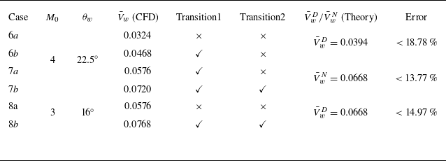
 V¯wD
 V¯wN

 V¯wD
 V¯wN

 M0=4

 RR→MR