1. INTRODUCTION
Geomagnetic map suitability is an important factor of geomagnetic navigation accuracy, and also an intrinsic property of geomagnetic area matching (Hu and Wu, Reference Hu and Wu2013). Characteristic parameters of geomagnetic maps are the basic content of suitability. However, it is poor practice to evaluate the suitability with a single characteristic parameter. At present, the research into geomagnetic map suitability focuses on the Fuzzy Decision Making (FDM) method (Wang et al., Reference Wang, Wang, Zhang and Qiao2009; Wang, Reference Wang2011; Ouazraoui et al., Reference Ouazraoui, Bourareche and Nait-Said2015; Wu et al., Reference Wu, Zhang and Lu2015), and matching area classification and scene matching (Wang, Reference Wang2011). However, the membership function of FDM is a single value, and favouring and opposing content cannot be taken into account simultaneously. Characteristic parameters are used as inputs in matching area classification methods with lots of parameters and complex computation. Scene map matching is obtained from a two-dimensional map based on camera technology, which has a different application background from a three-dimensional geomagnetic environment. Thus scene map matching cannot be used for assessing geomagnetic map suitability.
From the viewpoint of matching feature extraction, the matching parameters of a matching area are described, such as macro-relief features (standard deviation), micro-cosmic fragmentation features (information entropy, roughness, and slope variance) and some parameters in different areas are likely to be relevant and some redundant (Hu and Wu, Reference Hu and Wu2013; Fan et al., Reference Fan, You and Zhang2002). A multitude of Multiple Attribute Decision Making (MADM) methods are proposed by researchers, where FDM theory (Behbood et al., Reference Behbood, Lu, Zhang and Pedrycz2015; Fan et al., Reference Fan, You and Zhang2002; Zhang et al., Reference Zhang, Xu, Li and Wang2009) has been developed for nearly five decades in many fields, including fuzzy control, pattern recognition, intelligent systems, etc. Vague set theory has been founded for no more than 20 years, and subtle differences between the attribute values should not have a decisive role in the final scheme ranking. Therefore, an interval value is set for a single attribute; if differences in attribute values of two schemes are within the threshold value, the two schemes are considered equal. Due to its advantage with abundant information and wide applicability, vague set theory has been used widely in studying and dealing with fuzzy information problems.
The remainder of this paper is organised as follows. In Section 2, the characteristic parameters of matching suitability are analysed. In Section 3, the FDM sets an evaluation matrix to analyse geomagnetic map matching suitability, an optimisation model is established and the weight coefficient is calculated. In Section 4, vague set [t A (x), 1 − f A (x)] is constituted. t A (x) is membership function and f A (x) is non-membership function, which can be understood by voting model (Xu and Wei, Reference Xu and Wei2010). The Weighted Score Function (WSF) method is adopted to select the optimal matching area. Comparing Weighted Score Function Values (WSFVs) of different areas, the biggest value corresponds to the optimal matching area. In Section 5, the simulation results demonstrate the feasibility of vague set theory in the analysis of geomagnetic map suitability.
2. CHARACTERISTIC PARAMETERS OF THE GEOMAGNETIC MAP
Geomagnetic map accuracy is a key factor to geomagnetic navigation technology feasibility. Geomagnetic field intensities are stored as grids, and the features extracted from the magnetic map data are called characteristic parameters.
Supposing the mesh size of a certain area is M × N, where M is latitude span, N is longitude span, f(i, j) is the geomagnetic field intensity value of point (i, j), and (i, j) are latitude and longitude coordinates (ϕ, λ). The definitions of the geomagnetic features are obtained as follows.
2.1. Standard Deviation
The mean of geomagnetic intensity represents the physical distribution of the geomagnetic field quantitatively. Standard deviation (Wang and Yu, Reference Wang and Yu2015) reflects the degree of dispersion and the overall ups and downs. The standard deviation is proportional to the geomagnetic matching area suitability. The geomagnetic intensity mean of matching area
 $\bar f$
and standard deviation σ is given by
 $$\bar f = \displaystyle{1 \over {MN}}\sum\nolimits_{i = 1}^M {\sum\nolimits_{\,j = 1}^N {\,f\left( {i,\,j} \right)}} $$
 $${\rm \sigma} = \sqrt {\displaystyle{1 \over {MN - 1}}\sum\nolimits_{i = 1}^M {\sum\nolimits_{\,j = 1}^N {(\,f\left( {i,\,j} \right) - \bar f)^2}}} $$
2.2. Information Entropy
In the 1950s, Shannon introduced the concept of entropy from the discipline of thermodynamics to information theory. Information entropy (Hu and Wu, Reference Hu and Wu2013; Wang and Yu, Reference Wang and Yu2015) can be regarded as a measurement, and reflects the average amount of information. Information entropy is inversely proportional to the geomagnetic matching area suitability. With the logarithm base of 2, the entropy unit is a bit, and the information entropy H is given by
 $${\rm H} = - \sum\nolimits_{i = 1}^M {\sum\nolimits_{\,j = 1}^N {\,p\left( {i,\,j} \right) \cdot log_2\,p\left( {i,\,j} \right)}} $$
where p(i, j) is:
 $$p\left( {i,\,j} \right) = \displaystyle{{\,f\left( {i,\,j} \right)} \over {\mathop \sum \nolimits_{i = 1}^M \mathop \sum \nolimits_{\,j = 1}^N f\left( {i,\,j} \right)}}$$
Simultaneously, the amount of entropy is determined by all the geomagnetic field intensity values within local geomagnetic windows. Since a single intensity value has a small effect on entropy, discrete points can be eliminated in this way. Moreover, after being normalised, the noise can be smoothed.
2.3. Roughness
Geomagnetic roughness (Galvan-Tejada et al., Reference Galvan-Tejada, Garcia-Vazquez, Galvan-Tejada and Brena2015) reflects the smoothness and fluctuations of the local geomagnetic field. The roughness is proportional to the geomagnetic matching area suitability. r x is roughness in direction x, r y is roughness in direction y, the roughness r is given by
 $${\rm r} = \displaystyle{{r_x + r_y} \over 2}$$
 $$r_x = \sqrt {\displaystyle{1 \over {M\left( {N - 1} \right)}}\sum\nolimits_{i = 1}^M {\sum\nolimits_{\,j = 1}^{N - 1} {[\,f\left( {i,\,j} \right) - f\left( {i,\,j + 1} \right)]^2}}} $$
 $$r_y = \sqrt {\displaystyle{1 \over {N\left( {M - 1} \right)}}\sum\nolimits_{i = 1}^{M - 1} {\sum\nolimits_{\,j = 1}^N {[\,f\left( {i,\,j} \right) - f\left( {i + 1, j} \right)]^2}}} $$
2.4. Slope Variance
Geomagnetic slope (Min-Ho et al., Reference Min-Ho, Baskakov, Terechov and Kononov2013) is defined by the angle between the normal direction and the vertical direction, both on the geomagnetic field surface, and can be determined by S x (i, j) and S y (i, j).
 $$\eqalign{ S_x\left( {i,\,j} \right) &= [\,f\left( {i + 1,\,j + 1} \right) + f\left( {i,\,j + 1} \right) + f\left( {i - 1,\,j + 1} \right) \cr & \quad - f\left( {i + 1,\,j - 1} \right) - f\left( {i,\,j - 1} \right) - f\left( {i - 1,\,j - 1} \right)]} $$
 $$\eqalign{ S_y\left( {i,\,j} \right) & = [\,f\left( {i + 1,\,j + 1} \right) + f\left( {i + 1,\,j} \right) + f\left( {i + 1,\,j - 1} \right) \cr & \quad - f\left( {i - 1,\,j + 1} \right) - f\left( {i - 1,\,j} \right) - f\left( {i - 1,\,j - 1} \right)]/6} $$
The method of calculation of slope S(i, j) is given by
 $$S\left( {i,\,j} \right) = \sqrt {S_x \left( {i,\,j} \right)^2 \,+ \,S_y \left( {i,\,j} \right)^2} $$
S(i, j) reflects the overall magnetic slope of the matching area. Therefore, slope variance S σ is given by
 $$S_\sigma = \sqrt {\displaystyle{1 \over {\left( {M - 2} \right)\left( {N - 2} \right) - 1}}\sum\nolimits_{i = 2}^{M - 1} {\sum\nolimits_{\,j = 2}^{N - 1} {(S\left( {i,\,j} \right) - \bar S)^2}}} $$
3. SELECTION CRITERIA OF THE FDM METHOD
We set the number of candidate matching areas at m, and the property number is n (geomagnetic map features). The scheme evaluation matrix (Zhang et al., Reference Zhang, Xu, Li and Wang2009) X is given by
 $${\rm X} = \left[ {\matrix{ {{\rm x}_{11}} & {{\rm x}_{12}} \cr} \cdots {\rm x}_{1{\rm n}}} \right]$$
 $${\rm X} = \left[ {\matrix{ {x_{11}} & \cdots & {x_{1n}} \cr \vdots & \ddots & \vdots \cr {x_{m1}} & \cdots & {x_{mn}} \cr}} \right] = [x_{ij} ]_{m \times n} $$
 $$i = 1, 2, \ldots m;\;j = 1, 2, \ldots n$$
where x ij is the evaluation value the matching area i corresponding to property j. In the MADM, property types are divided into four types as benefit, cost, interval and fixed. Benefit types with bigger value are better, cost types with smaller values are better, and as for interval type, the property value is closer to a fixed interval with better property, and fixed type with a fixed value is better. The FDM includes the first two types.
-
(1) Benefit type, of which membership is given by
(13) $${\rm r}_{ij =} {{x_{ij}} / \!{x_{\max}}} \quad \quad i = 1, 2, \ldots m;\,j = 1, 2, \ldots n$$
x max is the maximum of x ij .
-
(2) Cost type, of which membership is given by
(14)
$${\rm r}_{ij =} {{x_{ij}} / \!{x_{\min}}} \quad \quad i = 1, 2, \ldots m;j = 1, 2, \ldots n $$
x min is the minimum of x ij .


Evaluation matrix after normalisation by Equation (13) and Equation (14)
 $${\rm R}_{m \times {\rm n}} = [r_{ij} ]_{m \times {\rm n}} \quad i = 1, 2, \ldots m;\,j = 1, 2, \ldots n$$
Setting the weight vector w = (w 1, w 2, …w n ) meets the normalisation constraint.
 $$\sum\nolimits_{\,j = 1}^n {w_j = 1}, \quad w_i \ge 0 \quad j = 1, 2, \ldots n$$
Comprehensive evaluation of the i-th matching area is V i (w)
 $${\rm V}_i \left( w \right) = \sum\nolimits_{\,j = 1}^m {w_j r_{ij}} $$
Obviously, a bigger V i (w) is better, which means a more advantageous matching performance. For a certain evaluation index, the deviation between evaluation of the scheme evaluated and others is depicted by f ij (w)
 $${\rm f}_{ij} \left( w \right) = \sum\nolimits_{k = 1}^n {w_j \left \vert {r_{ij}} \right. - \left. {r_{ik}} \right \vert} \quad j,\,k = 1, 2, \ldots n$$
The purpose of the evaluation system is to determine a reasonable indicator of the weights, and make the deviation the largest. To solve the weight coefficient, the optimisation model (Gau and Buehere, Reference Gau and Buehere1993; Odejobi et al., Reference Odejobi, Wong and Beaumont2007) is established by using Shannon information entropy.
 $$\max \quad \mu \mathop \sum \limits_{i = 1}^m \mathop \sum \limits_{\,j = 1}^n \mathop \sum \limits_{k = 1}^n w_j \left \vert {r_{ij}} \right. - \left. {r_{ik}} \right \vert - \left( {1 - \mu} \right)\mathop \sum \limits_{i = 1}^n w_j lg\;w_j $$
 $$s.t.\sum\nolimits_{\,j = 1}^n {w_j = 1}, \quad w_j \ge 0 \quad i = 1, 2, \ldots m;\,j,\,k = 1, 2, \ldots n$$
Positive parameter μ(0 < μ < 1) represents an equilibrium coefficient between two goals. According to the maximum deviations principle and maximum entropy principle, the optimisation model has a unique solution
 $$w = \left( {\displaystyle{{S_1} \over {\mathop \sum \nolimits_{\,j = 1}^n S_j}}, \displaystyle{{S_2} \over {\mathop \sum \nolimits_{\,j = 1}^n S_j}}, \cdots, \displaystyle{{S_n} \over {\mathop \sum \nolimits_{\,j = 1}^n S_j}}} \right)$$
 $$S_j = {\rm exp}\left[ {\mu \sum\nolimits_{i = 1}^m {\sum\nolimits_{k = 1}^m {\displaystyle{{\left \vert {r_{ij} - r_{kj}} \right \vert} \over {1 - \mu}} - 1}}} \right] \quad j = 1, 2, \ldots n$$
The comprehensive evaluation values of all schemes are given by
 $$\left( {V_1 \left( w \right), V_2 \left( w \right), \ldots V_n \left( w \right)} \right)^T = R \times w$$
and determine the best solution based on the comprehensive evaluation of the maximum principle.
4. ANALYSIS ON THE GEOMAGNETIC MAP SUITABILITY BASED ON VAGUE SET
Due to the membership function of a fuzzy set being a single value, favouring and opposing extent cannot be taken into account simultaneously. To this end, the vague set theory was put forward by Gau and Buehrer (Reference Gau and Buehere1993). Similarly, domain X = {x1, x 2, … x n } is composed of information features, vague set of domain X is described by a membership function and non-membership function, and the lower bound of membership t A (x i ) is derived from favouring content, the lower bound of non-membership f A (x i ) is derived from opposing content. Therefore, vague set [t A (x i ), 1 − f A (x i )] is a subinterval of interval [0, 1], denoted as V A (x i ).
 $$A = \displaystyle{{\mathop \sum \nolimits_{i = 1}^n \left[ {t_A \left( {x_i} \right), 1 - f_A \left( {x_i} \right)} \right]} \over {x_i}} \quad \quad x_i \in {\rm X}$$
Uncertainty π A (x i ) is calculated as π A (x i ) = 1 − t A (x i ) − f A (x i ), which is a measurement of unknown information. Vague set data are compared by:
-
(1)
$t_{ij} \in \left[ {0, 1} \right], 1 - f_{ij} \in \left[ {0, 1} \right]$
; -
(2)
$t_{ij} \le x_{ij} \le 1 - f_{ij} $
; -
(3)
$t_{ij} + f_{ij} \le 1$
;



4.1. Conversion Methods from Fuzzy Valued Data to Vague Valued Data
The relationship between fuzzy and vague membership functions has been extensively researched (Wang, Reference Wang2010; Wang et al., Reference Wang, Zhang and Zheng2012), three types are listed below, equation [t ij , 1 − f ij ] is converted from fuzzy valued data to vague valued data.
Method 1 Elements of domain X = [x ij ] m×n represent fuzzy set data x ij , define:
 $$t_{ij} = \left\{ {\matrix{{x_{ij} - k \quad x_{ij} - k \ge 0} \cr \quad \hskip-12pt{x_{ij}\quad \quad \quad\hskip-8pt \;\;x_{ij} - k \lt 0} \cr}} \right. 1 - f_{ij} = \left\{ {\matrix{{x_{ij} + k \quad x_{ij} + k \le 1 } \cr {x_{ij}\quad \quad \quad \!\!x_{ij} + k \gt 1} \cr}} \right. \left( {k \in \left[ {0, 1} \right]} \right)$$
Method 2 Elements of domain X = [x ij ] m×n represent fuzzy set data x ij , define:
 $$_{ij} = \left\{ {\matrix{{x_{ij} - px_{ij} \quad \! x_{ij} \ne 1} \cr {1\quad \quad \quad \quad x_{ij} = 1}\cr}} \right. 1 - f_{ij} = \left\{ {\matrix{{x_{ij} + q\left( {1 - x_{ij}} \right) x_{ij} \ne 0} \cr {0 \quad \quad \quad \quad \quad \quad \!x_{ij} = 0} \cr}} \right.\left( {\,p,\,q \in \left[ {0, 1} \right]} \right)$$
Method 3 Elements of domain X = [x ij ] m×n represent fuzzy set data x ij , define:
 $$t_{ij} = \left\{ {\matrix{ {x_{ij} - rx_{ij}\; x_{ij} - rx_{ij} \ge 0 } \cr {x_{ij} \quad \quad \quad \!x_{ij} - rx_{ij} \lt 0 } \cr } } \right.1 - f_{ij} = \left\{ {\matrix{ \hskip2pt{x_{ij} + sx_{ij} \;x_{ij} + sx_{ij} \le 1 } \cr {x_{ij} \quad \quad \quad x_{ij} + sx_{ij} \gt 1 } \cr } } \right.\left( {\,p,\,q\left[ {0, 1} \right]} \right)$$
For example, if
 $x_{ij} = 1, \left[ { t_{A_i}, 1 - f_{A_i}} \right] = \left[ {1, 1} \right], {\rm if}\,x_{ij} = 0, \forall {\rm p}, {\rm q}, \left[ { t_{A_i}, 1 - f_{A_i}} \right] = \left[ {0, 0} \right], $
 $ x_{ij}, t_{ij}, f_{ij}$
meet all vague set conditions. If
 $x_{ij} \ne 1\,and\,x_{ij} \ne 0,\,\forall {\rm p},{\rm q},\;x_{ij} - f_{ij} =$
 $x_{ij} - px_{ij} + \left[ {1 - x_{ij} - q\left( {1 - x_{ij}} \right)} \right] = 1 - px_{ij} - q\left( {1 - x_{ij}} \right) \le 1$
, and
 $x_{ij} \in \left[ {0,1} \right]$
, so
 $t_{ij} = x_{ij} - px_{ij} \in \left[ {0,1} \right], 1 - f_{ij} \in x_{ij} + q\left( {1 - x_{ij}} \right) \in \left[ {0,1} \right], x_{ij}, t_{ij}, f_{ij}$
meet all vague set conditions. Similarly, Methods 1 and 3 can be proved in the same way.
4.2. The WSF Method
Considering the comparative advantage, known information of vague set
 $\left[ { t_{A_i}, 1 - f_{A_i}} \right]$
(Wang et al., Reference Wang, Zhang and Zheng2012), the score function analysis are listed as follows.
Step 1 Vague set
 $\left[ { t_{A_i}, 1 - f_{A_i}} \right]$
, is divided into four types:
-
1) If
$t_{A_i} \gt f_{A_i} \;and\;t_{A_i} + f_{A_i} = 1$
, classified as a type, referred as T
1 =
$\left\{ {\left[ {t_{A_i}, 1 - f_{A_i}} \right]\left\vert {t_{A_i} \gt f_{A_i}\,and\,t_{A_i} + f_{A_i} = 1} \right.} \right\}$
. -
2) If
$t_{A_i} \gt f_{A_i}\,and\,t_{A_i} + f_{A_i} \lt 1$
, classified as a type, referred as T
2 =
$T_2 = \left\{ {\left[ {t_{A_i}, 1 - f_{A_i}} \right]\left\vert {t_{A_i} \gt f_{A_i}\,and\,t_{A_i} + f_{A_i} \lt 1} \right.} \right\}$
. -
3) If
$t_{A_i} = f_{A_i} $
, classified as a type, referred as
$T_3 = \left\{ {\left[ {t_{A_i}, 1 - f_{A_i}} \right]\left\vert {t_{A_i} = f_{A_i}} \right.} \right\}$
. -
4) If
$t_{A_i} \lt f_{A_i} $
, classified as a type, referred as
$T_4 = \left\{ {\left[ {t_{A_i}, 1 - f_{A_i}} \right]\left\vert {t_{A_i} \lt f_{A_i}} \right.} \right\}$
.


Step 2 For the same feature, vague set values are calculated and compared:
 $$XH \left(E \left(A_i \right) \right) = \left\{\matrix{2t_{A_i} \hfill &t_{A_i} \gt f_{A_i}\,and\,t_{A_i} + f_{A_i} = 1 \hfill \cr t_{A_i} + f_{A_i} + \left( t_{A_i} - f_{A_i} \right) \pi_{A_i} \hfill &t_{A_i} \gt f_{A_i}\,and\,t_{A_i} + f_{A_i} \lt 1 \hfill \cr - \left(t_{A_i} + f_{A_i} \right)\pi_{A_i}\hfill &t_{A_i} = f_{A_i} \hfill \cr t_{A_i} - 2f_{A_i} - \left(t_{A_i} + f_{A_i} \right) \pi_{A_i} \hfill &t_{A_i} \lt f_{A_i} \hfill} \right. $$
For a certain information feature, XH(E(Ai)) is proportional to the matching suitability, and area Ai meets the requirements of the decision makers.
Step 3 Different features C j (j = 1, 2, … n) have different influence in geomagnetic map suitability, therefore, set weight w = (w 1, w 2, …w n ), the equation of the WSF is:
 $$\eqalign{W_C \left( {A_i} \right) & = XH\left( {\left \vert {t_{i1}, 1 - f_{i1}} \right \vert} \right) \times w_1 + XH\left( {\left \vert {t_{i2}, 1 - f_{i2}} \right \vert} \right) \cr & \quad \times w_2 + \ldots + XH\left( {\left \vert {t_{in}, 1 - f_{in}} \right \vert} \right) \times w_n \quad i = 1, 2, \ldots m}$$
The suitability of area A i has been quantified by W C (A i ) with a proportional relationship.
5. SIMULATION
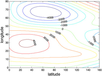
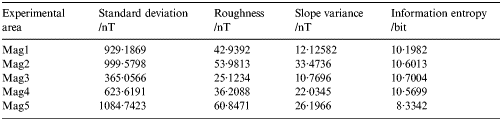
Geomagnetic data of a certain geomagnetic model are obtained as a map, and a larger evaluation value has better suitability. The best geomagnetic matching area can be determined after calculation and simulation. Figure 1 is a contour map of the geomagnetic model, geomagnetic intensities were numbered, the grid size is 401 × 401, five areas with a grid size 41 × 41 were selected as experimental maps. Table 1 is the geomagnetic map information features of experimental maps, standard deviation, roughness, slope variance and information entropy are calculated successively for the five areas.
-
1) The standard deviation, roughness and slope variance belong to the benefit index, and information entropy belongs to the cost index. Fuzzy matrix R was formed after the normalisation process.
$${\rm R} = \left[ {\matrix{ {0 \!\cdot\! 8566} & {0 \!\cdot\! 7057} & {0 \!\cdot\! 3622} & {0 \!\cdot\! 8172} \cr {0 \!\cdot\! 9215} & {0 \!\cdot\! 8872} & \!\!\!\!\!\!\!\!\!\!\!\!\!\!\!1 & {0 \!\cdot\! 7861} \cr {0 \!\cdot\! 3365} & {0 \!\cdot\! 4129} & {0 \!\cdot\! 3217} & {0 \!\cdot\! 7789} \cr {0 \!\cdot\! 5749} & {0 \!\cdot\! 5951} & {0 \!\cdot\! 6583} & {0 \!\cdot\! 7885} \cr \!\!\!\!\!\!\!\!\!\!\!\!\!\!\!1 & \!\!\!\!\!\!\!\!\!\!\!\!\!\!\!1 & {0 \!\cdot\! 7826} & \!\!\!\!\!\!\!\!\!\!\!\!\!\!\!1 \cr}} \right]$$
-
2) Setting balance coefficient μ = 0·8, weight vector was calculated by Equation (20):
$$w = \left( {0 \!\cdot\! 5630,\,0 \!\cdot\! 1682,\,0 \!\cdot\! 2600,\,0 \!\cdot\! 0088} \right)$$
-
3) According to Equation (21), comprehensive evaluation V of each area was obtained:
$$V = \left( {0 \!\cdot\! 7023,\, 0 \!\cdot\! 9349,\,0 \!\cdot\! 3494,\,0 \!\cdot\! 6019,\,0 \!\cdot\! 9435} \right)$$
Obviously, from the sorted performance of the five areas is: Mag5> Mag2> Mag1> Mag4> Mag3.
-
4) According to Methods 1–3, the single fuzzy set value had been transformed to an interval value of a vague set.
Conversion according to Method 1, k = 0·3, vague set R1:
$${\hskip-22pt\rm R}1 = \left[ {\matrix{ {\left( {0 \!\cdot\! 5566, 0 \!\cdot\! 8566} \right)} & {\left( {0 \!\cdot\! 4057, 0 \!\cdot\! 7057} \right)} & {\left( {0 \!\cdot\! 0622, 0 \!\cdot\! 6622} \right)} & {\left( {0 \!\cdot\! 5172, 0 \!\cdot\! 8172} \right)} \cr {\left( {0 \!\cdot\! 6215, 0 \!\cdot\! 9215} \right)} & {\left( {0 \!\cdot\! 5872, 0 \!\cdot\! 8872} \right)} & {\left( {0 \!\cdot\! 7, 1} \right)} & {\left( {0 \!\cdot\! 4861, 0 \!\cdot\! 7861} \right)} \cr {\left( {0 \!\cdot\! 0365, 0 \!\cdot\! 6365} \right)} & {\left( {0 \!\cdot\! 1129, 0 \!\cdot\! 7129} \right)} & {\left( {0 \!\cdot\! 0271, 0 \!\cdot\! 6217} \right)} & {\left( {0 \!\cdot\! 4789, 0 \!\cdot\! 7789} \right)} \cr {\left( {0 \!\cdot\! 2749, 0 \!\cdot\! 8749} \right)} & {\left( {0 \!\cdot\! 2951, 0 \!\cdot\! 8951} \right)} & {\left( {0 \!\cdot\! 3583, 0 \!\cdot\! 9583} \right)} & {\left( {0 \!\cdot\! 4885, 0 \!\cdot\! 7885} \right)} \cr {\left( {0 \!\cdot\! 7, 1} \right)} & {\left( {0 \!\cdot\! 7, 1} \right)} & {\left( {0 \!\cdot\! 4826, 0 \!\cdot\! 7862} \right)} & {\left( {0 \!\cdot\! 7, 1} \right)} \cr}} \right]$$
Conversion according to Method 2, p = 0·3; q = 0·5, vague set R2:
$${\hskip-22pt\rm R} 2 = \left[ {\matrix{ {\left( {0 \!\cdot\! 5996, 0 \!\cdot\! 9283} \right)} & {\left( {0 \!\cdot\! 4940, 0 \!\cdot\! 8528} \right)} & {\left( {0 \!\cdot\! 2536, 0 \!\cdot\! 6811} \right)} & {\left( {0 \!\cdot\! 5721, 0 \!\cdot\! 9086} \right)} \cr {\left( {0 \!\cdot\! 6450, 0 \!\cdot\! 9607} \right)} & {\left( {0 \!\cdot\! 6210, 0 \!\cdot\! 9436} \right)} & {\left( {1, 1} \right)} & {\left( {0 \!\cdot\! 5503, 0 \!\cdot\! 8931} \right)} \cr {\left( {0 \!\cdot\! 2356, 0 \!\cdot\! 6683} \right)} & {\left( {0 \!\cdot\! 2890, 0 \!\cdot\! 7064} \right)} & {\left( {0 \!\cdot\! 2252, 0 \!\cdot\! 6609} \right)} & {\left( {0 \!\cdot\! 5452, 0 \!\cdot\! 8894} \right)} \cr {\left( {0 \!\cdot\! 4024, 0 \!\cdot\! 7875} \right)} & {\left( {0 \!\cdot\! 4166, 0 \!\cdot\! 7975} \right)} & {\left( {0 \!\cdot\! 4608, 0 \!\cdot\! 8291} \right)} & {\left( {0 \!\cdot\! 5519, 0 \!\cdot\! 8942} \right)} \cr {\left( {1, 1} \right)} & {\left( {1, 1} \right)} & {\left( {0 \!\cdot\! 5478, 0 \!\cdot\! 8913} \right)} & {\left( {1, 1} \right)} \cr}} \right]$$
Conversion according to Method 3, r = 0·3; s = 0·45, vague set R3:
$${\hskip-22pt\rm R}3 = \left[ {\matrix{ {\left( {0 \!\cdot\! 5996, 0 \!\cdot\! 8566} \right)} & {\left({0 \!\cdot\! 4940, 0 \!\cdot\! 7057} \right)} & {\left( {0 \!\cdot\! 2536, 0 \!\cdot\! 5253} \right)} &{\left( {0 \!\cdot\! 5721, 0 \!\cdot\! 8172} \right)} \cr {\left( {0 \!\cdot\! 6450, 0 \!\cdot\! 9215} \right)}& {\left( {0 \!\cdot\! 6210, 0 \!\cdot\! 8872} \right)} & {\left( {0 \!\cdot\! 7, 1} \right)}& {\left( {0 \!\cdot\! 5503, 0 \!\cdot\! 7861} \right)} \cr {\left( {0 \!\cdot\! 2356, 0 \!\cdot\! 4880}\right)} & {\left( {0 \!\cdot\! 2890, 0 \!\cdot\! 5987} \right)} & {\left( {0 \!\cdot\! 2252, 0 \!\cdot\! 4665} \right)} & {\left( {0 \!\cdot\! 5452, 0 \!\cdot\! 7789} \right)} \cr {\left({0 \!\cdot\! 4024, 0 \!\cdot\! 8336} \right)} & {\left( {0 \!\cdot\! 4166, 0 \!\cdot\! 8629} \right)} &{\left( {0 \!\cdot\! 4608, 0 \!\cdot\! 9545} \right)} & {\left( {0 \!\cdot\! 5519, 0 \!\cdot\! 7885} \right)}\cr {\left( {0 \!\cdot\! 7, 1} \right)} & {\left( {0 \!\cdot\! 7, 1} \right)} &{\left( {0 \!\cdot\! 5478, 0 \!\cdot\! 7826} \right)} & {\left( {0 \!\cdot\! 7, 1} \right)} \cr}} \right]$$
-
5) According to the WSF method, the WSFVs of R1, R2 and R3 are obtained as Table 2:
Comparing the WSFVs under three conversion methods respectively, a same-sorted suitability was obtained: Mag5> Mag2> Mag1> Mag4> Mag3, and was consistent with the FDM result, which showed the feasibility of vague set theory.
-
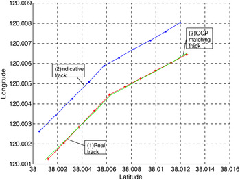
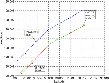
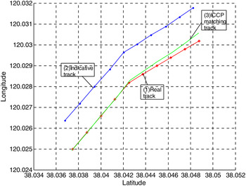
6) To explain the suitability of experimental areas, Figures 2–4 show the result that ICCP (Iterative Closest Contour Point) algorithm is used in Mag1 and Mag3 and Mag5, vertical and horizontal coordinates are latitude and longitude, respectively. Curve (1) is the real track, curve (2) is the indicative track, and curve (3) is the ICCP matching track. The same initial conditions and position error were used, and from the matching results it can be seen that the matching performance of Mag 5 was the best, followed by Mag3 and Mag1. This demonstrated that the vague set could be used to select the adapting area effectively, and also provided a numerical reference of underwater geomagnetic navigation route planning in the shortest path.


The geomagnetic contour map.

ICCP algorithm used in Mag5.

ICCP algorithm used in Mag3.

ICCP algorithm used in Mag1.

Geomagnetic map information features of five experimental maps.

The WSFVs.

6. CONCLUSIONS
Based on the FDM method, a vague set method with membership function and non-membership function has been presented. The advantages of this vague set method on geomagnetic matching area selection are analysed theoretically, and the consistency of evaluation values obtained by the vague set method is verified by simulation results and ICCP method. In practical application, the proposed approach is a viable solution to solve problems of one-sided appraisal in selecting matching area, and optimising selection of the geomagnetic-aided navigation area. In current work, vague set data are obtained from conversion formulae, and the suitability rank is the same compared with the FDM. The succeeding work is planning to obtain vague set data from geomagnetic map features directly, and all these uncertain facts should be considered into a fixed interval, such as geomagnetic fluctuation, noise, measurement error, etc. Conversion formulae from fuzzy set data to vague set data will be surplus to requirements, and vague set data are more accurate.
ACKNOWLEDGEMENTS
The project is supported by the following funds: National Natural Science Foundation of China (61203192, 51477028), Research Fund of China Ship Industry (13J3·8·4), Foundation of Key Laboratory of Micro-Inertial Instrument and Advanced Navigation Technology, Ministry of Education (201103).