1. Introduction
Many planetary bodies in our solar system consist of a solid inner and a liquid outer core, e.g. the Earth, Mercury, Jupiter and Saturn as planets but also satellites like the Earth’s moon and the Galilean moons of Jupiter. Most of them do not rotate at a constant speed but undergo superposed oscillations on the mean rotation (called longitudinal librations) due to interactions with their gravitational partners (Comstock & Bills Reference Comstock and Bills2003; Spohn Reference Spohn and Schubert2007; Noir et al. Reference Noir, Hemmerlin, Wicht, Baca and Aurnou2009). The Earth’s core, on the other hand, undergoes differential rotation where the inner core and outer mantle are rotating at different speeds. This happens due to a strong gravitational coupling between mantle and inner core where small fluctuations of the mantle momentum have a strong impact on the inner core’s rotation (Aldridge & Lumb Reference Aldridge and Lumb1987; Rieutord Reference Rieutord1995). But, also, accretion disks are driven by differential rotation (Li et al. Reference Li, Finn, Lovelace and Colgate2000, Reference Li, Colgate, Wendroff and Liska2001). All these rotational background systems have a significant influence on the liquid interior of planets and stars. It is worth knowing the interaction between the core rotation and the interior of the fluid to understand e.g. tidal heating, fluid mixing and the generation of magnetic fields. Inertial waves (e.g. in the Earth’s liquid outer core Aldridge & Lumb Reference Aldridge and Lumb1987; Rieutord Reference Rieutord1995) and Stewartson shear layers (Stewartson Reference Stewartson1957, Reference Stewartson1966; Hide & Titman Reference Hide and Titman1967; Früh & Read Reference Früh and Read1999; Hollerbach Reference Hollerbach2003; Koch et al. Reference Koch, Harlander, Egbers and Hollerbach2013; Sauret & Le Dizès Reference Sauret and Le Dizès2013) are two flow phenomena excited by such background rotations. Of particular interest are wave interactions and Stewartson-layer instabilities (Hide & Titman Reference Hide and Titman1967; Hollerbach Reference Hollerbach2003; Hollerbach et al. Reference Hollerbach, Futterer, More and Egbers2004; Schaeffer & Cardin Reference Schaeffer and Cardin2005a ,Reference Schaeffer and Cardin b ; Wicht Reference Wicht2014).
An opportunity to explore aspects of the dynamics and mechanisms in planets and stars is to do laboratory experiments. The first experiments of this type were done by Aldridge & Toomre (Reference Aldridge and Toomre1969) in a librating full sphere. The results of this work show good agreement with the expected global eigenmodes (Rieutord Reference Rieutord1991). Later, Aldridge (Reference Aldridge1972) reported that similar eigenmodes also exist in thick spherical shells. However, the interpretation of these findings has been revised and clarified by Zhang et al. (Reference Zhang, Chan, Liao and Aurnou2013). The apparatus in our study is able to do both differential rotation and inner sphere libration. In this work, the latter has been used to study inertial waves, wave interactions and instabilities under controllable forcing conditions (Koch et al. Reference Koch, Harlander, Egbers and Hollerbach2013). Of special interest is the wave-reflection behaviour at inclined walls, which can be studied using simple ray models (Greenspan Reference Greenspan1968; Tilgner Reference Tilgner1999; Harlander & Maas Reference Harlander and Maas2006; Borcia & Harlander Reference Borcia and Harlander2013; Koch et al. Reference Koch, Harlander, Egbers and Hollerbach2013). From such models, but also from experiments and numerical simulations, it is known that for spherical shells energy can be focused on closed orbits and wave attractors (Tilgner Reference Tilgner1999; Maas Reference Maas2001; Rieutord, Georgeot & Valdettaro Reference Rieutord, Georgeot and Valdettaro2001; Harlander & Maas Reference Harlander and Maas2006; Rabitti & Maas Reference Rabitti and Maas2013, Reference Rabitti and Maas2014).
Further, similar to differential rotation, inner sphere libration gives rise to a Stewartson layer. Note that, in contrast to the classical Stewartson layer, the libration-induced Stewartson layer appears in the form of a prograde jet. Recent experimental and numerical studies about these jet-like layers can be found in Koch et al. (Reference Koch, Harlander, Egbers and Hollerbach2013), Sauret & Le Dizès (Reference Sauret and Le Dizès2013), Klein et al. (Reference Klein, Seelig, Kurgansky, Ghasemi V., Borcia, Will, Schaller, Egbers and Harlander2014) and Seelig (Reference Seelig2014). In the context of a spherical shell, the Stewartson layer forms a vertical cylinder parallel to the axis of rotation touching the inner sphere’s equator (Stewartson Reference Stewartson1957, Reference Stewartson1966; Hollerbach Reference Hollerbach2003; Koch et al. Reference Koch, Harlander, Egbers and Hollerbach2013; Sauret & Le Dizès Reference Sauret and Le Dizès2013). For a critical shear, e.g. when the libration amplitude or the differential rotation exceeds a certain threshold, this layer becomes unstable. Such shear-flow instabilities are of general geophysical interest, e.g. in meteorology (barotropic Rossby waves), oceanography (gulf stream) and astrophysics (Jovian jet).
Laboratory experiments on Stewartson layers have previously been performed in cylindrical cavities by Hide & Titman (Reference Hide and Titman1967), who used a differentially rotating disk at half height of the tank, and Früh & Read (Reference Früh and Read1999), who used differentially rotating disks in the top and bottom lids to excite Stewartson layers. In case of super-rotation, where the disks are rotating faster than the cylinder, both experiments exhibit an increasing azimuthal wavenumber
 $m$
of the instabilities with decreasing Ekman number
 $E\sim {\it\Omega}^{-1}$
. In case of subrotation, Früh & Read (Reference Früh and Read1999) found the same behaviour of the wavenumber but Hide & Titman (Reference Hide and Titman1967) reported a ‘mysterious’
 $m=1$
mode that is nearly independent of
 $E$
. With the exception of this
 $m=1$
mode, which could not be confirmed by other experiments to date, both experiments are in qualitative agreement with the linear stability analysis of Busse (Reference Busse1968). For cylindrical geometry, he found that a critical differential Rossby number of
 $Ro_{d,crit}\sim E^{3/4}$
, with
 $Ro_{d}=({\it\Omega}_{i}-{\it\Omega}_{o})/{\it\Omega}_{o}$
, must be exceeded for the onset of Stewartson-layer instabilities. Further, he found that there are no differences between positive and negative
 $Ro_{d}$
.
Referring to the two experiments by Hide & Titman (Reference Hide and Titman1967) and Früh & Read (Reference Früh and Read1999), Hollerbach (Reference Hollerbach2003) and Hollerbach et al. (Reference Hollerbach, Futterer, More and Egbers2004) presented experimental and direct numerical solutions considering the instability of the Stewartson layer in spherical rather than cylindrical geometry. Based on a rapidly rotating spherical shell with imposed small differential rotation on the inner sphere, Hollerbach (Reference Hollerbach2003) systematically analysed the wavenumber of the instabilities depending on the sign of
 $Ro_{d}$
. He found that the structure of the Stewartson layer does not contribute to the differences in the wavenumbers between positive and negative
 $Ro_{d}$
. However, the geometry itself has the most significant influence on the instabilities. By comparing a full sphere, a thin spherical shell and a spherical shell with
 $r_{i}=0.5$
, he found that neither a constant nor a monotonically decreasing/increasing fluid height does contribute to the wavenumber differences. But, when the height is changing abruptly by crossing the tangent cylinder, the
 $Ro_{d}<0$
case becomes different to the
 $Ro_{d}>0$
case, i.e. the
 $m=1$
mode appears for
 $Ro_{d}<0$
. To pin down the reason for the difference, he studied the conservation of potential vorticity and found that in the case of a spherical shell, a discontinuity in potential vorticity occurs at
 $r_{i}$
for negative
 $Ro_{d}$
, explaining the differences between positive and negative
 $Ro_{d}$
.
Based on the findings by Hollerbach (Reference Hollerbach2003), Schaeffer & Cardin (Reference Schaeffer and Cardin2005a
,Reference Schaeffer and Cardin
b
) developed a quasigeostrophic (QG) model to analyse so-called Rossby-wave instabilities of the Stewartson layer depending on different geometries. They studied a flat container with
 ${\it\beta}=0$
, where
 ${\it\beta}=(1/L)(\text{d}L/\text{d}r)$
is the
 ${\it\beta}$
-parameter and
 $L$
the height of the container, a container with exponential shape with
 ${\it\beta}=-1$
, a split sphere with integrated polar caps of radius
 $r_{0}=0.35$
, where
 ${\it\beta}={\it\beta}(r)$
, and a sphere with flat disks of radius
 $r_{0}=0.35$
slightly below/above the upper/lower boundary to include a height jump at
 $r_{0}$
. They found an instability threshold of
 $Ro_{d,crit}\sim {\it\beta}E^{1/2}$
. For spherical geometry, where
 ${\it\beta}$
is a continuous function of radius
 $r$
, the
 $Ro_{d}<0$
case shows prograde drifting waves that are trapped near the tangent cylinder at
 $r=r_{0}$
. In contrast, the
 $Ro_{d}>0$
case shows prograde drifting spiral-shaped waves filling the entire gap
 $r>r_{0}$
. They can be explained by a continuously decreasing
 ${\it\beta}$
due to a decreasing fluid depth towards the outer boundary. Such spiral-shaped waves have also been found experimentally by Egbers & Rath (Reference Egbers and Rath1995) and numerically by Hollerbach, Junk & Egbers (Reference Hollerbach, Junk and Egbers2006) considering only inner sphere rotation. The spherical geometry with flat differentially rotating disks leads to a discontinuity in
 ${\it\beta}$
. In this case, Schaeffer & Cardin (Reference Schaeffer and Cardin2005a
) found, in agreement with Hollerbach (Reference Hollerbach2003), smaller wavenumbers for
 $Ro_{d}<0$
than for
 $Ro_{d}>0$
. Unfortunately, due to the discontinuity in
 ${\it\beta}(r_{i})$
, the QG model from Schaeffer & Cardin (Reference Schaeffer and Cardin2005a
) was not suitable to simulate spherical shell geometry. However, due to different signs of
 ${\it\beta}$
for
 $r<r_{i}$
and
 $r>r_{i}$
, they expected retrograde instead of prograde drifting modes in the
 $Ro_{d}<0$
case.
Later, Aguiar & Read (Reference Aguiar and Read2006) extended the experimental setup of Früh & Read (Reference Früh and Read1999) by including a height-variable upper disk in a flat cylindrical container. Their goal was to investigate the influence of the height jump on the Stewartson-layer instabilities experimentally. They found a weak spiral structure similar to that of Schaeffer & Cardin (Reference Schaeffer and Cardin2005a
) and small differences in the azimuthal wavenumber between positive and negative
 $Ro_{d}$
. Further, the differences become larger for increasing height changes and the instability structure depends on the sign of the height change.
Most recently, Wicht (Reference Wicht2014) numerically explored several forms of instabilities and flow regimes in a differentially rotating spherical shell depending on the rotation rate
 ${\it\Omega}$
, the magnitude of differential rotation
 $|{\rm\Delta}{\it\Omega}|$
as well as the sign of
 $Ro_{d}$
. In the fast-rotation regime, where Coriolis forces dominate the flow, the Stewartson layer was the source of instabilities. He detected Rossby modes in a parameter range that is also covered by our inner sphere libration experiments. In this regime, he further found strong differences in the azimuthal wavenumber between positive and negative
 $Ro_{d}$
, in agreement with findings by Hollerbach (Reference Hollerbach2003). For the
 $Ro_{d}<0$
case, the Rossby modes are characterised by nearly
 $z$
-invariant columnar patterns with a balance between pressure-gradient force and Coriolis force resulting in a slow drift. Therefore, the columnar Rossby modes can be interpreted as slow inertial modes (Wicht Reference Wicht2014). In accordance with the expectations of Schaeffer & Cardin (Reference Schaeffer and Cardin2005a
), Wicht (Reference Wicht2014) reported a prograde drift in a full sphere and a retrograde drift in a spherical shell for
 $Ro_{d}<0$
.
The main purpose of the present work is to investigate Stewartson-layer instabilities experimentally in a spherical shell excited by inner sphere libration. We start by discussing the linear regime of forced inertial waves. There is a good agreement between qualitatively and quantitatively measured inertial waves and the predicted ray structure of the ray-tracing model. In the ‘supercritical’ regime, we found a large spectrum of azimuthal wavenumbers within a parameter range where the libration amplitudes/frequencies are sufficiently large/low to excite Stewartson-layer instabilities. Their typical structures were found to be, on the one hand, spiral waves resembling the modes found by Schaeffer & Cardin (Reference Schaeffer and Cardin2005a
) for
 $Ro_{d}>0$
, and on the other hand trapped waves resembling the modes found by Hollerbach (Reference Hollerbach2003), Schaeffer & Cardin (Reference Schaeffer and Cardin2005a
) and Wicht (Reference Wicht2014) for
 $Ro_{d}<0$
. We can further confirm the differences in the azimuthal wavenumber between the
 $Ro_{d}>0$
and
 $Ro_{d}<0$
cases, where, for the
 $Ro_{d}>0$
case, the azimuthal wavenumber increases with decreasing Ekman number.
The paper is organised as follows: in § 2, we start with a description of the experimental setup and the post-processing of the raw data. In § 3, linear inertial waves will be discussed by comparing qualitative and quantitative measurements with a two-dimensional (2D) ray-tracing model. Here, we further discuss the structure of the Stewartson layer depending on the libration parameters. In § 4, we illustrate the transition to turbulence followed by a detailed discussion of the spatial structure of the low-frequency wave-like Stewartson instabilities based on particle image velocimetry data in the corotating frame. Finally, concluding remarks will be made in § 5.
2. Experimental description and data
2.1. Experimental setup
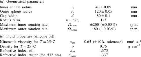
The experimental apparatus consists of an anodised aluminium inner sphere suspended on a shaft of diameter 14 mm inside an acrylic outer spherical shell (a more detailed description can be found in Koch et al. Reference Koch, Harlander, Egbers and Hollerbach2013). The working fluid, filled in the gap, is a silicone oil (‘Korasilon oil M 0.65’). All relevant parameters and fluid properties are summarised in table 1.
Geometrical and experimental parameters of the spherical shell experiment.

The shell is immersed into a cubic tank of deionised water. This helps to keep the surrounding temperature uniform and to correct optical distortion due to the curvature of the outer shell. The entire shell rotates with a mean rotation rate
 ${\it\Omega}_{0}$
. The inner sphere’s rotation undergoes an additional oscillation
 $$\begin{eqnarray}{\it\Omega}_{i}(t)={\it\Omega}_{0}+{\it\epsilon}_{lib}\cos ({\it\omega}_{lib}t),\end{eqnarray}$$
where
 ${\it\epsilon}_{lib}$
and
 ${\it\omega}_{lib}$
are the inner sphere’s libration amplitude and frequency. We can control
 $\hat{{\it\omega}}_{lib}={\it\omega}_{lib}/{\it\Omega}_{0}$
and
 $Ro_{lib}=\hat{{\it\epsilon}}_{lib}={\it\epsilon}_{lib}/{\it\Omega}_{0}$
in the ranges
 $0<\hat{{\it\omega}}_{lib}<2.0$
and
 $0<\hat{{\it\epsilon}}_{lib}\leqslant 1.0$
, respectively, with an accuracy of 0.03 %. An Ekman number of
 $E={\it\nu}_{kin}/({\it\Omega}_{0}\,d^{2})\geqslant 1.6\times 10^{-5}$
, where
 $d=r_{o}-r_{i}$
and
 ${\it\nu}_{kin}=0.65~\text{mm}^{2}~\text{s}^{-1}$
is the kinematic viscosity, can be achieved with the present configuration. In the following,
 $\hat{{\it\omega}}_{lib}$
will be used for the libration frequency and
 $\hat{{\it\omega}}$
for other frequencies in the flow. For differential rotation, where the inner and outer spheres are rotating at different speeds, a specific Rossby number
 $Ro_{d}$
is defined as
 $Ro_{d}=({\it\Omega}_{i}-{\it\Omega}_{o})/{\it\Omega}_{o}$
. In case of maximum inner sphere libration with
 $Ro_{lib}=\hat{{\it\epsilon}}_{lib}=1.0$
, the differential Rossby number
 $Ro_{d}$
varies sinusoidal in time over
 $-1\leqslant Ro_{d}\leqslant 1$
. The variation of
 $Ro_{d}$
will become important to interpret the Stewartson-layer instabilities discussed in § 4.
For visualisation in the meridional plane, the flow was seeded by Kalliroscope tracer particles and illuminated using a vertical laser light sheet. A camera recorded the flow in the laboratory frame. In addition, the flow in the horizontal plane has been studied quantitatively with particle image velocimetry (PIV). For this, a ‘GoPro Hero 3+’ camera, mounted above the sphere, enables wireless high-resolution recordings in the corotating frame. With this setup, about 50 % of the horizontal plane can be observed.
2.2. Data and data processing
We start by briefly describing the experimental procedure for Kalliroscope and PIV measurements. For a visualisation in the meridional plane, the Kalliroscope particles have been mixed by rapid inner sphere rotation. The spin-up time from rest
 $({\sim}E^{-1/2}{\it\Omega}_{0}^{-1})$
for the present configuration is about 62 and 45 s for
 ${\it\Omega}_{0}=24.4$
rounds per minute (r.p.m.) and
 ${\it\Omega}_{0}=47.8$
r.p.m., respectively. Therefore, the experiment was running for about 5 min at
 ${\it\Omega}_{0}$
in order to avoid transient spin-up recirculation and to achieve solid-body rotation. After setting the libration parameters
 $\hat{{\it\omega}}_{lib}$
and
 $\hat{{\it\epsilon}}_{lib}$
, an additional period of about 5 min is required to ensure an equilibrium state. A video of the vertical laser plane has been recorded in the laboratory frame. Note that the density of the Kalliroscope particles is somewhat larger than that of the used silicone oil. Most of the particles sediment after 15–20 min, which marks the upper limit of experimental time. The procedure for measuring in the horizontal plane differs because the spherical PIV tracer particles are floating in the silicone oil. After mixing and setting
 ${\it\Omega}_{0}$
, we waited 10 min and then set the libration frequency
 $\hat{{\it\omega}}_{lib}$
. After a transient period, we slowly increased the libration amplitude
 $\hat{{\it\epsilon}}_{lib}$
towards the maximum of
 $\hat{{\it\epsilon}}_{lib}=1.0$
. For PIV, videos have been recorded in the corotating frame.
Based on this procedure, several experiments in the parameter ranges
 $0.1\leqslant \hat{{\it\omega}}_{lib}\leqslant 1.6$
and
 $0.1\leqslant \hat{{\it\epsilon}}_{lib}\leqslant 1.0$
with increment 0.1 have been performed with a meridional laser plane. For each measurement in the meridional plane, a video of 5 min was recorded and converted into grey-scale images. A weighted average for pixel segments of
 $3\times 3$
was applied to reduce the size of the images. All regions outside the gap were masked to further reduce the amount of data. After the preprocessing, the total number of pixels in the gap is about 50 000. A harmonic analysis was applied to the time series at each pixel in the gap. The harmonic analysis is a signal demodulation in which the user specifies frequencies to be analysed and applies least-square techniques to solve for the constituents (see e.g. Emery & Thomson Reference Emery and Thomson2001, chapter 5.5). Usually, we examine the libration frequency
 $\hat{{\it\omega}}_{lib}$
and all the higher harmonics
 $k\hat{{\it\omega}}_{lib}$
included in the inertial wave frequency range (Koch et al.
Reference Koch, Harlander, Egbers and Hollerbach2013).
A subset of parameters given above has then been chosen for PIV measurements in the horizontal plane. The horizontally recorded frames have been analysed by using the Matlab toolbox ‘matPIV v. 1.6.1’ (Sveen Reference Sveen2004). For the present purpose, a spatial resolution of
 $1920\times 1080$
pixels and a frame rate of 12 frames per second were sufficient to obtain reliable velocity fields. We used three interrogation steps from
 $64\times 64$
to
 $32\times 32$
to a final window size of
 $16\times 16$
with an overlap of 0.5. A signal-to-noise filter, a peak-height filter and a global filter that removes vectors significantly larger or smaller than the majority of the vectors have further been applied. A Fourier analysis was applied to the velocity components
 $(u,v)$
to get an overview over dominant frequencies in the flow. For these frequencies, the corresponding flow patterns have been studied by harmonic analyses.
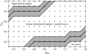
Three flow regimes can be observed: the ‘no waves’ (○), the ‘linear’ (
 $\times$
), where mainly inertial waves occur, and the ‘supercritical’ regime (
 $\star$
), where e.g. Görtler vortices and instabilities of the Stewartson layer start to grow. The uncertainty of the transitions is in the order of
 $(\hat{{\it\omega}}_{lib},\hat{{\it\epsilon}}_{lib})\sim \pm 0.1$
(grey-shaded areas). A representative Kalliroscope visualisation for each regime can be found in the supplementary material.

Figure 1 shows a regime diagram based on the data from the meridional plane. All experiments, marked as symbols, have been performed separately with an Ekman number
 $E\approx 4\times 10^{-5}$
for
 ${\it\Omega}_{0}\approx 24.4~\text{r.p.m}$
. The different regimes have usually been found by visual inspection. However, for larger libration frequencies, a complex empirical orthogonal function (CEOF) decomposition method was used to categorise the flow (Harlander et al.
Reference Harlander, Larcher, Wright, Hoff, Alexandrov, Egbers, Larcher and Williams2014). Whenever we detected homogeneous reflection, clear inertial wave shear layers or a fluctuating Stewartson layer (representative Kalliroscope visualisations can be found in the supplementary material, available at http://dx.doi.org/10.1017/jfm.2015.743), we called the regimes ‘no waves’ regime (○) (nearly solid body rotation), ‘linear regime’ (
 $\times$
) or ‘supercritical regime’ (
 $\star$
), respectively. Therefore, figure 1 is separated into three main parts. The uncertainty is represented by the grey-shaded areas. First, for small
 $\hat{{\it\epsilon}}_{lib}$
and high
 $\hat{{\it\omega}}_{lib}$
, no waves can be detected. This regime is dominated by nearly solid body rotation since the wave excitation is too weak (see appendix A). The linear regime, where inertial waves dominate the flow, forms the largest part of the diagram. A discussion of linear inertial waves is the content of the first part of the present work (§ 3). Note that also nonlinear wave–wave interactions (e.g. higher harmonics) are part of this regime (Koch et al.
Reference Koch, Harlander, Egbers and Hollerbach2013). For high
 $\hat{{\it\epsilon}}_{lib}$
and small
 $\hat{{\it\omega}}_{lib}$
, the flow becomes inertially unstable. Görtler vortices build up (see Koch et al.
Reference Koch, Harlander, Egbers and Hollerbach2013) and instabilities of the Stewartson layer start to grow. This so-called ‘supercritical’ regime (see e.g. Sauret et al.
Reference Sauret, Cébron, Le Bars and Le Dizès2012; Sauret, Cébron & Le Bars Reference Sauret, Cébron and Le Bars2013) is dominated by nonlinear flow features of interacting inertial waves and it will be the content of the second part of the present work (§ 4).
3. Linear flow features – inertial waves
We start by discussing linear inertial waves. To find the most relevant frequencies, we use a simple 2D ray-tracing model in the meridional plane of the spherical shell and compare the results with experimental data of both the meridional and the horizontal planes. Ray tracing is a method which helps to obtain a geometrical picture of the wave propagation. This method is common for hyperbolic boundary value problems (Maas Reference Maas2001; Manders & Maas Reference Manders and Maas2003; Harlander & Maas Reference Harlander and Maas2007a ,Reference Harlander and Maas b ; Borcia & Harlander Reference Borcia and Harlander2013). For the spherical shell, ray tracing has been used by Tilgner (Reference Tilgner1999), Rieutord et al. (Reference Rieutord, Georgeot and Valdettaro2001) and Rabitti & Maas (Reference Rabitti and Maas2013, Reference Rabitti and Maas2014), where the latter used a more complex 3D model.
3.1. Inertial wave beams in the meridional plane
In this section, we focus on the meridional plane. Note that our ray-tracing model is a pure geometrical mapping of straight inertial wave characteristics in spherical shell geometry. Reflections have been done by extracting the correct reflection point and changing the sign of the slope of the rays. In corners, the rays will be reflected back with the same slope. The ray-tracing model also includes the shaft of 14 mm diameter that is a boundary where waves can be reflected (see figure 2). Usually, the shear layers of the inertial waves are symmetrically excited at the ‘critical’ latitude
 ${\it\vartheta}_{c}$
in the northern and southern hemispheres, propagating northward and southward tangential to the ‘critical’ point of the inner sphere (Kerswell Reference Kerswell1995; Tilgner Reference Tilgner1999). In case of a librating spherical shell, the ‘critical’ latitude can be found from
 $$\begin{eqnarray}\sin {\it\vartheta}_{c}=\pm \hat{{\it\omega}}/2.\end{eqnarray}$$
The frequency
 $\hat{{\it\omega}}$
of the inertial waves is described by the dispersion relation
 $$\begin{eqnarray}\hat{{\it\omega}}=\frac{{\it\omega}}{{\it\Omega}_{0}}=2\sqrt{\frac{m^{2}}{k^{2}+l^{2}+m^{2}}}=2\cos {\it\theta},\end{eqnarray}$$
where
 $\boldsymbol{k}=(k,l,m)$
is the wave vector and
 ${\it\theta}$
is the angle between the group velocity
 $\boldsymbol{c}_{\boldsymbol{g}}=\partial {\it\omega}/\partial \boldsymbol{k}$
and the horizontal plane. It is remarkable that the frequency of the inertial waves does not depend on the magnitude of the wave vector but only on its direction. Inertial waves share this property with internal gravity waves. The wave rays can be approximated by straight lines (Tilgner Reference Tilgner1999; Harlander & Maas Reference Harlander and Maas2006; Borcia & Harlander Reference Borcia and Harlander2013). The inertial wave group velocity, and hence the shear layers, are perpendicular to
 $\boldsymbol{k}$
and point in the direction of energy propagation (Greenspan Reference Greenspan1968). From (3.2), it is obvious that inertial waves exist only in the range
 $0\leqslant \hat{{\it\omega}}\leqslant 2$
. For low frequencies,
 ${\it\theta}$
tends to 90° and the shear layer becomes vertical. For high frequencies,
 ${\it\theta}$
tends to 0° and the shear layer becomes horizontal. Details on the thickness of the shear layers, their reflections and velocity magnitudes for outer/inner sphere libration can be found in Kerswell (Reference Kerswell1995) and Koch et al. (Reference Koch, Harlander, Egbers and Hollerbach2013) and for a rapidly rotating and weakly precessing sphere in Kida (Reference Kida2011).
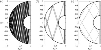
Ray paths for three different frequencies. Plotted are the last 500 of an overall number of 5000 reflections. (a)
 $\hat{{\it\omega}}=0.330$
, (b)
 $\hat{{\it\omega}}=0.604$
, (c)
 $\hat{{\it\omega}}=1.022$
.

When a ray is reflected at a boundary, the angles of incidence and of reflection are equal with respect to the rotation axis (Maas Reference Maas2001). Therefore, rays can be focused on attractors or closed orbits due to multiple reflections. The geometric pattern of the orbits depends on the inertial wave frequency
 $\hat{{\it\omega}}$
. Figure 2 shows examples of such orbits for three different frequencies
 $\hat{{\it\omega}}=(0.330,0.604,1.022)$
. From a total of 5000 reflections, we plotted just the last 500. For each case, one ray starts at the ‘critical’ latitude
 ${\it\vartheta}_{c}$
of the inner sphere in the northern hemisphere pointing in the northward direction. Obviously, for the last 500 reflections, the number of distinct reflection points depends on the frequency. Case (a) for
 $\hat{{\it\omega}}=0.330$
shows a complex structure with many different reflection points at the boundaries. In contrast, (b) and (c) for
 $\hat{{\it\omega}}=0.604$
and
 $\hat{{\it\omega}}=1.022$
show cases where the rays follow rather simple closed paths. Additionally, the orbits have branches that are close to the ‘critical’ point where the rays initially start.
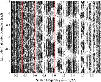
Extracting the last 500 reflection points out of a total of 5000 at the outer boundary and plotting them against the frequency
 $\hat{{\it\omega}}$
in the range
 $0<\hat{{\it\omega}}<2$
gives a so-called Poincaré plot (figure 3). The abscissa represents the dimensionless frequency
 $\hat{{\it\omega}}$
with a resolution of
 ${\rm\Delta}\hat{{\it\omega}}=0.002$
and the ordinate the latitude
 ${\it\vartheta}$
of reflection points at the outer sphere in the range
 $-{\rm\pi}/2\leqslant {\it\vartheta}\leqslant {\rm\pi}/2$
. Note that a Poincaré plot for the southward direction shows slightly different results. Especially, the attractor near
 $\hat{{\it\omega}}=1.5$
has its symmetry in the southern hemisphere. Dark regions in figure 3 represent complex ray path structures with many distinct reflection points (see e.g. figure 2
a). Such regions are the most dominant part in the diagram for the aspect ratio used. For some frequencies, ‘windows’ with fewer reflection points can be seen. These correspond to simpler ray path structures (see e.g. figure 2
b,c) that are related to attractors or closed orbits (Tilgner Reference Tilgner1999). Note that the frequencies
 $\hat{{\it\omega}}=(2\sin ({\rm\pi}/6),2\sin ({\rm\pi}/4),2\sin ({\rm\pi}/3))$
are associated with strictly periodic orbits when considering the shell without a shaft (Rieutord et al.
Reference Rieutord, Georgeot and Valdettaro2001). In our setup, the shaft of diameter 14 mm leads to a frequency shift of the periodic orbits.
Poincaré plot for ray-tracing method. Starting point is the ‘critical’ latitude
 ${\it\vartheta}_{c}$
in the northern hemisphere and the ray points in the northward direction. The dots mark reflection points at the outer sphere at position
 ${\it\vartheta}$
in radians as a function of
 $\hat{{\it\omega}}$
. 5000 reflections have been done and the last 500 are plotted against the libration frequency. The resolution is
 ${\rm\Delta}\hat{{\it\omega}}=0.002$
. The red lines mark the three frequencies depicted in figure 2.

Wave phases in the interval
 $[-{\rm\pi},{\rm\pi}]$
of a harmonic analysis for different libration parameter settings. The Ekman number is
 $E\approx 4\times 10^{-5}$
.

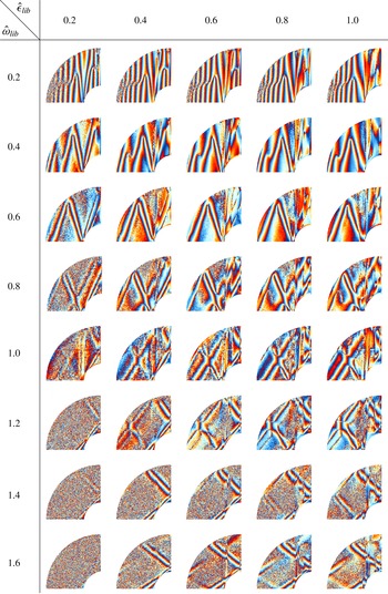
Figure 4 shows phases of the inertial wave shear layers obtained via a harmonic analysis for a parameter set
 $0.2\leqslant \hat{{\it\omega}}_{lib}\leqslant 1.6$
and
 $0.2\leqslant \hat{{\it\epsilon}}_{lib}\leqslant 1.0$
with increments of
 $({\rm\Delta}\hat{{\it\omega}}_{lib},{\rm\Delta}\hat{{\it\epsilon}}_{lib})=0.2$
. The harmonic analysis has been done for the respective libration frequency
 $\hat{{\it\omega}}_{lib}$
used to excite the corresponding inertial waves. Almost all pictures in figure 4 show shear layers approximately following straight lines, excited at the ‘critical’ point
 ${\it\vartheta}_{c}$
tangential to the inner sphere. The latter can easily be identified especially for the larger frequencies for which
 ${\it\vartheta}_{c}$
moves towards the north pole. Note that the shear layers are emitted north and southward simultaneously. Consistent with the dispersion relation (3.2) of plane inertial waves, the slope of the shear layers changes from steep to flat with increasing frequency. It can be seen that for frequencies
 $\hat{{\it\omega}}_{lib}\geqslant 1.2$
larger libration amplitudes are required to excite clear shear layers. This is for some part due to the visualisation technique, since the Kalliroscope tracer cannot follow the flow for low/high libration amplitudes/frequencies (Koch et al.
Reference Koch, Harlander, Egbers and Hollerbach2013). On the other hand, the excitation efficiency decreases with increasing frequency since the libration mechanism (2.1) becomes less effective. For higher frequencies, the excursion of the inner sphere in the corotating frame is thus smaller than for a lower frequency and the mechanism of pushing the fluid particles out of their rest positions is less efficient (see appendix A).
It can be seen that for low frequencies (
 $\hat{{\it\omega}}_{lib}\leqslant 0.6$
) there are many reflections at the outer boundary. Switching to higher frequencies, the number of reflections is reduced and it seems that the shear layers form diamond-shaped patterns that look similar to attractors. In general, it is hard to distinguish between attractors and continuously excited inertial wave rays originating tangential at the inner sphere since the latter are rather prominent in the shown pictures.
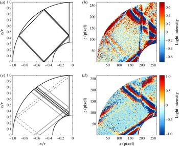
Comparison between analysed data and ray tracing in the meridional plane. (a,c) Show rays after 50 reflections for
 $\hat{{\it\omega}}=1.382$
and
 $\hat{{\it\omega}}=1.570$
, respectively. The continuous lines are excited at the northern ‘critical’ latitude and the dotted lines at the southern ‘critical’ latitude. (b,d) Show reconstructed flow fields for frequencies
 $\hat{{\it\omega}}_{lib}=1.4$
and
 $\hat{{\it\omega}}_{lib}=1.6$
, respectively. The colours represent the light intensity.

It is worth taking a closer look at particular features covered by the images in figure 4. For this, figure 5 compares two examples from figure 4 for frequencies
 $\hat{{\it\omega}}_{lib}=1.4$
,
 $\hat{{\it\epsilon}}_{lib}=0.8$
(b) and
 $\hat{{\it\omega}}_{lib}=1.6$
,
 $\hat{{\it\epsilon}}_{lib}=0.6$
(d) with ray-tracing results for similar frequencies
 $\hat{{\it\omega}}=1.382$
(a) and
 $\hat{{\it\omega}}=1.570$
(c), respectively. It should be noted that the maps of characteristics (a,c) result from a simplified model ignoring e.g. curvature, mean flows and the existence of boundary layers. It has been shown by Borcia, Ghasemi & Harlander (Reference Borcia, Ghasemi and Harlander2014) that the latter has an impact on the resonant frequencies (see table 1 in Borcia et al. (Reference Borcia, Ghasemi and Harlander2014)). Hence, there is some uncertainty about the resonant frequencies that result from the maps of characteristics. Therefore, we have chosen the frequencies that fit best to the observations even if they do not match exactly with the experimental frequencies 1.4 and 1.6 (the characteristics of the exact frequencies can be found in the supplementary material). The rays in (a,c) start at the northern ‘critical’ latitude pointing northward and approach a limit cycle. The dotted lines in (c) show rays originating from the southern hemisphere. The coloured images (b,d) show the light intensities of the associated flow fields reconstructed for the labelled frequency by a harmonic analysis. Obviously, there are strong similarities between the corresponding flow patterns (a,b) and (c,d). In figure 5(b), a focused ray can be detected along the outer sphere, in agreement with the ray behaviour in (a). Figure 5(d) also shows a good agreement with the dotted lines in (c) showing a shear layer originating from the southern hemisphere. In figure 5(d), the high light intensity between the shaft and the outer sphere can be explained by a high ray density due to multiple reflections (see figure 5
c). Another reason can be that the forcing is more efficient above the inner sphere. In § 3.3, this fact will be discussed in the context of PIV data.
3.2. Stewartson layer analysed in the meridional and horizontal planes
The Stewartson layer is a well-known feature for flows in cavities with differentially rotating boundaries (Stewartson Reference Stewartson1957, Reference Stewartson1966). In our context, it forms a vertical cylinder parallel to the axis of rotation touching the inner sphere’s equator. Other notations are ‘tangent cylinder’ or ‘detached shear layer’. Recent studies of libration-induced Stewartson layers can be found in Koch et al. (Reference Koch, Harlander, Egbers and Hollerbach2013), Sauret & Le Dizès (Reference Sauret and Le Dizès2013), Klein et al. (Reference Klein, Seelig, Kurgansky, Ghasemi V., Borcia, Will, Schaller, Egbers and Harlander2014) and Seelig (Reference Seelig2014). We present here experimental results for inner sphere libration.
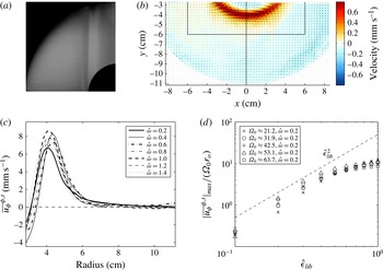
Time-averaged flow field over a period of 5 min for parameters
 $\hat{{\it\omega}}_{lib}=0.4$
,
 $\hat{{\it\epsilon}}_{lib}=0.3$
and
 $E\approx 4\times 10^{-5}$
in the meridional plane using Kalliroscope tracer (a) and in the horizontal plane 4 cm above the equator using PIV tracer (b). The black rectangle and the
 $x=0$
line mark the regions which will be considered in § 4. (c) Shows radial profiles of the averaged azimuthal velocity
 $\overline{u_{{\it\phi}}}^{{\it\phi},t}$
for different
 $\hat{{\it\omega}}_{lib}$
,
 $E\approx 2\times 10^{-5}$
and
 $\hat{{\it\epsilon}}_{lib}=1.0$
. (d) Gives the
 $\hat{{\it\epsilon}}_{lib}$
-dependency of the jet maximum
 $|\overline{u_{{\it\phi}}}^{{\it\phi},t}|_{max}$
, scaled with
 ${\it\Omega}_{0}$
and
 $r_{o}$
, for different
 ${\it\Omega}_{0}$
. The dashed line represents the
 $\hat{{\it\epsilon}}_{lib}^{2}$
-scaling.

Figure 6(a) shows the laser light reflection intensity of the flow in the meridional plane averaged over a period of 5 min for the parameters
 $\hat{{\it\omega}}_{lib}=0.4$
,
 $\hat{{\it\epsilon}}_{lib}=0.3$
and
 $E\approx 4\times 10^{-5}$
. The detached shear layer is represented by the dark layer parallel to the rotation axis. Because the Kalliroscope tracer particles are aligned with the shear flow, they reflect only a small amount of light orthogonal to the meridional laser plane from the jet region. Figure 6(b) shows the corresponding mean velocity field in a horizontal section at height
 $h=4$
cm. The colours show the magnitude of the velocity vectors in
 $\text{mm s}^{-1}$
times the sign of the azimuthal velocity. Therefore, red represents prograde (in direction of rotation) and blue retrograde (opposite direction of rotation) motion. Obviously, in contrast to the classical Stewartson layer with differentially rotating boundaries, the layer here forms a prograde jet, oriented along the tangent cylinder (
 $r\approx 4~\text{cm}$
), where the angular velocity is dropping to zero on both sides beyond the jet region. The maximum velocity of
 $|\boldsymbol{v}|_{max}=0.8~\text{mm s}^{-1}$
is comparatively weak, which is in accordance with the small libration amplitude of
 $\hat{{\it\epsilon}}_{lib}=0.3$
. From figure 6(a), it seems that the Stewartson layer becomes broader with increasing height. This can be confirmed by comparing the PIV fields in three different heights
 $h=(2~\text{cm},4~\text{cm},6~\text{cm})$
and it confirms recent results from an experiment with annular geometry (Klein et al.
Reference Klein, Seelig, Kurgansky, Ghasemi V., Borcia, Will, Schaller, Egbers and Harlander2014; Seelig Reference Seelig2014). The mean flow inside the tangent cylinder is dominated by a weak retrograde flow (compare figure 6
b).
Figure 6(c) shows radial profiles of the averaged azimuthal velocity
 $\overline{u_{{\it\phi}}}^{{\it\phi},t}$
, depending on
 $\hat{{\it\omega}}_{lib}$
, for
 $E\approx 2\times 10^{-5}$
and
 $\hat{{\it\epsilon}}_{lib}=1.0$
. Note that these data are partly in the supercritical regime (figure 1), so that we see some nonlinear effects (e.g. Görtler vortices and Stewartson-layer instabilities). Due to higher
 $\hat{{\it\epsilon}}_{lib}$
, the prograde jet and the retrograde flow inside the tangent cylinder are much stronger than in figure 6(b). It is obvious that the magnitude of the jet and its width depend on the libration frequencies. For the lower libration frequencies (
 $\hat{{\it\omega}}_{lib}=0.2$
), the jet is relatively weak, which can be explained by a higher turbulence grade and the existence of different wave types (trapped waves and spiral waves) and Görtler vortices (Koch et al.
Reference Koch, Harlander, Egbers and Hollerbach2013) that influence the flow dynamics. The strongest jet can be observed at
 $\hat{{\it\omega}}=0.4$
and
 $\hat{{\it\omega}}=1.0$
. By further increasing
 $\hat{{\it\omega}}_{lib}$
, the width of the jet is increasing while its strength is decreasing monotonically due to the less effective excitation (see appendix A). Additionally, the jet shifts closer to the gap centre and the retrograde flow becomes weaker. For high libration frequencies
 $\hat{{\it\omega}}_{lib}>1.6$
(not shown), the jet maximum is drastically reduced by more than 50 % and the retrograde flow contracts or vanishes. Both the prograde jet along and the retrograde flow inside the tangent cylinder are consistent with the experimental findings by Koch et al. (Reference Koch, Harlander, Egbers and Hollerbach2013), Klein et al. (Reference Klein, Seelig, Kurgansky, Ghasemi V., Borcia, Will, Schaller, Egbers and Harlander2014) and Seelig (Reference Seelig2014). Note that the radial profiles for
 $E\approx 4\times 10^{-5}$
, i.e. slower mean rotation (not shown), look similar to figure 6(c) but with about 50 % smaller jet maximum.
Figure 6(d) shows the maximum azimuthal velocity
 $|\overline{u_{{\it\phi}}}^{{\it\phi},t}|_{max}$
of the jet, scaled by
 ${\it\Omega}_{0}\,r_{o}$
, versus the libration amplitude
 $\hat{{\it\epsilon}}_{lib}$
in a logarithmic scale. The measurements have been done at different
 ${\it\Omega}_{0}$
while keeping the libration frequency constant at
 $\hat{{\it\omega}}_{lib}=0.2$
. Obviously, the jet amplitude scales with
 $\hat{{\it\epsilon}}_{lib}^{2}$
(dashed line) for sufficiently small
 $\hat{{\it\epsilon}}_{lib}\leqslant 0.5$
, i.e. when the flow is subcritical. The same scaling could be found numerically by Koch et al. (Reference Koch, Harlander, Egbers and Hollerbach2013) and Sauret & Le Dizès (Reference Sauret and Le Dizès2013) but the latter used libration frequencies larger than
 $2{\it\Omega}_{0}$
to exclude the influences of inertial waves. Note that our setup will not generate an axisymmetric mean flow for frequencies larger than 2, since the excitation librating the inner sphere is too weak. Morize et al. (Reference Morize, Le Bars, Le Gal and Tilgner2010) and Sauret, Le Bars & Le Gal (Reference Sauret, Le Bars and Le Gal2014) also reported such a scaling for tide-driven mean flows, where
 ${\it\epsilon}$
is the deformation strength of the outer boundary. This is not surprising, since librational and tidal forcing share many common features.
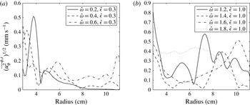
Wave amplitude
 $(\overline{u_{{\it\phi}}^{2}}^{{\it\phi},t})^{1/2}$
for different libration frequencies filtered by a harmonic analysis. The height of measurement is 4 cm above the equator.

Remarkably, when the flow becomes supercritical and Görtler vortices and Stewartson-layer instabilities start to grow, the relative jet amplitude in figure 6(d) decreases and deviates from the
 $\hat{{\it\epsilon}}_{lib}^{2}$
-scaling. This deviation seems to increase with increasing mean rotation
 ${\it\Omega}_{0}$
(compare for instance crosses with squares). That means having a higher turbulence grade, and stronger wave–wave interactions, the jet amplitude is not significantly increasing with increasing
 $\hat{{\it\epsilon}}_{lib}$
. It is not clear whether or not the jet amplitude converges towards a constant value for further increasing
 ${\it\Omega}_{0}$
or
 $\hat{{\it\epsilon}}_{lib}$
, since our apparatus is technically restricted to the used parameters. Moreover, it is also possible that the jet maximum starts to decrease when the flow becomes more and more turbulent.
3.3. Inertial waves in the horizontal plane
In the horizontal plane, we focus on PIV measurements. PIV analyses have been done for some of the parameters shown in figure 4. Figure 7 shows radial profiles of the azimuthally and time-averaged wave amplitude
 $(\overline{u_{{\it\phi}}^{2}}^{{\it\phi},t})^{1/2}$
for different libration frequencies. Using the harmonic analysis, we filtered
 $u_{{\it\theta}}$
such that it contains only the oscillating part of the frequency
 $\hat{{\it\omega}}_{lib}$
. All parameters correspond to the linear inertial wave regime. For the lower frequencies
 $\hat{{\it\omega}}_{lib}\leqslant 0.6$
,
 $\hat{{\it\epsilon}}_{lib}=0.3$
(figure 7
a), the highest wave amplitude is strongly concentrated inside the tangent cylinder (
 $r\leqslant 4~\text{cm}$
). This can be due to stronger axial shear above the librating inner sphere. Figure 7(b) shows the same as figure 7(a) but for higher frequencies
 $\hat{{\it\omega}}=(1.2,1.4,1.6,1.8)$
. To have a more pronounced development, we increased the libration amplitude to
 $\hat{{\it\epsilon}}=1.0$
. Except for
 $\hat{{\it\omega}}=1.8$
, the amplitude maxima are shifted towards the outer boundary, in correspondence with figure 4. The width of the shear layers is increasing with increasing frequency. Note that because of the height
 $h=4~\text{cm}$
, the maxima for the two frequencies
 $\hat{{\it\omega}}=1.6/1.8$
correspond to reflected wave beams coming from the outer boundary. The
 $\hat{{\it\omega}}=1.2$
case looks more complex than the others. Comparing with figure 4, an intersection point of a direct and a reflected wave beam can be seen close to the
 $h=4~\text{cm}$
plane. This strongly affects the wave amplitude.
Horizontal velocity fields for
 $h=2$
cm (a,b) and
 $h=4$
cm (c,d) filtered for the libration frequency with the help of a harmonic analysis. The libration parameters are
 $\hat{{\it\omega}}_{lib}=0.4$
,
 $\hat{{\it\epsilon}}_{lib}=0.3$
and
 $E\approx 4\times 10^{-5}$
; (a,c) show the instantaneous fields for
 $t=t_{0}$
and (b,d) for
 $t=t_{0}+T/4$
. Measurements have been performed in the corotating frame. The colours show the magnitude of the velocity in prograde (red) and retrograde (blue) directions.

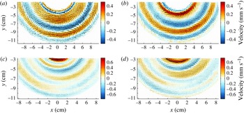
Figure 8 gives an example of a corresponding spatial velocity field measured at two different heights
 $h=2~\text{cm}$
(a,b) and
 $h=4~\text{cm}$
(c,d). It shows four instantaneous fields of the harmonically filtered velocity in the linear regime for parameters
 $\hat{{\it\omega}}_{lib}=0.4$
,
 $\hat{{\it\epsilon}}_{lib}=0.3$
and
 $E\approx 4\times 10^{-5}$
. The colours represent the magnitude of the velocity in
 $\text{mm}~\text{s}^{-1}$
in prograde (red) and retrograde (blue) directions. Obviously, the structures correspond to propagating inertial waves with libration frequency
 $\hat{{\it\omega}}_{lib}=0.4$
. They form nearly perfect circles as expected from the azimuthally symmetric forcing (similar PIV results in Messio et al.
Reference Messio, Morize, Rabaud and Moisy2008; Klein et al.
Reference Klein, Seelig, Kurgansky, Ghasemi V., Borcia, Will, Schaller, Egbers and Harlander2014; Seelig Reference Seelig2014), with small azimuthal asymmetries in the order of
 $10^{-1}~\text{mm s}^{-1}$
. Note that we observed small asymmetries for all analysed libration frequencies in
 $h=4$
cm and
 $h=6$
cm but not in
 $h=2$
cm (see figure 8
a,b). We also observed that even if the directly forced wave shows some asymmetry, the higher harmonics
 $k\hat{{\it\omega}}_{lib}$
,
 $k=2,3,\ldots$
, are usually symmetric. Figure 8(a,c) display the fields at an arbitrary initial time
 $t_{0}$
and figure 8(b,d) at time
 $t_{0}+T/4$
, where
 $T$
is the wave period. From this, the propagation of the inertial waves can be estimated by comparing the left- and right-hand columns of figure 8. After a quarter period, the inertial waves outside the tangent cylinder propagate towards the centre of the sphere and the inertial waves inside the tangent cylinder propagate in the opposite direction, i.e. towards the tangent cylinder. This agrees with the findings from figure 4 for
 $\hat{{\it\omega}}_{lib}=0.4$
, where the phases have opposite signs on the left- and right-hand sides of the Stewartson layer. Note that the maximum velocity at
 $h=4$
cm is about 30 % larger than at
 $h=2~\text{cm}$
. This is due to the velocity peak for
 $r<4~\text{cm}$
, i.e. inside the tangent cylinder (see 3.2), where the inertial oscillations seem to be stronger than in the bulk of the fluid (see also figure 7). In summary, we can say that for all analysed libration amplitudes and frequencies, the wave amplitude is larger inside the tangent cylinder.
4. Nonlinear flow features
4.1. Transition to turbulence for high
 $\hat{{\it\epsilon}}_{lib}$
and small
$\hat{{\it\omega}}_{lib}$


For high libration amplitudes and small libration frequencies, the flow becomes irregular (see e.g. Sauret et al.
Reference Sauret, Cébron, Morize and Le Bars2010, Reference Sauret, Cébron, Le Bars and Le Dizès2012; Koch et al.
Reference Koch, Harlander, Egbers and Hollerbach2013; Sauret et al.
Reference Sauret, Cébron and Le Bars2013). Within this so-called ‘supercritical’ regime (figure 1), instabilities of the Stewartson layer start to grow and nonlinear features arise (e.g. higher harmonics of the inertial waves and the Görtler vortices investigated by Koch et al. (Reference Koch, Harlander, Egbers and Hollerbach2013)). There have been various studies on the transition to the ‘supercritical’ regime for cylindrical geometry (Sauret et al.
Reference Sauret, Cébron, Le Bars and Le Dizès2012; Klein et al.
Reference Klein, Seelig, Kurgansky, Ghasemi V., Borcia, Will, Schaller, Egbers and Harlander2014; Seelig Reference Seelig2014), librating spherical cavities (Sauret et al.
Reference Sauret, Cébron, Morize and Le Bars2010, Reference Sauret, Cébron and Le Bars2013; Sauret & Le Dizès Reference Sauret and Le Dizès2013) and spherical shells (Calkins et al.
Reference Calkins, Noir, Eldredge and Aurnou2010; Koch et al.
Reference Koch, Harlander, Egbers and Hollerbach2013). Note that for
 ${\it\eta}=1/3$
used here, the turbulent regime in the
 $\hat{{\it\omega}}_{lib}$
–
 $\hat{{\it\epsilon}}_{lib}$
parameter space (figure 1) is contracted compared to
 ${\it\eta}=1/2$
, used by Koch et al. (Reference Koch, Harlander, Egbers and Hollerbach2013). This is the reason why we cannot reach a fully developed turbulent flow. Even for the largest possible libration amplitude the flow remains in the so-called Taylor–Görtler regime, where
 $\hat{{\it\epsilon}}_{lib}$
is larger than a critical value but not large enough for full turbulence (Sauret et al.
Reference Sauret, Cébron, Le Bars and Le Dizès2012, Reference Sauret, Cébron and Le Bars2013). However, our goal is to investigate flow patterns in the weakly turbulent flow with the help of PIV. In this regime, nonlinear interactions are present in addition to the forced inertial waves.
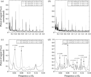
Power spectra taken from a Fourier analysis, (a,b) averaged over the
 $x=0$
line for three different velocity field time series with libration frequencies
 $\hat{{\it\omega}}_{lib}=(0.2,0.4,0.6)$
by solid, dashed and dotted lines, respectively, and (c,d) averaged over the inner region (
 $y\leqslant 6$
cm) in dashed and the outer region (
 $y>6$
cm) in solid lines. The libration amplitude was
 $\hat{{\it\epsilon}}_{lib}=1.0$
for each frequency.

We start by giving an overview of dominant frequencies in the ‘supercritical’ regime using PIV data. A Fourier analysis of the azimuthal velocity has been done for each grid point along the
 $x=0$
line marked in figure 6(b). These spectra were averaged to obtain a mean spectrum. Mean power spectra are shown in figure 9(a,b) for three different velocity time series in the corotating frame with libration frequencies
 $\hat{{\it\omega}}_{lib}=(0.2,0.4,0.6)$
in solid, dashed and dotted lines, respectively. Figure 9(a) shows the spectra for
 $E\approx 4\times 10^{-5}$
(
 ${\it\Omega}_{0}\approx 24.4~\text{r.p.m.}$
) and figure 9(b) for
 $E\approx 2\times 10^{-5}$
(
 ${\it\Omega}_{0}\approx 47.8~\text{r.p.m.}$
). The libration amplitude was
 $\hat{{\it\epsilon}}_{lib}=1.0$
for each frequency. At this point, we remind the reader that
 $\hat{{\it\omega}}_{lib}$
refers to the libration frequency and
 $\hat{{\it\omega}}$
refers to particular wave frequencies that stand out in figure 9(a–d). It is obvious that the highest peaks agree with their respective libration frequencies in both cases (a) and (b). For each frequency at least two higher harmonics
 $\hat{{\it\omega}}=k\,\hat{{\it\omega}}_{lib}$
,
 $k=2,3$
, in the range
 $\hat{{\it\omega}}\leqslant 2$
can be detected as monotonically decreasing peaks in the spectra (figure 9
a,b). Higher harmonics are nonlinear features and have numerically and experimentally been discussed in Koch et al. (Reference Koch, Harlander, Egbers and Hollerbach2013). Due to the smaller Ekman number, the dissipation in (b) is smaller than in (a), which gives stronger signals. However, the main difference between the two cases lies in the low-frequency range
 $\hat{{\it\omega}}<0.2$
. To highlight these differences, we magnified the low-frequency range
 $0\leqslant \hat{{\it\omega}}\leqslant 0.2$
of figure 9(a,b) and show it in figure 9(c,d). The averaging is divided into a part
 $y\leqslant 6$
cm (dashed line), representing the region around the tangent cylinder, and a part
 $y>6$
cm (solid line), representing the region outside the tangent cylinder. The labelled frequencies will be employed later for figures 11 and 12. Due to a higher grade of turbulence for
 ${\it\Omega}_{0}=47.8~\text{r.p.m.}$
(figure 9
d), the fluctuations and also the spectral peaks are significantly higher in this frequency band. Surprisingly, some signals exceed even the directly forced frequencies, e.g. the peak close to
 $\hat{{\it\omega}}\approx 0.08$
, which exceeds the inertial wave signal for
 $\hat{{\it\omega}}=0.2$
in figure 9(b). Remarkably, this peak becomes less dominant in the outer region
 $y>6$
cm (solid line in figure 9
c,d). Therefore, the corresponding spatial structure must be concentrated close to the Stewartson layer (detailed discussion in § 4.2). Further, the frequency of this peak depends only weakly on the libration parameters
 $\hat{{\it\omega}}_{lib}$
and
 $\hat{{\it\epsilon}}_{lib}$
as well as the mean rotation
 ${\it\Omega}_{0}$
. This result is consistent with findings from Zimmerman, Triana & Lathrop (Reference Zimmerman, Triana and Lathrop2011) and Rieutord et al. (Reference Rieutord, Triana, Zimmerman and Lathrop2012), who studied the flow in a large 3 m spherical shell with a similar aspect ratio as our shell. They detected a low-frequency phenomenon which seems to be independent of the Rossby number
 $Ro_{d}$
. However, the underlying mechanism remains unclear.
In addition to the peak at
 $\hat{{\it\omega}}\approx 0.08$
, other noticeable peaks can be found in the low-frequency range
 $\hat{{\it\omega}}<0.2$
(labelled in figure 9
c,d), whose corresponding spatial structure will be discussed in § 4.2. Hollerbach (Reference Hollerbach2003), Schaeffer & Cardin (Reference Schaeffer and Cardin2005a
,Reference Schaeffer and Cardin
b
) and Wicht (Reference Wicht2014) explained all the low-frequency features as Rossby modes or Rossby-wave instabilities of the Stewartson layer. Their amplitude, wavenumber and spatial structure depend on the geometry, the rotation rate and also on the sign of
 $Ro_{d}$
. Particularly, the sign of
 $Ro_{d}$
plays a crucial role in spherical shells. For libration,
 $Ro_{d}$
varies between negative and positive values. It is therefore likely that typical structures related to both positive and negative
 $Ro_{d}$
can be found in our experiments with inner sphere libration. In the following, we will discuss the horizontal structure of dominant low-frequency modes and compare those with numerical results reported by e.g. Hollerbach (Reference Hollerbach2003), Schaeffer & Cardin (Reference Schaeffer and Cardin2005a
,Reference Schaeffer and Cardin
b
) and Wicht (Reference Wicht2014).
4.2. Instability of the Stewartson layer – Rossby-wave instability
As discussed in § 3.2, inner sphere libration gives rise to a prograde Stewartson layer depending on the libration parameters
 $\hat{{\it\omega}}_{lib}$
and
 $\hat{{\it\epsilon}}_{lib}$
(Koch et al.
Reference Koch, Harlander, Egbers and Hollerbach2013; Sauret & Le Dizès Reference Sauret and Le Dizès2013). Similar to differential rotation, this layer becomes unstable for a critical shear, i.e. when the libration amplitude exceeds a certain threshold (figure 1). Schaeffer & Cardin (Reference Schaeffer and Cardin2005a
) considered a quasigeostrophic model for a spherical cavity with differentially rotating polar caps with radius
 $r_{0}=0.35$
. They found that in case of super-rotation (
 $Ro_{d}>0$
), the instabilities develop in the form of spirals (hereafter referred to as ‘spiral waves’) essentially located outside the tangent cylinder. In case of subrotation (
 $Ro_{d}<0$
), the instability is trapped near
 $r_{0}$
and seems to be localised inside the tangent cylinder (hereafter referred to as ‘trapped waves’). In both cases, the instabilities drift in the prograde direction. To explain the nature of these instabilities, they introduced the
 ${\it\beta}$
-effect depending on the fluid depth within the spherical container. They found that instabilities occur for Rossby numbers larger than a critical value
 $Ro_{d}>Ro_{d,crit}$
, where the critical Rossby number scales as
 $Ro_{d,crit}\sim {\it\beta}E^{1/2}$
(in contrast to flat containers, where
 $Ro_{d,crit}\sim E^{3/4}$
). The
 ${\it\beta}$
parameter is defined as
 $$\begin{eqnarray}{\it\beta}=\frac{1}{L}\frac{\text{d}L}{\text{d}r},\end{eqnarray}$$
where
 $L(r)$
is the half-height of the full sphere measured parallel to the axis of rotation. With increasing radius, the height decreases and therefore
 ${\it\beta}<0$
for all
 $r$
. Schaeffer & Cardin (Reference Schaeffer and Cardin2005a
) argued that the spiral waves in the super-rotational case occur due this property of
 ${\it\beta}$
in accordance with decreasing
 $Ro_{d,crit}$
.
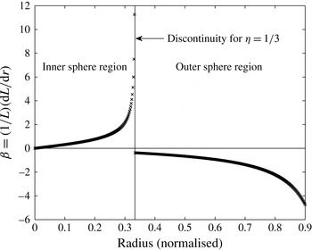
 ${\it\beta}$
parameter as a function of radius in a spherical shell. A discontinuity for
 ${\it\beta}$
at
 $r_{i}$
occurs due to abrupt change in fluid depth.

Velocity fields in the horizontal plane at 4 cm above the equator for
 $\hat{{\it\omega}}_{lib}=0.2$
,
 $\hat{{\it\epsilon}}_{lib}=1.0$
,
 ${\it\Omega}_{0}\approx 24.4~\text{r.p.m.}$
and
 $E\approx 4\times 10^{-5}$
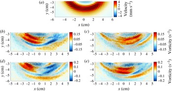
. All fields are magnified as indicated by the black box in figure 6(b). (a) Shows the mean flow; (b–e) show filtered velocities for the frequencies marked in figure 9(c). Colours in (a) show the magnitude of velocity (red – prograde, blue – retrograde) and in (b–e) the relative vorticity.

Figure 10 shows the
 ${\it\beta}$
parameter as a function of radius (4.1) for the present spherical shell with
 ${\it\eta}=1/3$
. The vertical line marks the discontinuity at
 ${\it\eta}=1/3$
where the tangent cylinder touches the inner sphere’s equator. Obviously,
 ${\it\beta}$
is not a continuous function of radius
 $r$
. The function is subdivided into a part inside the tangent cylinder with
 $r<r_{i}$
where
 ${\it\beta}>0$
, and a part outside with
 $r\geqslant r_{i}$
where
 ${\it\beta}<0$
. The outer part is identical to the full sphere. For
 $r\rightarrow r_{i}$
from the inner region,
 ${\it\beta}$
tends to infinity due to the height jump at
 $r_{i}$
. Such height jumps were found to have a significant influence on the flow (Hide & Titman Reference Hide and Titman1967; Hollerbach Reference Hollerbach2003; Schaeffer & Cardin Reference Schaeffer and Cardin2005a
; Aguiar & Read Reference Aguiar and Read2006). Due to the opposite signs of
 ${\it\beta}$
inside and outside the tangent cylinder, Schaeffer & Cardin (Reference Schaeffer and Cardin2005a
) suggested that the instabilities travel in opposite directions inside and outside the tangent cylinder. They further assumed that for
 $Ro_{d}>0$
the instabilities trigger prograde-propagating modes outside the tangent cylinder where
 $|{\it\beta}|$
is small. In contrast, inside the tangent cylinder the instability threshold (
 $Ro_{d,crit}\sim {\it\beta}E^{1/2}$
) is much higher and the instability seems to be of different nature (Hollerbach Reference Hollerbach2003).
While Schaeffer & Cardin (Reference Schaeffer and Cardin2005a
) used only differentially rotating polar caps in a full sphere, the differentially rotating spherical shell was analysed numerically by Hollerbach (Reference Hollerbach2003) and, most recently, by Wicht (Reference Wicht2014). Both authors found strong differences between positive and negative
 $Ro_{d}$
. For
 $Ro_{d}>0$
, the instabilities look similar to the spiral waves of a full sphere (Schaeffer & Cardin Reference Schaeffer and Cardin2005a
). The case
 $Ro_{d}<0$
shows an instability with azimuthal wavenumber
 $m=1$
for a large range of Ekman numbers (Hollerbach Reference Hollerbach2003). Wicht (Reference Wicht2014) found that these so-called Rossby modes exhibit a nearly geostrophic (barotropic) structure, i.e. columnar patterns parallel to the axis of rotation with a weak
 $z$
-dependence. Hence, the conservation of potential vorticity can approximately be used to explain the instability qualitatively (Hollerbach Reference Hollerbach2003; Schaeffer & Cardin Reference Schaeffer and Cardin2005a
). The potential vorticity is defined as
 $$\begin{eqnarray}PV=\frac{2+Ro_{d}(\boldsymbol{{\rm\nabla}}\times \boldsymbol{U}_{0})_{z}}{L(r)},\end{eqnarray}$$
where
 $\boldsymbol{U}_{0}$
is the basic state velocity. From this, it can be derived that for positive differential rotation
 $(Ro_{d}>0)$
a prograde Stewartson shear layer with negative absolute vorticity is produced. In that case, perturbations can be amplified while moving away from the Stewartson layer into shallower regions. Therefore, perturbations can be amplified inside and outside the tangent cylinder but, due to smaller
 ${\it\beta}$
, Schaeffer & Cardin (Reference Schaeffer and Cardin2005a
) argued that the perturbations will mainly develop outside the tangent cylinder. In contrast, for
 $Ro_{d}<0$
all perturbations moving away from the Stewartson layer should be damped. Therefore, the origin of the instability for
 $Ro_{d}<0$
in a spherical shell remains unclear. Hollerbach (Reference Hollerbach2003) argued that the discontinuity in potential vorticity at
 $r=r_{i}$
is responsible for the evolution of trapped waves. This argument fits meteorological observations that forced Rossby waves are traveling along a zonally aligned jet stream containing a discontinuity in potential vorticity (e.g. Schwierz, Dirren & Davies Reference Schwierz, Dirren and Davies2004).
Next we focus on the present experiment with a librating inner sphere, where
 $Ro_{d}$
shows a periodic variation in time (2.1). In this case we expect that the typical instability patterns for positive and negative
 $Ro_{d}$
will occur. If not otherwise indicated, all the following results correspond with
 $Ro_{lib}=\hat{{\it\epsilon}}_{lib}=1.0$
. Figure 11(a) shows an averaged flow field at
 $h=4$
cm for the parameters
 $\hat{{\it\omega}}_{lib}=0.2$
,
 $\hat{{\it\epsilon}}_{lib}=1.0$
,
 ${\it\Omega}_{0}\approx 24.4~\text{r.p.m.}$
and
 $E\approx 4\times 10^{-5}$
for the region within the black box highlighted in figure 6(b). The jet aligned with the tangent cylinder is always prograde for a librating inner sphere (Koch et al.
Reference Koch, Harlander, Egbers and Hollerbach2013), implying an amplification of perturbations moving away from the tangent cylinder into shallower regions (Schaeffer & Cardin Reference Schaeffer and Cardin2005a
).
Figure 11(b–e) show the corresponding velocity fields. The data have been filtered using a harmonic analysis for
 $\hat{{\it\omega}}=0.079$
(b,c) and
 $\hat{{\it\omega}}=0.043$
(d,e), the two prominent peaks in the low-frequency range of figure 9(c). The colours represent the relative vorticity. The figures show instantaneous fields at time
 $t_{0}$
(b,d) and after a quarter period at
 $t_{0}+T/4$
(c,e). It is obvious that both patterns correspond to wave trains that are trapped within the Stewartson layer and are propagating retrograde (hereafter referred to as ‘trapped Rossby waves’). These patterns resemble the modes found e.g. in Schaeffer & Cardin (Reference Schaeffer and Cardin2005b
) for
 $Ro_{d}<0$
and Schwierz et al. (Reference Schwierz, Dirren and Davies2004). The retrograde drift agrees with the assumption of Schaeffer & Cardin (Reference Schaeffer and Cardin2005a
) that, due to the positive
 ${\it\beta}$
parameter inside the tangent cylinder of a spherical shell, perturbations are propagating against the mean rotation. It thus seems natural that the trapped Rossby waves in figure 11 are related to the retrograde phase of the libration cycle. Further, these wave trains can be found at all heights
 $h=(2~\text{cm},4~\text{cm},6~\text{cm})$
, which infers a columnar structure with weak
 $z$
dependence (Wicht Reference Wicht2014).
In contrast to Hollerbach (Reference Hollerbach2003), who numerically found mainly instabilities with azimuthal wavenumber
 $m=1$
, we observed higher wavenumbers
 $m=2$
(b,c) and
 $m=3$
(d,e). Our findings further imply that with decreasing frequency the azimuthal wavenumber
 $m$
increases and the phase velocity decreases, which is typical for Rossby waves (Pedlosky Reference Pedlosky1987). It remains somewhat puzzling why the azimuthal wavenumber is higher as for steady differential rotation studied by Hollerbach (Reference Hollerbach2003). However, in contrast to Hollerbach’s study, the jet here is prograde, and we further observe a weaker retrograde mean flow inside the tangent cylinder that might also affect the wavenumber of the trapped Rossby waves.
Appearance, amplitude and frequency of the trapped Rossby waves depending on the libration frequency. The libration amplitude is
 $\hat{{\it\epsilon}}_{lib}=1.0$
. The abbreviations mean:
 $\text{cs}/\text{ws}$
–
 $\text{clear}/\text{weak}$
signal in power spectrum,
 $\text{cv}/\text{wv}$
–
 $\text{clear}/\text{weak}$
vortices (waves),
 $\text{sv}$
– structural vacillations and * means wave detection in all measured heights
 $h=(2,4,6)$
cm, which indicates columnar patterns.
 $|Y({\it\omega})|_{rel}$
is the signal power of the respective frequency normalised by the maximum signal power of the trapped Rossby-wave modes.

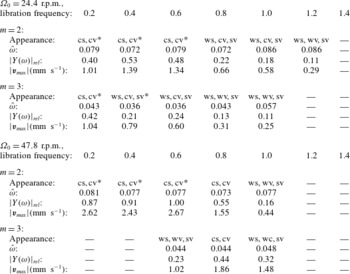
Table 2 summarises the occurrence of the trapped Rossby waves in our experiment. Note that the
 $m=3$
trapped Rossby wave could not be detected for low libration frequencies in the data for
 ${\it\Omega}_{0}\approx 47.8~\text{r.p.m.}$
, since the flow is too turbulent for a clear wave development. When the turbulence grade decreases with increasing libration frequency (
 $0.6\leqslant \hat{{\it\omega}}_{lib}\leqslant 1.0$
), the
 $m=3$
wave could be detected as a clear peak in the power spectrum (not shown). For
 $\hat{{\it\omega}}_{lib}\geqslant 1.2$
, the libration efficiency is too weak to excite trapped Rossby waves (appendix A).
Velocity fields in the horizontal plane at 4 cm above the equator for
 $\hat{{\it\omega}}_{lib}=0.2$
,
 $\hat{{\it\epsilon}}_{lib}=1.0$
,
 ${\it\Omega}_{0}\approx 47.8~\text{r.p.m.}$
and
 $E\approx 2\times 10^{-5}$
. Shown are the filtered velocities for the frequencies (from (a) to (f):
 $\hat{{\it\omega}}=(0.038,0.064,0.110,0.131,0.155,0.169)$
) marked in figure 9(d). The colours show the magnitude of velocity (red – prograde, blue – retrograde).

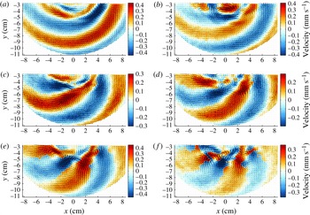
Next we discuss flow features that are not trapped within the Stewartson layer. These structures are related to the
 $Ro_{d}>0$
case and are also part of the low-frequency band
 $\hat{{\it\omega}}<0.2$
(figure 9
d) in the ‘supercritical’ regime. Figure 12(a–f) show velocity fields in the horizontal plane at height
 $h=4~\text{cm}$
for
 $\hat{{\it\omega}}_{lib}=0.2$
,
 $\hat{{\it\epsilon}}_{lib}=1.0$
,
 ${\it\Omega}_{0}\approx 47.8~\text{r.p.m.}$
and
 $E\approx 2\times 10^{-5}$
, i.e. the same parameters as before but with a smaller Ekman number. The data have been filtered with a harmonic analysis for the respective frequencies given in the caption. The frequencies have been chosen from figure 9(d) corresponding to further prominent peaks in the low-frequency range
 $\hat{{\it\omega}}<0.2$
. But note that the peak height is not that remarkable as for the trapped Rossby waves. The colours show the magnitude of the velocity in
 $\text{mm s}^{-1}$
, where red corresponds to a prograde and blue to a retrograde motion. Obviously, the waves presented here differ from the trapped Rossby waves shown in figure 11. They show spiral structures filling the entire gap outside the tangent cylinder while the velocity inside is comparatively weak (hereafter referred to as ‘spiral waves’). Within the spiral waves, vortices are embedded (e.g. in figure 12
e,f). In contrast to the trapped Rossby waves, these vortices are located at the outer edge of the Stewartson layer. The phase velocity of the spiral waves (not shown) exhibits a prograde drift for all frequencies in figure 12. These properties of the spiral waves resemble the spiral Rossby waves found in Schaeffer & Cardin (Reference Schaeffer and Cardin2005a
) for positive
 $Ro_{d}$
. It is thus obvious to assume that the excitation of spiral waves is related to the prograde phase of the libration cycle. The maximum velocity of each spiral wave in figure 12 is about six times smaller than for the trapped
 $m=2$
Rossby wave for the same parameters (see table 2). Hence, the trapped Rossby waves are more distinct than the spiral waves and have a stronger influence on the flow for both analysed Ekman numbers (compare figure 9
c,d). Similar to the trapped Rossby waves, the spiral waves become weaker when the libration frequency is increasing since then the flow becomes ‘subcritical’ (see figure 1).
Regarding the azimuthal wavenumber
 $m$
of the spiral waves (figure 12), it seems that, in contrast to the trapped waves,
 $m$
is increasing with increasing frequency. Further, the radial wavenumber is decreasing with increasing frequency. This behaviour does not change when we go to the slower rotation rate
 ${\it\Omega}_{0}\approx 24.4~\text{r.p.m.}$
; however, the spiral waves become less prominent. The azimuthal wavenumber of the spiral waves is usually larger than that of the trapped waves, in agreement with findings by Hollerbach (Reference Hollerbach2003) comparing the
 $Ro_{d}>0$
with the
 $Ro_{d}<0$
case. For the slower rotation rate
 ${\it\Omega}_{0}\approx 24.4~\text{r.p.m.}$
, the total azimuthal wavenumber of the spiral waves becomes smaller (not shown), which is also in agreement with the findings by Hollerbach (Reference Hollerbach2003).
5. Conclusion and future work
We experimentally studied linear and nonlinear inertial waves in a spherical shell. The shell rotated with a mean angular velocity
 ${\it\Omega}_{0}$
. Further, an additional oscillation, called longitudinal libration, was applied for the inner sphere. First, we used inner sphere libration to excite inertial waves with a defined frequency in the range
 $0\leqslant \hat{{\it\omega}}\leqslant 2$
. Second, we studied Stewartson layers that occurred for the spherical shell in the form of a cylinder tangential to the inner sphere’s equator. For sufficiently high/low libration amplitudes/frequencies, the Stewartson layer became unstable. Consequently, waves slowly drifting in pro- and retrograde directions and with different azimuthal and radial wavenumbers have been excited.
The Stewartson layer, excited by inner sphere libration (Koch et al.
Reference Koch, Harlander, Egbers and Hollerbach2013; Sauret & Le Dizès Reference Sauret and Le Dizès2013), consisted of a prograde jet aligned with the tangent cylinder, i.e. at
 $r=r_{i}$
, that became wider with increasing height. This jet was found to have the maximum velocity for libration frequencies around
 $\hat{{\it\omega}}_{lib}=0.4$
to
 $\hat{{\it\omega}}_{lib}=0.6$
and became weaker for further increasing
 $\hat{{\it\omega}}_{lib}$
because the libration efficiency decreased. This corresponds to what we have found for the inertial wave amplitudes. Further, we found that the jet amplitude scales with
 $\hat{{\it\epsilon}}_{lib}^{2}$
when the libration amplitude is sufficiently small, i.e. the flow is subcritical (Morize et al.
Reference Morize, Le Bars, Le Gal and Tilgner2010; Koch et al.
Reference Koch, Harlander, Egbers and Hollerbach2013; Sauret & Le Dizès Reference Sauret and Le Dizès2013; Sauret et al.
Reference Sauret, Le Bars and Le Gal2014). In the supercritical regime, where several instabilities occurred, the jet amplitude deviated from the
 $\hat{{\it\epsilon}}_{lib}^{2}$
-scaling. The reason might be a stronger wave–wave interaction in a higher turbulence grade, which seemed to suppress a strong amplification of the axisymmetric mean flow for increasing libration amplitudes.
Due to libration, linear inertial waves have been excited at the critical latitude and the wave energy then propagates in directions tangential to the inner sphere. We studied these waves and found that for small
 $\hat{{\it\epsilon}}_{lib}$
the Stewartson layer is stable and inertial waves are zonally symmetric. The group velocity of plane inertial waves points north- and southward along inclined characteristics. In spite of the present mean zonal flow, we found that the inertial wave shear layers are approximately straight lines, in accordance to findings e.g. by Tilgner (Reference Tilgner1999), Harlander & Maas (Reference Harlander and Maas2006) or Borcia & Harlander (Reference Borcia and Harlander2013).
The reflection behaviour of the inertial waves at inclined boundaries was in good agreement with the 2D ray-tracing model. We analysed different frequencies for which attractors occur. But it should be mentioned that in general a larger inner sphere would be more appropriate to detect simple attractors, since then the excitation is stronger and attractor windows are wider.
For all analysed libration frequencies, the wave amplitude was found to be highest above the inner sphere. This can be explained by a stronger wave forcing due to a stronger axial shear in the region above the librating inner sphere, i.e. inside the tangent cylinder (Rieutord et al. Reference Rieutord, Triana, Zimmerman and Lathrop2012).
When the libration amplitude exceeded a certain threshold (figure 1), the Stewartson layer became unstable. Due to fluid-depth variations in the spherical cavity, instabilities radiating away from the Stewartson layer can be amplified in both directions (Schaeffer & Cardin Reference Schaeffer and Cardin2005a
). Within this ‘supercritical regime’, we found prominent low-frequency patterns that correspond to slowly drifting waves. The frequency of these waves was found to be nearly independent of the libration parameters. Further, peaks in the power spectra of velocity time series for frequencies
 $\hat{{\it\omega}}<0.2$
became remarkably higher for smaller Ekman numbers. Most of the peaks correspond to two types of slowly drifting waves, trapped waves and spiral waves. We suggest that inner sphere libration is responsible for the excitation of the different wave types usually assigned to positive and negative
 $Ro_{d}$
, since for libration the Rossby number varies between
 $-1\leqslant Ro_{d}(t)\leqslant 1$
.
One of the detected wave types showed a retrograde drift and was trapped within the Stewartson layer. For these trapped Rossby waves, we found azimuthal wavenumbers of
 $m=2$
and
 $m=3$
(see table 2). The appearance and the power of these waves were strongly dependent on the libration parameters. Note that for high
 $\hat{{\it\epsilon}}_{lib}$
and low
 $\hat{{\it\omega}}_{lib}$
we could not detect a clear trapped wave development at smaller Ekman numbers, particularly for the
 $m=3$
wave, due to a higher turbulence grade. Here, spiral waves became more prominent, which caused a strong wave–wave interaction. These interactions seemed to suppress the
 $m=3$
wave. Nevertheless, the total azimuthal wavenumber was not influenced by changing the Ekman number.
The measurements showed that the trapped waves form columnar patterns with a weak axial variation (Wicht Reference Wicht2014). In agreement with results from Hollerbach (Reference Hollerbach2003), Schaeffer & Cardin (Reference Schaeffer and Cardin2005a
,Reference Schaeffer and Cardin
b
) or Wicht (Reference Wicht2014), we associate these waves with columnar slowly drifting Rossby modes. Schaeffer & Cardin (Reference Schaeffer and Cardin2005a
) found similar waves for negative differential rotation (
 $Ro_{d}<0$
). This implies that the detected trapped waves are connected to the retrograde phase of the libration cycle. The trapping results from a discontinuity in potential vorticity due to a sudden change of fluid depth in the region of the Stewartson layer (Hollerbach Reference Hollerbach2003).
The second wave type showed a prograde drift and had a spiral shape that filled the whole gap outside the Stewartson layer. The spiral waves are connected to the prograde phase of the libration cycle. Schaeffer & Cardin (Reference Schaeffer and Cardin2005a
) described those waves for positive differential rotation (
 $Ro_{d}>0$
). They became prominent for small Ekman numbers, i.e. high rotation rates, and were associated with an increasing turbulence grade. Further, they revealed a wide variety of radial and azimuthal wavenumbers in the low-frequency band
 $\hat{{\it\omega}}<0.2$
. For very low frequencies
 $\hat{{\it\omega}}<0.05$
, the azimuthal wavenumber tended to zero but the radial wavenumber was increasing. In this regime, the patterns can be seen as variations of the mean flow. When the wave frequency was increasing, the azimuthal wavenumber and the phase speed were increasing, too. In contrast to the trapped waves, the azimuthal wavenumber of the spiral waves was also increasing for smaller Ekman numbers, i.e. faster rotation rates
 ${\it\Omega}_{0}$
, which is in agreement with numerical findings by Hollerbach (Reference Hollerbach2003). Further, we usually found the azimuthal wavenumber of the spiral Rossby waves to be higher than that of the trapped waves. The reason for this difference must be the abrupt change in fluid depth in a spherical gap, as was discussed by Hollerbach (Reference Hollerbach2003) and Schaeffer & Cardin (Reference Schaeffer and Cardin2005a
).
We further found hints for triads due to parametric subharmonic instability. This is a resonant wave–wave interaction where a primary wave becomes unstable due to infinitesimal perturbations, transferring energy to two secondary waves with smaller scales (Bourget et al.
Reference Bourget, Dauxois, Joubaud and Odier2013). These so-called resonant triads must satisfy the conditions
 $|{\it\omega}_{0}|=|{\it\omega}_{1}|\pm |{\it\omega}_{2}|$
,
 $m_{0}=m_{2}-m_{1}$
and
 $n_{0}=n_{2}-n_{1}$
, where
 $m$
and
 $n$
are the azimuthal and axial wavenumbers (Bordes et al.
Reference Bordes, Moisy, Dauxois and Cortet2012). We found a possible triad of inertial waves in our data for the forced frequency
 $|\hat{{\it\omega}}_{lib}|\approx 0.8$
and two secondary peaks in the power spectrum for
 $|\hat{{\it\omega}}|\approx 0.2$
and
 $|\hat{{\it\omega}}|\approx 0.6$
. Note that the forced wave is close to the attractor frequency
 $\hat{{\it\omega}}=0.82\pm 0.01$
, i.e. the diamond-shaped attractor studied by Koch et al. (Reference Koch, Harlander, Egbers and Hollerbach2013), which obviously intensified the instability. In figure 9(a,b), there are two remarkable peaks at
 $|\hat{{\it\omega}}_{lib}|=0.6\pm 0.079$
around the forcing frequency. Both peaks match the frequency of the trapped Rossby wave at
 $|\hat{{\it\omega}}|=0.079$
. Therefore, there might also be a coupling between forced inertial waves and low-frequency Rossby waves. Further analyses, particularly of the corresponding wavenumbers, are necessary to confirm the existence of the parametric subharmonic instability but this is beyond the scope of the present work.
Finally, we should mention that we also sampled some data for differential rotation. In case of super-rotation (
 $Ro_{d}>0$
), the detected patterns are spiral waves with a wide range of wavenumbers similar to the results obtained from inner sphere libration. As expected from libration, most of the spirals arising from positive differential rotation appeared in the low-frequency band
 $\hat{{\it\omega}}<0.2$
. For negative
 $Ro_{d}$
, we were able to detect a retrograde drifting
 $m=1$
Rossby mode which was dominant over a wide range of
 $Ro_{d}$
(Hollerbach Reference Hollerbach2003; Rieutord et al.
Reference Rieutord, Triana, Zimmerman and Lathrop2012; Wicht Reference Wicht2014), while its frequency was nearly constant at about
 $\hat{{\it\omega}}=0.09\pm 0.01$
. Its horizontal structure resembles the trapped waves found for inner sphere libration. In the counter-rotation range
 $-2.5\leqslant Ro_{d}\leqslant -1.0$
, we detected dominant inertial modes that have previously been discussed by Triana (Reference Triana2011) and Rieutord et al. (Reference Rieutord, Triana, Zimmerman and Lathrop2012). However, a detailed discussion of these data is beyond the scope of the present paper and will follow in a future work.
Acknowledgements
M.H. was financed by the DLR (grant no. 50 WM 0822) and is now supported by the DFG (grant no. HA 2932/7-1). M.H. and U.H. thank S. Triana and T. Seelig for many fruitful discussions. We further thank S. Jahangir for carrying out a lot of the experiments. A special thanks goes to S. Dahley for setting up the experimental apparatus that was originally funded by the DFG grant no. EG 100/1 to C.E. We also thank the anonymous reviewers for their critical remarks that helped to improve the quality of the final version.
Supplementary material
Supplementary material is available at http://dx.doi.org/10.1017/jfm.2015.743.
Appendix A
We present how the excursion of the inner sphere is related to its radius and the libration parameters
 $\hat{{\it\omega}}_{lib}$
and
 $\hat{{\it\epsilon}}_{lib}$
. We recall that the libration of the inner sphere in the rotating frame of reference reads
 $$\begin{eqnarray}{\it\Omega}_{i}(t)^{\prime }=\hat{{\it\epsilon}}_{lib}{\it\Omega}_{0}\cos (\hat{{\it\omega}}_{lib}{\it\Omega}_{0}t),\end{eqnarray}$$
where the prime denotes only the oscillating part. Then, the tangential velocity
 $v_{T}$
of the oscillating inner sphere is given by
 $$\begin{eqnarray}v_{T}=\frac{\text{d}s}{\text{d}t}=|{\it\bf\Omega}_{i}(t)^{\prime }\times \boldsymbol{r}|={\it\Omega}_{i}(t)^{\prime }r\sin {\it\alpha},\end{eqnarray}$$
where
 ${\it\alpha}=90^{\circ }-{\it\vartheta}_{c}$
is the angle between the radius and the rotation axis and
 ${\it\vartheta}_{c}$
the ‘critical’ point on the inner sphere where inertial waves will be excited. The excursion of the inner sphere is represented by
 $s$
. Inserting (A 1) into (A 2) and integrating gives an equation for the excursion
 $s$
of the inner sphere:
 $$\begin{eqnarray}s(t)=\frac{\hat{{\it\epsilon}}_{lib}}{\hat{{\it\omega}}_{lib}}r\sin {\it\alpha}\sin (\hat{{\it\omega}}_{lib}{\it\Omega}_{0}t).\end{eqnarray}$$
The amplitude of the excursion
 $s_{max}$
is then
 $$\begin{eqnarray}s_{max}=\frac{\hat{{\it\epsilon}}_{lib}}{\hat{{\it\omega}}_{lib}}r_{\bot },\quad r_{\bot }=r\sin {\it\alpha}.\end{eqnarray}$$
From this simple expression, it can be seen that the excursion does not depend on the mean rotation rate
 ${\it\Omega}_{0}$
. Here,
 $r_{\bot }$
is the effective radius orthogonal to the rotation axis. When the ‘critical’ point
 ${\it\vartheta}_{c}$
is moving towards the pole of the inner sphere (increasing inertial wave frequency),
 ${\it\alpha}$
tends to zero and thus
 $r_{\bot }$
becomes small. The excursion amplitude
 $s_{max}$
of the inner sphere at this point
 ${\it\vartheta}_{c}$
, where inertial waves are excited, is therefore also decreasing and the forcing becomes weaker. Further, it can be seen that the inner sphere excursion, and therefore the forcing, becomes weaker when the libration frequency is increased while keeping the libration amplitude constant.