4.1. Influence of topography and tidal frequency to viscous dissipation

We first examine the flow structure and distribution of viscous dissipation when the tidal effect is sufficiently strong. Figure 3 presents the temporally averaged velocity vectors (left half) and viscous dissipation field in log scale (right half) of different topographies with $\omega =0.04$. The normalized height of topography $h/H$ corresponds to $0$, $0.25$, $0.5$ and $0.75$ in figure 3(a–d). For $h/H=0$, we observe a large-scale circulation that downwells underneath the cold plate and upwells gradually during the horizontal movement towards the hot plate. Such mean flow structure is consistent with previous observations in horizontal convection without a tidal force (Hughes & Griffiths Reference Hughes and Griffiths2008; Shishkina Reference Shishkina2017). As shown in figure 3(a), the flow strength underneath the hot plate is weak. When topography is introduced, strong flow can be observed in the area adjacent to the topography. As shown in figure 3(c,d), for $h/H=0.5$ and $h/H=0.75$, such strong flow near topography develops vortices that change the single-roll large-scale circulation into a multi-roll structure. Quantitatively similar flow structures (e.g. vortical flows in the vicinity of topography) and distribution of $\epsilon _v$ can be found in figure 3(e), which corresponds to the three-dimensional simulation with similar conditions as figure 3(c). Owing to the formation of the larger vortex near the topography, the local viscous dissipation $\epsilon _v$ is significantly enhanced. Such dissipation enhancement near topography agrees with field observations in the ocean interior. Previous field studies explain this enhancement as a result of the breaking of internal waves generated by a tide–topography interaction (Waterhouse et al. Reference Waterhouse2014). The angle of the internal wave is determined by the buoyancy frequency $N\equiv \sqrt {\alpha g({\partial \theta }/{\partial z}})$ and tidal frequency according to the dispersion relation (Kundu et al. Reference Kundu, Cohen and Dowling2016):

(4.1)\begin{equation} \tan\beta=\sqrt{\frac{\omega^2}{N_*^2-\omega^2}}, \end{equation}

where $\beta$ is the angle between the group velocity and the horizontal direction, and $N_*\equiv N/(1/t_{ref})$ is the dimensionless buoyancy frequency. The existence of internal waves requires $N_*/\omega >1$ near the tip of the topography. This condition is fulfilled in many of our cases, which suggests the existence of internal waves. However, we find it difficult to extract internal wave signals in this study. One of the reasons could be that the background flow generated by the HC system absorbs the internal wave, which is understood as the result of the critical layer (Bretherton Reference Bretherton1966). More importantly, we find that the buoyancy frequency is vertically non-uniform in our study, which bends the internal wave beam (Mathur & Peacock Reference Mathur and Peacock2009). We also observe that the buoyancy frequency significantly varies with time, as shown in figure 2(c,d). The spatial and temporal dependence of buoyancy frequency causes the angle of internal waves to be dependent not only on the height but also on time. These difficulties together make it extremely challenging to identify internal wave signals in our system.

Figure 3.

Temporally averaged velocity vectors (left half) and viscous dissipation rate $\epsilon _v$ in log scale (right half) corresponding to $h/H=0$, 0.25, 0.5 and $0.75$ from (a) to (d) for $\omega =0.04$. (e) The cross-section at $y=W/2$ for the three-dimensional case with $h/H=0.5$ and $\omega =0.04$. The velocity vectors are coloured according to the local temperature $\theta$. The length of the vectors are proportional to the velocity magnitude. The dashed lines labelled A and B indicate the position of the topography $x/L=1$ and the bulk regions $x/L=0.5$, respectively. The rectangles C and D in panel (d) respectively denote the region $(x\in [0.98,1.02],y\in [0.15,0.17])$ and $(x\in [0.4,0.6],y\in [0.08,0.12])$.

Nevertheless, it is clear that the tide–topography interaction induces strong local flow near topography and leads to the enhancement in local viscous dissipation. Also, as indicated by the velocity vector and local dissipation, flow strength in the area adjacent to topography is sensitive to its height. Considering the above difficulties of extracting internal waves in our system, we do not focus on the local influence and structures of internal waves. Instead, we investigate the global properties (e.g. mean viscous dissipation) and energy budgets of the system, in which the contributions of internal waves and other mechanisms are included.

To examine the global influence of tide and topography, we present the volume-integrated dissipation $\mathcal {E}$ in figure 4. As shown in the figure, for the cases with large frequencies ($\omega \gtrsim 0.4$), results for different topography heights collapse together and approach the value for the case where both topography and tidal force are absent. Because the tidal velocity $U_{tide}=A/\omega$ is inversely proportional to the frequency $\omega$, for large enough $\omega$, the tidal velocity can be negligibly small compared with the background flow driven by buoyancy. Thus, for high tidal frequency, the system is governed by buoyancy. This explains why the dissipation strength is similar to the no-tide case. It also implies that when the tidal effect is weak or absent, topography alone has a negligible effect on the global dissipation. When $\omega$ reduces to approximately $0.1$, enhancement in global viscous dissipation can be observed. Such enhancement enlarges when $\omega$ is further decreased ($U_{tide}$ increases). Moreover, we observe that for larger $h/H$, the enhancement is stronger, which is consistent with the field observation that higher topography induces stronger local dissipation (Waterhouse et al. Reference Waterhouse2014). This result can be explained by the strong flow at the area adjacent to the topography, which significantly enhances the local dissipation, as shown in figure 3. The flow strength increases as $h/H$ increases, so a higher topography induces a stronger enhancement in $\epsilon _v$ near the topography, and yields larger global dissipation for $\omega$ larger than a certain value (figure 4). However, figure 4 also shows that there exists a crossover and gradual saturation in the global dissipation, i.e. for a particular topography of a given height, there seems to exist a certain $h$-dependent frequency below which the total dissipation starts to saturate and becomes smaller than the dissipations for topographies with smaller height. This may be understood in the following way.

Figure 4.

Volume-integrated viscous dissipation. The dashed line indicates the dissipation in the absence of tidal force and topography.

The acceleration of fluid induced by tidal force is horizontal. Thus, when the topography becomes sufficiently high, it may also act as a blockage that hinders the acceleration of the fluid. As a result, viscous dissipation for higher topography can be smaller. This can also explain the result where the cases with a higher topography enter the saturated state at a higher $\omega$ (smaller $U_{tide}$), because the blockage effect is stronger for a higher topography. For $h/H=0$, the global dissipation $\mathcal {E}$ also exhibits a trend that it asymptotically approaches a constant value at small $\omega$ (i.e. $\omega \leqslant 10^{-3}$). Unlike the tidal force that has a constant amplitude, the viscous drag between the fluid and the boundaries increases as $\omega$ decreases. Thus, at a certain $\omega$, the viscous drag can become comparable to the tidal force and the former becomes the limiting factor for fluid acceleration. This suggests that the saturated state of the viscous dissipation can be understood as a balance between the tidal force and the combination of both the blockage effect of the topography and the boundary viscous drag. Such blockage and drag effects become important to the system when $\omega$ is small or equivalently $U_{tide}$ is large. As $\omega$ further decreases (and equivalently $U_{tide}$ increases), the blockage and drag effects increase and gradually become significant. As a result, the enhancement of $\mathcal {E}$ becomes less sensitive to $\omega$ and it asymptotically approaches a saturated state independent of $\omega$.

4.2. Tidal power

As discussed in the previous section, the strength of the tidal force determines the change of global viscous dissipation. In this section, we separate the tidal power from the total viscous dissipation. As shown in figure 4, the influence of topography changes as $\omega$ varies. Because we fix the amplitude of the tidal force $A$ in our study, decreasing $\omega$ is equivalent to increasing the tidal velocity $U_{tide}$. If the fluid moves along with the tide without obstruction, the work done by tidal force should follow the scaling relation $\phi _\tau \sim AD\sim \omega ^{-2}$, where $D$ is the tidal excursion $D=A\omega ^{-2}$. The fluid velocity could be different from $U_{tide}$, owing to the existence of viscous drag between the fluid and the boundaries and blockage effect of the topography. For this reason, the efficiency of the tidal force in driving the flow with respect to different topographies is crucial for understanding the behaviour of $\mathcal {E}$, as shown in figure 4. To study the influence of the tidal force alone on the global energy balance, we separate $\phi _\tau$ from $\mathcal {E}$ according to (3.3). Figure 5(a) shows the tidal power $\phi _\tau$ as a function of $\omega$, in which two distinguishable scaling relations between $\omega$ and $\phi _\tau$ can be observed. For large $\omega$, it follows a power law relation $\phi _\tau \sim \omega ^{-2}$. This result suggests that the fluid motion is governed by the tidal force, so that $\phi _\tau$ follows a linear relation with the tidal excursion $D$. This picture is further supported by the results of normalized horizontal mass flux $\langle u_x\rangle _{z}/U_{tide}$ shown in figure 5(c). From the figure, we observe that $\langle u_x\rangle _{z}/U_{tide}$ perfectly agrees with the sinusoidal function indicated by the orange dashed curve, which shows that the horizontal net flux is determined by the tidal force. Moreover, cases with a higher topography yield larger $\phi _\tau$ in this regime, which can be understood as a result of the enhancement induced by the tide–topography interaction.

Figure 5.

(a) Tidal power $\phi _\tau$ as a function of $\omega$ for different topographies. The dashed lines represent the fitting of (4.2) to the data points. (b) Normalized tidal power $\phi _\tau /\phi _\infty$ as a function of $\omega /\omega _t$. The horizontal dashed line refers to $\phi _\tau /\phi _\infty =1$ and the inclined dashed line refers to $\phi _\tau /\phi _\infty =(\omega /\omega _t)^{-2}$. The blue curves in panels (c,d) correspond to the normalized mean horizontal velocity $\langle u_x\rangle _{z}/U_{tide}$ at location B as a function of $t/t_\tau$ for $\omega =0.4$ and $0.004$, respectively. Here, $t_\tau =2{\rm \pi} /\omega$ is the tidal period. The dash curves are the best-fit sinusoidal function of the data points. Its amplitude is fixed to be $\max (\langle u_x\rangle _{z})/U_{tide}$. Normalized topography height $h/H$ equals to 0.75 for both panels (c,d). Transitional frequency $\omega _t$ as a function of $h/H$ is shown in panel (e).

As $\omega$ further decreases, the system reaches another regime where $\phi _\tau$ asymptotically approaches to a constant $\phi _\infty$ and becomes independent of $\omega$. In this regime, the flow can no longer accelerate as the tidal excursion $D$ increases. As shown in figure 5(d), the mean horizontal velocity deviates from the sinusoidal function. Considering that the viscous drag between fluid and boundaries scales with flow strength, this regime can be explained as a result of the balance between the tidal force and the viscous drag. As the flow velocity increases, the velocity gradient near boundaries increases, which also strengthens the shearing effect. The tidal velocity $U_{tide}$ increases as $\omega$ decreases, so viscous drag increases as well. When viscous drag becomes sufficiently strong to balance the tidal force, the flow can not further accelerate. As a result, the kinetic energy of the system reaches its bottleneck and becomes constant. For higher topography, this constant $\phi _\infty$ is smaller, which is consistent with the results for $\mathcal {E}$ in figure 4. Also, for different topography, the transition frequency from the perfect responsive state ($\phi _\tau \sim \omega ^{-2}$) to the balance state ($\phi _\tau \approx \phi _\infty$) is different. In figure 5(a), it can be observed that for smaller $h/H$, the transition is less steep and occurs at a smaller $\omega$. To discuss the transition of $\phi _\tau$ quantitatively, we need a consistent method to extract the transition frequency.

We define the transition frequency $\omega _t$ as the intersection of two scaling relations $\phi _\tau \sim \omega ^{-2}$ and $\phi _\tau =\phi _\infty$. A usual method to obtain $\omega _t$ is by fitting data governed by these two relations and taking the intersection. However, such a method is not realistic to use in this system, especially for small $h/H$. We notice that for small $h/H$, the transition is gradual. It requires extremely low frequency for the system to fully reach the saturated state with $\omega$-independent tidal power $\phi _\tau =\phi _\infty$. For low frequency, however, the tidal period is very long. Take $\omega =1\times 10^{-3}$ as an example, where each tidal period equals up to 6283 free-fall time units. To ensure the system is statistically convergent, simulations for at least several times of the tidal period are required. Thus, it is computationally expensive to explore such an extremely small frequency regime for all geometries. Under the constraint of keeping reasonable computational cost, we use an alternative method to extract $\omega _t$ as well as $\phi _\infty$. We define the following transitional function:

(4.2)\begin{equation} \phi_\tau=\frac{\phi_\infty}{1+B\omega+\dfrac{\omega^2}{\omega_t^2}}, \end{equation}

where $\phi _\infty$, $B$ and $\omega _t$ are parameters to be determined. Such a function approaches $\phi _\tau =\phi _\infty \omega _t^2/\omega ^2$ when $\omega \gg \omega _t$. As for $\omega \ll \omega _t$, it asymptotically converges to $\phi _\tau =\phi _\infty$. The intersection of these two asymptotic lines is $\omega =\omega _t$. Because the first-order term $\omega ^1$ decreases slower than the second-order term $\omega ^2$ as $\omega$ decreases, the term $B\omega$ helps to tune the steepness of the transition. The fitting results of (4.2) are given by the dashed curves in figure 5(a). It shows that $\phi _\tau$ can be described properly by (4.2). The normalized tidal power $\phi _\tau /\phi _\infty$ as a function of $\omega /\omega _t$ is shown in figure 5(b). Despite the discrepancy at $\omega \approx \omega _t$ caused by the difference in transition steepness between the different cases, the results of different $h/H$ collapse well. The larger $h/H$ topographies produce a stronger obstacle effect. Thus, as shown in figure 5(e), the transition frequency $\omega _t$ is larger for higher topography, which is equivalent to a smaller transitional tidal velocity $U_{tide}^t$. As a result, higher topography yields a smaller saturation constant $\phi _\infty$, as shown in figure 5(a).

We briefly summarize the findings from the results of tidal power shown in figure 5. Higher topography can benefit the tidal power through a stronger tide–topography interaction, but it may also obstruct further acceleration of the flow and induce a smaller degree of global viscous dissipation. A determinant ingredient is the strength of viscous drag, which increases along with $U_{tide}$. According to the strength of the viscous drag, two distinguished regimes of tidal power can be separated, as observed in figure 5. For $\omega /\omega _t>1$, the tidal power is proportional to the tidal excursion, which yields $\phi _\tau \sim \omega ^{-2}$, consistent with the picture that the flow is governed by the tide. However, for $\omega /\omega _t<1$, as viscous drag increases, $\phi _\tau$ becomes less sensitive to $\omega$, and asymptotically approaches a constant $\phi _\infty$. Such a regime is the result of balancing between viscous drag and tidal force, so the strength of the viscous drag determines the upper limit of the tidal power. By comparing figures 4 and 5(a), we find that in this regime, $\phi _\tau$ contributes the vast majority of $\mathcal {E}$ , i.e. $\mathcal {E}\sim \phi _\tau$. Thus, $\phi _\tau$ behaves similarly as $\mathcal {E}$ for small $\omega$. This implies that not only the tidal power but also the global dissipation is bounded by viscous drag. For this reason, we conclude that $\omega <\omega _t$ corresponds to the regime of drag-control in this system. As for $\omega >\omega _t$, though $\phi _\tau$ is controlled by the tide, by comparing figures 4 and 5(a), we see that the behaviours of $\phi _\tau$ and $\mathcal {E}$ are different. This means that a more detailed regime separation is needed for $\omega >\omega _t$.

4.3. Reynolds number

In the previous section, we have identified a regime corresponding to drag control. In this regime, tidal force is balanced by viscous drag, and the latter determines the upper limit of $\phi _\tau$ as well as $\mathcal {E}$. Other than the tidal force, buoyancy is another energy source that maintains the fluid motion of this system. For a classical HC system, buoyancy is the only energy source of this system. When a tidal force is introduced, the competition between the tidal force and buoyancy determines the global dissipation. To quantitatively compare the respective contributions of tidal force and buoyancy to the flow, we discuss the features of velocity components corresponding to these two mechanisms. In an HC system, the fluctuation of velocity induced by buoyancy mainly arises from plume detachments from the cold plate. Because these plumes will be soon dissipated after detachment, at locations such as B shown in figure 3, i.e. in the bulk and away from cold plate, the fluctuation of $u_x$ is not induced by buoyancy but caused by the tidal force. Thus, at these locations, the fluctuation caused by the tidal force will be averaged out if time averaging is used. The remaining non-periodic component is related to the buoyancy driving. For this reason, the time-averaged background velocity $u_{bg}=\langle u_x\rangle _t$ can represent the flow strength of the background flow that is mainly induced by buoyancy driving. However, the velocity fluctuation $u_{rms}=\sqrt {\langle u_x^2\rangle _t-u_{bg}^2}$ reflects the strength of tidal flow. The third one is the mean squared velocity $u_{tot}=\sqrt {\langle u_x^2\rangle _t}$ representing the combined effect of buoyancy and tidal drivings to the flow. The contributions of different mechanisms can be measured according to the magnitudes of different components of $u_x$. We define $U_{bg}$ as the average from $x/L=0.5$ to $x/L=1.5$ of the vertical maxima of $u_{bg}$. Here, $U_{rms}$ and $U_{tot}$ are evaluated by $u_{rms}$ and $u_{tot}$ accordingly. Corresponding to the above three velocities, three Reynolds numbers are defined: (1) $Re_{bg}$ using mean velocity $U_{bg}$, which represents the flow strength driven by buoyancy; (2) $Re_{rms}$ using the r.m.s. velocity $U_{rms}$, which represents the flow strength driven by the tidal force; and (3) $Re_{tot}$ using the mean squared velocity $U_{tot}$, which represents the collective effect of the two driving forces.

Results for $Re_{bg}$, $Re_{rms}$ and $Re_{tot}$ are shown in figure 6(a–c), respectively. The inclined grey dashed lines shown in all three plots represent $Re_{tide}\equiv Re_{tide}(\omega )=\sqrt {Ra/Pr}A/\omega$, which is the Reynolds number evaluated using the tidal velocity. Figure 6(a) shows the results for $Re_{bg}$, which represents the background flow strength driven by buoyancy. We can see from figure 6(a) that for large $\omega$, $Re_{bg}$ is much larger than $Re_{tide}$. This implies that the system is dominated by the background flow that is driven by buoyancy. Also, $Re_{bg}$ is nearly constant for all values of $h/H$, which suggests that the dominant background flow structure is similar to the case in the absence of a tidal force, which is the large-scale circulation. For large $\omega$, such a background flow is largely unaffected by the tidal force. As $\omega$ decreases, a crossing between $Re_{bg}$ and $Re_{tide}$ is observed. This crossing frequency $\omega _b$ is denoted by the orange vertical dashed line in figure 6(a). Because both $Re_{tide}$ and $Re_{bg}$ are independent of $h/H$, $\omega _b$ is the same for all topographies. For $\omega <\omega _b$, $Re_{tide}$ becomes much larger than $Re_{bg}$, which shows that the system is now dominated by the tidal flow. Moreover, $Re_{bg}$ becomes sensitive to both $\omega$ and $h/H$. This also suggests that the tidal force is dominant so that it can reconstruct the mean flow structure, as demonstrated in figure 3. By comparing $Re_{tide}$ and $Re_{bg}$, we find a topography-independent transitional frequency $\omega _b$ that separates the buoyancy-control and tide-control regimes. In addition to the drag-control regime with $\omega <\omega _t$, three distinguished regimes can be detected in this system.

Figure 6.

Reynolds numbers: (a) $Re_{bg}$ is evaluated using $U_{bg}$; (b) $Re_{rms}$ using $U_{rms}$ and (c) $Re_{tot}$ using $U_{tot}$. The grey dashed lines represent $Re=Re_{tide}(\omega )$. In panel (a), the vertical orange dashed line corresponds to $\omega _b$. Vertical dash–dotted lines shown in panel (b) denote $\omega _t$.

In figure 6(b), the vertical dash–dotted lines denote the transition frequency to the viscous control regime $\omega _t$. Results of $Re_{rms}$ behave almost similarly as $\phi _\tau$ shown in figure 5(b). Similar to the results of $\phi _\tau$, it is clear to see that $\omega _t$ separates two different regimes in $Re_{rms}$. For $\omega >\omega _t$, $Re_{rms}$ is approximately equal to $Re_{tide}$, which indicates that the horizontal fluctuating motions are governed by the tidal force. For $h/H=0.75$, the magnitude of $Re_{rms}$ is larger than the others, which is attributed to the stronger tide–topography interaction. In this parameter range, the increase of the viscous drag as the tidal velocity $U_{tide}$ increases is negligible. Thus, the fluctuation of the flow is strengthened correspondingly. For $\omega <\omega _t$, the viscous drag becomes comparable to the tidal force, then the system enters the drag-control regime. In this case, $Re_{rms}$ becomes less sensitive to $\omega$ and asymptotically approaches a constant.

The results of $Re_{tot}$, shown in figure 6(c), represent the combined effect of the tide and buoyancy forces on the global flow strength. These results have basically similar behaviour as the global viscous dissipation shown in figure 4. In the buoyancy-control regime ($\omega >\omega _b$), the tidal effect is insignificant, so that the buoyancy works as the governing mechanism. For this reason, $Re_{tot}$ is not sensitive to $\omega$. As $\omega$ decreases and approaches to $\omega _b$, the system enters the tide-control regime. The magnitude of $Re_{tot}$ is consistent with $Re_{tide}$, which shows that the tidal force governs the flow of this system. When the system enters the drag-control regime $\omega <\omega _t$, $Re_{tot}$ deviates from $Re_{tide}$ and becomes less sensitive to $\omega$, as a result of the balancing between viscous drag and tidal force. Similar to the global dissipation shown in figure 4, higher topography yields smaller $Re_{tot}$ at this saturated state.

The quantity $\phi _i$ is always positive in the system. Thus, although the temperature distribution underneath the cold plate is thermally unstable, the overall system is stably stratified. For a stratified system, the turbulence level can be characterized by the buoyancy Reynolds number $Re_{buo}$ (Smyth & Moum Reference Smyth and Moum2000; Salehipour & Peltier Reference Salehipour and Peltier2015; Monismith, Koseff & White Reference Monismith, Koseff and White2018), which is defined as

(4.3)\begin{equation} Re_{buo}\equiv\frac{\epsilon_v^d}{\nu N^2}, \end{equation}

where $\epsilon _v^d\equiv \nu \sum _i\sum _j({\partial u_i^d}/{\partial x_j^d})^2$ is the dimensional viscous dissipation, and $u^d$ and $x^d$ are the dimensional velocity and coordinate, respectively. Using the non-dimensionalizing reference parameters and (3.3), the mean buoyancy Reynolds number of the system can be written as

(4.4)\begin{equation} Re_{buo}=\frac{1}{Pr}\frac{\langle \mathcal{E}\rangle_t}{\langle\phi_i\rangle_t}=\frac{1}{Pr}+\frac{1}{Pr}\frac{\langle\phi_\tau\rangle_t}{\langle\phi_i\rangle_t}. \end{equation}

The first term $1/Pr$ on the right-hand side of (4.4) is attributed to the surface buoyancy flux (i.e. the HC contribution), which is always a constant $1/Pr$ independent of $Ra$. We show the results of $Re_{buo}$ in figure 7(a), for the buoyancy-control regime ($\omega <\omega _b=0.1$), the magnitudes of $Re_{buo}$ are close to $1/Pr$ and almost independent of $\omega$. This implies that for any practical Prandtl numbers of the ocean, the surface thermal forcing itself can not sustain a system with spontaneous turbulence generation in the interior, no matter how high the Rayleigh number is. Even though the region underneath the cold plate can be significantly turbulent owing to plume emissions, one expects that the flow would become laminar once these turbulent structures are dissipated. In other words, the turbulent structures observed in horizontal convection at high Rayleigh numbers are most likely undissipated plumes. From (4.4), one also sees that $Re_{buo}\to \infty$ as $Pr\to 0$. This suggests that horizontal convection is theoretically able to generate intense turbulence at low $Pr$, if one is allowed to go beyond the parameter range of the real ocean.

Figure 7.

(a) Buoyancy Reynolds number $Re_{buo}$ and (b) $Re_{buo}-1/Pr$ as a function of $\omega$. The horizontal dashed line represents $Re_{buo}=1/Pr$.

The second term in (4.4) refers to the mechanical energy contribution. Similar to the global dissipation $\mathcal {E}$ shown in figure 4, $Re_{buo}$ increases as $\omega$ decreases once the system becomes tide controlled, and becomes saturated when it enters the drag-control regime. This result suggests that $\phi _i$ is much less sensitive to $\omega$ than $\phi _\tau$. Rewriting (4.4) gives $Re_{buo}-1/Pr=\langle \phi _\tau \rangle _t/(Pr\langle \phi _i\rangle _t)$. We present the results of $Re_{buo}-1/Pr$ in figure 7(b). We observe that $Re_{buo}-1/Pr\sim \omega ^{-2}\sim Re_{tide}^2$ in both the tide- and buoyancy-control regimes, which is similar to the results of $\phi _\tau$ shown in figure 5. Figure 7(a) also shows that the buoyancy Reynolds number is small in the current study ($Re_{buo}<10$), which indicates the low turbulence intensity in the current parameter range. We also note that the magnitude of $Re_{buo}$ is smaller than most of those observed in the open ocean ($Re_{buo}\lesssim 100$, see Monismith et al. Reference Monismith, Koseff and White2018). This again shows that the local mixing mechanism in the current study could be different from that in the ocean, and we should instead focus on the global quantities and energy budgets. From this perspective, (4.4) shows that the tide (or other mechanical sources) is much more important than the surface buoyancy flux in the maintenance of turbulence intensity in the ocean interior.

4.4. Nusselt number

Heat transfer is one of the global transport quantities that respond to driving forces. We plot $Nu$ as a function of $\omega$ in figure 8. For sufficiently large $\omega$, cases with different $h/H$ yield the same constant $Nu$ that is independent of $\omega$, which suggests that the global heat transfer is governed by the buoyancy and not affected by the tidal force. However, $Nu$ starts to increase when $\omega$ becomes smaller than a certain frequency. Figure 8(b) shows clearly that this certain frequency is $\omega _b$, which provides further evidence that $\omega _b$ is the transition frequency separating the buoyancy- and tide-control regimes. For $\omega <\omega _b$, significant $Nu$ enhancement can be observed. From figure 8, we see that in both the tide- and drag-control regimes, $Nu$ is obviously larger than in the buoyancy-control regime. The largest $Nu$ enhancement observed in this study reached 1.6 times the case without tide, as shown in figure 8(b). The behaviour of $Nu$ as a function of $\omega$ at the tide- and drag-control regimes is complicated, especially for high topography. Unlike global viscous dissipation where higher topography yields larger $\mathcal {E}$ in tide-control regime, the enhancement in $Nu$ for high topography is insignificant. As for the drag-control regime, both topographies with $h/H=0.5$ and $h/H=0.75$ yield $Nu$ smaller than the cases with a lower topography, which can be understood as a result of the weaker flow strength, as indicated by figure 6. Also, though $Nu$ globally becomes less sensitive to $\omega$, we observed that locally, $Nu$ is non-monotonic as $\omega$ decreases for $h/H=0.5$ and $0.75$. This result could be related to the changes of flow structure. As illustrated by the vector field shown in figure 3(c,d), large vortex structures can be observed near topography. Large-scale circulation is significantly altered by the vortex structures. As $\omega$ decreases, such vortex structures evolve as well. Thus, complex behaviour in $Nu$ can be observed for $h/H=0.5$ and $h/H=0.75$ when $\omega$ is small. Moreover, an interesting finding can be observed where for $h/H=0.25$, the amount of $Nu$ is larger than the case in the absence of topography. This result could be understood as follows. For $h/H=0.25$, the topography is not high enough to induce any sizeable vortex structures to disrupt the horizontal heat transfer pathway, as demonstrated in figure 3(b). However, the tide–topography interaction can directly enhance the flow strength near the hot plate, which results in a stronger shear at the plate and a thinner thermal boundary layer. Thus, the $Nu$ for $h/H=0.25$ is larger than that for the smooth case.

Figure 8.

(a) Nusselt number $Nu$ as a function of $\omega$ for different topographies, and (b) the normalized Nusselt number $Nu/Nu_0$ as a function of $\omega /\omega _b$. Here, $Nu_0$ corresponds to $Nu$ obtained in the case without tide and topography.

Additional evidence for the transition from the buoyancy- to tide-control regimes can be found from the time series of $Nu$. In figure 9, we plot the time series of $Nu_{hot}$ and $Nu_{cold}$ as a function of $t/t_\tau$ for different $\omega /\omega _b$. Here, $Nu_{hot}$ and $Nu_{cold}$ are Nusselt numbers evaluated according to the temperature gradient at the hot and cold plates, respectively. Figure 9(a–d) is for $h/H=0.75$ and figure 9(e–f) is for $h/H=0$, and in the plot, time $t$ is normalized by the tidal period $t_{\tau }=2{\rm \pi} /\omega$. It is seen that in the buoyancy-control regime, i.e. $\omega /\omega _b>1$ (figure 9a,b,e,f), $Nu_{cold}$ fluctuates strongly and $Nu_{hot}$ is relatively steady. Such a result agrees with the picture of a classical HC system, which can be understood as downwelling plumes from the cold plate inducing fluctuations in $Nu_{cold}$. Because the hot plate is thermally stable, no plume detachments are observed. Thus, conduction is the main form of heat transfer at the hot plate, which makes $Nu_{hot}$ fluctuate with a much smaller amplitude than $Nu_{cold}$. When $\omega /\omega _b$ approaches 1, a nearly periodic variation with period equal to $0.5t_\tau$ can be observed in the time series for both $Nu_{hot}$ and $Nu_{cold}$, as shown in figure 9(c,g). Such periodicity in $Nu$ indicates that the tidal force is already strong enough to affect the thermal boundaries at the hot and cold plates. Moreover, from the time series of $Nu_{cold}$ shown in panels (c,g), we observe that the local fluctuation related to plume detachment is smaller than the amplitude of the periodic signal related to the tidal force, i.e. the modulation amplitude is larger than the high frequency fluctuations. This result implies that tidal force overtakes buoyancy and controls global heat transfer. The periodicity of the $Nu$ time series continues for $\omega /\omega _b<1$, as shown in panels (d,h). Unlike the cases for $\omega /\omega _b\geqslant 1$, where $Nu_{cold}$ exhibits more fluctuation than $Nu_{hot}$, we observe that the amplitudes of $Nu_{hot}$ and $Nu_{cold}$ are almost similar, which shows that the tidal shearing dominates the global heat transfer and convection becomes less important.

Figure 9.

Time series of $Nu_{cold}$ (blue dots) and $Nu_{hot}$ (red dots) as a function of $t/t_\tau$ for different $\omega /\omega _b$. Panels (a–d) are for $h/H=0.75$ and panels (e–h) are for a smooth bottom. Here, $t_\tau =2{\rm \pi} /\omega$ is the period of the tide.

4.5. Viscous dissipation profiles

To examine the influence of the different controlling mechanisms to local dissipation, we compare the vertical profiles of the local energy dissipation rate $\epsilon _v$ for different height $h/H$ of topography and tidal frequency $\omega$. First, we present in figure 10 the profiles of different $h/H$ in the same plot. The profiles are taken at two representative locations, as indicated by the vertical dashed lines A and B in figure 3(a). The columns from left to right correspond to no-tide, tidal frequency $\omega =0.4$, $0.06$, and $0.001$, respectively.

Figure 10.

Profiles of viscous dissipation with different $h/H$ in the same plot. (a–d) Profiles at location A, (e–h) profiles at location B and (i–l) the same profiles as in panels (a–d) but starting from the tip of the topography. The columns from left to right correspond to no tide, $\omega =0.4$, $0.06$ and $0.001$, respectively.

Figure 10(a–d) corresponds to location A, which is in the position directly above the topography at $x=1$, and each profile starts from the tip of the respective topography and ends at the top surface ($z/H =1$). Heights of the topography are indicated by the respective horizontal dashed lines. The profiles above the topography for the no-tide cases are shown in figure 10(a). It can be observed that the dissipation profiles close to the top boundary are almost identical. Away from the top surface, the profiles for different topography heights are distinct from each other, because the topography lifts the bottom boundary layer and gives rise to different flow structures. However, their magnitudes are generally close to each other, which shows that the influence of the topography on the local flow is limited when there is no tide. Once a tidal force is introduced, as shown in panel (b), the shapes of the $\epsilon _v$ profiles are obviously changed. By comparing the profiles in panel (b), we observe that for higher topography, the magnitude of the entire profile of $\epsilon _v$ is larger than the cases with smaller $h/H$, which is consistent with the field observation where a higher topography induces stronger local dissipation (Waterhouse et al. Reference Waterhouse2014). When $\omega$ decreases to $0.06$, as shown in panel (c), dissipation for all heights are clearly enhanced compared with the cases with a higher frequency, especially near the tip of the topographies. Like the previous cases for higher $\omega$, a higher topography still yields stronger dissipation. However, as $\omega$ further decreases to 0.001, a higher topography no longer yields a larger dissipation than the cases with a smaller $h/H$, as shown in panel (d). Profiles of different $h/H$ intersect and the magnitudes of them are close to each other. Such a result indicates that the sensitivity of the local dissipation enhancement to the change of $\omega$ depends on both the frequency and height of the topography. For high topography and small frequency, dissipation is less sensitive to the change of $\omega$. Thus, the difference in $\epsilon _v$ between different $h/H$ gradually becomes smaller and eventually results in the profiles we observe in figure 10(d).

Figure 10(e–f) corresponds to location B, which is in the bulk region $(x/L=1/2)$. For the situation without a tidal force, as shown in panel (e), the profiles of different topography collapse together and are almost identical. This result is not surprising, because the topography may modify flow structures at its surrounding area, but the region away from it should be unaffected. For $\omega =0.4$, the system is still governed by the buoyancy force. Thus, the dissipation profiles shown in panel (f) are similar to the no-tide cases in panel (e). When $\omega$ decreases to $0.06$ and becomes less than $\omega _b$, the system has entered the tide-control regime. In this case, the profiles of different $h/H$ still collapse together, as shown in panel (g). However, both the shape and the magnitude of these profiles are obviously distinct from those in panels (e,f), which indicates that the tidal force starts to affect the bulk flow, but the blockage and drag effect of the topography is still negligible. When $\omega$ is further decreased down to 0.001, significant deviation among profiles for different topographies can be observed, as shown in panel (h). The reason of this deviation is that the system has already entered the drag-control regime and the blockage and drag effect has become significant for the higher topography. For $h/H=0.75$, the blockage and drag effect are most significant among these cases. Thus, dissipation for $h/H=0.75$ yields a minimum magnitude among the different cases in the bulk, even smaller than the case without topography.

By comparing the local dissipation profiles above the topography (a–d) and in the bulk (e–h), we can see the different influences of the topography in these two regions. For the region near the topography, dissipation is sensitive to the change of tide. Even for the buoyancy-control regime, as shown in panel (b), the dissipation profiles of different topographies differ from each other in magnitude. For the bulk region, however, not only for the buoyancy-control but also the tide-control regime, the dissipation profiles for different topographies can still collapse together, as shown in panels (e–g). This result indicates that the enhancement of dissipation induced by the tidal force is sensitive to $h/H$ at the region near topography, but insensitive to $h/H$ in the bulk. Moreover, by comparing the dissipation profile of $h/H=0.75$ in panel (h) with those of other topographies, it can be found that the blockage and drag effect of high topography can clearly suppress the bulk dissipation enhancement. As for the topography region, however, higher topography does not yield an obviously smaller amount of local dissipation than the lower one, as shown in panel (d). This suggests that the blockage and drag effect are more significant in the bulk.

We further examine the local dissipation structures near topography in detail. Figure 10(i–l) is the same profiles as in panels (a–d) but aligned to the tip of the topography for the convenience of comparison. In both figures 10(j) and 10(l), we observe that the dissipation profiles directly above the tip are almost identical between the different topographies. Such similarity can not be observed in the cases without a tidal force, as shown in panel (i). As for panel (k), the profiles of $h/H=0.25$ and $0.5$ almost collapse, but for $h/H=0.75$ the profile obviously deviates from the others. These behaviours can be better understood in terms of the regimes with different control mechanisms. It can be found that all the cases in panel (j) and for $h/H=0.25$ and $h/H=0.5$ in panel (k) correspond to the tide-control regime, so that the shapes of the dissipation profiles near the boundary are similar. As for $h/H=0.75$ in panel (k) and all cases in panel (l), the system enters the drag-control regime. Thus, for $h/H=0.75$ in panel (k), the dissipation profile is different to the others, and for panel (l), where all cases are again in the same regime. Then the dissipation profiles right above tips collapse together.

As shown in figure 10, the influence of topography on local dissipation depends on the tidal frequency $\omega$. To examine the influence of the frequency $\omega$ on local dissipation, we then fix $h/H$ and plot profiles for different $\omega$ in the same graph, as shown in figure 11. The columns from left to right correspond to $h/H=0$, $0.25$, $0.5$ and $0.75$, respectively. Figure 11(a–d) shows the profiles taken at location A, corresponding to the region right above the topography; and figure 11(e–h) shows the profiles measured at the bulk location B. For a better comparison between results with different $h/H$, the vertical axes in panels (a–d) are normalized by the gap width between the tip of the topography and the top boundary.

Figure 11.

Profiles of viscous dissipation with different $\omega$ in the same plot. (a–d) Profiles measured at location A and (e–h) profiles measured at location B. Columns from left to right correspond to $h/H=0$, $0.25$, $0.5$ and $0.75$, respectively. Note that for panels (a–d), the vertical coordinate spans the gap between the tip of the respective topography and the top surface of the fluid body.

For most of the cases in figure 11(a–d), $\epsilon _v$ above the topography is seen to be sensitive to the changes in $\omega$. We take figure 11(b) as an example. The profile of $\omega =0.4$ is obviously different from that of the no-tide case, even though their magnitudes are close to each other, broadly speaking. As $\omega$ decreases, the viscous dissipation is enhanced. A similar enhancement in dissipation as $\omega$ decreases can be observed in the cases with different topography, as shown in panels (a,c,d). We observed that the enhancement is more significant for the case with higher topography when $\omega \geqslant 0.06$. For $\omega \leqslant 0.06$, as the system gradually becomes drag controlled, the enhancement in dissipation becomes less sensitive to the change of $\omega$, especially for large topography height which has a stronger effect of blockage and drag on the flow. This result is most obvious in figure 11(d) with $h/H=0.75$. It is clear that the profiles change very little from $\omega =0.06$ to $0.001$ in this case.

Enhancement of dissipation with decreasing $\omega$ can also be observed in the bulk region. Different from the region near the topography, where both shape and magnitude of the dissipation profiles change once the tidal force is introduced, the dissipation in the bulk is less sensitive to the tidal force. As shown in figure 11(f), for example, the result of $\omega =0.4$ (corresponding to the buoyancy-control regime) has almost identical profile as the no-tide case. For $\omega >0.4$, as the system gradually changes from buoyancy controlled to tide controlled, the bulk dissipation enhances as $\omega$ decreases. Similar results can also be observed in figure 11(e,g,h). Because for higher topography the transition frequency $\omega _t$ from the tide- to drag-control regime is larger, it can be observed that the enhancement of dissipation for larger $h/H$ is smaller than the lower ones when $\omega \leqslant 0.06$. This difference is most obvious when comparing the profiles for $h/H=0.75$ shown in panel (h) with those in panels (e,f). For $\omega =0.06$ and $0.001$ in panel (h), though the profiles of dissipation are different, their magnitudes are very close to each other, which suggests that the system enters the drag-control regime, in which drag force is comparable to the tidal force. These results show that the bulk dissipation can also be affected by topography when the tidal frequency is low. As $\omega$ decreases, the blockage effect of topography becomes increasingly significant, which leads to a reduced sensitivity of the dissipation enhancement on $\omega$. For higher topography, the blockage effect is stronger and its onset starts at a large $\omega$, and eventually induces a smaller magnitude of dissipation in the bulk, as shown in figures 10 and 11.

4.6. Stratification and flow patterns

Abyssal stratification is another important feature in the system. In classical HC, the interior is well mixed and with relatively weak stratification in the abyss (Mullarney et al. Reference Mullarney, Griffiths and Hughes2004). Such weak stratification is not sufficient to sustain the abyssal internal waves, which are vital in the mixing of the ocean interior (Munk & Wunsch Reference Munk and Wunsch1998). We show the buoyancy frequency profiles normalized by its maximum value as a function of normalized depth in figure 12 and compare them with the mean stratification profile of the ocean. Data for the ocean are collected from the IAP group (Li et al. Reference Li, Cheng, Zhu, Trenberth, Mann and Abraham2020) and averaged spatially over ${20}^{\circ }\textrm {CN}$ to ${20}^{\circ }\textrm {CS}$ and temporally over 2010 to 2018. The normalized depth is defined as $(H-z)/H$ for simulations and $d/H_{ocean}$ for the ocean, where $d$ is depth and $H_{ocean}={2000}\ \textrm {m}$. In the buoyancy-controlled regime ($\omega >0.1$), it is true that the abyssal stratification observed in our study is much weaker than that of the ocean. However, when the system enters the tide-controlled regime ($\omega <0.1$), we can find a stratification close to (e.g. $\omega =0.01$ in figure 12a) or even more robust than the ocean ($\omega =0.001$ in figure 12a). This result is surprising, because tidal force is usually considered as a trigger of abyssal internal waves but not a maintainer of stratification. This result reveals the importance of tidal force in maintaining abyssal stratification and suggests another possibility of the role of tidal force in the abyssal ocean.

Figure 12.

Profiles of normalized $N^2$ at location B shown in figure 3 for (a) $h/H=0$, (b) $0.25$, (c) $0.5$ and (d) $0.75$. The black solid curves refer to oceanic data (Li et al. Reference Li, Cheng, Zhu, Trenberth, Mann and Abraham2020). The insets are zoom-in views for the region with normalized depth larger than 0.5.

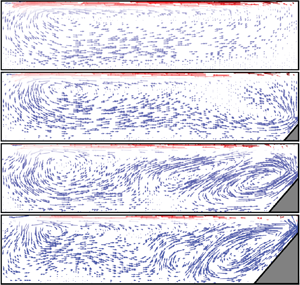
As previously mentioned, we do not focus on the local structures of this system. Nevertheless, the flow structures for different tidal frequencies can qualitatively exhibit the features of the different regimes of this system. Thus, we present the velocity vectors for different $\omega$ in figure 13. We find that for the buoyancy-controlled regime, the downwelling flows induced by plume emissions are the most significant fluid motion in the system. As the tidal frequency decreases, one can observe an overall enhancement of the flow strength. When the system enters the tide-controlled regime, the downwelling flow underneath the cold plate is no longer dominant. The flow in the vicinity of topography becomes strong. In some cases, these flows can be even stronger than those in the plume-emitting region (such as $\omega =0.04$ for $h/H=0.75$). The mean flow strength of the system keeps increasing as $\omega$ decreases until the system enters the drag-controlled regime. Comparing $\omega =0.04$ (corresponding to the tide-controlled regime) and $\omega =0.01$ (corresponding to the drag-controlled regime), one can see that either flow structure or flow strength in these two cases are very similar. Such a result suggests that the flow strength becomes independent on tidal frequency when the system enters the drag-controlled regime.

Figure 13.

Temporally averaged velocity vectors for $h/H=0.25$ (a) and $h/H=0.75$ (b). The velocity vectors are coloured according to the local temperature $\theta$. The length of the vectors are proportional to the velocity magnitude. Different shaded regions denote different flow regimes.

4.7. Mixing efficiency

In this section, we discuss the mixing efficiency $\eta$ defined by (3.5). The dependence of $\eta$ as a function of $\omega$ is shown in figure 14. For large $\omega$, different topographies converge to the same value which is $\eta _{HC}$. This can be explained by the results discussed previously that both global dissipation $\mathcal {E}$ and $G(APE)$, indicated by $Nu$, are insensitive to either topography height or tidal frequency $\omega$ in the buoyancy-control regime. The constant $\eta _{HC}$ (${\approxeq }0.85$) is much larger than the empirical value 0.2 used in most models for oceanic circulations. This high mixing efficiency is comparable with the results from other studies considering only buoyancy force (Scotti & White Reference Scotti and White2011; Sohail et al. Reference Sohail, Gayen and Hogg2018; Wang et al. Reference Wang, Huang and Xia2018). A transition to the tide-control regime occurs when $\omega \approx \omega _b$, after which $\eta$ decreases with $\omega$. From (3.5), one can obtain

(4.5a)$$\begin{gather} \frac{\partial\eta}{\partial G(APE)}=\frac{\mathcal{E}}{(\phi_d+\phi_\tau)^2}, \end{gather}$$

(4.5b)$$\begin{gather}\frac{\partial\eta}{\partial\phi_\tau}={-}\frac{\phi_d-\phi_i}{(\phi_d+\phi_\tau)^2 } . \end{gather}$$

Equation (4.5) shows that $\eta$ increases with $G(APE)$ but decreases when $\phi _\tau$ increases. The numerators in (4.5a) and (4.5b) correspond to the two irreversible energy transfer rates in this system and together form the denominator of $\eta$. As shown in figure 14, most of the results have $\eta >0.5$, which implies that $\phi _d-\phi _i>\mathcal {E}$. Thus, (4.5) suggests that $\eta$ is more sensitive to $\phi _\tau$ than $G(APE)$. Furthermore, as shown in figures 5 and 8, both $\phi _\tau$ and $Nu$ increase as $\omega$ decreases, and note that $Nu$ is proportional to $G(APE)$. One can further find that $\phi _\tau$ is much more sensitive to the changes of $\omega$ than $G(APE)$ is. Recalling that $\eta$ is more sensitive to $\phi _\tau$ than $G(APE)$ and decreases as $\phi _\tau$ increases, this explains the results that $\eta$ decreases as $\omega$ decreases. We also observe at a certain range of $\omega$ in the tide-control regime ($\omega >\omega _b$), higher topography yields smaller $\eta$, which shows that global dissipation is more sensitive than $G(APE)$ (or $Nu$) to $h/H$ as well. When $\omega$ decreases further, the system enters the drag-control regime. In this regime, both $G(APE)$ and $\epsilon _v$ become less sensitive to $\omega$. As a result, $\eta$ gradually stops decreasing with $\omega$ and asymptotically approaches to a saturated constant.

Figure 14.

Mixing efficiency $\eta$ as a function of $\omega /\omega _b$ for different $h/H$. The horizontal dashed line represents the mixing efficiency in the absence of tide and topography, and the vertical dashed line represents $\omega /\omega _b=1$.

To better explain the results of mixing efficiency shown in figure 14, we present the results of the local mixing rate $\phi _d(x,z)=(\textrm {d}z^*/\textrm {d}\theta )|\boldsymbol {\nabla }\theta |^2$ normalized by $\phi _d$ and local mixing efficiency (Sohail et al. Reference Sohail, Gayen and Hogg2018)

(4.6)\begin{equation} \eta_L\equiv\frac{\phi_d(x,z)}{\phi_d(x,z)+\epsilon_v(x,z)} \end{equation}

in figure 15. Figure 15(a) shows the normalized local mixing rate for $\omega =0.4$, which corresponds to the buoyancy-control regime. Mixing is significant at two regions: one is the region underneath the cold plate, where plumes emit and generate downwelling flow; the other is the thermocline adjacent to the upper boundary. When the tidal frequency decreases to $\omega =0.1$, which is the transitional frequency from the buoyancy-control to tide-control regime, we observe a tongue-like region with strong mixing near the topography, which is induced by the tide–topography interaction. Except for this point, the distribution of $\phi _d(x,z)/\phi _d$ is qualitatively similar to that of $\omega =0.4$. We then compare figure 15(b,c), both of which correspond to the tide-control regime. One can find that the high-mixing regions underneath the cold plate and near topography extend as $\omega$ decreases, which suggests the increase of the global mixing rate. Such extension is stopped when the system enters the drag-control regime (see figure 15d). The results shown in figure 15 imply that in the tide-control regime, mixing is enhanced when $\omega$ decreases ($U_{tide}$ increases); but in both the buoyancy- and drag-control regimes, mixing is insensitive to the change of $\omega$. Recalling that $Nu$ is proportional to $G(APE)$ and $\phi _d$, this result is consistent with the observed $Nu$ in figure 8. However, one should also be reminded that the enhancement in mixing does not mean an increase of the mixing efficiency. From the distribution of the local mixing efficiency $\eta _L$ shown in figure 15(e–h), we can see that the $\eta _L$ overall decreases as $\omega$ decreases in the right half of figure 15. This suggests that decreasing $\omega$ (increasing $U_{tide}$) induces a more significant enhancement in $\epsilon _v$ than $\phi _d$, which is consistent with the results shown in figures 4, 8 and 14. In another word, the tidal force is more effective in driving than the mixing fluid.

Figure 15.

Temporal averaging of the normalized local mixing rate $\phi _d(x,z)/\phi _d$ in log scale (left half) and local mixing efficiency $\eta _L$ (right half) for $h/H=0.75$ and (a) $\omega =0.4$, (b) $0.1$, (c) $0.04$ and (d) $0.01$.

As mixing in this system is sustained by two energy sources, the buoyancy and the tide, it may be illuminating to examine $\eta$ in terms of the relative strength of the driving forces. The quantities that are related to the two types of energies are $G(APE)$ and $\phi _\tau$, respectively. We first rewrite (3.5) using (3.3):

(4.7)\begin{equation} \eta=\frac{G(APE)-\phi_i}{G(APE)}\frac{G(APE)}{G(APE)+\phi_\tau}=\eta'\frac{G(APE)}{G(APE)+\phi_\tau}, \end{equation}

where $\eta '=(G(APE)-\phi _i)/G(APE)$ is formally the same as the mixing efficiency for a classical HC system in the absence of tidal force. However, here in $\eta '$, both $\phi _i$ and $G(APE)$ depend on $\omega$. Because $\phi _i$ is small compared with $G(APE)$ for sufficiently large $Ra$ (Peltier & Caulfield Reference Peltier and Caulfield2003; Gayen et al. Reference Gayen, Griffiths, Hughes and Saenz2013), $\eta '$ asymptotically approaches its upper limit of 1 as $Ra$ increases. For this reason, it is reasonable to neglect the $\omega$-dependence in $\eta '$ and we have $\eta '\approx \eta (\phi _\tau =0)=\eta _{HC}$. Then, (4.7) can be simplified as

(4.8)\begin{equation} \eta\approx\frac{\eta_{HC}}{1+\mathcal{R}}, \end{equation}

where $\mathcal {R}=\phi _\tau /G(APE)$. Equation (4.8) shows that for fixed $Ra$, the mixing efficiency can be expressed as a function of a single variable $\mathcal {R}$, which is the ratio of the mechanical driving over the energy arising from the buoyancy. In the present study, the mechanical driving is in the form of tidal energy, but wind shearing and other forms of mechanical forcing can also be included in $\phi _\tau$. Figure 16 shows the normalized mixing efficiency $\eta /\eta _{HC}$ as a function of $\mathcal {R}$. As shown in the figure, results for different $h/H$ collapse on a single curve which can be well described by the function $1/(1+\mathcal {R})$ without any adjustable parameter (represented by the dashed line in the figure). The slight deviation of this curve from the data may be attributed to the weak $\omega$ dependence of $\eta '$, which was neglected in obtaining (4.8).

Figure 16.

Graph of $\eta /\eta _{HC}$ as a function of $\mathcal {R}$ for different $h/H$. The blue star refers to the oceanic estimation. Black dashed line represents $\eta /\eta _{HC}=1/(1+\mathcal {R})$.

Examining $\eta$ in terms of $\mathcal {R}$ helps us to better understand the relationship between mixing and energy input. The generation rate of APE is estimated at 0.5 TW (Tailleux Reference Tailleux2009), while tidal and wind driving individually contribute approximately 1 TW to the MOC (Munk & Wunsch Reference Munk and Wunsch1998; Wunsch & Ferrari Reference Wunsch and Ferrari2004). Because $\eta _{HC}$ approaches 1 as $Ra$ increases, it is reasonable to assume $\eta _{HC}\approx 1$ for the ocean, the Rayleigh number of which is up to $10^{26}$ (Sohail et al. Reference Sohail, Gayen and Hogg2018). Substituting these values into (4.8), we estimate the global mixing efficiency to be 0.2, which is consistent with the empirical value. The case for ocean interior is represented by the blue star in figure 16. Globally, to achieve a mixing efficiency down to 0.2, the system must be controlled by mechanical sources. However, by comparing results for different topographies, we wish to point out that the local mixing efficiency strongly depends on the local environment. Features like topography, latitude, local tidal forcing strength can all significantly affect the ratio of mechanical force over the buoyancy one. As a result, the mixing efficiencies of different locations can vary significantly. Looking at it in another way, whether at a specific location, the driving is dominated by mechanical or thermal sources can now be inferred from the local mixing efficiency. The mixing efficiency of the Southern Ocean is estimated to be approximately 0.75–0.80 (Sohail et al. Reference Sohail, Gayen and Hogg2018), which suggests that the thermal driving can be more important than the mechanical one in those locations. This result is consistent with the fact that the tidal currents are generally weak in the Southern Ocean (Poulain & Centurioni Reference Poulain and Centurioni2015).

We now discuss the behaviour of $\mathcal {R}$ as a function of $\omega$, which is shown in figure 17. One sees that $\mathcal {R}$ has a similar dependence on $\omega$ as $\phi _\tau$ shown in figure 5. For this reason, we fit $\mathcal {R}$ using a function similar to (4.2), i.e. $\mathcal {R}=\mathcal {R}_\infty /(1+B\omega +{\omega ^2}/{\omega _t^2})$. The saturated value $\mathcal {R}_\infty$ of the energy ratio is the only fitting parameter here, because both $B$ and $\omega _t$ are the same parameters that have been obtained in the fitting of (4.2) (see also figure 5). The best fits of this equation are shown as the dashed curves in figure 17. The fact that $\mathcal {R}$ and $\phi _\tau$ can be described by a similar equation shows that $G(APE)$ has a relatively weak dependence on $\omega$.

Figure 17.

Graph showing $\mathcal {R}$ as a function of $\omega$. The dashed curves correspond to the best fit of equation $\mathcal {R}=\mathcal {R}_\infty /(1+B\omega +\omega ^2/\omega _t^2)$.

Figure 17 shows that for the tide- and buoyancy-control regimes with $\omega >\omega _t$, $\mathcal {R}$ follows a power law relationship $\omega ^{-2}$, and so we can write $\mathcal {R}\approx \mathcal {R}_\infty \omega _t^2/\omega ^2=\mathcal {R}_\infty Re_{tide}^2/Re_{tide}(\omega _t)^2$. Substitute this into (4.8), we obtain the following relation:

(4.9)\begin{equation} \gamma\equiv\frac{\eta}{\eta_{HC}-\eta}\approx\frac{1}{\mathcal{R}_\infty}\left(\frac{Re_{tide}}{Re_{tide}(\omega_t)}\right)^{{-}2}\quad(Re_{tide}< Re_{tide}(\omega_t)). \end{equation}

For sufficiently large values of $Ra$ and high turbulence intensity, $\eta _{HC}\approx 1$ and the mixing efficiency $\eta$ approximately equals the flux Richardson number $R_f$ (Peltier & Caulfield Reference Peltier and Caulfield2003; Gregg et al. Reference Gregg, D'Asaro, Riley and Kunze2018). Thus, (4.9) can be written as

(4.10)\begin{equation} \gamma_{R_f}\equiv\frac{R_f}{1-R_f}\approx\gamma\sim Re_{tide}^{{-}2}, \end{equation}

where $\gamma _{R_f}$ is the mixing coefficient, which is an important parameter in ocean models used to estimate the diapycnal buoyancy flux and diapycnal diffusivity (Gregg et al. Reference Gregg, D'Asaro, Riley and Kunze2018). Equations (4.9) and (4.10) yield a scaling relation of the mixing coefficient $\gamma _{R_f}\sim Re_{tide}^{-2}$ in the tide- and buoyancy-control regimes. We plot $\gamma$ as a function of $Re_{tide}$, and $\mathcal {R}_\infty \gamma$ as a function of $Re_{tide}/Re_{tide}(\omega _t)$ in figures 18(a) and 18(b), respectively. It shows that $\gamma$ follows the scaling relationship $\gamma _{R_f}\sim Re_{tide}^2$ for $Re_{tide}/Re_{tide}(\omega _t)<1$. However, as shown in 18(a), most of our cases have magnitudes much larger than the mixing coefficient $\gamma _{R_f}$ of the ocean, which is usually less than one (Gregg et al. Reference Gregg, D'Asaro, Riley and Kunze2018). This discrepancy with the field observation may be attributed to the limited parameter range of the current study. One of the consequences is that the approximation $\gamma _{HC}\approx 1$ may not hold for limited $Ra$. In fact, for the Rayleigh number we used in this study ($Ra=1\times 10^{10}$), we obtain $\gamma _{HC}=0.85$, which is probably not sufficiently close to 1. Another consequence is related to the magnitude of $\eta$. Considering the transitional state between the buoyancy- and tide-control regimes where the flow strengths driven by tidal and surface thermal forcings are comparable (i.e. $Re_{tide}$ equals to the Reynolds number in a classical HC system in the absence of tide), because the tidal force does not greatly enhance the heat transfer, one can estimate $G(APE)$ according to the power law relationship of $Nu$ for a classical HC system as $G(APE)\sim Nu\sim Ra^{0.2}$ (Rossby Reference Rossby1965; Shishkina et al. Reference Shishkina, Grossmann and Lohse2016). In a classical HC system, the Reynolds number has a scaling relationship $Re\sim Ra^{0.4}$ (Mullarney et al. Reference Mullarney, Griffiths and Hughes2004). Because the tidal velocity is comparable to the background flow, one can obtain $\phi _\tau \sim Re_{tide}^2\sim Ra^{0.8}$. One can find that the tidal power increases much faster than $G(APE)$ as $Ra$ increases. As a result, the mixing efficiency $\eta$ will decrease and yields a value of $\gamma$ closer to the mixing coefficient of the ocean $\gamma _{R_f}$. Thus, we expect that $\gamma$ will be closer to $\gamma _{R_f}$ for higher $Ra$, and examining the power law relationship (4.10) in simulations or experiments with higher $Ra$ could be one of the goals in future studies.

Figure 18.

Graph showing (a) $\gamma$ and (b) $\mathcal {R}_\infty \gamma$ as a function of $Re_{tide}/Re_{tide}(\omega _t)$ for different $h/H$. In panel (b), the inclined black dashed line represents $[Re_{tide}/Re_{tide}(\omega _t)]^{-2}$, and the red dash–dotted line refers to $Re_{tide}=Re_{tide}(\omega _t)$.

It is seen from figure 18 that for large $Re_{tide}$ and for some cases with $h/H=0$ and $0.25$, the value of $\gamma$ can be smaller than 1, which is in the range of $\gamma _{R_f}$ observed in the ocean. However, we cannot thus draw the conclusion that the ocean is within the drag-control regime. To see this, we estimate the typical ocean current speed by first assuming a buoyancy driven background flow. The flow strength in such a case is given by $Re=CRa^{0.4}$, where $C$ is a constant to be determined. Using the value of $Re$ in the absence of topography and tidal force, we determine the constant $C=0.034$. Thus, when buoyancy is the only energy source, the velocity of the thermocline is given by $U_{thermo}\approx CRa^{-0.1}\sqrt {\alpha gL\Delta Pr}$. We take $g={9.8}\ \textrm {m}\ \textrm {s}^{-2}$, $\alpha ={1\times 10^{-4}}\ \textrm {K}^{{-1}}$ (Sohail et al. Reference Sohail, Gayen and Hogg2018), $L=1\times 10^{7}\ \textrm {m}$, $\varDelta ={10}\ \textrm {K}$, $\kappa ={1\times 10^{-7}}\ \textrm {m}^2\ \textrm {s}^{-1}$ and $\nu =1\times 10^{-6}\ \textrm {m}^2\ \textrm {s}^{-1}$ (Siggers, Kerswell & Balmforth Reference Siggers, Kerswell and Balmforth2004). Thence, we estimate $U_{thermo}\approx 2\ \textrm {cm}\ \textrm {s}^{-1}$ if the ocean current is driven by thermal forcing. As for the tidal current, the Global Drifter Program (GDP) data shows that the M2 (semidiurnal) currents in the open-ocean areas are $3 - 5\ \textrm {cm}\ \textrm {s}^{-1}$ (Poulain & Centurioni Reference Poulain and Centurioni2015), which suggests that the tide is the dominant energy source in such areas of the ocean. However, in the deep tropics and South Pacific, for example, the M2 currents are small (${<}\,2\ \textrm {cm}\ \textrm {s}^{-1}$). Thus, in these areas, buoyancy could be the dominant governing mechanism.