1 Introduction
Geological activity is a consequence of the convective motions that develop in the Earth’s mantle. In order to understand how it is generated, forward models of convection of increasing complexity have multiplied over the years (e.g. McKenzie, Roberts & Weiss Reference McKenzie, Roberts and Weiss1973; Christensen & Hofmann Reference Christensen and Hofmann1994; Samuel & Farnetani Reference Samuel and Farnetani2003; Nakagawa & Tackley Reference Nakagawa and Tackley2014). These models are, however, inherently questionable because of fundamental uncertainties on the sources and amount of energy involved. According to recent studies (e.g. Jaupart et al. Reference Jaupart, Labrosse, Lucazeau and Mareschal2015), approximately half of the Earth’s heat loss today is due to secular cooling at a rate of approximately 100 K per billion years and the other half comes from the radioactive decay of uranium, thorium and potassium in silicate rocks of the crust and mantle. Large uncertainties arise when one attempts to focus on the mantle, since the amount of heat received from the core, induced by its secular cooling, remains poorly constrained (Labrosse, Poirier & Le Mouël Reference Labrosse, Poirier and Le Mouël2001; Lay et al. Reference Lay, Hernlund, Garnero and Thorne2006; Cottaar & Buffett Reference Cottaar and Buffett2012; Gomi et al. Reference Gomi, Ohta, Hirose, Labrosse, Caracas, Verstraete and Hernlund2013). This has led to models that can be described as semi-empirical because they rely heavily on current observations such as the motions of surface plates and the distribution of internal density anomalies deduced from gravity and seismological studies (Mitrovica & Forte Reference Mitrovica and Forte2004; Deschamps & Tackley Reference Deschamps and Tackley2008, Reference Deschamps and Tackley2009). These models are focused on the current convection regime and incorporate most of the available constraints, implying that they are difficult to test and ill-suited for studies of planetary evolution back in time (Bello et al. Reference Bello, Coltice, Rolf and Tackley2014). An alternative strategy has been to try to infer the controls on convective motions from the observations themselves. For instance, Deschamps, Rogister & Tackley (Reference Deschamps, Rogister and Tackley2018) have proposed to constrain the presence of chemical heterogeneities at the base of the Earth’s mantle with the topography of the core–mantle boundary, while Mitrovica & Forte (Reference Mitrovica and Forte2004) have combined models of Earth’s mantle convection with glacial isostatic adjustment data to infer the mantle viscosity profile. On Earth, however, one runs the risk of being mistaken because of the many complicating factors involved, which include the presence of continents or multiple mantle phase changes (e.g. Gurnis Reference Gurnis1988; Guillou & Jaupart Reference Guillou and Jaupart1995; Tackley Reference Tackley, Gurnis, Wysession, Knittle and Buffett1998b ; Stixrude & Lithgow-Bertelloni Reference Stixrude and Lithgow-Bertelloni2011; Rolf, Coltice & Tackley Reference Rolf, Coltice and Tackley2012). Thus, whether all the available observations form a self-consistent set, such that they can all be accounted for by the workings of a single convective system, is an important issue. In silicate planets other than Earth, one has to work with fewer observations but, with a sound understanding of the characteristics of convection, one can still make useful inferences. For example, the main features of the gravity field and surface topography on Venus have been explained by a small number of mantle plumes, nine to be precise, over a uniform background (Smrekar & Sotin Reference Smrekar and Sotin2012). If this inference is valid, it leads to powerful constraints on the energy budget and interior viscosity of the planet.
In studies of silicate planets and planetary bodies, one cannot draw only from the comprehensive body of knowledge that is available for Rayleigh–Bénard convection because interior motions are largely driven by internal heat sources instead of heat supplied to the base. Heat sources include long-period radionuclides as well as contributions from secular cooling and tidal heating, although the latter is only dominant in some planetary bodies such as the icy satellites of Saturn and Jupiter (Hussmann et al. Reference Hussmann, Choblet, Lainey, Matson, Sotin, Tobie and Van Hoolst2010; Schubert et al. Reference Schubert, Hussmann, Lainey, Matson, McKinnon, Sohl, Sotin, Tobie, Turrini and Van Hoolst2010). In spite of their relevance to planetary evolution, studies of internally heated convective systems have lagged behind those for Rayleigh–Bénard set-ups (Goluskin Reference Goluskin2015). Moreover, such systems are particularly interesting from theoretical and physical perspectives because they involve a single unstable thermal boundary layer that is not affected by motions generated at another boundary (Goluskin & Spiegel Reference Goluskin and Spiegel2012; Seis Reference Seis2013; Goluskin Reference Goluskin2015). For instance, this may enable us to better capture the dynamics of the thermal boundary layer, especially the mechanisms generating downwellings and upwellings.
For a fluid layer with internal heating rate
 $H$
above an adiabatic base, dimensional analysis of the mass, momentum and energy conservation equations in the Boussinesq (Reference Boussinesq1903) approximation leads to two dimensionless numbers, the Rayleigh–Roberts number
 $Ra_{H}$
and the Prandtl number
 $Pr$
(Roberts Reference Roberts1967; Schubert, Turcotte & Olson Reference Schubert, Turcotte and Olson2001):
 $$\begin{eqnarray}\displaystyle & \displaystyle Ra_{H}={\displaystyle \frac{\unicode[STIX]{x1D70C}g\unicode[STIX]{x1D6FC}Hd^{5}}{\unicode[STIX]{x1D702}\unicode[STIX]{x1D705}k}}, & \displaystyle\end{eqnarray}$$
 $$\begin{eqnarray}\displaystyle & \displaystyle Pr={\displaystyle \frac{\unicode[STIX]{x1D702}}{\unicode[STIX]{x1D70C}\unicode[STIX]{x1D705}}}, & \displaystyle\end{eqnarray}$$
where
 $\unicode[STIX]{x1D70C}$
is the density,
 $g$
the acceleration of gravity,
 $\unicode[STIX]{x1D6FC}$
the thermal expansion coefficient,
 $d$
the thickness of the fluid layer,
 $\unicode[STIX]{x1D702}$
viscosity,
 $\unicode[STIX]{x1D705}$
thermal diffusivity and
 $k$
thermal conductivity. Note that all fluid properties are taken in the reference state. The influence of the Prandtl number has only been investigated in a cursory fashion, despite the very large gap that exists between values for water (
 $Pr\approx 7$
), the most common experimental fluid, and for the solid interior of silicate planets (
 $Pr>10^{21}$
). In the latter, convection is in a laminar regime even at very large values of
 $Ra_{H}$
and it is appropriate to work in the limit of infinite
 $Pr$
(Schubert et al.
Reference Schubert, Turcotte and Olson2001).
For values of
 $Ra_{H}$
up to
 $10^{5}$
, steady-state motions are organized in periodic planforms that become increasingly complex as the Rayleigh–Roberts number is increased. For
 $Pr\approx 7$
, these planforms have been explored systematically in laboratory experiments (Tritton & Zarraga Reference Tritton and Zarraga1967; Kulacki & Nagle Reference Kulacki and Nagle1975; Kulacki & Emara Reference Kulacki and Emara1977; Takahashi et al.
Reference Takahashi, Tasaka, Murai, Takeda and Yanagisawa2010) and numerical simulations (Ichikawa et al.
Reference Ichikawa, Kurita, Yamagishi and Yanagisawa2006; Glover & Generalis Reference Glover and Generalis2009). Ordered by
 $Ra_{H}$
value, they take the form of squares, hexagons, both with an axial downwelling, and finally spokes, i.e. hexagons with an axial downwelling that is star-shaped instead of cylindrical. Their horizontal wavelength increases with
 $Ra_{H}$
in a phenomenon called ‘cell dilatation’. The same planforms are observed at larger
 $Pr$
values, as shown by both laboratory experiments (
 $3\times 10^{2}\leqslant Pr\leqslant 3\times 10^{4}$
) and numerical simulations in the infinite
 $Pr$
limit (Carrigan Reference Carrigan1982, Reference Carrigan1985; Houseman Reference Houseman1988; Parmentier & Sotin Reference Parmentier and Sotin2000; Limare et al.
Reference Limare, Vilella, Di Giuseppe, Farnetani, Kaminski, Surducan, Surducan, Neamtu, Fourel and Jaupart2015), but it seems that cell dilatation does not occur. Moreover, their stability domains appear to be different from those for
 $Pr\approx 7$
, but have not been determined precisely yet (Davaille & Limare Reference Davaille and Limare2015).
Very few studies have been made for intermediate values of
 $Ra_{H}$
in the
 $10^{5}{-}10^{6}$
range (Limare et al.
Reference Limare, Vilella, Di Giuseppe, Farnetani, Kaminski, Surducan, Surducan, Neamtu, Fourel and Jaupart2015), despite the dramatic change of convection planform that is observed. Most of studies focus on cases with
 $Ra_{H}\gtrsim 10^{6}$
where convective motions become time-dependent. In this regime, scaling laws for the thickness of the upper thermal boundary layer and for the temperature difference across it have been derived from simple dimensional considerations and have been compared successfully to numerical and laboratory results (Cheung Reference Cheung1977; Kulacki & Emara Reference Kulacki and Emara1977; Parmentier & Sotin Reference Parmentier and Sotin2000; Limare et al.
Reference Limare, Vilella, Di Giuseppe, Farnetani, Kaminski, Surducan, Surducan, Neamtu, Fourel and Jaupart2015; Vilella & Kaminski Reference Vilella and Kaminski2017). In addition, scaling arguments and direct numerical simulations in the infinite
 $Pr$
limit indicate that the number of downwellings per unit area is proportional to
 $Ra_{H}^{1/4}$
(Parmentier & Sotin Reference Parmentier and Sotin2000).
Here, we aim at filling gaps in our understanding of laminar convection in internally heated horizontal fluid layers above an adiabatic base. This work builds on two previous studies (Limare et al.
Reference Limare, Vilella, Di Giuseppe, Farnetani, Kaminski, Surducan, Surducan, Neamtu, Fourel and Jaupart2015; Vilella & Kaminski Reference Vilella and Kaminski2017). Limare et al. (Reference Limare, Vilella, Di Giuseppe, Farnetani, Kaminski, Surducan, Surducan, Neamtu, Fourel and Jaupart2015) have compared the characteristics of convective flows in the laboratory at large
 $Pr$
values (
 $3\times 10^{2}<Pr<3\times 10^{4}$
) and in direct numerical simulations in the infinite
 $Pr$
limit with exactly the same tank dimensions and temperature-dependent fluid properties. They have observed the same planforms in both types of studies and have shown that the thickness and temperature difference across the upper boundary layer scale as
 $Ra_{H}^{-1/4}$
down to surprisingly small values of
 $Ra_{H}$
(
 ${\approx}8\times 10^{5}$
). Vilella & Kaminski (Reference Vilella and Kaminski2017) have focused on the upper thermal boundary layer and have shown that it hosts large lateral temperature variations even at high
 $Ra_{H}$
values, with important implications for magma generation in silicate planets. Using high-precision three-dimensional (3-D) direct numerical simulations in the infinite
 $Pr$
limit, they have established scalings for both the horizontally averaged structure and the hottest regions of the upper thermal boundary layer. In this paper, we use the same numerical runs and add seven new ones to extract a comprehensive and consistent data set of thermal and flow characteristics, focusing on cold downwellings for the latter, over a very large range of Rayleigh–Roberts numbers (
 $5\times 10^{3}{-}10^{9}$
). We determine precisely the various planforms that occur, their domains of existence, their geometrical shapes and average dimensions. We document how the thermal structure of the fluid layer evolves as the Rayleigh–Roberts number increases. We also derive scaling laws for several variables of great geophysical interest, such as the average plume size and vertical velocity and the amplitude of thermal anomalies in the fluid interior, and compare them successfully to numerical results. We consider two sets of mechanical boundary conditions (free slip or rigid) in order to investigate how the interior convective motions depend on the dynamics of the unstable boundary layer at the top.
The paper is organized as follows. We begin by describing the various planforms of convection that are generated at the top of the layer and determine their respective domains of existence as a function of
 $Ra_{H}$
. We investigate how motions in the fluid interior are related to the shallow planform. We then determine the main characteristics of the cold downwellings that are generated at the upper boundary and that go through the fluid layer and propose simple scaling laws for them. In a final section, we discuss some implications of our results for studies of the Earth and other planetary bodies.
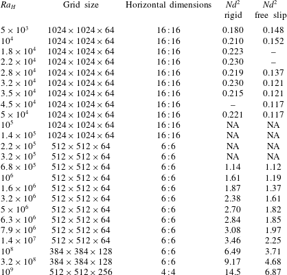
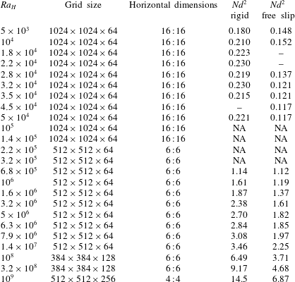
Input parameters for the 45 numerical simulations analysed in this paper: the Rayleigh–Roberts number (
 $Ra_{H}$
), the number of grid elements used in X : Y : Z directions, the horizontal dimensions X : Y (scaled to the fluid layer thickness).
 $Nd^{2}$
is the dimensionless number of downwellings per unit area at mid-depth (see text). ‘NA’ indicates that it was not possible to obtain a reliable count of downwellings; ‘–’ indicates that no calculation was carried out.
2 Numerical simulations
We consider an incompressible fluid layer heated internally and cooled from above in the Boussinesq (Reference Boussinesq1903) approximation and in the infinite
 $Pr$
limit. The top boundary is kept at a constant temperature set to zero and the bottom one is adiabatic. We seek scaling laws that encapsulate the main physical aspects of the flow in compact form, which is best achieved for fluids with constant physical properties. Identical boundary conditions, which are either free slip or rigid, are imposed at the top and bottom. This is done to investigate the impact of boundary conditions on the dynamics of the thermal boundary layer (TBL) at the top and on the convective motions in the fluid interior. Using the following scales,
 $d$
for spatial coordinates,
 $d^{2}/\unicode[STIX]{x1D705}$
for time,
 $\unicode[STIX]{x1D705}/d$
for velocity,
 $\unicode[STIX]{x1D702}\unicode[STIX]{x1D705}/d^{2}$
for pressure and finally
 $Hd^{2}/k$
for temperature, the conservation equations are written in dimensionless form as follows:
 $$\begin{eqnarray}\displaystyle & \displaystyle 0=\unicode[STIX]{x1D735}\boldsymbol{\cdot }\boldsymbol{v}, & \displaystyle\end{eqnarray}$$
 $$\begin{eqnarray}\displaystyle & \displaystyle 0=-\unicode[STIX]{x1D735}P+\unicode[STIX]{x1D6FB}^{2}\boldsymbol{v}+Ra_{H}T\boldsymbol{n}_{\boldsymbol{z}}, & \displaystyle\end{eqnarray}$$
 $$\begin{eqnarray}\displaystyle & \displaystyle {\displaystyle \frac{\text{D}T}{\text{D}t}}={\displaystyle \frac{\unicode[STIX]{x2202}T}{\unicode[STIX]{x2202}t}}+\boldsymbol{v}\boldsymbol{\cdot }\unicode[STIX]{x1D735}T=\unicode[STIX]{x1D6FB}^{2}T+1, & \displaystyle\end{eqnarray}$$
where
 $\boldsymbol{v}$
,
 $P$
and
 $T$
are velocity, pressure and temperature, respectively, and where
 $t$
is time and
 $\boldsymbol{n}_{\boldsymbol{z}}$
the unit vector in the vertical direction. Calculations were performed in 3-D Cartesian geometry using Stag3D (Tackley Reference Tackley1998a
, Reference Tackley2008), a robust code that has been tested thoroughly against several others. Time-stepping is implemented for the heat equation using a finite volume formulation and the mass and momentum conservation equations are solved using a finite difference multigrid technique. The accuracy of this code was assessed by a detailed comparison with laboratory experiments (Limare et al.
Reference Limare, Vilella, Di Giuseppe, Farnetani, Kaminski, Surducan, Surducan, Neamtu, Fourel and Jaupart2015) and precision tests are described in the supplementary material available at https://doi.org/10.1017/jfm.2018.316. We have run a large number of numerical simulations in order to determine the characteristics of convection over a wide
 $Ra_{H}$
range (table 1). We made sure that the calculations allow excellent resolution of the temperature and velocity fields by decreasing the grid spacing as we increased the Rayleigh–Roberts number. At
 $Ra_{H}=10^{9}$
, the largest value of the Rayleigh–Roberts number studied, there are nine grid points through the thermal boundary layer. We also made sure that the horizontal resolution was optimal, such that the intricacies of the convection planform were adequately accounted for. We show in the supplementary material that results do not depend on grid size. In order to minimize lateral edge effects, computational domains had high aspect ratios (width over thickness) and reflecting vertical boundaries. The smallest aspect ratio was equal to 4 and was only used for calculations at the largest
 $Ra_{H}$
value (
 $Ra_{H}=10^{9}$
). In this case, convective motions develop over small horizontal spatial scales, such that the calculations allowed a representative statistical sampling of the complex flow field and such that the impact of the lateral boundaries was limited to narrow peripheral regions. In all other cases, aspect ratios were set at 6 or more (table 1). In a few cases, we checked that calculations for different aspect ratios lead to essentially identical results (see the supplementary material for a detailed comparison).
Calculations are time-dependent and are started from different initial conditions depending on the
 $Ra_{H}$
value. At low
 $Ra_{H}$
associated with steady-state regimes, the whole fluid layer is initially at a constant temperature with random, small amplitude, perturbations. This ensures that the convective planform of the steady-state solution does not depend on an arbitrary initial spatial pattern. At high
 $Ra_{H}$
, truly steady-state regimes cannot be achieved and time series of the local values of temperature and velocity exhibit fluctuations at all times. We therefore consider ‘statistical steady-state’ conditions, such that temperature and heat flux values remain within the same ranges over several ‘overturn times’. The overturn time is defined to be the time taken by a fluid parcel to go full circle, from the upper boundary layer to the base of the domain and then back up. For these calculations (high
 $Ra_{H}$
), the initial condition is the temperature field for a solution at a lower
 $Ra_{H}$
value, a strategy that significantly reduces the computation time. We checked that the final result does not depend on this initial condition in a few cases.
3 Convective planforms
3.1 Preliminary note
Before we describe the convective planforms in more detail, it is useful to recall how the characteristics of the upper thermal boundary layer depend on the model parameters, especially on the Rayleigh–Roberts number and on the boundary conditions. For
 $10^{5}\leqslant Ra_{H}\leqslant 10^{9}$
, the temperature difference and thickness of the boundary layer, noted
 $\unicode[STIX]{x0394}T_{TBL}$
and
 $\unicode[STIX]{x1D6FF}$
, respectively, are such that
 $$\begin{eqnarray}\displaystyle & \displaystyle {\displaystyle \frac{\unicode[STIX]{x0394}T_{TBL}}{Hd^{2}/k}}=C_{\unicode[STIX]{x0394}T}Ra_{H}^{-1/4}\quad \text{and}\quad {\displaystyle \frac{\unicode[STIX]{x1D6FF}}{d}}=C_{\unicode[STIX]{x1D6FF}}Ra_{H}^{-1/4}, & \displaystyle\end{eqnarray}$$
where
 $C_{\unicode[STIX]{x0394}T}$
and
 $C_{\unicode[STIX]{x1D6FF}}$
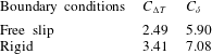
are proportionality constants that depend on the boundary conditions (Limare et al.
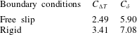
Reference Limare, Vilella, Di Giuseppe, Farnetani, Kaminski, Surducan, Surducan, Neamtu, Fourel and Jaupart2015, and see table 2). These relationships can be derived from local scaling arguments (Vilella & Kaminski Reference Vilella and Kaminski2017), indicating that the dynamics of the upper boundary layer is locally controlled, independently of the total fluid layer thickness. Note that thickness
 $\unicode[STIX]{x1D6FF}$
corresponds to the base of the boundary layer, which is defined with the horizontally averaged temperature at the point where the convective flux is maximum. An alternative definition relies on the heat flux through the upper boundary, such that
 $q=\unicode[STIX]{x0394}T_{TBL}^{\ast }/\unicode[STIX]{x1D6FF}^{\ast }$
in dimensionless variables. In steady state, heat conservation requires that
 $q=1$
, implying that
 $\unicode[STIX]{x1D6FF}^{\ast }=\unicode[STIX]{x0394}T_{TBL}^{\ast }$
. Limare et al. (Reference Limare, Vilella, Di Giuseppe, Farnetani, Kaminski, Surducan, Surducan, Neamtu, Fourel and Jaupart2015) chose the former definition in order to verify that the vertical temperature profile in the boundary layer conforms to local scalings. By contrast, for
 $Ra_{H}\leqslant 10^{5}$
the relationship (3.1) is no longer valid, indicating an interdependence between the upper boundary layer and the fluid interior. Another key result is that regardless of the
 $Ra_{H}$
value, beneath a rigid top, the boundary layer is significantly thicker and hosts a larger temperature difference than beneath a free slip surface. Variations of behaviour observed when changing the boundary conditions as well as the
 $Ra_{H}$
value are likely to affect the convective planforms. These differences will be identified and quantified in the following sections.
Proportionality constants in the scaling laws for the temperature difference and thickness of the upper thermal boundary layer (3.1) from Limare et al. (Reference Limare, Vilella, Di Giuseppe, Farnetani, Kaminski, Surducan, Surducan, Neamtu, Fourel and Jaupart2015).
Convective planform as a function of the Rayleigh–Roberts number (
 $Ra_{H}$
) for free slip boundaries at the top (
 $z=1$
) and bottom (
 $z=0$
). The temperature field is shown for a horizontal plane located at
 $z=0.9$
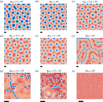
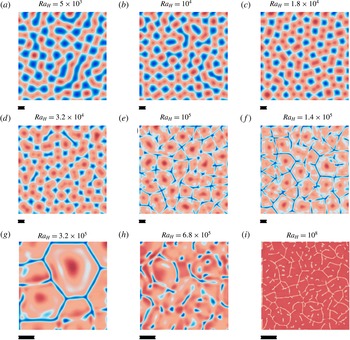
. Blue and red colours correspond to fluid that is colder and hotter than the horizontal average at that depth, respectively. The colour scale is not the same for all the panels in order to enhance visibility of the convective structure. The resolution and the domain aspect ratio are changed for panels (g–i) (table 1) due to the small dimensions of the convective cells. The black bar beneath each panel corresponds to the thickness of the fluid layer, i.e. the height of the computation domain.

Convective planform defined from the temperature field in figure 1(a) for
 $Ra_{H}=5\times 10^{3}$
(a) and in figure 1(e) for
 $Ra_{H}=5\times 10^{4}$
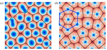
(b). Temperatures are shown as deviations from the local horizontal average, with blue and red standing for temperature that is colder and hotter than average, respectively. Black lines in both panels are the Voronoi tessellation, which indicates a dominantly hexagonal pattern. Thick blue lines in (b) illustrate how hexagons may form out of a spoke pattern, in that the case the centre downwelling would no longer be present.

3.2 Steady-state regimes
By definition, steady-state regimes are such that the geometrical pattern of convection does not change over time. It is difficult, however, to prove that true steady state has been achieved in numerical simulations, since it would require extremely long computation times. We consider that the solution is steady-state when the pattern of convection does not change significantly over several overturn times (which has been defined above). This requires a dimensionless computational time 5–50 with a typical value of
 ${\approx}10$
.
The analysis is carried out in a horizontal plane located at dimensionless height
 $z=0.9$
above the base. The flow field can be split into a number of ‘convective cells’, which are defined by one downwelling and its ‘capture’ area, i.e. the area in the upper boundary layer where fluid flows laterally towards the downwelling. For visualization purposes, we also use a Voronoi procedure in which each cell is built around one downwelling and includes all the points that are closer to it than to any other one.
We first discuss results obtained for free slip boundaries. Near the threshold value of
 $Ra_{H}$
for the onset of convection (
 $Ra_{H,cr}=868$
), the theoretical analysis by Roberts (Reference Roberts1967) indicates that three planforms are possible, described as 2-D rolls and hexagons with either an axial upwelling or an axial downwelling. By analogy with Rayleigh–Bénard systems, we may expect that hexagons with an axial downwelling are preferred over other ones due to the different thermal boundary conditions at the top and bottom (Cross & Hohenberg Reference Cross and Hohenberg1993). Our calculations confirm this (figures 1
a and 2). The preferential pattern is made of hexagons with a cylindrical downwelling at their centre, which have been called ‘down’ hexagons, but there are also a few pentagons and rare squares and heptagons.
As
 $Ra_{H}$
increases, the planform grades into a spoke pattern (figure 1
b–d). This pattern is still made of hexagons, but features an axial downwelling that is star-shaped instead of cylindrical, with six spokes perpendicular to the six sides of the encasing hexagon. The planform evolves progressively as
 $Ra_{H}$
increases, such that spokes extend to increasing distances from the hexagon centres. This makes it difficult to determine a threshold value for the Rayleigh–Roberts number that marks the appearance of this planform unambiguously. We have set the transition at the stage when the downwellings outlines become noticeably spiky (
 $Ra_{H}\approx 2.8\times 10^{4}$
, figure 1
c). This is obviously an approximate procedure, but the range of
 $Ra_{H}$
values for the transition is less than 0.2 log units, as may be seen from table 1 and figure 1(b,c).
Increasing
 $Ra_{H}$
further, the spokes become increasingly prominent and their tips eventually reach the sides of the encasing hexagons. This leads to a spectacular change of flow pattern that marks the onset of time-dependent convection (
 $Ra_{H}\approx 10^{5}$
figure 1
e,f).
3.3 The ‘sheet’ regime
For
 $Ra_{H}\gtrsim 10^{5}$
, the flow adopts a new configuration that is observed over a range of
 $Ra_{H}$
spanning approximately 0.3 log units for free slip boundaries and about 0.7 log units for rigid ones. Instead of continuous upwelling regions encircling individual downwellings, the flow gets organized in arrays of thin line downwellings that encapsulate broad upwellings (figure 1
f). These downwellings are no longer separated from one another by continuous upwelling areas and will be referred to as ‘sheets’. They converge to three-way junction nodes and outline a pattern suggestive of hexagons, but with a polarity that is the opposite of that for smaller values of the Rayleigh–Roberts number: they now occur along the sides of polygonal cells instead of at their centre, which was described as a switch from ‘down’ hexagons to ‘up’ hexagons by Carrigan (Reference Carrigan1985). This polarity reversal is associated with a marked increase of cell dimensions. This regime, which will be called the sheet regime, is of particular interest for reasons that will be explained later. Sheets are similar to ‘line plumes’ emanating from elongated regions in an unstable boundary layer, which are the predominant flow structure in turbulent Rayleigh–Bénard convection (Adrian, Ferreira & Boberg Reference Adrian, Ferreira and Boberg1986; Theerthan & Arakeri Reference Theerthan and Arakeri1994; Shishkina & Wagner Reference Shishkina and Wagner2008; Zhou & Xia Reference Zhou and Xia2010).
Two features make the sheet regime distinctive. One is that the length and spacing of sheets exceed the depth of the fluid layer by large amounts. It is unfortunately difficult to determine a representative length scale due to the irregular arrangement of the sheets, their variable lengths and their small number even in a domain that extends laterally over sixteen times the layer thickness. The other feature is that it is a time-dependent pattern, albeit one that evolves very slowly, such that the sheets move horizontally across the domain. The ‘drift’ velocity is smaller than the average vertical velocity by at least one order of magnitude. The sheet regime is therefore neither truly steady-state nor truly time-dependent. Nevertheless, for the sake of simplicity, we consider in the following the sheet regime as a steady-state regime.
3.4 Time-dependent flow regimes
For free slip boundaries, the sheet regime eventually segues into a time-dependent one with no obvious geometrical pattern when
 $Ra_{H}\approx 3.2\times 10^{5}$
(figure 1
h). The planform is shown at a dimensionless depth of 0.1 below the top, in the upper part of the boundary layer (
 $\unicode[STIX]{x1D6FF}=0.25$
in this particular case), corresponding to what would be seen by an external observer. It is ill-defined at that level but we shall see later that it changes as one probes deeper in the fluid and one can determine a meaningful spacing between adjacent downwellings. Individual sheet segments are unstable and develop into a number of discrete focused downwellings (figure 1
g). The lifetime of an individual sheet is smaller than the time scale of its lateral drift motion by approximately two orders of magnitude. Sheets are rarely isolated and belong to clusters made of nodal points and branches. With three sheets per nodal point on average, the pattern can be interpreted as a set of ‘truncated hexagons’ (figure 1
i for
 $Ra_{H}=10^{8}$
).
Convective planform as a function of the Rayleigh–Roberts number (
 $Ra_{H}$
) for rigid boundaries at the top (
 $z=1$
) and bottom (
 $z=0$
). The temperature field is shown for a horizontal plane located at
 $z=0.9$
. Blue and red colours correspond to fluid that is colder and hotter than the horizontal average at that depth, respectively. The colour scale is not the same for all the panels in order to enhance visibility of the convective structure. The resolution and the domain aspect ratio are changed for panels (g–i) (table 1) due to the small size of convective cells. The black bar beneath each panel corresponds to the thickness of the fluid layer, i.e. the box height. Note that the typical dimensions of the convective cells that are shown in (f) and (g) are very close to one another when scaled to layer thickness.

Diagram showing the change of convective planform as a function of the Rayleigh–Roberts number (
 $Ra_{H}$
) for both rigid (black bar) and free slip (red bar) boundaries. Threshold values of
 $Ra_{H}$
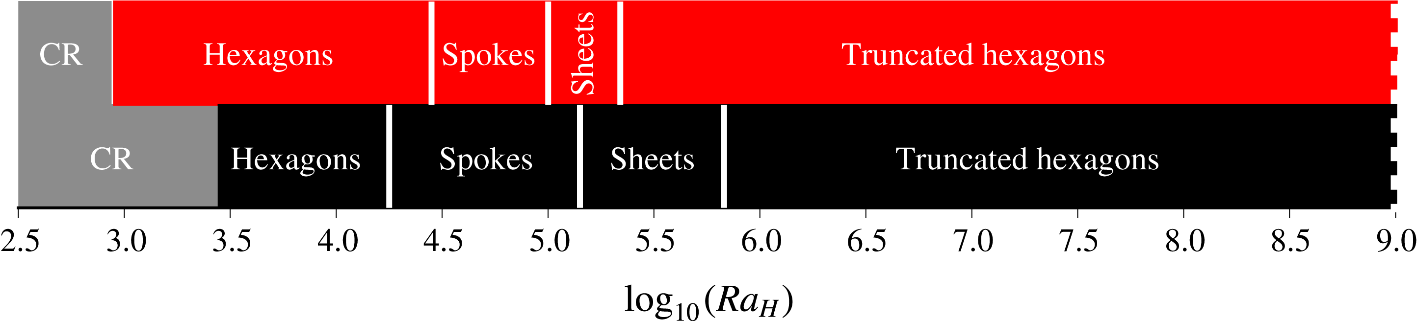
for the onset of convection come from stability analysis (Roberts Reference Roberts1967; Kulacki & Goldstein Reference Kulacki and Goldstein1975) and CR stands for conductive regime, whereas the other transitions are based on the present numerical simulations (figures 1 and 3).

3.5 Rigid boundaries
We use the same procedure and descriptive terms to characterize convective planforms between rigid boundaries. One notable difference is that downwellings are in larger numbers than in cases with free slip boundaries (figures 1 and 3). They are also wider. This second difference is, however, not apparent in figures 1 and 3, which illustrate the geometrical planforms at shallow depth, and will be shown by measurements of the cross-sectional area of downwellings in horizontal planes at mid-depth in the fluid interior. Downwellings are fed by laterally converging flows that extend through the upper boundary layer, and their size reflects the thickness of that boundary layer, which is thicker beneath a rigid boundary (table 2).
The planforms are essentially identical to those for free slip boundaries but the critical
 $Ra_{H}$
values for transitions are not the same (figure 4). This is not surprising as the critical value of
 $Ra_{H}$
for the onset of convection is larger for rigid boundaries (
 $Ra_{H,cr}=2772$
following Roberts Reference Roberts1967) than for free slip ones (
 $Ra_{H,cr}=868$
following Kulacki & Goldstein Reference Kulacki and Goldstein1975). The spoke and sheet regimes are observed over a wider
 $Ra_{H}$
range than with free slip boundaries. The sheet regime is heralded by a gradual change of planform illustrated in figure 3(d,e), which is such that gaps between neighbouring spokes get bridged progressively, leading to a polygonal array of line downwellings. As in cases with free boundaries, downwellings go from isolated plumes at cell centres to a continuous network of thin sheets encircling broad upwellings (figures 3
f,g). This can be described again as a switch from ‘down’ to ‘up’ hexagons with a marked increase of cell dimensions. This transition occurs at
 $Ra_{H}\approx 40\,Ra_{H,cr}\approx 10^{5}$
, which is consistent with the careful laboratory observations of Carrigan (Reference Carrigan1985).
For
 $Ra_{H}\geqslant 10^{6}$
(figure 3
i), the planform can be described again as a set of truncated hexagons, perhaps more convincing than in the free slip calculations. The vast majority of the downwelling sheets belong to networks that can be traced over large horizontal distances, with nodal points where three sheets converge. Such three-way junctions are consistent with a hexagonal pattern, but there are also a very small number of four-way junctions. Individual sheets typically undergo the following cycle. A new downwelling forms in the upper boundary layer and gets stretched towards an already existing sheet due to the horizontal flow that feeds it. Once several (generally three) downwelling sheets are joined in this manner, downward flow is amplified in the nodal area and draws fluid from the sheets, which coalesce and eventually disappear. This can be described as a hexagon-building process that does not go to completion. An important feature is that sheets are not stable structures as they go down in the fluid, as illustrated in the following section.
Temperature field (
 $T$
) within and around downwellings at different heights above base (
 $z=1$
is at the top) for different values of the Rayleigh–Roberts number (
 $Ra_{H}$
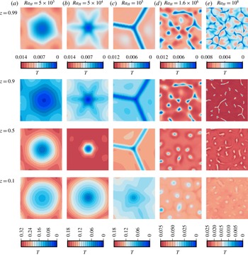
) in a fluid layer with free slip boundaries. All the panels extend over three times the fluid layer thickness in both horizontal directions. For a given Rayleigh–Roberts number, all panels are centred at the same horizontal coordinates in order to track the downward change of downwelling structure.

3.6 Vertical structure of downwellings
We have so far chosen to document the convective planforms near the top of the fluid layer because this is what an observer can see from ‘outside’ (i.e. with observations of the planet surface), but this may not be sufficient for studies of deep planetary motions. In steady-state regimes, one expects that the same basic planform is maintained through the layer interior, save for the intricate small-scale fabric of the spoke pattern. In time-dependent regimes at high values of
 $Ra_{H}$
, we may expect that the local arrays of thin downgoing sheets that prevail at shallow depth are not stable over a large vertical extent. To address these issues, we have studied the convective planforms at several depths in the fluid layer.
Figure 5 shows how downwellings evolve with increasing depth for cases spanning the whole range of Rayleigh–Roberts number investigated. The same changes are observed for both types of boundaries and are illustrated only for free slip ones. In the steady-state hexagon (figure 5
a) and sheet regimes (figure 5
c), downwellings keep the same spacing and shape at all depths, save for the very base of the fluid layer where they spread laterally. In the spoke regime (figure 5
b), however, the star-shaped structures that prevail at shallow depths gradually coarsen into nearly cylindrical ones. In time-dependent regimes at high values of
 $Ra_{H}$
(figure 5
d,e), sheets split and merge into a few individual downwellings with nearly equidimensional horizontal cross-sections.
In steady-state regimes, the planform is essentially the same at all depths, indicating that the flow structure is stable over the whole thickness of fluid. This contrasts with the downward change that is observed in time-dependent regimes at high
 $Ra_{H}$
values. In these cases, the boundary layer characteristics can be derived from local arguments (Parmentier & Sotin Reference Parmentier and Sotin2000; Limare et al.
Reference Limare, Vilella, Di Giuseppe, Farnetani, Kaminski, Surducan, Surducan, Neamtu, Fourel and Jaupart2015; Vilella & Kaminski Reference Vilella and Kaminski2017), suggesting that the shallow convective planform is determined locally, rather than by dynamics at the scale of the whole layer. The transition from a global to a local control of the shallow convective planform is correlated with a change in the behaviour of sheets, which extend to the base of the fluid layer in the regime of the same name (figure 5
c) but become unstable when the Rayleigh–Roberts number exceeds a threshold value. As sheets get destabilized, they feed nearly equidimensional and isolated descending plumes that go through the whole fluid layer (figure 5
d,e).
4 Thermal structure of convection in the fluid interior
In the following, it will be useful to break down temperature as the sum of a horizontal average,
 $T_{avg}$
, and a fluctuation,
 $\unicode[STIX]{x1D703}$
, also called an ‘anomaly’ to follow common geophysical terminology. For clarity purposes, temperatures will be made dimensionless using either the bulk temperature scale
 $\unicode[STIX]{x0394}T_{H}=Hd^{2}/k$
or the local horizontal average
 $T_{avg}$
.
Horizontal distribution of temperature as a function of depth for different values of the Rayleigh–Roberts number (
 $Ra_{H}$
) in a layer with free slip boundaries. Temperatures have been made dimensionless with the bulk scale
 $\unicode[STIX]{x0394}T_{H}=Hd^{2}/k$
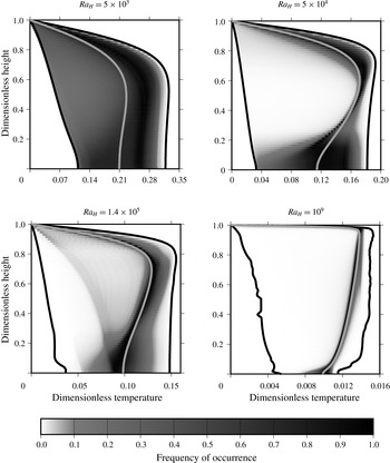
. Solid black lines correspond to the minimum and maximum temperatures recorded at each depth (‘cold’ and ‘hot’ temperature profiles), while solid light grey lines correspond to vertical profiles of the horizontally averaged temperature. Temperature values at each depth are shown on a white to black colour scale depending on their probability of occurrence. At
 $Ra_{H}=10^{9}$
, due to the overwhelming areal dominance of upwellings, the vertical profile of the most probable temperature is essentially identical to that of the horizontally averaged temperature.

4.1 Temperature distribution
The different regimes that have been observed are associated with different temperature distributions that reflect changes in the balance between downwellings and upwellings. Figure 6 illustrates how the horizontal temperature distribution varies with depth for four representative cases. In all cases, independently of the
 $Ra_{H}$
value, the spread of temperatures increases from zero at the top to a maximum at the base of the upper boundary layer, and then decreases towards the bottom of the fluid layer. This is due to internal heating, as shown by the steady increase of the minimum temperature with increasing depth (the cold profile in figure 6). In the steady-state hexagon regime at
 $Ra_{H}=5\times 10^{3}$
, temperatures are spread across the range due to the nearly equal areas occupied by upwellings and downwellings. In contrast, the temperature distribution in the spoke regime at
 $Ra_{H}=5\times 10^{4}$
is markedly peaked due to the large areas of upward return flow where lateral gradients are small (figure 5
b). ‘Peaked’ distributions are also a feature of time-dependent regimes, with a temperature range that decreases with increasing
 $Ra_{H}$
. In these cases, the flow can be described as a set of narrow downwellings going through nearly isothermal fluid. The gradual change from spread out to increasingly peaked distributions is interrupted in the sheet regime, as shown for
 $Ra_{H}=1.4\times 10^{5}$
in figure 6, which is yet another peculiarity of this regime.
4.2 Vertical distribution of the horizontally averaged temperature
One significant feature of convection in internally heated fluid layers is that the horizontally averaged temperature
 $T_{avg}$
decreases significantly with increasing depth below the upper boundary layer (figures 6 and 7). This is in marked contrast to Rayleigh–Bénard convection where the decrease of
 $T_{avg}$
only occurs for a narrow vertical extent at the base of the boundary layer. We find that the magnitude of the vertical gradient of
 $T_{avg}$
in the fluid interior decreases with increasing
 $Ra_{H}$
, as already noted by Parmentier & Sotin (Reference Parmentier and Sotin2000) and Moore (Reference Moore2008).
Horizontally averaged temperature profile obtained for two different values of the Rayleigh–Roberts number (
 $Ra_{H}$
) with either free slip (solid red lines) or rigid (solid black lines) boundary conditions.

Vertical profiles of the horizontally averaged temperature are shown in figure 7 for two values of
 $Ra_{H}$
(
 $10^{6}$
and
 $10^{8}$
) and for both types of boundary conditions. In all cases, the temperature at the bottom of the fluid is significantly smaller than at the base of the upper boundary layer, implying that the fluid interior is stably stratified. As
 $Ra_{H}$
increases, the vertical gradient of
 $T_{avg}$
at mid-depth decreases in parallel with the temperature contrast across the upper boundary layer. One notes again the important influence of the mechanical boundary conditions, which affect the magnitudes of both the temperature difference across the layer and the interior thermal gradient. They also imply different vertical temperature profiles in the lower parts of the fluid layer, where a sub-layer connects the stably stratified interior to the adiabatic lower boundary. There, rigid behaviour impedes the lateral spreading of cold fluid coming from downwellings, leading to a thicker sub-layer than in the free slip case. In order to characterize how the bulk thermal structure varies with the Rayleigh–Roberts number, we have determined the volume-averaged and basal temperatures, noted
 $T_{vol}$
and
 $T_{bot}$
, respectively, in all our numerical simulations. These results are reported in table 3 together with others that will be discussed in another section below.
Some characteristics of convection for the 45 numerical simulations carried out for this study.
 $T_{vol}k/Hd^{2}$
is the volume-averaged temperature and
 $T_{bot}k/Hd^{2}$
is the basal temperature. The other variables correspond to the average properties of downwellings at mid-depth:
 $A_{i}/d^{2}$
is the average horizontal cross-section,
 $\unicode[STIX]{x0394}T_{i}k/Hd^{2}$
is the average temperature contrast and
 $W_{i}d/\unicode[STIX]{x1D705}$
is the average vertical velocity. ‘NA’ indicates that it was not possible to obtain a reliable count of downwellings; ‘–’ indicates that no calculation was carried out.
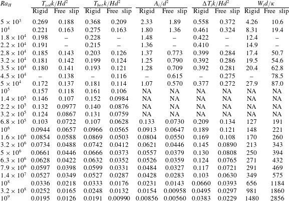
Dependence of (a) the volume-averaged temperature (
 $T_{vol}k/Hd^{2}$
) and (b) the horizontally averaged basal temperature (
 $T_{bot}k/Hd^{2}$
) as a function of the Rayleigh–Roberts number (
 $Ra_{H}$
). Results are shown for both free slip (red) and rigid (black) boundaries. Symbols indicate the convection planform that is achieved: a hexagonal pattern (square), a spoke pattern (star), a sheet regime (diamond) and the truncated hexagonal pattern (circle). Error bars, often smaller than the symbol size, indicate variations that are observed in time-dependent regimes. Solid lines are best fits to the data with power-law exponents set equal to
 $-1/4$
. Values for the various constants in the power-law relationships are listed in tables 4 and 5. Data with open symbols have not been included in the best-fit procedure.

Values of both
 $T_{vol}$
and
 $T_{bot}$
are shown as functions of the Rayleigh–Roberts number in figure 8 for all simulations. Overall, both temperatures decrease steadily with increasing
 $Ra_{H}$
with a marked change of trend for
 $Ra_{H}\approx 10^{5}$
, in conjunction with the occurrence of the sheet regime. For
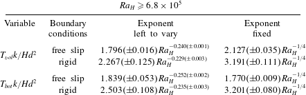
 $Ra_{H}\geqslant 6.8\times 10^{5}$
, the data appear to conform to power-law relationships with
 $Ra_{H}$
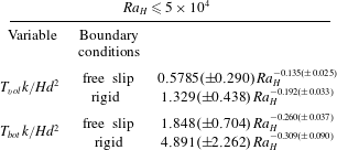
and best-fit parameter values are reported in table 4. The power-law exponents take values that are very close to
 $-1/4$
, which is the same value as that for the temperature contrast across the upper boundary layer. We thus surmise that
 $T_{vol}$
and
 $T_{bot}$
also scale as
 $Ra_{H}^{-1/4}$
and have implemented another best-fit procedure with the value of the power-law exponent set to
 $-1/4$
. As shown in table 4, this allows excellent fits to the data over a
 $Ra_{H}$
range spanning more than three orders of magnitude, with deviations that are typically less than
 $\pm 1\,\%$
. Results for the volume-averaged temperature are slightly less satisfactory for rigid boundaries but remain within
 $\pm 4\,\%$
of the simple
 $-1/4$
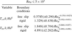
scaling law. For the sake of completeness, we have also determined best-fit power-law exponents for the steady-state regimes (table 5) but they do not account for the data very well as can be seen from the large errors.
4.3 Temperature fluctuations
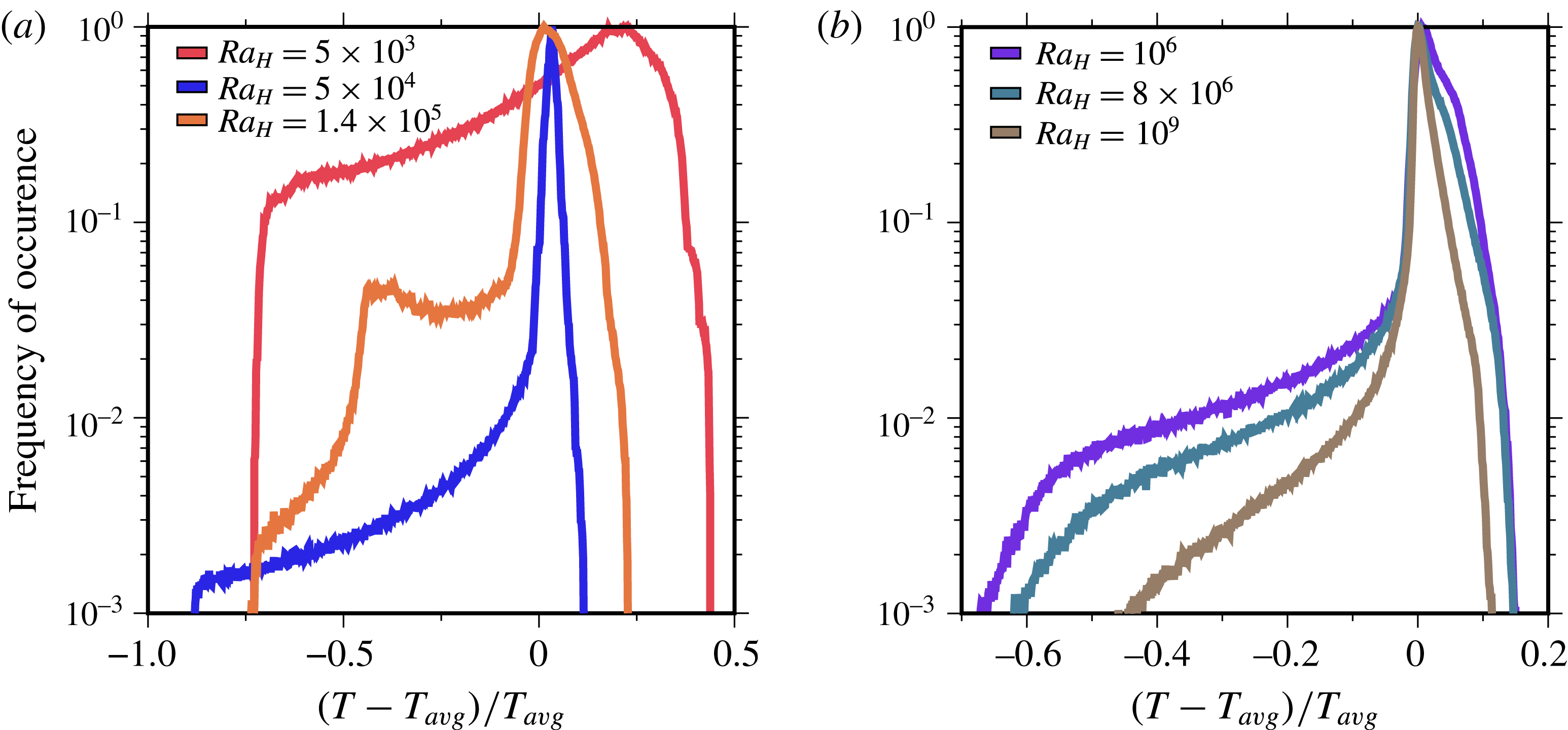
Temperature fluctuations at mid-depth in the layer are calculated as departures from the horizontal average at the same depth scaled to that average. Their distributions are strongly asymmetric, as shown in figure 9, in marked contrast to those of Rayleigh–Bénard convection, which are very close to being symmetrical (and Gaussian in the ‘soft turbulence’ regime, e.g. Castaing et al.
Reference Castaing, Gunaratne, Heslot, Kadanoff, Libchaber, Thomae, Wu, Zaleski and Zanetti1989). Their spread of values decreases as
 $Ra_{H}$
increases. In time-dependent regimes at large
 $Ra_{H}$
values (figure 9
b), they are markedly peaked with a slightly positive peak value that is due to the broad and rather homogeneous passive return flows that surround downgoing plumes. The distribution for the sheet regime stands out of all the others with its two peaks, corresponding to two well-separated populations for upwellings and downwellings (figure 9
a).
Parameters of best-fit power laws for the volume-averaged (
 $T_{vol}k/Hd^{2}$
) and basal (
 $T_{bot}k/Hd^{2}$
) temperatures for time-dependent regimes at large values of the Rayleigh–Roberts number (
 $Ra_{H}$
). Results in the right-hand column have been obtained by setting the power-law exponents to
 $-1/4$
.
Parameters of empirical best-fit power laws for the volume-averaged (
 $T_{vol}k/Hd^{2}$
) and basal (
 $T_{bot}k/Hd^{2}$
) temperatures in steady-state regimes at low values of the Rayleigh–Roberts number (
 $Ra_{H}$
).
Distribution of the dimensionless time-averaged temperature fluctuation
 $\unicode[STIX]{x1D703}/T_{avg}=(T-T_{avg})/T_{avg}$
in the fluid layer at mid-depth (
 $z=0.5$
) for (a) moderate values and (b) large values of the Rayleigh–Roberts number (
 $Ra_{H}$
) with free slip boundaries at the top and bottom. Distributions for time-dependent regimes are obtained by stacking a large number of instantaneous ones.

5 The characteristics of downwellings
In an internally heated fluid layer, downwellings occur as discrete entities associated with large deviations from the horizontally averaged temperature. We therefore focus on them to describe convection and determine some of their characteristics, such as the average number per unit area, the horizontal cross-section, the average temperature and the vertical velocity. As discussed above, convective planforms may change with increasing depth below the boundary layer and we shall restrict our analysis to structures at mid-depth in the fluid interior, away from the upper thermal boundary layer. Results for the two types of boundary conditions are qualitatively similar and we restrict the discussion to free slip cases for the sake of simplicity.
5.1 Detection method
In order to deal with the very large number of results, we have sought for an automatic procedure to detect downwellings and to determine their lateral dimensions. The number of downwellings and their average characteristics vary slightly with time in time-dependent regimes, suggesting that our finite computational domains do not allow a comprehensive statistical sampling of all the possible flow configurations. Steady average properties could be obtained by enlarging the computational domain, which would thus host a larger number of downwellings. An alternative strategy is to average results obtained at different times. Because our calculations are time-dependent, the latter is easier to implement and was therefore adopted.
Several methods have been used to detect downwellings and upwellings in convective systems. Most of these have relied on the temperature field, including the definition of a threshold value that separates an individual plume from the background (Labrosse Reference Labrosse2002; Zhong Reference Zhong2005; Galsa & Lenkey Reference Galsa and Lenkey2007; Zhou & Xia Reference Zhou and Xia2010). Others have used the convective heat flux, the local dissipation rate or the conditional average of the velocity on the temperature (Ching et al. Reference Ching, Guo, Shang, Tong and Xia2004; Shishkina & Wagner Reference Shishkina and Wagner2008). The latter, more elaborate, methods were devised to identify coherent structures in the complex temperature fields of turbulent Rayleigh–Bénard convection. In our study, flow is in a laminar regime and downwellings clearly stand out of the background temperature field so that the former, and simpler, method was sufficient.
We expect that downwellings, which are driven by a downward buoyancy force, are associated with negative temperature anomalies. In time-dependent regimes, however, one observes tiny areas with very small negative anomalies that are not part of coherent structures and that are highly transient. In order to exclude these small anomalies, we introduce a threshold temperature
 $T_{ref}$
, related to a ‘detection parameter’
 $p_{c}$
,
 $$\begin{eqnarray}\displaystyle & \displaystyle {\displaystyle \frac{T_{ref}-T_{avg}}{T_{avg}}}=-p_{c} & \displaystyle\end{eqnarray}$$
so that fluctuations at any depth are properly scaled to the local temperature field. Obviously, the temperature threshold decreases with increasing
 $p_{c}$
. As described above, at some distance of the unstable boundary layer, downwellings take the shapes of laminar plumes with nearly cylindrical outlines, where temperature decreases to a minimum value at the downwelling centre. Viewed in a horizontal cross-section, a plume thus appears as an area where temperature varies radially in a systematic manner. For each threshold temperature value, we have determined contour lines that close upon themselves. With increasing
 $p_{c}$
, the procedure selects parts of the plumes that are increasingly colder, such that it hits the same plume over increasingly smaller areas. Eventually, of course, the temperature threshold decreases below the smallest downwelling temperature and the procedure returns a count of zero. This method is not efficient for the sheet regime due to the contorted structures and their complex temperature fields, and hence was not used in this regime.
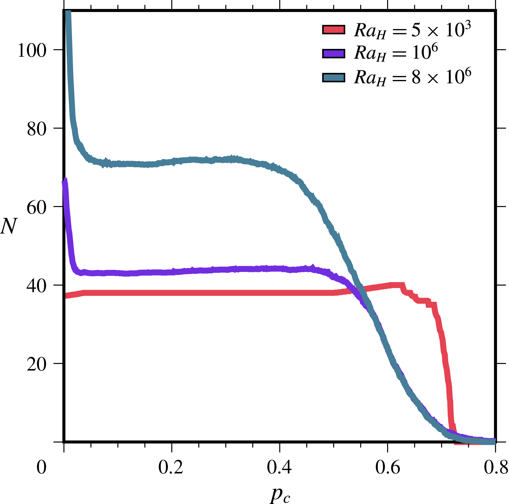
Figure 10 shows the number of structures that are hit as a function of the detection parameter. In the steady-state regime at
 $Ra_{H}=5\times 10^{3}$
, temperature varies smoothly in the horizontal plane in a well-defined periodic pattern and negative temperature fluctuations are always found in coherent structures. In this case, the number of ‘hits’ is constant for
 $0\leqslant p_{c}\leqslant 0.6$
and drops down sharply for
 $p_{c}\gtrsim 0.7$
, which corresponds to the coldest temperature. Results are more complicated for time-dependent regimes (figure 10). The number of hits decreases rapidly for small values of the detection parameter and stabilizes to an almost constant value over a large range of
 $p_{c}$
values, typically from close to 0 to 0.4–0.5. The initial decrease is due to the tiny areas with small negative anomalies that have been mentioned above, because a large proportion of these small anomalies are detected for very small values of the detection parameter. In contrast, the
 $p_{c}$
‘plateau’ is due to coherent structures that, as explained above, are expected to be detected over a finite
 $p_{c}$
interval. The number of hits starts to decrease above a certain
 $p_{c}$
value more gradually than in steady-state regimes, due to the more heterogeneous temperature fields.
Number of structures with negative thermal anomalies (
 $N$
) detected as a function of detection parameter
 $p_{c}$
for a horizontal plane located at mid-depth (
 $z=0.5$
) in a layer with free slip boundaries. Downwellings are identified using the algorithm described in the text. In this figure,
 $N$
is not scaled to the horizontal area in order to show the total number of hits and its variation as a function of
 $p_{c}$
. Results are shown for different values of the Rayleigh–Roberts number
 $Ra_{H}$
. Note the difference between the steady-state regime at
 $Ra_{H}=5\times 10^{3}$
and the two time-dependent ones at larger values of
 $Ra_{H}$
.

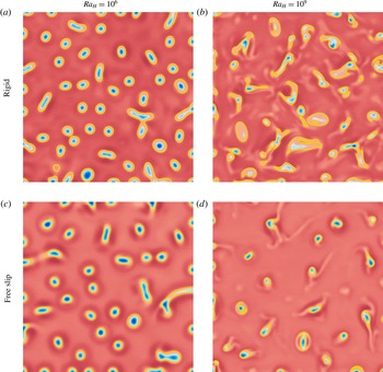
Temperature field for rigid (a,b) and free slip (c,d) boundaries in a plane located at mid-depth for
 $Ra_{H}=10^{6}$
(a,c) and
 $10^{9}$
(b,d). Results for
 $Ra_{H}=10^{9}$
are only shown in part of the horizontal plane, over a dimensionless 2 : 2 square, in order to facilitate visualization. Note that the dimension of the horizontal plane is different for
 $Ra_{H}=10^{6}$
(6 : 6) and
 $10^{9}$
(2 : 2). Blue and red colours correspond to material that is colder and hotter than the local horizontal average, respectively. The colour scale is not the same in all panels and was chosen to enhance convective structures. Yellow contours illustrate the downwelling outlines that have been determined using the detection procedure described in the text. Values of the detection parameter
 $p_{c}$
were 0.12 and 0.03 for cases with free slip and rigid boundaries, respectively (see text). The numerical resolution and domain aspect ratio are not the same for all these calculations (see table 1) and were changed to deal with the decreasing size of convective cells.

The performance of the detection procedure is illustrated in figure 11, which shows the temperature field at mid-depth for two time-dependent regimes and for both free slip and rigid boundaries. Downwellings appear as coherent structures with well-defined radial distributions of negative temperature values. They have predominantly circular outlines at
 $Ra_{H}=10^{6}$
and more complex and contorted ones at
 $Ra_{H}=10^{9}$
. One notes that, away from the downwellings, the background temperature field is smooth for
 $Ra_{H}=10^{6}$
and rugged for
 $Ra_{H}=10^{9}$
. In the latter case, the temperature field is heterogeneous and includes downwellings of different strengths, i.e. characterized by different temperature anomalies. A few downwellings have detached from the upper boundary layer and leave faint ‘ghost’ thermal traces that are picked up by the detection procedure at small
 $p_{c}$
values (figure 10). These must not be included in the tally of downwellings, which is easily achieved by raising the detection threshold. A snapshot at a randomly chosen time may not capture a fully representative temperature field and we have repeated the tally several times. Deviations about the mean are small and will be shown.
Our goal is to obtain robust results for all numerical simulations such that they can be compared to one another. We therefore need to follow the same procedure for each calculation in order to avoid potential artefacts due to changing criteria. In other words, we have to consider the same detection parameter
 $p_{c}$
for each set of numerical simulations, and to do so we proceed as follows. Steady-state regimes are straightforward with stable counts even for very small values of the detection parameter. For time-dependent regimes, close inspection of the number of hits shows that there is a local minimum at the lower end of the
 $p_{c}$
plateau (figure 10). This can be understood from figure 11, where it may be seen that the temperature has more than a single local minimum in a few downwellings with contorted outlines. Such structures would be counted as one at very low
 $p_{c}$
values and as two, and sometimes three, at slightly higher
 $p_{c}$
values. We conclude that the most appropriate choice is the first local minimum in the number of hits. The uncertainty is very small because the number of counts in the intermediate
 $p_{c}$
range does not change by more than two or three units out of a few tens. A constant value of
 $p_{c}=0.12$
is appropriate for free slip boundaries at all
 $Ra_{H}$
values. Detection levels are different for cases with rigid boundaries owing to the different downwelling pattern and an appropriate choice is
 $p_{c}=0.03$
. Figure 11 shows the downwellings that have been identified by this procedure as well as their outlines (which appear as yellow contours).
5.2 Data
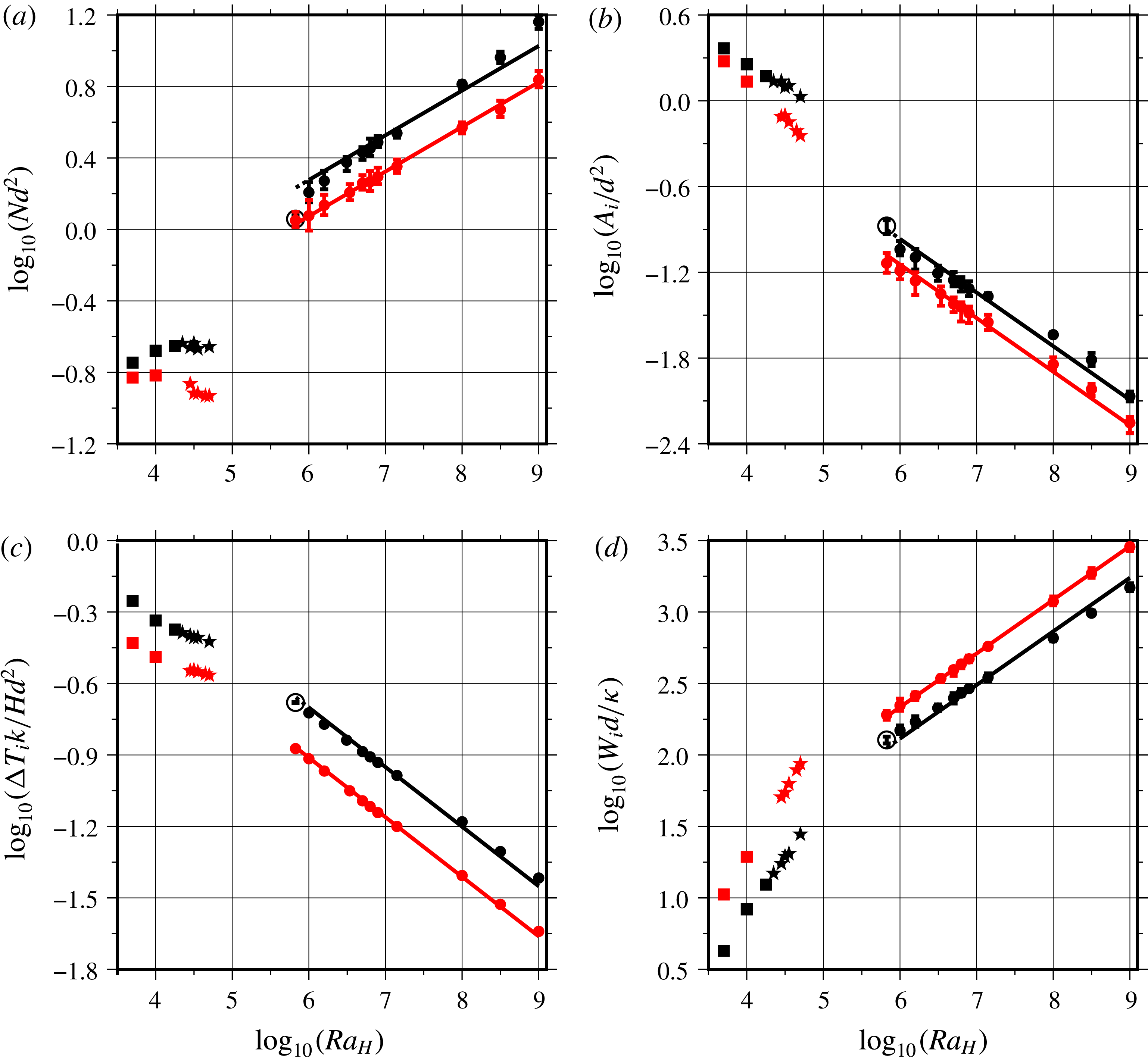
With the method that has just been described, we were able to analyse a large number of calculations with minimum effort. We have determined the values of four different variables at mid-depth in the layer: the number of downwellings per unit area, which allows calculation of the average area of a convection cell made of a downwelling and its associated return flow, the average areal extent of the negative thermal anomalies
 $A_{i}$
, the average thermal anomaly,
 $\unicode[STIX]{x0394}T_{i}$
, and the average vertical velocity,
 $W_{i}$
. Values are made dimensionless using
 $d^{2}$
as a scale for area,
 $Hd^{2}/k$
as temperature scale and
 $\unicode[STIX]{x1D705}/d$
as velocity scale.
Figure 12 shows results for all calculations save those for the sheet regime in the intermediate
 $Ra_{H}$
range. Data for steady-state regimes at
 $Ra_{H}\leqslant 5\times 10^{4}$
and time-dependent ones at
 $Ra_{H}\geqslant 6.8\times 10^{5}$
clearly define two different sets of relationships as a function of
 $Ra_{H}$
. The most significant difference lies in the number of downwellings per unit area, which remains approximately constant in steady-state cases in contrast to time-dependent ones. Thus, the characteristic spacing between downwellings scales with the total layer thickness for the former and not for the latter. This fundamental change of convection characteristics does not occur as a bifurcation at some threshold
 $Ra_{H}$
value but is achieved in the transitional sheet regime over a range of Rayleigh–Roberts numbers. All other variables vary monotonically as
 $Ra_{H}$
increases in both steady-state and time-dependent cases. The size of downwellings, as measured by the areal extent of the thermal anomaly, decreases markedly as
 $Ra_{H}$
increases whilst velocity values increase. Data for the two types of boundary conditions exhibit parallel trends but differ by significant factors. For example, the magnitude of thermal anomalies is 35 % larger for rigid boundaries than for free slip ones. The greatest difference is in the number of downwellings in time-dependent cases, which is larger by 60 % in rigid cases.
Dependence of (a) the number of downwellings per unit area (
 $Nd^{2}$
), (b) their average horizontal cross-section (
 $A_{i}/d^{2}$
), (c) their average temperature contrast (
 $\unicode[STIX]{x0394}T_{i}k/Hd^{2}$
), (d) their average vertical velocity (
 $W_{i}d/\unicode[STIX]{x1D705}$
) at mid-depth in the fluid layer as a function of the Rayleigh–Roberts number (
 $Ra_{H}$
). Results are shown for both free slip (red) and rigid (black) boundaries. Downwellings are identified and contoured using an automatic procedure described in the text. Different symbols indicate the convection pattern stable at a given
 $Ra_{H}$
: a hexagonal pattern (square), a spoke pattern (star) and the truncated hexagonal pattern (circle). Error bars, often smaller than the symbol size, indicate variations that are observed in time-dependent regimes. Solid lines are best fits to the data with power laws predicted by the scaling analysis of § 5.3. Values for the various constants in the power-law relationships are listed in tables 6 and 7. Data with open symbols have not been included in the best-fit procedure.

In order to facilitate comparisons and to evaluate the sensitivity of the variables to
 $Ra_{H}$
, we have determined power-law relationships using a best-fit procedure, such that:
 $$\begin{eqnarray}\displaystyle & \displaystyle N=C_{N}(1/d^{2})Ra_{H}^{\unicode[STIX]{x1D6FD}_{N}}, & \displaystyle\end{eqnarray}$$
 $$\begin{eqnarray}\displaystyle & \displaystyle A_{i}=C_{A}d^{2}Ra_{H}^{\unicode[STIX]{x1D6FD}_{A}}, & \displaystyle\end{eqnarray}$$
 $$\begin{eqnarray}\displaystyle & \displaystyle \unicode[STIX]{x0394}T_{i}=C_{T}(Hd^{2}/k)Ra_{H}^{\unicode[STIX]{x1D6FD}_{T}}, & \displaystyle\end{eqnarray}$$
 $$\begin{eqnarray}\displaystyle & \displaystyle W_{i}=C_{W}(\unicode[STIX]{x1D705}/d)Ra_{H}^{\unicode[STIX]{x1D6FD}_{W}}, & \displaystyle\end{eqnarray}$$
where
 $C_{N}$
,
 $C_{A}$
,
 $C_{T}$
and
 $C_{W}$
are dimensionless proportionality constants and where
 $\unicode[STIX]{x1D6FD}_{N}$
,
 $\unicode[STIX]{x1D6FD}_{A}$
,
 $\unicode[STIX]{x1D6FD}_{T}$
and
 $\unicode[STIX]{x1D6FD}_{W}$
are power-law exponents. Since variables do not follow the same trends for
 $Ra_{H}\leqslant 5\times 10^{4}$
and for
 $Ra_{H}\geqslant 6.8\times 10^{5}$
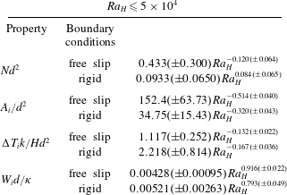
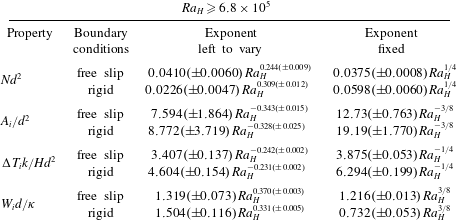
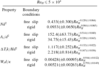
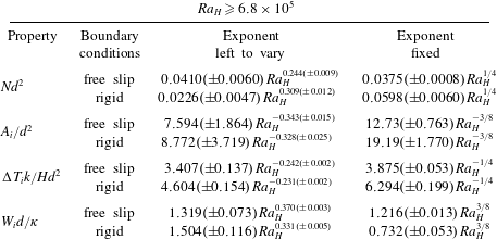
(figure 12), we have determined two sets of parameters which are listed in tables 6 and 7. Overall, power-law relationships allow very good fits to the numerical results for steady-state regimes and an excellent fit for time-dependent regimes. The contrasting exponents for steady-state and time-dependent cases confirm the fundamental difference of convection characteristics between the two. Limitations of a best-fit procedure where both the proportionality constant and the exponent are left to vary are well known. Variations of the exponent can be balanced by changes of the proportionality coefficient, which is likely to induce large uncertainties on both parameters. In the next section, we use simple scaling arguments to derive values for the various exponents and compare them to the numerical results.
Parameters of empirical best-fit power laws for the characteristics of downwellings in a planform located at mid-depth for steady-state regimes at low values of the Rayleigh–Roberts number (
 $Ra_{H}$
).
Parameters of best-fit power laws for the characteristics of downwellings in a planform located at mid-depth for time-dependent regimes at large values of the Rayleigh–Roberts number (
 $Ra_{H}$
). Results in the right-hand column have been obtained by setting exponents to values derived from scaling arguments (see text).
5.3 Scaling analysis
We restrict the analysis to time-dependent regimes which are such that the dynamics of the upper boundary layer is independent of the total fluid thickness (Vilella & Kaminski Reference Vilella and Kaminski2017). In this case, the boundary layer thickness and the temperature contrast across it can be derived from local scaling arguments (table 2). We argue that the interior temperature anomaly
 $\unicode[STIX]{x0394}T_{i}$
scales with
 $\unicode[STIX]{x0394}T_{TBL}$
the temperature contrast across the upper boundary layer, which is such that
 $\unicode[STIX]{x0394}T_{TBL}\sim (Hd^{2}/k)Ra_{H}^{-1/4}$
(3.1). This implies that
 $\unicode[STIX]{x1D6FD}_{T}=-1/4$
, which is close to the empirically derived values (table 7, figure 12
c). Setting
 $\unicode[STIX]{x1D6FD}_{T}=-1/4$
, we find that the numerical data for both free slip and rigid boundaries are within a few per cent of the best-fit relationships. Interestingly, the proportionality coefficients in the scaling relationships for
 $\unicode[STIX]{x0394}T_{i}$
and
 $\unicode[STIX]{x0394}T_{TBL}$
increase by almost the same factor when one moves from free slip boundaries to rigid ones, which confirms that it is indeed the temperature contrast across the boundary layer that sets the amplitude of thermal anomalies in the fluid interior.
In order to derive values for the other power-law exponents, we take into account the structure of the flow field. For
 $10^{6}\leqslant Ra_{H}\lesssim 10^{8}$
, the flow field may be described as a set of downwellings that go through the whole fluid layer and show up as isolated negative thermal anomalies in an almost uniform background. Such a simple description may not capture all the complex structures that are observed at the largest values of
 $Ra_{H}$
and we shall evaluate its relevance a posteriori. We thus consider that each downwelling draws fluid from the upper boundary layer over an area
 $\unicode[STIX]{x0394}S$
and, on average, transports heat at a rate which is equal to
 $$\begin{eqnarray}\displaystyle & \displaystyle Q=q\unicode[STIX]{x0394}S=Hd\unicode[STIX]{x0394}S, & \displaystyle\end{eqnarray}$$
where
 $q=Hd$
is the heat flux through the top surface.
 $\unicode[STIX]{x0394}S$
is inversely proportional to the number of downwellings per unit area, therefore
 $$\begin{eqnarray}\displaystyle & \displaystyle Q\sim {\displaystyle \frac{Hd}{N}}. & \displaystyle\end{eqnarray}$$
Downwellings are defined by their average thermal contrast with respect to the average background temperature,
 $\unicode[STIX]{x0394}T_{i}$
. They develop circular cross-sections
 $A_{i}$
below the upper boundary layer, with radius
 $R$
, such that
 $R^{2}\sim A_{i}$
. The associated velocity scale is
 $$\begin{eqnarray}\displaystyle & \displaystyle W_{i}\sim {\displaystyle \frac{\unicode[STIX]{x1D70C}g\unicode[STIX]{x1D6FC}\unicode[STIX]{x0394}T_{i}R^{2}}{\unicode[STIX]{x1D702}}}. & \displaystyle\end{eqnarray}$$
Conservation of the energy flux implies that
 $$\begin{eqnarray}\displaystyle & \displaystyle Q\sim \unicode[STIX]{x1D70C}C_{p}W_{i}\unicode[STIX]{x0394}T_{i}R^{2}, & \displaystyle\end{eqnarray}$$
where
 $C_{p}$
is heat capacity. Combining (5.8) and (5.9), one obtains
 $$\begin{eqnarray}\displaystyle & \displaystyle W_{i}\sim \left({\displaystyle \frac{\unicode[STIX]{x1D705}\unicode[STIX]{x1D70C}g\unicode[STIX]{x1D6FC}Q}{\unicode[STIX]{x1D702}k}}\right)^{1/2}, & \displaystyle\end{eqnarray}$$
the Stokes velocity scale for a laminar plume (Batchelor Reference Batchelor1954), which is an appropriate scale for the transient plumes generated in time-dependent regimes (Kaminski & Jaupart Reference Kaminski and Jaupart2003). We note that this scale depends explicitly on neither the temperature anomaly nor the plume cross-section. Substituting (5.7) in the velocity scale (5.10) together with the Rayleigh–Roberts number (1.1) and power-law expressions for
 $N$
(5.2) and
 $W_{i}$
(5.5), we obtain
 $$\begin{eqnarray}\displaystyle & \displaystyle 2\unicode[STIX]{x1D6FD}_{W}=1-\unicode[STIX]{x1D6FD}_{N}. & \displaystyle\end{eqnarray}$$
Within uncertainty, the empirical exponents of table 7 are fully consistent with this relationship. For free slip cases, for example,
 $\unicode[STIX]{x1D6FD}_{W}\approx 0.370$
and
 $\unicode[STIX]{x1D6FD}_{N}\approx 0.244$
. Similarly, substituting for (5.7) in (5.9), we obtain
 $$\begin{eqnarray}\displaystyle 0=\unicode[STIX]{x1D6FD}_{N}+\unicode[STIX]{x1D6FD}_{A}+\unicode[STIX]{x1D6FD}_{T}+\unicode[STIX]{x1D6FD}_{W}, & & \displaystyle\end{eqnarray}$$
which is also consistent with the empirically derived exponents and their uncertainties (table 7).
In a laminar regime, the radius of the downwelling is set by a balance between vertical heat advection and horizontal diffusion, such that
 $$\begin{eqnarray}\displaystyle & \displaystyle R\sim \left({\displaystyle \frac{\unicode[STIX]{x1D705}z}{W_{i}}}\right)^{1/2}, & \displaystyle\end{eqnarray}$$
where
 $z$
is the distance from source, taken here as the distance to the upper boundary. We determine the velocity at mid-depth, i.e. at a fixed distance equal to
 $d/2$
, implying that
 $R\sim (\unicode[STIX]{x1D705}d/W_{i})^{1/2}$
and hence that
 $A_{i}\sim R^{2}\sim \unicode[STIX]{x1D705}d/W_{i}$
. This implies in turn that
 $$\begin{eqnarray}\displaystyle & \displaystyle \unicode[STIX]{x1D6FD}_{A}=-\unicode[STIX]{x1D6FD}_{W}. & \displaystyle\end{eqnarray}$$
This is again consistent with the data in table 7 and their uncertainties. Using (5.12), one deduces further that
 $\unicode[STIX]{x1D6FD}_{T}=-\unicode[STIX]{x1D6FD}_{N}$
. This is also verified, albeit less satisfactorily for rigid boundaries than for free slip ones. We shall come back to this point at the end of this section.
The above relationships between the four power-law exponents are all consistent with the empirical best-fit values, which supports the validity of the physical arguments. Substituting for the value of
 $\unicode[STIX]{x1D6FD}_{T}$
(
 $-1/4$
), we find that
 $\unicode[STIX]{x1D6FD}_{W}=3/8$
,
 $\unicode[STIX]{x1D6FD}_{A}=-3/8$
and
 $\unicode[STIX]{x1D6FD}_{N}=1/4$
. These exponents allow excellent fits to the numerical data with few exceptions (figure 12). All the data are typically within less than
 $\pm 2\,\%$
of the best-fit power laws for free slip boundaries (except for
 $A_{i}$
where the maximum deviation rises to
 $\pm 6\,\%$
), but results are slightly less satisfactory for rigid boundaries (table 7). Departures from the proposed scalings may be attributed to two factors. One is due to the assumption that the downwellings issue from point sources, whereas they emanate from a boundary layer of finite thickness. This problem is more severe for rigid boundary cases due to their thicker boundary layers. Another factor is that the shapes of the downwellings are not as regular in cross-section as we have assumed, as shown by figure 5. This is most pronounced for flows between rigid boundaries at large
 $Ra_{H}$
values (figure 11) but, even in these cases, this only degrades significantly the quality of the fits to velocity values and to the number of plumes (table 7). Nevertheless, the power laws for these two variables remain accurate to within
 $\pm 10\,\%$
over the whole range of Rayleigh–Roberts number investigated.
5.4 Comparison with previous studies
The above results and scaling laws have few equivalents in previous studies. The number of downwellings was determined by Parmentier & Sotin (Reference Parmentier and Sotin2000) for free slip boundaries. Their values are consistent with the same
 $Ra_{H}^{1/4}$
scaling law but are somewhat larger than ours (by approximately 30 %). This difference may be attributed to the smaller aspect ratio of their computation domain, which was equal to either 2 or 1. We have found indeed that the number of downwellings increases slightly but systematically as the aspect ratio is decreased and argue that this is due to the preferential generation of downwellings at the walls and corners of the domain (supplementary material). In fact, there can be little doubt that the results of Parmentier & Sotin (Reference Parmentier and Sotin2000) bear the influence of the vertical bounding walls: for the same Rayleigh–Roberts number (
 $Ra_{H}=10^{8}$
), the value of
 $Nd^{2}$
changes when lateral boundary conditions are switched from reflecting to periodic.
At large values of
 $Ra_{H}$
, the downwellings are generated in a thin upper boundary layer, much as those of Rayleigh–Bénard (RB) convection, and it is worthwhile to compare the two cases. The latter type of convection is controlled by the Rayleigh number, which is defined as
 $$\begin{eqnarray}\displaystyle & \displaystyle Ra={\displaystyle \frac{\unicode[STIX]{x1D70C}g\unicode[STIX]{x1D6FC}\unicode[STIX]{x0394}T^{\ast }d^{3}}{\unicode[STIX]{x1D702}\unicode[STIX]{x1D705}}}, & \displaystyle\end{eqnarray}$$
where
 $\unicode[STIX]{x0394}T^{\ast }$
is the temperature difference across the layer and where all the other variables are identical to those of this paper. In high-resolution numerical simulations of RB convection, Zhong (Reference Zhong2005) found that the number of downwellings increases approximately with
 $Ra^{1/3}$
over a limited range of Rayleigh numbers and seems to level off for Rayleigh numbers larger than approximately
 $10^{8}$
. The former behaviour is reminiscent of that of this paper but the latter is not: as shown by figure 12, the number of downwellings increases steadily over the whole
 $Ra_{H}$
range investigated. We note that the same behaviour was observed by Parmentier & Sotin (Reference Parmentier and Sotin2000) over the same
 $Ra_{H}$
range with a completely different numerical method. One might expect that the number of downwellings cannot increase indefinitely due to a ‘crowding’ effect, but, in this aspect, there is a major difference between basal heated and internally heated convection. The former has both active upwellings and downwellings competing for space in contrast to the latter, which only involves active downwellings. Thus, it may well be that crowding limitations in internally heated convective fluids become important at values of the Rayleigh–Roberts number that are larger than those of this paper. One might remark, however, that the fractional area of downwellings scales as
 $NA_{i}\sim Ra_{H}^{-1/8}$
(table 7), which decreases with increasing
 $Ra_{H}$
.
6 Discussion and implications for convection in planetary bodies
6.1 General features of internally heated convection
Our numerical simulations illustrate the important effect of boundary conditions on the downwelling characteristics: for a given regime and hence a given Rayleigh–Roberts number, downwellings are significantly colder, narrower and wider apart beneath free slip boundaries than beneath rigid ones. With the four scaling laws that have been derived here and adding those for the thickness and temperature difference across the upper thermal boundary layer (3.1) as well as those for the volume-averaged and bottom temperatures, one can determine all the key characteristics of time-dependent convection from knowledge of the
 $Ra_{H}$
value. For geophysical/planetological applications, however, this may not be manageable, partly because calculation of the Rayleigh–Roberts number is fraught with many uncertainties and partly because other factors come into play, such as large variations of physical properties as a function of temperature and pressure and the presence of continents and oceans at the Earth’s surface. It may be more useful, therefore, to adopt a different perspective; all the variables of interest here form a self-consistent set, such that knowledge of any one of them leads to estimates for all the others.
In rocky planets with a solid mantle, it is easier to obtain information on the upper boundary layer structure than on the deeper flow characteristics. With respect to a Rayleigh–Bénard set-up, internal heat sources imply a different relationship between downwellings in the fluid interior and the unstable boundary layer at the top. In Rayleigh–Bénard convection, a fixed temperature difference is maintained across the fluid layer, which leads to the formation of boundary layers at both the top and bottom and to upwellings and downwellings of similar strength. We have briefly commented on the different temperature distributions that are generated by the two types of convection. In laminar Rayleigh–Bénard convection at high values of
 $Ra$
(
 ${\gtrsim}10^{5}$
), the average downwelling velocity
 $W_{RB}$
and the boundary layer thickness
 $\unicode[STIX]{x1D6FF}_{RB}$
scale as
 $(\unicode[STIX]{x1D705}/d)Ra^{2/3}$
and
 $dRa^{-1/3}$
, respectively (Turcotte & Oxburgh Reference Turcotte and Oxburgh1967; Galsa & Lenkey Reference Galsa and Lenkey2007). Note that these relationships may not be valid for
 $Ra$
values that are larger than about
 $10^{7}$
(e.g. Zhong Reference Zhong2005). One deduces that
 $$\begin{eqnarray}\displaystyle & \displaystyle W_{RB}\sim {\displaystyle \frac{\unicode[STIX]{x1D705}}{d}}\left({\displaystyle \frac{\unicode[STIX]{x1D6FF}_{RB}}{d}}\right)^{-2}. & \displaystyle\end{eqnarray}$$
In an internally heated convecting layer, combining the scaling laws derived above with (3.1) for the boundary layer thickness, we obtain
 $$\begin{eqnarray}\displaystyle & \displaystyle W_{i}\sim {\displaystyle \frac{\unicode[STIX]{x1D705}}{d}}\left({\displaystyle \frac{\unicode[STIX]{x1D6FF}}{d}}\right)^{-3/2}. & \displaystyle\end{eqnarray}$$
Alternatively, one could derive relationships between velocity and the temperature difference across the boundary layer because it may be easier to obtain constraints on temperature than on thickness in some cases. The key point, however, is the same: the relationship between downwellings and boundary layer structure is fundamentally different for Rayleigh–Bénard and internally heated systems.
6.2 Subduction zones on Earth
The Earth’s mantle is clearly more complex than the internally heated fluid layer studied here. Nevertheless, it is worth evaluating our results in this context because they illustrate the peculiarities of internally heated systems and the range of dynamical regimes that can be achieved. Our point is not to claim that our calculations provide realistic representations of the Earth’s mantle but to argue that one should be careful when attributing Earth’s characteristic features to a particular mechanism.
The Earth’s present-day convective regime is characterized by a small number of ‘plates’ created at mid-ocean ridges and subducted along trenches that stretch over large horizontal distances. Surprising features are the large range of plate dimensions and velocities, which typically span approximately one order of magnitude, and the complex network of subduction zones which do not conform to any simple geometrical pattern (Mora et al. Reference Mora, Seton, Quevedo and Müller2013). Seismic images of the mantle interior show that mid-ocean ridges, which are the surface expressions of local upwellings, are not underlain by deep-seated thermal anomalies, in marked contrast to subduction zones (e.g. Ritsema et al. Reference Ritsema, Deuss, Van Heijst and Woodhouse2011). Such characteristics are hallmarks of an internally heated convective system. Seismological data also indicate that subducting plates remain whole as they go through the upper mantle. In this regard, the sheet regime is of special interest because of its large-scale irregular network of narrow linear downwellings that extend to the base of the layer. The most challenging fact is probably that Earth seems to be the only rocky planet of the solar system hosting plate tectonics. Planet Venus, which is comparable in size and composition, has a convective mantle, as shown by the many volcanoes that dot its surface, but no plates and no subduction zones (Schubert et al. Reference Schubert, Hussmann, Lainey, Matson, McKinnon, Sohl, Sotin, Tobie, Turrini and Van Hoolst2010). Another conundrum deals with when plate tectonics started on Earth, which remains hotly debated today. Some authors have proposed that plate tectonics is essentially as old as the planet and others have argued that its onset coincided with a major compositional change that occurred 3 Gyr ago in the subcontinental lithospheric mantle (Shirey & Richardson Reference Shirey and Richardson2011). Answers to both questions may be sought in transient evolutionary models, such that plate tectonics is only active for a finite length of time. As a planet cools down and its heat sources get depleted, the Rayleigh–Roberts decreases and the convection regime and planform are bound to change. The sheet regime serves to emphasize the dramatic planform transformations that can occur.
Subducting slabs can be linked to the downgoing sheets that have been documented here. Subduction zones occasionally form triple junctions, such as in the Boso subduction margin, central Japan (Yujiro et al.
Reference Yujiro, Tetsuzo, Hinako, Hidekazu, Kantaro and Hidetsugu1989), which are strongly reminiscent of the planforms of this study. Our calculations show that sheets are not the only form of convection that can occur and that they require values of the Rayleigh–Roberts number above a certain threshold. Planets with small
 $Ra_{H}$
values, due either to their small sizes or to their small rates of internal heat production, are not expected to be in the same regime and would likely involve hexagons with an axial upwelling. By the same token, the fact that the downgoing sheets of Earth remain whole over the total vertical extent of the upper mantle provides another constraint: sheets break up into nearly cylindrical downgoing plumes if the Rayleigh–Roberts number exceeds a critical value. Thus, plate tectonics, which is the current convection regime on Earth, may not be the standard regime for all silicate planets and, furthermore, may not have prevailed early in Earth’s history, as suggested by Jellinek & Jackson (Reference Jellinek and Jackson2015) amongst others. One should also note that the sheet regime exists over a much larger range of
 $Ra_{H}$
values for rigid boundaries than for free ones, which illustrates the sensitivity of the superficial convection planform and the bulk flow characteristics to the mechanical boundary condition at the top.
7 Conclusion
Three-dimensional numerical simulations of laminar convection in an internally heated fluid layer cooled from above, illustrate the different superficial planforms that may be generated. As the Rayleigh–Roberts number increases, we have found four different planforms described as hexagons with an axial cylindrical downwelling, hexagons with a spoke-like axial downwelling, networks of linear downwellings or sheets and finally truncated hexagons. Rigid and free slip boundaries allow the same planforms but are associated with marked differences in the spacing and other characteristics of convective motions. In time-dependent regimes at large
 $Ra_{H}$
values (
 ${\geqslant}10^{6}$
), complex superficial planforms morph into arrays of nearly equally spaced cylindrical plume-like downwellings with characteristics that depend on the
 $Ra_{H}$
value in systematic ways. Temperature distributions in both the horizontal and vertical directions are markedly different from those of Rayleigh–Bénard convection. Scaling laws for the main variables of interest, including the thermal anomalies, velocities, dimensions and spacing of descending plumes, have been developed and are fully consistent with numerical results over a
 $Ra_{H}$
range spanning three orders of magnitude. They illustrate important differences of boundary layer dynamics with respect to Rayleigh–Bénard convection.
The sheet regime deserves more attention because of its peculiar characteristics and also because it illustrates that dramatic reorganizations of flow structure in rocky planets can be caused by small changes of internal heat release and physical properties. Much is likely to be gained by investigating how such reorganizations proceed and how sensitive they are to temperature-dependent fluid properties.
Acknowledgements
We thank three anonymous reviewers for their thorough and constructive comments that helped us to produce a much improved paper. We also thank J. Wettlaufer for his editorial handling of the manuscript. This work was funded by the ANR-11-IS04-0004 project and supported by the Tellus/PNP program of INSU-CNRS. Numerical computations were performed on the S-CAPAD platform, IPGP, France and using HPC resources from GENCI-IDRIS (Grant 2013-047033).
Supplementary material
Supplementary material is available at https://doi.org/10.1017/jfm.2018.316.