1. Introduction
Acoustic-gravity waves are mechanical waves in compressible fluids in a gravity field. These waves play an important role in the dynamics of stars and planetary atmospheres (Duvall et al. Reference Duvall, Jefferies, Harvey and Pomerantz1993; Podesta Reference Podesta2005; Fouchet et al. Reference Fouchet, Guerlet, Strobel, Simon-Miller, Bézard and Flasar2008) and have been extensively studied in meteorology, climate research and space physics contexts (Gossard & Hooke Reference Gossard and Hooke1975; Hargreaves & Gadsden Reference Hargreaves and Gadsden1992; Fritts & Alexander Reference Fritts and Alexander2003). Rather similar wave phenomena occur in physical systems such as trapped quantum gases (Bruun & Clark Reference Bruun and Clark1999; Csordas & Graham Reference Csordas and Graham2001; Bertaina, Pitaevskii & Stringari Reference Bertaina, Pitaevskii and Stringari2010; Sidorenkov et al. Reference Sidorenkov, Tey, Grimm, Hou, Pitaevskii and Stringari2013), where gravity is replaced by other external conservative forces.
Recently, it was shown that an unusual kind of small-amplitude acoustic-gravity waves, in which pressure and density remain constant in each moving fluid parcel, can be supported by generic inhomogeneous inviscid (Godin Reference Godin2012) and viscous (Godin Reference Godin2014) fluids occupying bounded and unbounded domains. Although the fluid is compressible, the wave motion described in Godin (Reference Godin2012, Reference Godin2014) is incompressible in the sense that the volume of each fluid parcel remains constant. Incompressible wave motion is responsible for a ‘window of transparency’ of gas–liquid interfaces and leads to a sharp increase in the power transmitted through the interface in a narrow frequency band, so that most of the energy emitted by a compact source of acoustic-gravity waves in the liquid is radiated into the gas (Godin & Fuks Reference Godin and Fuks2012). It has been suggested that these waves may play a significant role in the transfer of mechanical energy and momentum from the ocean to the upper atmosphere (Godin Reference Godin2014).
A decrease of fluid density with height typically leads to exponential growth of velocity amplitude at upward wave propagation (Gossard & Hooke Reference Gossard and Hooke1975) and limits the applicability of the linear wave approximation. Here, we consider waves in inviscid heavy compressible fluids. We obtain exact analytic solutions of nonlinear hydrodynamic equations and demonstrate that compressible fluids in a gravity field can support finite-amplitude incompressible wave motion. (It was pointed out by a reviewer that such motion could be more accurately described as ‘uncompressed’. Here, we continue to use the term ‘incompressible motion’ (Godin Reference Godin2012, Reference Godin2014) as it accentuates a similarity between the particular kind of wave processes in compressible fluids and waves in incompressible fluids. This similarity will be further explored below.) In the particular case of incompressible fluids, the new exact solutions provide a generalization of the classic Gerstner gravity wave (Gerstner Reference Gerstner1809; Rankine Reference Rankine1863; Lamb Reference Lamb1932; Constantin Reference Constantin2001a ,Reference Constantin b ) from two- to three-dimensional fluid flow.
Our analysis of nonlinear acoustic-gravity waves builds on extensive previous studies of Gerstner waves in incompressible fluids. Gerstner (Reference Gerstner1809) and independently Froude (Reference Froude1862), Rankine (Reference Rankine1863) and Reech (Reference Reech1869) derived an exact nonlinear solution for surface waves in a homogeneous fluid half-space with a free surface. Key contributions to physical understanding and mathematical justification of the Gerstner wave solution were made by Dubreil-Jacotin (Reference Dubreil-Jacotin1932), Lamb (Reference Lamb1932), Mollo-Christensen (Reference Mollo-Christensen1982), Constantin (Reference Constantin2001a
,Reference Constantin
b
) and Henry (Reference Henry2008), among others. Hydrodynamic stability of the Gerstner wave was investigated by Leblanc (Reference Leblanc2004). Possible extensions of the Gerstner wave to an ocean of finite depth were considered by Constantin & Escher (Reference Constantin and Escher2004) and Constantin, Sattinger & Strauss (Reference Constantin, Sattinger and Strauss2006). The Gerstner surface wave solution was extended to edge waves in fluids with a free surface and a plane sloping rigid boundary (Yih Reference Yih1966; Constantin Reference Constantin2001b
). (In 3D geometry, surface and edge waves are free waves that propagate along a surface or a curve respectively and rapidly attenuate with distance from that surface or curve.) Gerstner surface and edge waves remain exact solutions in stratified incompressible fluids (Dubreil-Jacotin Reference Dubreil-Jacotin1932; Yih Reference Yih1966; Stuhlmeier Reference Stuhlmeier2011), including fluids with density and flow velocity discontinuities (Mollo-Christensen Reference Mollo-Christensen1982). Mollo-Christensen (Reference Mollo-Christensen1978) developed an analytical model of gravitational and geostrophic billows in the atmosphere by deriving an exact finite-amplitude solution for a wave on an interface of two fluids, with one fluid moving as in the Gerstner wave and the other fluid in a uniform motion at the speed of the wave. Johnson (Reference Johnson2005) used the Gerstner edge wave solution to construct asymptotic solutions valid for variable but small bottom slopes. Within the
 $f$
-plane approximation, extensions of Gerstner surface and edge waves to rotating fluids have been proposed by Pollard (Reference Pollard1970), Matioc (Reference Matioc2012, Reference Matioc2013) and Weber (Reference Weber2012). Mollo-Christensen’s (Reference Mollo-Christensen1979) exact solution describes nonlinear edge waves in a rotating fluid in the presence of a mean flow. Gerstner-type solutions for equatorially trapped surface and internal waves in the ocean were obtained recently by Constantin (Reference Constantin2012, Reference Constantin2013, Reference Constantin2014) in the
 ${\it\beta}$
-plane approximation. The exact solution for equatorially trapped surface waves was further extended by Henry (Reference Henry2013) by allowing for a uniform current in the direction of wave propagation.
The rest of this paper is organized as follows. In § 2, using the Eulerian description of fluid motion, and in § 3, using the Lagrangian description, we establish that incompressible motions of compressible and incompressible fluids are kinematically equivalent in the sense that compressibility may affect the pressure, density and entropy fields but not the flow velocity field. Exact solutions, which describe nonlinear incompressible wave motion of compressible fluids, are derived in § 4 by using the known kinematics of Gerstner waves in incompressible fluids as a starting point. The new exact solutions describe surface and edge waves and include propagating and standing waves in inhomogeneous background flows. The often-voiced criticism that Gerstner waves are a mathematical curiosity with little relevance to the physical world is addressed in § 5. Our findings are summarized in § 6.
2. Eulerian description of incompressible flows
Consider motion of an inviscid compressible fluid in a uniform time-independent gravity field with acceleration
 $\boldsymbol{g}$
. In the Eulerian approach, the fluid velocity
 $\boldsymbol{v}$
, pressure
 $p$
, mass density
 ${\it\rho}$
and entropy density
 $S$
are considered as functions of the position vector
 $\boldsymbol{x}=(x_{1},x_{2},x_{3})$
and time
 $t$
. The physical parameters of the fluid satisfy the Euler, continuity and state equations (see Lamb Reference Lamb1932, Chapter 1),
 $$\begin{eqnarray}\displaystyle & \text{d}\boldsymbol{v}/\text{d}t=\boldsymbol{g}-{\it\rho}^{-1}\boldsymbol{{\rm\nabla}}p, & \displaystyle\end{eqnarray}$$
 $$\begin{eqnarray}\displaystyle & \text{d}{\it\rho}/\text{d}t+{\it\rho}\boldsymbol{{\rm\nabla}}\boldsymbol{\cdot }\boldsymbol{v}=0, & \displaystyle\end{eqnarray}$$
 $$\begin{eqnarray}\displaystyle & p=p({\it\rho},S). & \displaystyle\end{eqnarray}$$
 $\text{d}/\text{d}t=\partial /\partial t+\boldsymbol{v}\boldsymbol{\cdot }\boldsymbol{{\rm\nabla}}$
is the convective time derivative.
We are interested in incompressible adiabatic flows, where
 $\boldsymbol{{\rm\nabla}}\boldsymbol{\cdot }\boldsymbol{v}=0$
and
 $\text{d}S/\text{d}t=0$
. Then,
 $\text{d}{\it\rho}/\text{d}t=0$
and
 $\text{d}p/\text{d}t=0$
according to the continuity and state equations respectively. Hence, pressure, entropy and mass density remain constant in moving fluid parcels. Differentiation of the Euler equation (2.1) with respect to time gives
 $$\begin{eqnarray}{\it\rho}\text{d}^{2}\boldsymbol{v}/\text{d}t^{2}=-\text{d}(\boldsymbol{{\rm\nabla}}p)/\text{d}t.\end{eqnarray}$$
We would like to eliminate the unknown pressure and density from (2.4). Since
 $\text{d}p/\text{d}t=0$
, from the definition of the convective time derivative it follows that
 $$\begin{eqnarray}\displaystyle \frac{\text{d}}{\text{d}t}\frac{\partial p}{\partial x_{j}} & = & \displaystyle \frac{\text{d}}{\text{d}t}\frac{\partial p}{\partial x_{j}}-\frac{\partial }{\partial x_{j}}\frac{\text{d}p}{\text{d}t}=(\boldsymbol{v}\boldsymbol{\cdot }\boldsymbol{{\rm\nabla}})\frac{\partial p}{\partial x_{j}}-\frac{\partial }{\partial x_{j}}(\boldsymbol{v}\boldsymbol{\cdot }\boldsymbol{{\rm\nabla}}p)\nonumber\\ \displaystyle & = & \displaystyle -\mathop{\sum }_{i=1}^{3}\frac{\partial v_{i}}{\partial x_{j}}\frac{\partial p}{\partial x_{i}}=-{\it\rho}\mathop{\sum }_{i=1}^{3}\frac{\partial v_{i}}{\partial x_{j}}\left(g_{i}-\frac{\text{d}v_{i}}{\text{d}t}\right).\end{eqnarray}$$
The Euler equation (2.1) was utilized in the form
 $\partial p/\partial x_{i}={\it\rho}(g_{i}-\text{d}v_{i}/\text{d}t)$
to obtain the rightmost part in (2.5). Using (2.4) and (2.5), we find
 $$\begin{eqnarray}\text{d}^{2}\boldsymbol{v}/\text{d}t^{2}=\mathop{\sum }_{i=1}^{3}(g_{i}-\text{d}v_{i}/\text{d}t)\boldsymbol{{\rm\nabla}}v_{i}.\end{eqnarray}$$
Equation (2.6) does not contain
 $p$
,
 ${\it\rho}$
or
 $S$
and shows that the incompressible motions of compressible and incompressible fluids are kinematically equivalent; the solutions
 $\boldsymbol{v}(\boldsymbol{x},t)$
of (2.6) describe the velocity of incompressible flows of fluids regardless of their compressibility. However, if there exists a flow of an incompressible fluid with a velocity field
 $\boldsymbol{v}(\boldsymbol{x},t)$
, a flow of a compressible fluid with the same velocity is possible only if there exist functions
 $p(\boldsymbol{x},t)$
,
 ${\it\rho}(\boldsymbol{x},t)$
and
 $S(\boldsymbol{x},t)$
that satisfy the Euler, continuity and state equations (2.1)–(2.3) with given
 $\boldsymbol{v}(\boldsymbol{x},t)$
.
3. Lagrangian description of incompressible flows
In the Lagrangian description, trajectories
 $\boldsymbol{x}=\boldsymbol{x}(a_{1},a_{2},a_{3},t)$
of fluid parcels are considered as functions of time and the parameters
 $a_{m},~m=1$
, 2, 3, which uniquely specify the parcel. In Lagrangian coordinates, the Euler equation becomes (see Lamb Reference Lamb1932, Chapter 1)
 $$\begin{eqnarray}\left(\frac{\partial ^{2}\boldsymbol{x}}{\partial t^{2}}-\boldsymbol{g}\right)\boldsymbol{\cdot }\frac{\partial \boldsymbol{x}}{\partial a_{m}}+\frac{1}{{\it\rho}}\frac{\partial p}{\partial a_{m}}=0,\quad m=1,\;2,\;3,\end{eqnarray}$$
while the conditions of flow incompressibility and invariance of density and pressure in fluid parcels are expressed by the equations
 $$\begin{eqnarray}\displaystyle & \displaystyle \frac{\partial }{\partial t}\left[\frac{\partial (x_{1},x_{2},x_{3})}{\partial (a_{1},a_{2},a_{3})}\right]=0, & \displaystyle\end{eqnarray}$$
 $$\begin{eqnarray}\displaystyle & \partial {\it\rho}/\partial t=0 & \displaystyle\end{eqnarray}$$
 $$\begin{eqnarray}\partial p/\partial t=0.\end{eqnarray}$$
From (3.1)–(3.4) we obtain closed-form equations
 $$\begin{eqnarray}\frac{\partial }{\partial t}\left[\left(\frac{\partial ^{2}\boldsymbol{x}}{\partial t^{2}}-\boldsymbol{g}\right)\boldsymbol{\cdot }\frac{\partial \boldsymbol{x}}{\partial a_{m}}\right]=0,\quad m=1,\;2,\;3,\end{eqnarray}$$
for fluid parcel trajectories in incompressible flows. Equation (3.5) is the Lagrangian counterpart of (2.6) obtained in the Eulerian description.
4. Exact solutions of the nonlinear hydrodynamic equations
Our search for solutions to (3.2)–(3.5) is motivated by the kinematic equivalence of incompressible flows of compressible and incompressible fluids and by the availability of exact wave solutions (Lamb Reference Lamb1932, Chapter 9; Yih Reference Yih1966; Mollo-Christensen Reference Mollo-Christensen1982; Constantin Reference Constantin2001a ,Reference Constantin b ) of (3.5) in the incompressible case. These are the only known analytic solutions of the governing equations for finite-amplitude progressive gravity waves in incompressible fluids (Constantin Reference Constantin2001a ,Reference Constantin b ).
4.1. Waves in quiescent fluids
Let
 $\boldsymbol{g}=(0,-g\sin {\it\theta},-g\cos {\it\theta})$
with
 $0\leqslant {\it\theta}<{\rm\pi}/2$
and consider a fluid motion, which is described in Lagrangian coordinates by the following equations:
 $$\begin{eqnarray}x_{1}=a_{1}+k^{-1}\text{e}^{ka_{2}}\sin {\it\varphi},\quad x_{2}=-a_{3},\quad x_{3}=a_{2}-k^{-1}\text{e}^{ka_{2}}\cos {\it\varphi},\quad {\it\varphi}=k(a_{1}+ct),\end{eqnarray}$$
where
 $k>0$
and
 $c$
are constants and
 $-\infty <a_{2}\leqslant a_{2}^{(0)}<0$
. It may be verified that (4.1) is a solution to (3.5) provided
 $$\begin{eqnarray}kc^{2}=g\cos {\it\theta}.\end{eqnarray}$$
Equation (4.2) has the meaning of the dispersion relation of the wave. When
 $0<{\it\theta}<{\rm\pi}/2$
and
 $-\infty <a_{3}\leqslant 0$
, (4.1) describes an edge wave propagating with speed
 $c$
towards negative
 $x_{1}$
along a sloping rigid boundary
 $x_{2}=0$
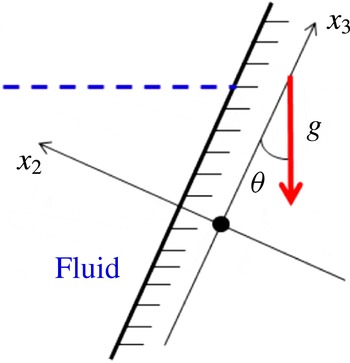
(figure 1) (Yih Reference Yih1966; Constantin Reference Constantin2001b
). When
 ${\it\theta}=0$
, (4.1) describes either a surface wave in a fluid half-space with a surface at
 $a_{2}=a_{2}^{(0)}$
(Lamb Reference Lamb1932, Chapter 9; Constantin Reference Constantin2001a
), if
 $-\infty <a_{3}<\infty$
, or a wave propagating along a rigid vertical boundary, if
 $-\infty <a_{3}\leqslant 0$
. The flow is two-dimensional; projection of the fluid velocity
 $\partial \boldsymbol{x}/\partial t$
on the
 $x_{2}$
coordinate axis is identically zero. The flow is rotational; its vorticity
 $kc\exp (ka_{2})/\text{sinh}\,ka_{2}$
is maximum at the surface
 $a_{2}=a_{2}^{(0)}$
and rapidly decreases with increasing
 $|a_{2}|$
(Lamb Reference Lamb1932). The wave field is periodic in time and in
 $x_{1}$
, and the wave period and wavelength are equal to
 $2{\rm\pi}/kc$
and
 $2{\rm\pi}/k$
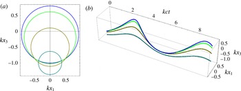
respectively. The kinematics of the flow is illustrated in figure 2. It has been rigorously established (Constantin Reference Constantin2001a
,Reference Constantin
b
; Henry Reference Henry2008) that, with the mapping (4.1), fluid parcels never collide and fill the entire domain under the surface
 $\boldsymbol{x}=\boldsymbol{x}(a_{1},\;a_{2}=a_{2}^{(0)},\;a_{3},\;t)$
. If the condition
 $a_{2}<0$
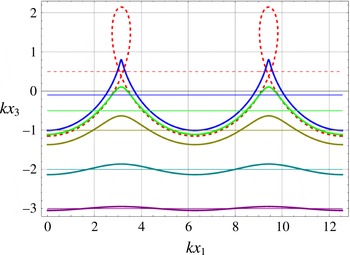
were not met, the mapping (4.1) of the Lagrangian coordinates into the coordinate space would not be one-to-one, and two fluid parcels would simultaneously occupy the same location, which is physically impossible (figure 3).
The geometry of the edge wave problem. The dashed line shows the free surface of the fluid in the absence of waves.

Trajectories of fluid parcels in a nonlinear surface wave. The trajectories are shown in non-dimensional variables for
 $ka_{1}=0$
,
 $ka_{3}=-0.1,-0.2,-0.5$
and
 $-1$
. In the
 $x_{1}x_{3}$
plane, fluid parcels rotate counterclockwise in waves propagating towards decreasing
 $x_{1}$
, with the radius of circular trajectories decreasing exponentially with
 $ka_{3}$
.

Surfaces of constant pressure and constant density in a nonlinear surface wave propagating along the
 $x_{1}$
axis (thick lines) and in the absence of waves (thin lines). The surfaces are
 $2{\rm\pi}$
-periodic functions of
 $k(x_{1}+ct)$
and are shown at time
 $t=0$
for
 $ka_{2}=0.5$
(dashed lines),
 $-0.1,-0.5,-1,-2$
and
 $-3$
. The wave motion is physically realizable only at
 $a_{2}\leqslant a_{2}^{(0)}<0$
.

To demonstrate that the flow (4.1) is dynamically feasible, we first note that the Jacobian
 $J\equiv \partial (x_{1},x_{2},x_{3})/\partial (a_{1},a_{2},a_{3})=1-\exp (2ka_{2})$
is independent of time. It ensures that (3.2) is met and the flow is incompressible. Upon substitution of the trajectories
 $\boldsymbol{x}(t)$
(4.1) into the Euler equation (3.1), the dispersion relation (4.2) ensures that time-dependent terms cancel out, and (3.1) becomes
 $$\begin{eqnarray}\frac{\partial p}{\partial a_{1}}=0,\quad \frac{\partial p}{\partial a_{2}}=-(1-\text{e}^{2ka_{2}}){\it\rho}g\cos {\it\theta},\quad \frac{\partial p}{\partial a_{3}}={\it\rho}g\sin {\it\theta}.\end{eqnarray}$$
The Euler equation (3.1) as well as (3.3) and (3.4) will be satisfied if
 $$\begin{eqnarray}p=gf(b),\quad {\it\rho}=-f^{\prime }(b),\quad b=a_{2}(1-\text{e}^{2ka_{2}})\cos {\it\theta}-a_{3}\sin {\it\theta},\end{eqnarray}$$
where
 $f(b)\geqslant 0$
is any steadily decreasing differentiable function. Here and below, a prime denotes the derivative of a function with respect to its argument. It should be noted that
 $p$
varies continuously in space, while continuity of
 ${\it\rho}$
is not required. According to (4.4), surfaces of constant pressure and constant density coincide. (In geophysical literature, waves possessing such a property are referred to as barotropic.) The curves that are formed by intersection of these surfaces with the plane
 $x_{2}=\text{const.}$
are trochoids, the limiting form of which at
 $a_{2}=0$
is a cycloid (Lamb Reference Lamb1932, Article 251). As
 $a_{2}\rightarrow -\infty$
, wave-induced acceleration of fluid parcels tends to zero, and the surfaces
 $b=\text{const.}$
of constant pressure approach their static limit, i.e. horizontal planes
 $x_{2}\sin {\it\theta}+x_{3}\cos {\it\theta}=\text{const.}$
(figure 3). When
 $0<{\it\theta}<{\rm\pi}/2$
, any surface
 $b=b_{0}$
, where
 $b_{0}=\text{const.}$
, can be chosen as the free surface (or, more generally, as a surface under constant external pressure, such as the ocean surface under atmospheric pressure), which limits the extent of the fluid from above. When
 ${\it\theta}=0$
, the maximum possible value of
 $b_{0}$
is
 $a_{2}^{(0)}[1-\exp (2ka_{2}^{(0)})]$
.
In the case of incompressible fluids, derivation of (4.4) completes the proof that the motion (4.1) is dynamically possible. For compressible fluids, the function
 $f$
is not arbitrary and should be determined from the equation of state. For instance, in an ideal gas with the ratio
 ${\it\gamma}$
of specific heats at constant pressure and constant volume,
 ${\it\gamma}p={\it\rho}C^{2}$
(Lamb Reference Lamb1932), where
 $C=[(\partial p/\partial {\it\rho})_{S}]^{1/2}$
is the sound speed. Then, from (4.4) we find that
 $$\begin{eqnarray}p(b)=p(b_{0})\exp \left(g\int _{b}^{b_{0}}{\it\gamma}(b_{1})C^{-2}(b_{1})\text{d}b_{1}\right),\quad {\it\rho}(b)={\it\gamma}(b)C^{-2}(b)p(b)\end{eqnarray}$$
for the incompressible wave motion in an ideal gas.
In isentropic fluids, where the entropy density
 $S=\text{const.}$
, as well as in fluids with the so-called barotropic equation of state, where the pressure
 $p=p({\it\rho})$
and is independent of
 $S$
, from (4.4) and the definition of the sound speed, we find that
 $gf^{\prime }=-C^{2}f^{\prime \prime }$
, which leads to the following expressions for pressure and density in the wave:
 $$\begin{eqnarray}\displaystyle p(b)=p(b_{0})+g{\it\rho}(b_{0})\int _{b}^{b_{0}}\text{d}b_{1}\exp \left(\int _{b_{1}}^{b_{0}}\frac{g\text{d}b_{2}}{C^{2}(b_{2})}\right),\quad {\it\rho}(b)={\it\rho}(b_{0})\exp \left(\int _{b}^{b_{0}}\frac{g\text{d}b_{2}}{C^{2}(b_{2})}\right)\!. & & \displaystyle \nonumber\\ \displaystyle & & \displaystyle\end{eqnarray}$$
The sound speed
 $C(b)$
is generally not known in advance. Our use of the sound speed in (4.5) and (4.6) parallels the treatment of the equation of state in the other known exact solution for nonlinear waves in compressible fluids, Riemann’s ‘simple wave’ (Riemann Reference Riemann1858; Landau & Lifshitz Reference Landau and Lifshitz2004, § 101). Despite
 $C(b)$
being unknown, (4.5) and (4.6) offer some insight into the variation of the pressure and density with
 $b$
, especially when relative variations of the sound speed are much smaller than relative variations of the pressure (as is the case in the ocean) or of the pressure and density (as is the case in the atmosphere).
It is instructive to compare (4.2) with the form that the Euler equation (3.1) takes in the case of stationary fluid. A description of the static equilibrium in a gravity field is formally obtained by replacing
 $\exp (ka_{2})$
with zero in (4.1) and (4.3). Then, solutions for the pressure and density are again given by (4.4), which in the static equilibrium becomes
 $$\begin{eqnarray}p=gf(B),\quad {\it\rho}=-f^{\prime }(B),\quad B=x_{2}\sin {\it\theta}+x_{3}\cos {\it\theta}.\end{eqnarray}$$
As expected, the surfaces of constant static pressure and density are planes orthogonal to
 $\boldsymbol{g}$
. The minimum value of the pressure is attained on the surface of the fluid and, as in the case of wave motion, equals the constant external pressure
 $P_{0}$
. Equation (4.7) shows that solution (4.4) to simultaneous equations (4.3) exists and, therefore, the wave motion (4.1) is possible in any compressible ideal fluid that can sustain a static equilibrium in the uniform gravity field, i.e. essentially any physically realizable fluid. Furthermore, if the wave (4.1) is generated from a static equilibrium by an action of external forces, the pressure and density fields in the wave are obtained from the hydrostatic profiles
 $p(B)$
and
 ${\it\rho}(B)$
by replacing
 $B(x_{2},x_{3})$
(4.7) with
 $b(x_{1},x_{2},x_{3},t)$
(4.4).
Consider, for instance, a polytropic ideal gas, where (Landau & Lifshitz Reference Landau and Lifshitz2004, § 83)
 $$\begin{eqnarray}p{\it\rho}^{-n}=\text{const.}\end{eqnarray}$$
and the ratio of the specific heats
 ${\it\gamma}$
is constant. The constant
 $n$
is referred to as the polytropic index. The polytropic gas model is often used in gas dynamics and astrophysics (Christensen-Dalsgaard et al.
Reference Christensen-Dalsgaard, Duvall, Gough, Harvey and Rhodes1985; Landau & Lifshitz Reference Landau and Lifshitz2004, Chapters 9, 10 and 14) as well as in theoretical investigations of linear acoustic-gravity waves in a stratified atmosphere (Lamb Reference Lamb1932, Articles 310, 312, 315; Pekeris Reference Pekeris1948; Price Reference Price1992). In hydrostatic equilibrium, the temperature and sound speed are linear functions of
 $B$
in polytropic gases (Price Reference Price1992). From the known hydrostatic profiles of pressure and density in polytropic gases (or immediately from (4.7) and (4.8)), we find the pressure and density distributions in the nonlinear incompressible wave motion (4.1):
 $$\begin{eqnarray}p(b)=\left[1+\frac{n-1}{n}\frac{{\it\rho}(b_{0})}{p(b_{0})}(b-b_{0})\right]^{\;n/(n-1)}p(b_{0}),\quad {\it\rho}(b)=\left[\frac{p(b)}{p(b_{0})}\right]^{1/n}{\it\rho}(b_{0}).\end{eqnarray}$$
Here, the surface values of the pressure,
 $p(b_{0})=P_{0}$
, and density,
 ${\it\rho}(b_{0})$
, are assumed to be known. In particular, in the case of an isothermal atmosphere, where
 $n=1$
and the sound speed
 $C$
is constant, (4.9) gives
 $p(b)=\exp [{\it\gamma}g(b_{0}-b)/C^{2}]p(b_{0})$
, in agreement with (4.5). In the case of an adiabatic (i.e. isentropic) atmosphere, where
 $n={\it\gamma}$
(Landau & Lifshitz Reference Landau and Lifshitz2004, § 83), (4.9) gives
 $p(b)=[1+({\it\gamma}-1)(b_{0}-b)g/C^{2}(b_{0})]^{{\it\gamma}/({\it\gamma}-1)}$
 $p(b_{0})$
, in agreement with (4.6).
4.2. Waves in a background flow
We now extend the exact solutions given by (4.1), (4.5) and (4.6) to progressive surface waves in moving fluids. This is motivated by the recent finding for linear waves (Godin Reference Godin2014) that incompressible wave motion remains possible in the presence of certain inhomogeneous background flows.
Let
 $\boldsymbol{g}=(0,0,-g)$
and consider a fluid motion, which is described in the Lagrangian representation by the equations
 $$\begin{eqnarray}\left.\begin{array}{@{}c@{}}x_{1}=a_{1}+vt+\text{e}^{ka_{2}}{\displaystyle \frac{\sin {\it\varphi}}{k}},\quad x_{2}=u(a_{1},a_{2})t-a_{3},\\ x_{3}=a_{2}-\text{e}^{ka_{2}}{\displaystyle \frac{\cos {\it\varphi}}{k}},\quad {\it\varphi}=k(a_{1}+ct+vt),\end{array}\right\}\end{eqnarray}$$
where
 $-\infty <a_{1,\,3}<\infty$
and
 $-\infty <a_{2}\leqslant a_{2}^{(0)}<0$
. Unlike (4.1), the flow (4.10) is three-dimensional. Equation (4.10) represents a wave propagating horizontally in a fluid with a steady horizontal current, with components
 $v$
and
 $u$
respectively along and across the wave propagation direction. When
 $u=v=0$
, (4.10) reduces to (4.1).
For the flow (4.10), the Jacobian
 $J=1-\exp (2ka_{2})$
, as is the case for the flow (4.1). The Jacobian is positive, which ensures one-to-one mapping between the Lagrangian and Cartesian coordinates. Substitution of the trajectories
 $\boldsymbol{x}(t)$
(4.10) into the Euler equation (3.1) gives
 $$\begin{eqnarray}\displaystyle \left.\begin{array}{@{}c@{}}\displaystyle \frac{1}{{\it\rho}}\frac{\partial p}{\partial a_{1}}=\text{e}^{ka_{2}}[k(c+v)^{2}-g]\sin {\it\varphi},\quad \frac{\partial p}{\partial a_{3}}=0,\\ \displaystyle \frac{1}{{\it\rho}}\frac{\partial p}{\partial a_{2}}=\text{e}^{ka_{2}}[k(c+v)^{2}-g]\cos {\it\varphi}+\text{e}^{2ka_{2}}k(c+v)^{2}-g.\end{array}\right\} & & \displaystyle\end{eqnarray}$$
It follows from (3.3) and (3.4) that the left-hand sides of (4.11) are time-independent, leading to the dispersion equation
 $k(c+v)^{2}=g$
of the wave. Then, (4.11) is satisfied, when
 $p$
and
 ${\it\rho}$
are given by (4.4) (with
 ${\it\theta}=0$
). Thus, the wave field (4.4), (4.10) provides an exact solution of the Euler and continuity equations (3.1) and (3.3). Equations (4.5) and (4.6) remain unchanged and ensure that the equation of state is met in compressible fluids. As in the case
 $u=v=0$
, surfaces of constant pressure and constant density (figure 3) coincide and move with the speed
 $c$
towards negative
 $x_{1}$
without changing their shape. It should be noted that, as in the case of linear waves (Godin Reference Godin2014), the transverse current
 $u(a_{1},a_{2})$
does not affect either the dispersion relation or the pressure and density fields.
According to the dispersion relation, the nonlinear wave has the same speed
 $c$
and wavelength
 $2{\rm\pi}/k$
for two different values of the current component
 $v:\;v_{1,2}=-c\pm (g/k)^{1/2}$
. So far, it has been assumed that
 $v$
is constant. Now we show that the exact solution obtained above also represents incompressible wave motion in a more general problem, where
 $v$
is a discontinuous function of
 $a_{2}$
, which alternates between values
 $v_{1}$
and
 $v_{2}$
. Let
 $v$
be discontinuous at
 $a_{2}=A$
. For trajectories of fluid parcels above and below this interface, from (4.10) we have
 $$\begin{eqnarray}\displaystyle x_{1}^{(m)}=\frac{{\it\varphi}_{m}}{k}-ct+\text{e}^{ka_{2}}\frac{\sin {\it\varphi}_{m}}{k},\quad x_{3}^{(m)}=a_{2}-\text{e}^{ka_{2}}\frac{\cos {\it\varphi}_{m}}{k},\quad {\it\varphi}_{m}=k\left[a_{1}^{(m)}-(-1)^{m}t\sqrt{\frac{g}{k}}\,\right], & & \displaystyle \nonumber\\ \displaystyle & & \displaystyle\end{eqnarray}$$
where
 $m=1$
and
 $m=2$
correspond to
 $v_{1}$
and
 $v_{2}$
respectively. The transverse current
 $u$
does not affect the geometry of the interface, which is invariant with respect to translations along the
 $x_{2}$
coordinate. Comparison of (4.3) and (4.11) shows that the background flow does not affect the pressure distribution as long as the dispersion equation
 $k(c+v)^{2}=g$
holds.
We have already demonstrated that the fluid motion above and below the interface satisfies continuity, state and Euler equations, so it remains to check whether boundary conditions are met on the interface. Since
 $a_{2}=\text{const.}$
are surfaces of constant pressure, fulfilment of the dynamic boundary condition of pressure continuity across the interface is ensured by (4.4). The kinematic boundary condition can be formulated as the requirement that the surfaces
 $a_{2}=A$
defined by (4.12) with
 $m=1$
and
 $m=2$
coincide at all times. According to (4.12),
 ${\it\varphi}_{m}$
is a steadily increasing function of
 $x_{1}^{(m)}$
, when
 $t$
and
 $a_{2}$
are fixed. Hence, from
 $x_{1}^{(1)}=x_{1}^{(2)}$
it follows that
 ${\it\varphi}_{1}={\it\varphi}_{2}$
. (This occurs when
 $a_{1}^{(2)}-a_{1}^{(1)}=2(g/k)^{1/2}t$
, see (4.12c
).) Then, according to (4.12b
),
 $x_{3}^{(1)}=x_{3}^{(2)}$
, which verifies the kinematic boundary condition. A different argument leading to the same conclusion was advanced by Mollo-Christensen (Reference Mollo-Christensen1982) in the context of Gerstner waves in incompressible fluids.
The physics of the solution (4.12) with a discontinuous mean flow is actually rather simple. Consider two fluids at rest, with a Gerstner-type wave propagating to the left in one fluid and to the right in the other. When the specific mean flows
 $v_{1}$
and
 $v_{2}$
are added, the propagation velocities of the two wave solutions become identical, and the solutions can be joined across the interface of the two fluids.
It should be noted that there exists an exact solution (4.4), (4.10) for arbitrary
 $v_{1}$
and
 $v_{2}$
. In such a wave,
 $c=-(v_{1}+v_{2})/2$
and
 $k=4g(v_{1}-v_{2})^{-2}$
. The wave is progressive, when
 $v_{1}+v_{2}\neq 0$
, and standing, when
 $v_{1}+v_{2}=0$
.
Quite similarly, one can show that (4.10) (with
 $u\equiv 0$
) and (4.4) describe an edge wave in a compressible fluid with a sloping rigid boundary
 $x_{2}=0$
and a steady current
 $v$
along the direction of the wave propagation. In the geometry of figure 1, the dispersion equation of the edge wave is given by
 $k(c+v)^{2}=g\cos {\it\theta}$
.
5. Discussion
Lamb (Reference Lamb1932) emphasized that, as it has non-zero vorticity, the Gerstner wave cannot be generated from rest by conservative forces in an ideal fluid. He noted that ‘The circumstance …that the motion in these waves is not irrotational detracts somewhat from the physical interest of the results’ and that a rather specific initial horizontal motion would be needed for the Gerstner surface wave to be generated by a distribution of pressure applied to the surface (Lamb Reference Lamb1932, Article 251). Lamb’s argument led to Gerstner waves often been treated as just a mathematical oddity.
Constantin (Reference Constantin2001b ) argued, however, that Gerstner edge waves correctly reproduce observations of key properties of coastally trapped waves in the ocean. Weber (Reference Weber2012) pointed out that Lamb’s argument is ‘less weighty’ when applied to edge waves since vorticity is always present in strongly nonlinear nearshore processes. In thorough laboratory experiments, Monismith et al. (Reference Monismith, Cowen, Nepf, Magnaudet and Thais2007) found that Gerstner waves, rather than irrotational Stokes waves, provide ‘a simple and accurate description’ of their observations of mechanically generated deep-water surface waves.
It should be noted that Lamb’s reasoning does not apply to wave generation in the presence of generic background stratified flows and, in particular, to the Gerstner waves in background flows we have considered in § 4.2. One can imagine Gerstner-like waves being generated in the ocean, together with other waves, by winds over a shear current, and the Gerstner-like waves subsequently separating from the other wave components (due to differences in speed or direction of propagation) and eventually travelling away from the shear current. When Gerstner waves are generated simultaneously with other waves rather than in isolation, the specific vorticity profile of the initial flow, which was derived by Lamb (Reference Lamb1932), is no longer required. Another scenario for Gerstner wave emergence was suggested by Pollard (Reference Pollard1970). He argued that, under the action of the Coriolis force, irrotationally generated Stokes waves change to Gerstner-like waves within a quarter of an inertial period (Pollard Reference Pollard1970).
The above discussion refers to waves in incompressible fluids. The situation is rather different for waves in compressible fluids as these waves are, as a rule, rotational in stably stratified fluids. Therefore, the non-zero vorticity of Gerstner acoustic-gravity waves we derived in § 4 cannot be viewed as a shortcoming of these exact solutions. Even linear acoustic-gravity waves are generally rotational (Pekeris Reference Pekeris1948). This is especially clear for acoustic waves in stratified fluids, where linearization of the Euler equation (2.1) gives
 $\partial \boldsymbol{v}/\partial t=-\boldsymbol{{\rm\nabla}}p/{\it\rho}_{0}$
in the Eulerian representation. Here,
 ${\it\rho}_{0}$
is the fluid density undisturbed by the waves. Let the density be a continuously differentiable function of the vertical Cartesian coordinate
 $x_{3}$
. Application of the differential operator curl to the linearized Euler equation makes it obvious that the velocity potential does not exist except for one-dimensional vertical wave motion. Now consider continuous linear acoustic-gravity waves with the harmonic dependence
 $\exp (\text{i}\boldsymbol{k}\boldsymbol{\cdot }\boldsymbol{x}-\text{i}{\it\omega}t)$
, with
 $\boldsymbol{k}=(k_{1},k_{2},0)$
, on horizontal coordinates and time in a vertically stratified fluid;
 $\boldsymbol{g}=(0,0,-g)$
. Linearized equations of motion can be written as (e.g. Gill Reference Gill1982)
 $$\begin{eqnarray}\displaystyle & \displaystyle \frac{\partial p}{\partial x_{3}}+\frac{g}{C_{0}^{2}}p=\frac{\text{i}{\it\rho}_{0}}{{\it\omega}}({\it\omega}^{2}-N^{2})v_{3}, & \displaystyle\end{eqnarray}$$
 $$\begin{eqnarray}\displaystyle & \displaystyle \frac{\partial v_{3}}{\partial x_{3}}-\frac{g}{C_{0}^{2}}v_{3}=\left(\frac{1}{C_{0}^{2}}-\frac{k^{2}}{{\it\omega}^{2}}\right)\frac{\text{i}{\it\omega}p}{{\it\rho}_{0}}, & \displaystyle\end{eqnarray}$$
 $v_{j}=k_{j}p/{\it\omega}{\it\rho}_{0},~j=1,2$
. Here,
 $c_{0}$
is the sound speed undisturbed by waves and
 $N$
is the buoyancy frequency,
 $N^{2}=-g{\it\rho}_{0}^{-1}\text{d}{\it\rho}_{0}/\text{d}x_{3}-g^{2}C_{0}^{-2}$
. In stably and neutrally stratified fluids
 $N^{2}\geqslant 0$
(Gill Reference Gill1982). It follows from (5.1) and (5.2) that
 $$\begin{eqnarray}{\it\rho}_{0}g{\it\omega}\boldsymbol{k}\times \text{curl}~\boldsymbol{v}=k^{2}N^{2}\tilde{p}\boldsymbol{e}_{3},\end{eqnarray}$$
where
 $\tilde{p}=p-\text{i}{\it\omega}^{-1}{\it\rho}_{0}gv_{3}$
is the wave-induced perturbation of pressure in moving fluid parcels, i.e. the Lagrangian pressure perturbation. Equation (5.3) shows that, except for purely vertical flows (
 $k=0$
), wave motion in a stratified compressible inviscid fluid has non-zero vorticity unless either
 $\tilde{p}\equiv 0$
(Godin Reference Godin2012) or
 $N\equiv 0$
.
It is natural to wonder whether acoustic-gravity waves with properties that which are similar to those described in § 4 have been observed experimentally. Any systematic analysis of experimental data is, however, beyond the scope of this paper. Here, we discuss briefly just one example: ‘a fast external atmospheric acoustic-gravity wave’ described by Hecht et al. (Reference Hecht, Walterscheid, Hickey, Rudy and Liu2002). The wave observations were made with a near-infrared airglow imaging system located at the Starfire Optical Range in New Mexico, USA. A wind and temperature lidar was operating simultaneously at the range providing wind and temperature data up to nearly 110 km altitude (Hecht et al.
Reference Hecht, Walterscheid, Hickey, Rudy and Liu2002). The observed wave period, phase velocity and wavelength were
 $2{\rm\pi}/kc=215\pm 10~\text{s}$
,
 $c=160\pm 10~\text{m}~\text{s}^{-1}$
and
 $2{\rm\pi}/k=35\pm 2~\text{km}$
. The wave frequency was of the order of but larger than the buoyancy frequency. Because of the relatively short period of the wave and its large phase speed, air compressibility was supposed to play a significant role (Hecht et al.
Reference Hecht, Walterscheid, Hickey, Rudy and Liu2002). The observations were remarkable because of the relatively large magnitude, phase velocity and frequency of the wave compared with other airglow-based observations. With frequencies above the buoyancy frequency and the phase speed smaller than the sound speed, the wave was expected to be evanescent with height and propagate horizontally as opposed to waves propagating in the vertical direction. As was pointed out by Hecht et al. (Reference Hecht, Walterscheid, Hickey, Rudy and Liu2002), the presence of the ground surface had a negligible effect on the wave because of a rapid exponential increase of its amplitude with height. Numerical simulations (Hecht et al.
Reference Hecht, Walterscheid, Hickey, Rudy and Liu2002) showed that the observed wave parameters were not affected by artificially truncating the atmosphere and placing an upper boundary at 350 km altitude.
The observed wave parameters satisfy the dispersion equation
 $k(c+v)^{2}=g$
, which was derived in § 4.2, provided that
 $v=-71\pm 12~\text{m}~\text{s}^{-1}$
. This value is consistent with the sign and magnitude of the wind velocity in the direction of wave propagation during the experiment around the 100 km height (see figure 3 in Hecht et al.
Reference Hecht, Walterscheid, Hickey, Rudy and Liu2002), where the wave is believed to be generated by a Leonids meteor. Thus, it appears that the finite-amplitude incompressible wave motion provides a reasonable initial approximation to and interpretation of the atmospheric wave identified by Hecht et al. (Reference Hecht, Walterscheid, Hickey, Rudy and Liu2002) in their airglow measurements.
Exact wave solutions, and especially solutions for nonlinear waves (Gerstner Reference Gerstner1809; Riemann Reference Riemann1858; Yih Reference Yih1966; Pollard Reference Pollard1970; Kinnersley Reference Kinnersley1976; Chernyak, Karelsky & Petrosyan Reference Chernyak, Karelsky and Petrosyan2013), are exceedingly rare. These solutions refer to highly idealized models and invariably require strong assumptions, such as the assumption of an infinite plane rigid boundary for Gerstner edge waves, which can be met only approximately in the physical world. Even if Gerstner-like waves are observed only infrequently, Gerstner waves and, arguably, their extension to compressible fluids are of significant educational and scientific value because of their simplicity and the opportunities they provide for theoretical studies (Johnson Reference Johnson2005) and verification of numerical models.
6. Conclusion
We have demonstrated that compressible fluids in a uniform gravity field support finite-amplitude incompressible wave motion, in which pressure and density remain constant in each moving fluid parcel. An exact explicit solution is obtained which describes surface and edge waves of this kind. To the best of our knowledge, this is the first exact analytic solution of full hydrodynamic equations for nonlinear progressive waves in stratified compressible fluids in a gravity field. The solution applies to rather general inhomogeneous fluids and allows for discontinuities in sound speed, density and flow velocity; this is particularly important for applications to acoustic-gravity waves in a coupled ocean–atmosphere system. The nonlinear wave reduces to an appropriate linear solution (Godin Reference Godin2012, Reference Godin2014) in the limit of a vanishing amplitude. In another limit of an incompressible fluid, the new solution provides an extension of Gerstner waves (Dubreil-Jacotin Reference Dubreil-Jacotin1932; Lamb Reference Lamb1932, Chapter 9; Yih Reference Yih1966; Mollo-Christensen Reference Mollo-Christensen1982; Constantin Reference Constantin2001a ,Reference Constantin b ; Henry Reference Henry2008; Stuhlmeier Reference Stuhlmeier2011) to nonlinear waves in the presence of stationary currents (winds).
The exact solution for finite-amplitude acoustic-gravity waves enhances our physical understanding of wave types supported by the ocean and atmosphere, can be used to evaluate various approximate methods in the theory of nonlinear waves and provides a benchmark for numerical models of compressible fluid dynamics.
Acknowledgements
Stimulating discussions with M. Charnotskii and I. M. Fuks are gratefully acknowledged. I am indebted to O. Buhler and two anonymous reviewers for valuable suggestions and helpful criticism of an early version of the paper. This research has been supported in part by the Office of Naval Research, grant N00014-13-1-0348.