





1. Introduction
Shallow granular free-surface flows are one of the most common particle transport mechanisms in both our natural environment and industry. Hazardous geophysical mass flows such as snow avalanches (Savage & Hutter Reference Savage and Hutter1989; Ancey Reference Ancey2012), debris flows (Iverson Reference Iverson1997), rockfalls, pyroclastic flows (Branney & Kokelaar Reference Branney and Kokelaar1992) and lahars (Vallance Reference Vallance2000) all fall into this category, while in industry examples include chute flows (Pouliquen Reference Pouliquen1999a ) as well as thin fluid-like avalanches that develop in the free-surface layers of heaps (Williams Reference Williams1968), silos (Schulze Reference Schulze2008) and rotating tumblers (Gray & Hutter Reference Gray and Hutter1997; Hill et al. Reference Hill, Kharkar, Gilchrist, McCarthy and Ottino1999). It is precisely these granular avalanches that are particularly efficient at segregating particles by size (Middleton Reference Middleton and Lajoie1970; Savage & Lun Reference Savage and Lun1988) and density differences between the particles (Drahun & Bridgwater Reference Drahun and Bridgwater1983). Despite many years of research, both particle size and density segregation continue to present considerable practical problems in many industrial processes (Johanson Reference Johanson1978; Gray Reference Gray2010). Sometimes the segregation is useful, such as in the mining industry (Wills Reference Wills1979), but mostly it is undesired and it can degrade the quality of products, leading to increased costs and considerable wastage.
An ability to predict segregation is the first step in understanding the phenomenon and ultimately being able to design equipment to either enhance or mitigate its effect. Early continuum models for particle-size segregation were first formulated by Bridgwater, Foo & Stephens (Reference Bridgwater, Foo and Stephens1985). Their very simple one-dimensional time-dependent model consisted of an advection diffusion equation for the concentration of one of the species, with a flux function that shut off when the concentration reached zero or unity. This essential structure is still present in current bidisperse segregation models. Savage & Lun (Reference Savage and Lun1988) used an information entropy approach to model particle-size segregation. They argued that the avalanche acted as a ‘random fluctuating sieve’ in which small particles were statistically more likely to fall down into gaps than large grains, as particles were sheared over one another. This led to differential percolation rates of the large and small particles; this was opposed by a mechanism called ‘squeeze expulsion’, which gave an equal probability for all particles to be levered upwards. When these two processes were combined, there was a net flux of small particles to the base of the flow and a net flux of large particles towards the surface. It is not immediately apparent, but Savage & Lun’s (Reference Savage and Lun1988) theory is, in fact, closely related to that of Bridgwater et al. (Reference Bridgwater, Foo and Stephens1985). This is because the flux functions appear to be much more complicated and the model was formulated in terms of number densities rather than concentrations. For a prescribed downstream velocity field Savage & Lun’s (Reference Savage and Lun1988) theory was able to compute the steady-state size distribution in a chute flow which was in good agreement with experiments that took relatively coarse resolution samples by using a movable hopper, splitter plates and a binning procedure. Dolgunin & Ukolov (Reference Dolgunin and Ukolov1995) postulated a model that was based on the simple observation that the segregation must shut off when the concentration reaches zero or unity. This was very much in the spirit of Bridgwater et al.’s (Reference Bridgwater, Foo and Stephens1985) approach, but it was two-dimensional, time-dependent and included the effects of particle diffusion.
Over recent years there has been a lot of work on developing models for particle-size segregation from mixture theory. A review of this approach together with a detailed discussion of how it relates to earlier work is provided by Gray, Gajjar & Kokelaar (Reference Gray, Gajjar and Kokelaar2015). Mixture theory provides a useful framework, with clear definitions of intrinsic and mixture quantities as well as individual mass and momentum conservation laws for each species of particle. Gray & Thornton (Reference Gray and Thornton2005) formulated a theory for bidisperse segregation in which the interstitial pore space was implicitly incorporated into the bulk density of the particles, while Thornton, Gray & Hogg (Reference Thornton, Gray and Hogg2006) explicitly included the air by using a three-phase mixture theory. Gray & Chugunov (Reference Gray and Chugunov2006) showed how to include diffusive remixing of the particles into the theory, and used the Cole–Hopf transformation (Hopf Reference Hopf1950; Cole Reference Cole1951) to construct exact time and spatially dependent solutions with diffusion. All of these theories are closely related to those of Bridgwater et al. (Reference Bridgwater, Foo and Stephens1985), Savage & Lun (Reference Savage and Lun1988) and Dolgunin & Ukolov (Reference Dolgunin and Ukolov1995), but provide a much more detailed derivation that can easily be extended to other situations. Although the theories are relatively simple, they are able to accurately model the concentration distribution in chute flow experiments. Wiederseiner et al. (Reference Wiederseiner, Andreini, Epely-Chauvin, Moser, Monnereau, Gray and Ancey2011) averaged 2000 high-speed camera images taken through a transparent sidewall at 10 downstream locations along a chute and used a calibration curve to build up a complete picture of the spatial evolution of the particle-size distribution. They showed that the theory was able to accurately capture the complete spatial evolution from a normally graded inflow (with all the small particles on top of the large grains) to a reverse-graded steady-state distribution sufficiently far downstream (in which large particles were concentrated in the surface layers). Typical Péclet numbers for segregation were found to be in the range 11–19, with complete segregation occurring 70 cm downstream for a flow of depth 24 mm. The theory has also been able to accurately match time-dependent segregation data derived from discrete particle method (DPM) simulations performed on a periodic box (Thornton et al. Reference Thornton, Weinhart, Luding and Bokhove2012; Staron & Phillips Reference Staron and Phillips2014). While there is considerable scope for developing more experimental and DPM data sets to help in calibrating the parameters in the models, the work of Wiederseiner et al. (Reference Wiederseiner, Andreini, Epely-Chauvin, Moser, Monnereau, Gray and Ancey2011), Thornton et al. (Reference Thornton, Weinhart, Luding and Bokhove2012) and Staron & Phillips (Reference Staron and Phillips2014) provides very strong evidence that the segregation models have the correct underlying mathematical structure.
Simple insights into the nature of segregation are provided by the non-diffuse theory, which allows exact two-dimensional time-dependent solutions (Gray, Shearer & Thornton Reference Gray, Shearer and Thornton2006; Shearer, Gray & Thornton Reference Shearer, Gray and Thornton2008) to be constructed, as well as steadily travelling breaking waves (Thornton & Gray Reference Thornton and Gray2008; Gray & Ancey Reference Gray and Ancey2009; Johnson et al. Reference Johnson, Kokelaar, Iverson, Logan, LaHusen and Gray2012). These develop as small particles are sheared over large grains and play an important role near flow fronts. The theory has also been depth averaged (Gray & Kokelaar Reference Gray and Kokelaar2010a ,Reference Gray and Kokelaar b ) to provide a simplified description of large-particle transport, which facilitates easy coupling to depth-averaged avalanche models (e.g. Gray & Edwards Reference Gray and Edwards2014), which can be used to study segregation–mobility feedback effects that lead to flow fingering (Pouliquen, Delour & Savage Reference Pouliquen, Delour and Savage1997; Pouliquen & Vallance Reference Pouliquen and Vallance1999; Woodhouse et al. Reference Woodhouse, Thornton, Johnson, Kokelaar and Gray2012).
Fan & Hill (Reference Fan and Hill2011) have extended the theory to shear-induced, rather than gravity-driven, segregation and Tripathi & Khakhar (Reference Tripathi and Khakhar2013) have derived a theory for pure density segregation that has a similar structure to the size-segregation models. In addition, Gray & Ancey (Reference Gray and Ancey2011) and Marks, Rognon & Einav (Reference Marks, Rognon and Einav2012) have generalized the theory to polydisperse systems, with both discrete grain-size classes and continuous distributions. The size-segregation theory of Marks et al. (Reference Marks, Rognon and Einav2012) is particularly interesting, because it includes the effects of both particle size and particle density, although the combined effect was not explored in the paper. Tunuguntla, Bokhove & Thornton (Reference Tunuguntla, Bokhove and Thornton2014) have used this approach to derive a conservation law for bidisperse segregation which explicitly includes the effects of density differences between the particles. This is a distinctly non-trivial extension of the theory, because as the particles segregate the local density changes in response to the changing concentration of each species. As a result, the bulk velocity
 $\boldsymbol{u}$
is intimately linked to the evolving bulk density
 ${\it\rho}$
, i.e. the bulk flow is no longer incompressible, but is compressible. The bulk velocity field can therefore no longer be simply prescribed, but one component must be solved for at the same time as the concentration. This aspect was not picked up on by Tunuguntla et al. (Reference Tunuguntla, Bokhove and Thornton2014), who solved their model using a prescribed incompressible velocity field. As a result, mass was not properly conserved. This paper derives an alternative theory for particle size and density segregation that automatically accounts for bulk compressibility of the flow.
2. Derivation of the particle-size and -density segregation equations
2.1. Mixture framework
Consider a binary mixture composed of particles of differing size and density. The two species of particles will be denoted as phases
 $A$
and
 $B$
and their local volume fractions per unit mixture volume are defined as
 $$\begin{eqnarray}{\it\phi}^{a}\in [0,1]\quad \text{and}\quad {\it\phi}^{b}\in [0,1]\end{eqnarray}$$
respectively. When the volume fraction equals zero there is a complete absence of that phase, while a value of unity indicates 100 % concentration. For simplicity, phases
 $A$
and
 $B$
are assumed to occupy all of the available space, so that the local volume fractions sum to unity,
 $$\begin{eqnarray}{\it\phi}^{a}+{\it\phi}^{b}=1.\end{eqnarray}$$
This implicitly assumes that the solids volume fraction is constant and uniform throughout the flow and that it can be incorporated into the intrinsic density of
 $A$
and
 $B$
(see, e.g., Thornton et al.
Reference Thornton, Gray and Hogg2006). It should be noted that it is well known that particles of differing sizes may pack more closely together in static configurations (see, e.g., Herrmann, Mantica & Bessis Reference Herrmann, Mantica and Bessis1990). However, when the particles are sheared, DPM simulations suggest that mixed regions have only a very slightly higher solids volume fraction than the pure phases (Thornton et al.
Reference Thornton, Weinhart, Luding and Bokhove2012), so the assumption of constant uniform solids volume fraction is a reasonable first approximation.
Mixture theory is formulated in terms of partial variables, defined per unit mixture volume, which are linked to intrinsic variables, defined per unit volume of the pure phase (see, e.g., Truesdell Reference Truesdell1984; Morland Reference Morland1992). The partial density
 ${\it\rho}^{{\it\nu}}$
and intrinsic density
 ${\it\rho}^{{\it\nu}\ast }$
of constituent
 ${\it\nu}$
are necessarily linked by a linear volume fraction scaling, while the partial and intrinsic velocities,
 $\boldsymbol{u}^{{\it\nu}}$
and
 $\boldsymbol{u}^{{\it\nu}\ast }$
, are the same,
 $$\begin{eqnarray}{\it\rho}^{{\it\nu}}={\it\phi}^{{\it\nu}}{\it\rho}^{{\it\nu}\ast },\quad \boldsymbol{u}^{{\it\nu}}=\boldsymbol{u}^{{\it\nu}\ast },\quad {\it\nu}=a,b.\end{eqnarray}$$
Each of the phases satisfies mass and momentum conservation laws,
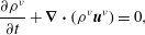 $$\begin{eqnarray}\displaystyle & \displaystyle \frac{\partial {\it\rho}^{{\it\nu}}}{\partial t}+\boldsymbol{{\rm\nabla}}\boldsymbol{\cdot }({\it\rho}^{{\it\nu}}\boldsymbol{u}^{{\it\nu}})=0, & \displaystyle\end{eqnarray}$$
 $$\begin{eqnarray}\displaystyle & \displaystyle \frac{\partial }{\partial t}({\it\rho}^{{\it\nu}}\boldsymbol{u}^{{\it\nu}})+\boldsymbol{{\rm\nabla}}\boldsymbol{\cdot }({\it\rho}^{{\it\nu}}\boldsymbol{u}^{{\it\nu}}\otimes \boldsymbol{u}^{{\it\nu}})=-\boldsymbol{{\rm\nabla}}p^{{\it\nu}}+{\it\rho}^{{\it\nu}}\boldsymbol{g}+{\bf\beta}^{{\it\nu}}, & \displaystyle\end{eqnarray}$$
 $\otimes$
is the dyadic product,
 $\boldsymbol{g}$
is the gravitational acceleration vector and
 $p^{{\it\nu}}$
is the partial pressure of constituent
 ${\it\nu}$
. It should be noted that deviatoric stresses have been neglected in (2.5) for simplicity. The interaction force
 ${\bf\beta}^{{\it\nu}}$
is the force exerted on phase
 ${\it\nu}$
by the other constituent and sums to zero over the two phases,
 $$\begin{eqnarray}{\bf\beta}^{a}+{\bf\beta}^{b}=\mathbf{0}.\end{eqnarray}$$
The bulk density
 ${\it\rho}$
, the barycentric velocity
 $\boldsymbol{u}$
and the bulk pressure
 $p$
are defined as
 $$\begin{eqnarray}{\it\rho}={\it\rho}^{a}+{\it\rho}^{b},\quad {\it\rho}\boldsymbol{u}={\it\rho}^{a}\boldsymbol{u}^{a}+{\it\rho}^{b}\boldsymbol{u}^{b},\quad p=p^{a}+p^{b}\end{eqnarray}$$
respectively. Summing the constituent mass balances over phases
 $A$
and
 $B$
yields an equation for the evolution of the bulk density,
 $$\begin{eqnarray}\frac{\partial {\it\rho}}{\partial t}+\boldsymbol{{\rm\nabla}}\boldsymbol{\cdot }({\it\rho}\boldsymbol{u})=0.\end{eqnarray}$$
When the intrinsic densities,
 ${\it\rho}^{a\ast }$
and
 ${\it\rho}^{b\ast }$
, are equal, (2.2), (2.3) and (2.7) imply that the bulk density
 ${\it\rho}={\it\rho}^{a\ast }={\it\rho}^{b\ast }$
, and the bulk mass balance (2.8) then implies that the bulk velocity field
 $\boldsymbol{u}$
is incompressible. When there is a density difference between the particles,
 ${\it\rho}^{a\ast }\neq {\it\rho}^{b\ast }$
, the bulk density
 ${\it\rho}$
is no longer constant and the bulk velocity field
 $\boldsymbol{u}$
is compressible. This a major departure from the assumptions of constant density and incompressibility, which are typically made in avalanche models (see, e.g., Grigorian, Eglit & Iakimov Reference Grigorian, Eglit and Iakimov1967; Savage & Hutter Reference Savage and Hutter1989; Iverson Reference Iverson1997; Gray, Wieland & Hutter Reference Gray, Wieland and Hutter1999; Pouliquen Reference Pouliquen1999a
,Reference Pouliquen
b
; Iverson & Denlinger Reference Iverson and Denlinger2001; Gray, Tai & Noelle Reference Gray, Tai and Noelle2003; Gray & Edwards Reference Gray and Edwards2014). It should be noted that mixture theory does not formally yield an equation for the bulk velocity field, by summing the constituent momentum balances, because the momentum transport terms cannot be rewritten just in terms of
 $\boldsymbol{u}$
. Instead, the constituent momentum balances must be solved for individually.
2.2. Mass fluxes and pressure perturbations
The grains are assumed to segregate as they avalanche down a slope inclined at an angle
 ${\it\zeta}$
to the horizontal, as shown in figure 1. A coordinate system
 $Oxyz$
is defined with the
 $x$
-axis pointing down the slope, the
 $y$
-axis pointing across it and the
 $z$
-axis being the upward-pointing normal. The components of the barycentric velocity
 $\boldsymbol{u}$
and constituent velocity
 $\boldsymbol{u}^{{\it\nu}}$
are defined as
 $(u,v,w)$
and
 $(u^{{\it\nu}},v^{{\it\nu}},w^{{\it\nu}})$
respectively. The avalanche is assumed to be shallow, so that the segregation velocity in the streamwise direction is negligible compared with the bulk velocity. Hence, the down- and cross-slope constituent velocity components are assumed to be equal to those of the bulk velocity in each of these directions,
 $$\begin{eqnarray}u^{{\it\nu}}=u,\quad v^{{\it\nu}}=v,\end{eqnarray}$$
which is consistent with measurements made in segregation experiments by Wiederseiner et al. (Reference Wiederseiner, Andreini, Epely-Chauvin, Moser, Monnereau, Gray and Ancey2011). In the normal direction phases
 $A$
and
 $B$
move relative to the bulk. The shallowness of the flow also implies that the normal acceleration terms are sufficiently small that they can be neglected. It follows that the sum of the normal momentum balances over phases
 $A$
and
 $B$
implies that the bulk pressure is lithostatic,
 $$\begin{eqnarray}\frac{\partial p}{\partial z}=-{\it\rho}g\cos {\it\zeta},\end{eqnarray}$$
where
 $g$
is the constant of gravitational acceleration. For purely particle-size-driven segregation
 ${\it\rho}$
is constant and (2.10) can be integrated with respect to
 $z$
to yield an explicit expression for the bulk pressure,
 $p$
. When the particles differ in density (2.10) cannot be integrated without knowing the distributions of species
 $A$
and
 $B$
through the depth of the layer, which potentially complicates the description of both the basal and the depth-averaged overburden pressures in avalanche models.
A sketch showing a mixture of large dense and small light particles avalanching down a chute inclined at an angle
 ${\it\zeta}$
to the horizontal. A coordinate system
 $Oxyz$
is defined with the
 $x$
-axis pointing down the chute, the
 $z$
-axis being the upward-pointing normal and the
 $y$
-axis pointing across the chute and into the page. From a homogeneously mixed inflow, at
 $x=0$
, the large particles are sufficiently dense to overcome size segregation and sink to the base of the flow as they avalanche downslope. Smaller lighter particles are displaced upwards.

Mixture theory is a continuum theory that does not have an explicit way of representing the finite size of the particles or their differing diameters. However, motivated by the idea that during size segregation the large particles carry proportionately more of the load than the small particles, its effect is modelled indirectly through the partial pressures. Following Gray & Thornton (Reference Gray and Thornton2005), the partial pressure
 $p^{{\it\nu}}$
is assumed to be related to the lithostatic pressure
 $p$
by a linear scaling,
 $$\begin{eqnarray}p^{{\it\nu}}=f^{{\it\nu}}p,\end{eqnarray}$$
where
 $f^{{\it\nu}}$
determines the proportion of the lithostatic pressure carried by each constituent. In order to prevent tensile stresses, or pressures greater than
 $p$
from developing,
 $f^{{\it\nu}}$
lies in the range
 $$\begin{eqnarray}0\leqslant f^{{\it\nu}}\leqslant 1,\end{eqnarray}$$
and (2.7) and (2.11) also imply that
 $$\begin{eqnarray}f^{a}+f^{b}=1.\end{eqnarray}$$
The use of the factors
 $f^{{\it\nu}}$
differs from standard mixture theory, where the partial pressures are usually scaled using a linear volume fraction scaling
 ${\it\phi}^{{\it\nu}}$
(Morland Reference Morland1992).
In order to derive an equation for the mass flux of each of the species, Gray & Chugunov (Reference Gray and Chugunov2006) proposed an interaction drag law
 ${\bf\beta}^{{\it\nu}}$
that automatically satisfied the summation constraint (2.6) of the form
 $$\begin{eqnarray}{\bf\beta}^{{\it\nu}}=p\boldsymbol{{\rm\nabla}}f^{{\it\nu}}-{\it\rho}^{{\it\nu}}c(\boldsymbol{u}^{{\it\nu}}-\boldsymbol{u})-{\it\rho}\,\text{d}\boldsymbol{{\rm\nabla}}{\it\phi}^{{\it\nu}},\end{eqnarray}$$
where
 $c$
is the coefficient of interparticle drag and
 $d$
is the coefficient of diffusive remixing. The first term ensures that particle percolation is driven by intrinsic rather than partial pressure gradients, the second provides a linear resistance to motion and the final term models diffusive mixing of the particles. This form of the interaction drag is particularly simple and allows an explicit formula for the normal velocity of species
 $A$
and
 $B$
to be derived. Substituting (2.14) into the normal component of the constituent momentum balance (2.5), neglecting the acceleration terms and using (2.3), (2.10) and (2.11) implies
 $$\begin{eqnarray}{\it\rho}^{{\it\nu}}w^{{\it\nu}}={\it\rho}^{{\it\nu}}w+q[{\it\rho}f^{{\it\nu}}-{\it\rho}^{{\it\nu}\ast }{\it\phi}^{{\it\nu}}]-{\it\rho}D\frac{\partial {\it\phi}^{{\it\nu}}}{\partial z},\end{eqnarray}$$
where the constants
 $$\begin{eqnarray}q=\frac{g}{c}\cos {\it\zeta}\quad \text{and}\quad D=\frac{d}{c}.\end{eqnarray}$$
The first term on the right-hand side of (2.15) advects the particles with the bulk normal velocity, the second term drives segregation and the final term is responsible for diffusion. The density difference between the particles significantly complicates the equations, and its effect can best be understood by adding and subtracting
 ${\it\rho}^{{\it\nu}\ast }f^{{\it\nu}}$
within the square bracketed term and using the identities
 $$\begin{eqnarray}{\it\rho}-{\it\rho}^{a\ast }={\it\phi}^{b}({\it\rho}^{b\ast }-{\it\rho}^{a\ast })\quad \text{and}\quad {\it\rho}-{\it\rho}^{b\ast }={\it\phi}^{a}({\it\rho}^{a\ast }-{\it\rho}^{b\ast }),\end{eqnarray}$$
to show that the normal mass fluxes of species
 $A$
and
 $B$
are
 $$\begin{eqnarray}\displaystyle & \displaystyle {\it\rho}^{a}w^{a}={\it\rho}^{a}w+q[({\it\rho}^{b\ast }-{\it\rho}^{a\ast })f^{a}{\it\phi}^{b}+{\it\rho}^{a\ast }(f^{a}-{\it\phi}^{a})]-{\it\rho}D\frac{\partial {\it\phi}^{a}}{\partial z}, & \displaystyle\end{eqnarray}$$
 $$\begin{eqnarray}\displaystyle & \displaystyle {\it\rho}^{b}w^{b}={\it\rho}^{b}w+q[({\it\rho}^{a\ast }-{\it\rho}^{b\ast })f^{b}{\it\phi}^{a}+{\it\rho}^{b\ast }(f^{b}-{\it\phi}^{b})]-{\it\rho}D\frac{\partial {\it\phi}^{b}}{\partial z} & \displaystyle\end{eqnarray}$$
 ${\it\rho}^{b\ast }-{\it\rho}^{a\ast }$
are responsible for density segregation, while the terms multiplied by the factor
 $f^{{\it\nu}}-{\it\phi}^{{\it\nu}}$
drive particle-size segregation. It should be noted that in the absence of size segregation, i.e. when
 $f^{a}={\it\phi}^{a}$
and
 $f^{b}={\it\phi}^{b}$
, the density-segregation terms have the same
 ${\it\phi}^{a}{\it\phi}^{b}$
structure as derived by Tripathi & Khakhar (Reference Tripathi and Khakhar2013) using an effective-medium approach.
For purely size-driven segregation (when
 ${\it\rho}^{a\ast }={\it\rho}^{b\ast }$
), the particles will rise relative to the bulk if
 $f^{{\it\nu}}>{\it\phi}^{{\it\nu}}$
, they will fall if
 $f^{{\it\nu}}<{\it\phi}^{{\it\nu}}$
and there will be no motion when
 $f^{{\it\nu}}={\it\phi}^{{\it\nu}}$
. Gray & Thornton (Reference Gray and Thornton2005) based the form of
 $f^{{\it\nu}}$
on the following three ideas: (i) when there is none of a constituent present it cannot support any of the overburden pressure, (ii) when there is 100 % of a constituent it must support all of the load and (iii) when the small particles are percolating downwards the large grains must support more of the overburden pressure. The simplest function that satisfies these three constraints is
 $$\begin{eqnarray}f^{{\it\nu}}={\it\phi}^{{\it\nu}}+B_{{\it\nu}{\it\mu}}{\it\phi}^{{\it\nu}}{\it\phi}^{{\it\mu}},\end{eqnarray}$$
where the size-segregation parameter
 $B_{{\it\nu}{\it\mu}}$
is positive if species
 ${\it\nu}$
is larger than species
 ${\it\mu}$
. This automatically satisfies the summation condition (2.13) provided that
 $$\begin{eqnarray}B_{ab}=-B_{ba}.\end{eqnarray}$$
The function (2.20) has been chosen for simplicity (Gray & Thornton Reference Gray and Thornton2005) and does not automatically satisfy the inequalities (2.12). This places a constraint on the magnitude of
 $B_{{\it\nu}{\it\mu}}$
, which must satisfy
 $$\begin{eqnarray}|B_{{\it\nu}{\it\mu}}|\leqslant 1\end{eqnarray}$$
to prevent
 $f^{{\it\nu}}$
from becoming negative or exceeding unity, as shown in figure 2. This significantly limits the size of the pressure perturbations that can be generated in (2.11) by using the function (2.20). If larger perturbations are needed, a function with a stronger nonlinear dependence on
 ${\it\phi}^{{\it\nu}}$
can be used that still keeps
 $f^{{\it\nu}}$
in the range
 $[0,1]$
for all
 ${\it\phi}^{{\it\nu}}$
. It should be noted that (2.20) is the simplest possible flux model for segregation. This does a very good job of matching the chute experiments of Wiederseiner et al. (Reference Wiederseiner, Andreini, Epely-Chauvin, Moser, Monnereau, Gray and Ancey2011) as well as the DPM simulations of Thornton et al. (Reference Thornton, Weinhart, Luding and Bokhove2012) and Staron & Phillips (Reference Staron and Phillips2014). However, in other configurations, such as ring shear cells (Golick & Daniels Reference Golick and Daniels2009) and shear boxes (van der Vaart et al.
Reference van der Vaart, Gajjar, Epely-Chauvin, Andreini, Gray and Ancey2015), there is growing evidence that non-convex flux curves are needed, which allow low concentrations of small particles to segregate more quickly than low concentrations of large grains (Gajjar & Gray Reference Gajjar and Gray2014). The precise form of the flux function is therefore a subject of ongoing research. In particular, the DPM simulation method provides a useful way of determining the functional dependence of the flux function on composition, shear rate, particle size and particle density, which are needed to determine the precise functions and parameters used in the mixture-theory approach.
A graph of
 $f^{{\it\nu}}$
against
 ${\it\phi}^{{\it\nu}}$
for different values of the size-segregation parameter
 $B_{{\it\nu}{\it\mu}}$
. The case
 $B_{{\it\nu}{\it\mu}}=0$
is the straight line
 $f^{{\it\nu}}={\it\phi}^{{\it\nu}}$
. The function
 $f^{{\it\nu}}$
lies above this line for positive values of
 $B_{{\it\nu}{\it\mu}}$
and lies below the line for negative values. It should be noted that
 $|B_{{\it\nu}{\it\mu}}|\leqslant 1$
for
 $f^{{\it\nu}}\in [0,1]$
.

2.3. Derivation of the segregation equations
It is now easy to derive two equations for the size- and density-driven segregation of species
 $A$
and
 $B$
. The normal mass fluxes can be derived by substituting (2.20) into (2.18) and (2.19), and using the definition (2.7) of the bulk density
 ${\it\rho}$
, to give
 $$\begin{eqnarray}\displaystyle & \displaystyle {\it\rho}^{a}w^{a}={\it\rho}^{a}w+q[{\it\rho}^{b\ast }-{\it\rho}^{a\ast }+{\it\rho}B_{ab}]{\it\phi}^{a}{\it\phi}^{b}-{\it\rho}D\frac{\partial {\it\phi}^{a}}{\partial z}, & \displaystyle\end{eqnarray}$$
 $$\begin{eqnarray}\displaystyle & \displaystyle {\it\rho}^{b}w^{b}={\it\rho}^{b}w+q[{\it\rho}^{a\ast }-{\it\rho}^{b\ast }+{\it\rho}B_{ba}]{\it\phi}^{a}{\it\phi}^{b}-{\it\rho}D\frac{\partial {\it\phi}^{b}}{\partial z}. & \displaystyle\end{eqnarray}$$
 $$\begin{eqnarray}\displaystyle & \displaystyle \frac{\partial {\it\rho}^{a}}{\partial t}+\boldsymbol{{\rm\nabla}}\boldsymbol{\cdot }({\it\rho}^{a}\boldsymbol{u})+\frac{\partial }{\partial z}(q[{\it\rho}^{b\ast }-{\it\rho}^{a\ast }+{\it\rho}B_{ab}]{\it\phi}^{a}{\it\phi}^{b})=\frac{\partial }{\partial z}\left({\it\rho}D\frac{\partial {\it\phi}^{a}}{\partial z}\right), & \displaystyle\end{eqnarray}$$
 $$\begin{eqnarray}\displaystyle & \displaystyle \frac{\partial {\it\rho}^{b}}{\partial t}+\boldsymbol{{\rm\nabla}}\boldsymbol{\cdot }({\it\rho}^{b}\boldsymbol{u})+\frac{\partial }{\partial z}(q[{\it\rho}^{a\ast }-{\it\rho}^{b\ast }+{\it\rho}B_{ba}]{\it\phi}^{a}{\it\phi}^{b})=\frac{\partial }{\partial z}\left({\it\rho}D\frac{\partial {\it\phi}^{b}}{\partial z}\right). & \displaystyle\end{eqnarray}$$
 ${\it\rho}^{{\it\nu}\ast }$
, yields the segregation equations
 $$\begin{eqnarray}\displaystyle & \displaystyle \frac{\partial {\it\phi}^{a}}{\partial t}+\boldsymbol{{\rm\nabla}}\boldsymbol{\cdot }({\it\phi}^{a}\boldsymbol{u})+\frac{\partial }{\partial z}(q_{a}{\it\phi}^{a}{\it\phi}^{b})=\frac{\partial }{\partial z}\left(D_{a}\frac{\partial {\it\phi}^{a}}{\partial z}\right), & \displaystyle\end{eqnarray}$$
 $$\begin{eqnarray}\displaystyle & \displaystyle \frac{\partial {\it\phi}^{b}}{\partial t}+\boldsymbol{{\rm\nabla}}\boldsymbol{\cdot }({\it\phi}^{b}\boldsymbol{u})+\frac{\partial }{\partial z}(q_{b}{\it\phi}^{a}{\it\phi}^{b})=\frac{\partial }{\partial z}\left(D_{b}\frac{\partial {\it\phi}^{b}}{\partial z}\right). & \displaystyle\end{eqnarray}$$
 ${\it\phi}^{{\it\nu}}$
with time, the second describes the transport of
 ${\it\phi}^{{\it\nu}}$
due to the bulk flow field, the third is due to segregation (with a typical
 ${\it\phi}^{a}{\it\phi}^{b}$
structure) and the term on the right-hand side accounts for diffusive remixing of the particles. The segregation and diffusion rates are defined as
 $$\begin{eqnarray}q_{a}=q\left[\frac{{\it\rho}^{b\ast }-{\it\rho}^{a\ast }}{{\it\rho}^{a\ast }}+\frac{{\it\rho}}{{\it\rho}^{a\ast }}B_{ab}\right],\quad D_{a}=\frac{{\it\rho}}{{\it\rho}^{a\ast }}D,\end{eqnarray}$$
 $$\begin{eqnarray}q_{b}=q\left[\frac{{\it\rho}^{a\ast }-{\it\rho}^{b\ast }}{{\it\rho}^{b\ast }}+\frac{{\it\rho}}{{\it\rho}^{b\ast }}B_{ba}\right],\quad D_{b}=\frac{{\it\rho}}{{\it\rho}^{b\ast }}D,\end{eqnarray}$$
and account for both particle-size and particle-density segregation, with density segregation driven by the intrinsic density difference
 ${\it\rho}^{b\ast }-{\it\rho}^{a\ast }$
and size segregation driven by the terms involving
 $B_{ab}$
and
 $B_{ba}$
. It is very important to note, however, that (2.27) and (2.28) do not sum to zero, as one might expect. The root cause of this is that the bulk velocity field
 $\boldsymbol{u}$
is no longer incompressible.
For pure size segregation, when the intrinsic particle densities are equal,
 ${\it\rho}^{a\ast }={\it\rho}^{b\ast }$
, there is no density segregation and (2.27) and (2.28) reduce to precisely the same form as the bidisperse particle-size segregation equations (Gray & Ancey Reference Gray and Ancey2011). In this case, the bulk velocity field
 $\boldsymbol{u}$
is incompressible and is therefore not linked to the bulk density
 ${\it\rho}$
. In this case, the velocity can be (i) prescribed, (ii) reconstructed from depth-averaged avalanche models (Gray & Ancey Reference Gray and Ancey2009; Woodhouse et al.
Reference Woodhouse, Thornton, Johnson, Kokelaar and Gray2012) or (iii) computed using the
 ${\it\mu}(I)$
rheology (GDR-MiDi 2004; Jop, Forterre & Pouliquen Reference Jop, Forterre and Pouliquen2006) or any other reliable constitutive relation. Given
 $\boldsymbol{u}$
, either of (2.27) or (2.28) can be solved for one of the concentrations by virtue of the constraint (2.2).
2.4. Reformulation to account for compressibility of the flow
When density effects are present,
 ${\it\rho}$
is not constant, the bulk velocity field
 $\boldsymbol{u}$
is compressible and it does not uncouple from the evolving concentration field. This adds considerable complexity to the model. Assuming that
 $u$
and
 $v$
are either prescribed or can be computed independently, the normal bulk velocity
 $w$
must be solved for at the same time as the evolving concentration,
 ${\it\phi}^{{\it\nu}}$
. Equation (2.27) or (2.28) can be reformulated to automatically account for the changes in the bulk normal velocity. Using (2.3) and (2.7) to show that
 ${\it\rho}={\it\rho}^{b\ast }+{\it\phi}^{a}({\it\rho}^{a\ast }-{\it\rho}^{b\ast })$
, substituting this into the time derivative in (2.8), using (2.27) to substitute for
 $\partial {\it\phi}^{a}/\partial t$
and rearranging terms implies
 $$\begin{eqnarray}\frac{\partial w}{\partial z}=\frac{\partial }{\partial z}\left[\left(\frac{{\it\rho}^{a\ast }-{\it\rho}^{b\ast }}{{\it\rho}^{b\ast }}\right)\left(q_{a}{\it\phi}^{a}{\it\phi}^{b}-D_{a}\frac{\partial {\it\phi}^{a}}{\partial z}\right)\right]-\left(\frac{\partial u}{\partial x}+\frac{\partial v}{\partial y}\right).\end{eqnarray}$$
Integrating once with respect to
 $z$
, subject to the boundary condition that the normal velocity at the base of the flow is zero,
 $w=0$
, and that the normal flux,
 ${\mathcal{F}}^{a}$
, of species
 $A$
at the base of the flow is equal to zero, i.e.
 $$\begin{eqnarray}{\mathcal{F}}^{a}=q_{a}{\it\phi}^{a}{\it\phi}^{b}-D_{a}\frac{\partial {\it\phi}^{a}}{\partial z}=0,\quad \text{at }z=0\end{eqnarray}$$
(see Gray & Ancey Reference Gray and Ancey2011, for a general derivation), implies that the normal velocity
 $$\begin{eqnarray}w=\left(\frac{{\it\rho}^{a\ast }-{\it\rho}^{b\ast }}{{\it\rho}^{b\ast }}\right)\left(q_{a}{\it\phi}^{a}{\it\phi}^{b}-D_{a}\frac{\partial {\it\phi}^{a}}{\partial z}\right)-\int _{0}^{z}\left(\frac{\partial u}{\partial x}+\frac{\partial v}{\partial y}\right)\,\text{d}z^{\prime }.\end{eqnarray}$$
This can then be substituted into (2.27) to obtain a modified segregation equation for species
 $A$
in which the normal velocity
 $w$
is eliminated. An exactly similar procedure can be performed for species
 $B$
, and the pair of reformulated particle-size and -density segregation equations become
 $$\begin{eqnarray}\displaystyle & \displaystyle \frac{\partial {\it\phi}^{a}}{\partial t}+\text{Div}({\it\phi}^{a}\boldsymbol{u})-\frac{\partial }{\partial z}\left({\it\phi}^{a}\int _{0}^{z}\text{Div}\,\boldsymbol{u}\,\text{d}z^{\prime }\right)+\frac{\partial }{\partial z}(q_{A}{\it\phi}^{a}{\it\phi}^{b})=\frac{\partial }{\partial z}\left(D_{A}\frac{\partial {\it\phi}^{a}}{\partial z}\right),\quad & \displaystyle\end{eqnarray}$$
 $$\begin{eqnarray}\displaystyle & \displaystyle \frac{\partial {\it\phi}^{b}}{\partial t}+\text{Div}({\it\phi}^{b}\boldsymbol{u})-\frac{\partial }{\partial z}\left({\it\phi}^{b}\int _{0}^{z}\text{Div}\,\boldsymbol{u}\,\text{d}z^{\prime }\right)+\frac{\partial }{\partial z}(q_{B}{\it\phi}^{a}{\it\phi}^{b})=\frac{\partial }{\partial z}\left(D_{B}\frac{\partial {\it\phi}^{b}}{\partial z}\right),\quad & \displaystyle\end{eqnarray}$$
 $\text{Div}=\partial /\partial x+\partial /\partial y$
is the two-dimensional divergence operator. The segregation and diffusion coefficients are modified by a factor
 ${\it\rho}/{\it\rho}^{b\ast }$
for species
 $A$
and a factor
 ${\it\rho}/{\it\rho}^{a\ast }$
for species
 $B$
. It follows that the reformulated segregation rates and diffusivities are
 $$\begin{eqnarray}q_{A}={\it\rho}q\left[\frac{{\it\rho}^{b\ast }-{\it\rho}^{a\ast }}{{\it\rho}^{a\ast }{\it\rho}^{b\ast }}+\frac{{\it\rho}}{{\it\rho}^{a\ast }{\it\rho}^{b\ast }}B_{ab}\right],\quad D_{A}=\frac{{\it\rho}^{2}}{{\it\rho}^{a\ast }{\it\rho}^{b\ast }}D,\end{eqnarray}$$
 $$\begin{eqnarray}q_{B}={\it\rho}q\left[\frac{{\it\rho}^{a\ast }-{\it\rho}^{b\ast }}{{\it\rho}^{a\ast }{\it\rho}^{b\ast }}+\frac{{\it\rho}}{{\it\rho}^{a\ast }{\it\rho}^{b\ast }}B_{ba}\right],\quad D_{B}=\frac{{\it\rho}^{2}}{{\it\rho}^{a\ast }{\it\rho}^{b\ast }}D,\end{eqnarray}$$
and it is clear that
 $q_{A}=-q_{B}$
and that
 $D_{A}=D_{B}$
. The structure of (2.34) and (2.35) is therefore particularly nice, because it is now easy to see that their sum is trivially satisfied. Only one of them therefore needs to be solved. The resulting equation reduces to that of Gray & Chugunov (Reference Gray and Chugunov2006) when
 ${\it\rho}={\it\rho}^{a\ast }={\it\rho}^{b\ast }$
, since the incompressibility condition,
 $\boldsymbol{{\rm\nabla}}\boldsymbol{\cdot }\boldsymbol{u}=0$
, implies that the two-dimensional divergence
 $\text{Div}\,\boldsymbol{u}=-\partial w/\partial z$
.
2.5. Non-dimensionalization
Avalanches are typically long and thin. It follows that given an avalanche depth,
 $H$
, length,
 $L$
, and downslope speed,
 $U$
, the bulk flow variables can be scaled as
 $$\begin{eqnarray}(x,y)=L(\tilde{x},{\tilde{y}}),\quad z=H\tilde{z},\quad (u,v)=U(\tilde{u} ,\tilde{v}),\quad w=\left(\frac{HU}{L}\right)\tilde{w},\quad t=\left(\frac{L}{U}\right)\,\tilde{t},\end{eqnarray}$$
where
 $H\ll L$
and the tilded variables are non-dimensional. Applying these scalings to the segregation equations (2.34) and (2.35) gives the time derivatives and the transport terms equal status. In order to scale the segregation and diffusion terms, it is convenient to assume that phase
 $A$
is smaller than or of equal size to phase
 $B$
. To make this assumption easier to remember we make the identifications
 $$\begin{eqnarray}{\it\phi}^{s}\equiv {\it\phi}^{a}\quad \text{and}\quad {\it\phi}^{l}\equiv {\it\phi}^{b}\end{eqnarray}$$
and use the superscripts
 $s$
and
 $l$
to refer to small and large particles respectively. This does not exclude the possibility that the large and small particles are of the same size. In order to scale the equations properly it is necessary to non-dimensionalize the bulk density on the magnitude of the largest intrinsic particle density, i.e.
 $$\begin{eqnarray}{\it\rho}=\max ({\it\rho}^{s\ast },{\it\rho}^{l\ast })\tilde{{\it\rho}},\end{eqnarray}$$
which implies that
 $$\begin{eqnarray}\tilde{{\it\rho}}=\left\{\begin{array}{@{}ll@{}}R+{\it\phi}^{s}(1-R),\quad & R\leqslant 1,\\ 1-{\it\phi}^{s}(1-1/R),\quad & R>1,\end{array}\right.\end{eqnarray}$$
where the non-dimensional density ratio,
 $R\in (0,\infty )$
, is defined as
 $$\begin{eqnarray}R=\frac{{\it\rho}^{l\ast }}{{\it\rho}^{s\ast }}.\end{eqnarray}$$
Using this scaling, the non-dimensional bulk density
 $\tilde{{\it\rho}}$
is always less than or equal to unity. Balancing the lateral transport with the segregation and diffusive terms in (2.34) implies that typical length scales for density segregation, size segregation and diffusion are
 $$\begin{eqnarray}L_{{\it\rho}}=\frac{\min ({\it\rho}^{s\ast },{\it\rho}^{l\ast })}{|{\it\rho}^{l\ast }-{\it\rho}^{s\ast }|}\frac{HU}{q},\quad L_{r}=\frac{HU}{{\it\lambda}qB_{ls}},\quad L_{D}=\frac{H^{2}U}{{\it\lambda}D}\end{eqnarray}$$
respectively, where the non-dimensional parameter
 $$\begin{eqnarray}{\it\lambda}=\max \left(\frac{{\it\rho}^{l\ast }}{{\it\rho}^{s\ast }},\frac{{\it\rho}^{s\ast }}{{\it\rho}^{l\ast }}\right)=\max \left(R,\frac{1}{R}\right).\end{eqnarray}$$
Curiously, if there are density differences between the particles, the parameter
 ${\it\lambda}$
is always greater than unity, and the length scales for size segregation,
 $L_{r}$
, and diffusion,
 $L_{D}$
, are reduced. This is a very important effect, which allows particle-size segregation and diffusion to compete with what might at first glance appear to be larger density effects. The ratio of the length scale imposed by the bulk flow
 $L$
to the lengths defined in (2.43) introduces the three non-dimensional parameters
 $$\begin{eqnarray}S_{{\it\rho}}=\frac{L}{L_{{\it\rho}}}=\frac{|{\it\rho}^{l\ast }-{\it\rho}^{s\ast }|}{\min ({\it\rho}^{s\ast },{\it\rho}^{l\ast })}\frac{Lq}{HU},\quad S_{r}=\frac{L}{L_{r}}={\it\lambda}\frac{LqB_{ls}}{HU},\quad D_{r}=\frac{L}{L_{D}}={\it\lambda}\frac{LD}{H^{2}U}.\end{eqnarray}$$
The non-dimensional density segregation rate
 $S_{{\it\rho}}$
is a new parameter, while the non-dimensional particle-size segregation rate
 $S_{r}$
and the non-dimensional diffusivity
 $D_{r}$
are the same as those of Gray & Chugunov (Reference Gray and Chugunov2006) except for an additional factor
 ${\it\lambda}$
that enhances their strength when there are density differences between the particles.
For steady-state fully developed flows it is also useful to know the ratios of the density and size segregation rates to the diffusion rate. This introduces two Péclet numbers
 $$\begin{eqnarray}\mathit{Pe}_{{\it\rho}}=\frac{S_{{\it\rho}}}{D_{r}}=\frac{L_{D}}{L_{{\it\rho}}}=\frac{|{\it\rho}^{l\ast }-{\it\rho}^{s\ast }|}{\max ({\it\rho}^{s\ast },{\it\rho}^{l\ast })}\frac{Hq}{D},\quad \mathit{Pe}_{r}=\frac{S_{r}}{D_{r}}=\frac{L_{D}}{L_{r}}=\frac{HqB_{ls}}{D}.\end{eqnarray}$$
The Péclet number for size segregation,
 $\mathit{Pe}_{r}$
, is precisely the same as that defined by Gray & Chugunov (Reference Gray and Chugunov2006) and is unaffected by the density ratio of the particles. Wiederseiner et al. (Reference Wiederseiner, Andreini, Epely-Chauvin, Moser, Monnereau, Gray and Ancey2011) found that in the absence of density differences typical values of
 $\mathit{Pe}_{r}$
in chute flow experiments ranged from 11 to 19. Substituting the scalings (2.38) and (2.40) into (2.34) and dropping the tildes (for simplicity), the non-dimensional small-particle segregation equation becomes
 $$\begin{eqnarray}\frac{\partial {\it\phi}^{s}}{\partial t}+\text{Div}({\it\phi}^{s}\boldsymbol{u})-\frac{\partial }{\partial z}\left({\it\phi}^{s}\int _{0}^{z}\text{Div}\,\boldsymbol{u}\,\text{d}z^{\prime }\right)+\frac{\partial }{\partial z}(S{\it\phi}^{s}{\it\phi}^{l})=\frac{\partial }{\partial z}\left(D_{r}{\it\rho}^{2}\frac{\partial {\it\phi}^{s}}{\partial z}\right),\end{eqnarray}$$
where the function
 $$\begin{eqnarray}S=S_{{\it\rho}}{\it\rho}\,\text{sgn}({\it\rho}^{l\ast }-{\it\rho}^{s\ast })-S_{r}{\it\rho}^{2}.\end{eqnarray}$$
The sign function takes account of the fact that we have taken the modulus of
 ${\it\rho}^{l\ast }-{\it\rho}^{s\ast }$
in the length scalings (2.43), and the minus sign in front of the size-segregation term arises because we have used the positive segregation parameter
 $B_{ls}$
to ensure that
 $L_{r}$
is positive. The scalings (2.38) are based on the typical ones used to non-dimensionalize the avalanche equations for the bulk flow (see, e.g., Savage & Hutter Reference Savage and Hutter1989; Gray et al.
Reference Gray, Tai and Noelle2003; Gray & Edwards Reference Gray and Edwards2014), and it is expected that they may be imposed on the segregation equation in typical calculations. They are, however, not ideal, because the three non-dimensional parameters
 $S_{{\it\rho}}$
,
 $S_{r}$
and
 $D_{r}$
are conditionally dependent on the non-dimensional parameter
 $R$
. As a result,
 $S_{{\it\rho}}$
,
 $S_{r}$
and
 $D_{r}$
cannot be set independently. It is interesting, however, that this conditional dependence draws out the fact that any density difference between the particles enhances the strength of size segregation, which is a novel and counterintuitive effect.
For a given flow depth
 $h$
and lateral velocities
 $(u,v)$
the segregation equation (2.47) must be solved subject to suitable boundary and initial conditions. In particular, at the free surface and the base of the flow the no-flux condition (2.32) is usually imposed, which in non-dimensional variables becomes
 $$\begin{eqnarray}{\mathcal{F}}^{s}=S{\it\phi}^{s}{\it\phi}^{l}-D_{r}{\it\rho}^{2}\frac{\partial {\it\phi}^{s}}{\partial z}=0.\end{eqnarray}$$
In the absence of diffusion this is satisfied when
 $$\begin{eqnarray}{\it\phi}^{s}=0,\quad {\it\phi}^{l}=0\quad \text{or}\quad S=0.\end{eqnarray}$$
That is, when there is either a pure phase of particles or the segregation is zero, in which case the concentration is arbitrary.
3. Steady uniform flows
3.1. Alternative non-dimensionalization
For steady uniform flows it is possible to use an alternative scaling that removes the conditional dependence of the non-dimensional parameters. Assuming that the down- and cross-stream bulk velocity components are prescribed,
 $$\begin{eqnarray}u=u(z),\quad v=0,\quad z\in [0,1],\end{eqnarray}$$
the two-dimensional divergence
 $\text{Div}\,\boldsymbol{u}=0$
everywhere, and the bulk normal velocity
 $w$
is zero at
 $z=0,1$
, by virtue of (2.33) and the no-flux condition (2.49) at the surface and the base of the avalanche. It follows from the free-surface kinematic condition (see, e.g., Savage & Hutter Reference Savage and Hutter1989; Gray & Kokelaar Reference Gray and Kokelaar2010a
) that an initially flat free surface remains flat, because the normal velocity
 $w=0$
at
 $z=1$
. It should be noted, however, that the normal bulk velocity
 $w(z)$
, within the interior, can adjust due to changes in the local bulk density, i.e. the flow is still compressible. In this situation there is no intrinsic avalanche length scale
 $L$
and a much simpler scaling can be adopted. Using the intrinsic small-particle density
 ${\it\rho}^{s\ast }$
to scale the density, irrespective of whether the density ratio
 $R$
is greater than or less than unity, implies
 $$\begin{eqnarray}{\it\rho}=R+{\it\phi}(1-R),\end{eqnarray}$$
where we have assumed for notational simplicity that
 ${\it\phi}={\it\phi}^{s}=1-{\it\phi}^{l}$
. Taking account of the velocity field (3.1) and using a generic segregation length scale
 $$\begin{eqnarray}L=\frac{HU}{q}\end{eqnarray}$$
in the scalings (2.38), the small-particle segregation equation (2.34) reduces to
 $$\begin{eqnarray}\frac{\partial {\it\phi}}{\partial t}+\frac{\partial }{\partial x}({\it\phi}u)+\frac{\partial }{\partial z}\left(\frac{{\it\rho}}{R}(R-1-B_{ls}{\it\rho}){\it\phi}(1-{\it\phi})\right)=\frac{\partial }{\partial z}\left(\frac{{\it\rho}^{2}}{R\mathit{Pe}}\frac{\partial {\it\phi}}{\partial z}\right),\end{eqnarray}$$
where the generic Péclet number
 $$\begin{eqnarray}\mathit{Pe}=\frac{Hq}{D}.\end{eqnarray}$$
Typical values of the generic Péclet number
 $\mathit{Pe}$
will be larger than those of the Péclet number for size segregation,
 $\mathit{Pe}_{r}\simeq 11{-}19$
, reported for chute flow experiments by Wiederseiner et al. (Reference Wiederseiner, Andreini, Epely-Chauvin, Moser, Monnereau, Gray and Ancey2011), because
 $\mathit{Pe}_{r}/\mathit{Pe}=B_{ls}\leqslant 1$
by (2.22). The reduced segregation equation (3.4) contains three independent non-dimensional parameters
 $R$
,
 $B_{ls}$
and
 $\mathit{Pe}$
, which has the major advantage that a change in the density ratio
 $R$
does not affect
 $B_{ls}$
or
 $\mathit{Pe}$
. This makes it much easier to assess the relative importance of the different segregation terms and the diffusion.
Flux functions
 $F$
for density segregation plotted as a function of the small-particle concentration
 ${\it\phi}$
. The value of the density ratio
 $R$
is shown on every other curve. When
 $R=1$
there is no segregation. The flux functions are either convex up or convex down for
 $R\in (1/2,2)$
and are non-convex outside this range. The inflection points are indicated by the white markers. It should be noted that the curves are invariant under the mapping
 $R\longmapsto 1/R$
,
 ${\it\phi}\longmapsto 1-{\it\phi}$
and
 $F\longmapsto -F$
.

3.2. The segregation flux function
Many of the properties of the solutions, as well as whether a particle will rise or fall, are determined by the small-particle segregation flux, which is defined as
 $$\begin{eqnarray}F=\frac{{\it\rho}}{R}(R-1-B_{ls}{\it\rho}){\it\phi}(1-{\it\phi}).\end{eqnarray}$$
This has the same
 ${\it\phi}(1-{\it\phi})$
structure as the models of Gray & Thornton (Reference Gray and Thornton2005) and Gray & Chugunov (Reference Gray and Chugunov2006), which implies that the segregation shuts off when
 $$\begin{eqnarray}{\it\phi}=0\quad \text{and}\quad {\it\phi}=1,\end{eqnarray}$$
but, in addition, provided that
 $B_{ls}\neq 0$
and
 $R\neq 1$
, the flux is also zero when
 $$\begin{eqnarray}{\it\phi}=\frac{R}{R-1}-\frac{1}{B_{ls}}={\it\phi}_{crit}\in [0,1].\end{eqnarray}$$
In this case the effects of particle-size segregation are exactly balanced by the effects of particle-density segregation and the mixture stays at the critical concentration
 ${\it\phi}_{crit}$
.
In the absence of size segregation, i.e. when
 $B_{ls}=0$
, the critical regime (3.8) does not exist and the flux curves have a relatively simple form, as shown in figure 3. For
 $R=1$
there is no segregation. For
 $R<1$
the flux curves lie below zero and species ‘s’ sinks to the base of the flow, while for
 $R>1$
species ‘s’ will rise. Calculating the second derivative of the flux function with respect to
 ${\it\phi}$
implies
 $$\begin{eqnarray}F^{\prime \prime }=2\frac{(R-1)}{R}(1-2R-3(1-R){\it\phi}),\end{eqnarray}$$
which is equal to zero when the concentration is equal to
 $$\begin{eqnarray}{\it\phi}_{inf}=\frac{1-2R}{3(1-R)}.\end{eqnarray}$$
For
 $R\in (1/2,1)$
the curves are convex up, i.e.
 $F^{\prime \prime }>0$
for all
 ${\it\phi}\in [0,1]$
, and look similar to those for pure size segregation. Conversely, for
 $R\in (1,2)$
the flux is convex down, i.e.
 $F^{\prime \prime }<0$
for all
 ${\it\phi}\in [0,1]$
. For simplicity, we will term both of these cases convex. For
 $R\geqslant 2$
and
 $R\leqslant 1/2$
there is an inflection point, where
 $F^{\prime \prime }$
changes sign. These points are indicated by the white markers in figure 3. The switch from convex to non-convex flux functions for different values of the density ratio
 $R$
is an interesting feature that changes the underlying nature of the solutions to the hyperbolic theory (see, e.g., Buckley & Leverett Reference Buckley and Leverett1942; Jeffrey Reference Jeffrey1976; Rhee, Aris & Amundson Reference Rhee, Aris and Amundson1986; Gajjar & Gray Reference Gajjar and Gray2014).
For the case of both particle-size and particle-density segregation the flux curves are much more complicated. However, there are only 10 qualitatively different flux functions, denoted by
 ${\mathcal{C}}_{1}$
to
 ${\mathcal{C}}_{10}$
, as shown in figure 4. They differ with respect to the regions in which they are positive or negative, as well as whether they are convex or non-convex with single or double inflection points. The inflection points are calculated by setting the second derivative of the flux function to zero, which yields a quadratic equation for
 ${\it\phi}_{inf}$
that has two solutions,
 $$\begin{eqnarray}{\it\phi}_{inf}^{{\it\alpha}}=\frac{-{\it\gamma}+\sqrt{9R^{2}-18R-6B_{ls}R^{2}+9+6B_{ls}+9B_{ls}^{2}R^{2}-6B_{ls}^{2}R+9B_{ls}^{2}}}{12B_{ls}(R-1)}\end{eqnarray}$$
and
 $$\begin{eqnarray}{\it\phi}_{inf}^{{\it\beta}}=\frac{-{\it\gamma}-\sqrt{9R^{2}-18R-6B_{ls}R^{2}+9+6B_{ls}+9B_{ls}^{2}R^{2}-6B_{ls}^{2}R+9B_{ls}^{2}}}{12B_{ls}(R-1)},\end{eqnarray}$$
where the coefficient
 ${\it\gamma}=3R-9B_{ls}R+3B_{ls}-3$
and the superscripts
 ${\it\alpha}$
and
 ${\it\beta}$
are used to distinguish the two roots. The regions of parameter space where the different flux curves exist are shown in figure 5. The dividing lines occur when the inflection points intersect with the stationary points of the flux function, (3.7) and (3.8). The inflection point coincides with
 ${\it\phi}=0$
along the two dot-dashed lines given by
 $$\begin{eqnarray}B_{ls}=\frac{2R^{2}-3R+1}{R(3R-2)},\end{eqnarray}$$
and with
 ${\it\phi}=1$
along the two dashed lines at
 $$\begin{eqnarray}B_{ls}=\frac{R^{2}-3R+2}{2R-3}.\end{eqnarray}$$
These formulae are written in the form
 $B_{ls}=B_{ls}(R)$
for compactness, and have singularities at
 $R=2/3$
and
 $R=3/2$
respectively. They can also be written as a quadratic in
 $R$
and solved for
 $R=R(B_{ls})$
, which yields explicit formulae for the two solution branches. The main dark shaded region in figure 5 is where
 ${\it\phi}_{crit}$
, defined in (3.8), lies in the region
 $[0,1]$
. Its upper and lower boundaries are given by
 $$\begin{eqnarray}B_{ls}=\frac{R-1}{R}\quad \text{and}\quad B_{ls}=R-1\end{eqnarray}$$
respectively. This shaded region is very significant, because within it the grains no longer separate out into pure phases of large and small particles. Instead, as we shall demonstrate in § 4, even when fully separated the solutions contain regions of partially mixed grains that are at the critical concentration
 ${\it\phi}_{crit}$
. The shaded region in figure 5 therefore may be thought of as a region of incomplete segregation.
(a) Eight qualitatively different flux functions
 $F$
for particle-size and -density segregation as a function of the small-particle concentration
 ${\it\phi}$
. The grey markers indicate positions where
 ${\it\phi}={\it\phi}_{crit}$
and
 $F=0$
, while the white markers indicate inflection points. The curves
 ${\mathcal{C}}_{1}$
and
 ${\mathcal{C}}_{8}$
differ with regard to whether they are positive or negative and whether they are convex up, convex down or non-convex with an inflection point to the left or the right of the local maximum/minimum. (b) An additional two curves
 ${\mathcal{C}}_{9}$
and
 ${\mathcal{C}}_{10}$
that have two inflection points. The regions of parameter space where curves
 ${\mathcal{C}}_{1}$
–
 ${\mathcal{C}}_{10}$
are defined are illustrated in figure 5.

The regions in which the qualitatively different flux curves
 ${\mathcal{C}}_{1}$
–
 ${\mathcal{C}}_{10}$
are defined. The density ratio
 $R\in (0,\infty )$
is shown on the right axis and the variable
 ${\it\chi}=(R-1)/(R+1)$
is used to map it onto a finite range
 $[-1,1]$
shown on the left axis. The strength of the particle-size segregation is determined by
 $B_{ls}$
. The dot-dashed line is when the inflection point is at
 ${\it\phi}=0$
, the dashed line is when the inflection coincides with
 ${\it\phi}=1$
and the dotted line is when the inflection lies at
 ${\it\phi}={\it\phi}_{crit}$
. The shaded region is where
 ${\it\phi}_{crit}\in [0,1]$
.

The inflection point coincides with
 ${\it\phi}_{crit}$
when
 $$\begin{eqnarray}B_{ls}=\frac{R-1}{R}(R+1-\sqrt{R^{2}-R+1}),\end{eqnarray}$$
which corresponds to the dotted line in figure 5. The lines (3.13)–(3.16) divide the parameter space into a total of 10 regions, which are denoted by
 ${\mathcal{C}}_{1}$
–
 ${\mathcal{C}}_{10}$
. Curves in
 ${\mathcal{C}}_{1}{-}{\mathcal{C}}_{3}$
are all negative, implying that size segregation dominates and small particles percolate downwards. Those in
 ${\mathcal{C}}_{6}{-}{\mathcal{C}}_{9}$
are all positive, which implies that density segregation wins and large dense particles sink to the base of the flow instead. In the transition region, corresponding to
 ${\mathcal{C}}_{4}$
,
 ${\mathcal{C}}_{5}$
and
 ${\mathcal{C}}_{10}$
, each of the curves is positive to the right of the critical point,
 ${\it\phi}_{crit}$
, and negative to the left, which implies that a small particle can either rise to the surface or sink to the base, dependent on the composition. Curves in
 ${\mathcal{C}}_{2}$
are negative and convex up, and similar to those investigated for standard size-segregation problems (see, e.g., Gray & Thornton Reference Gray and Thornton2005; Gray & Chugunov Reference Gray and Chugunov2006; Gray et al.
Reference Gray, Shearer and Thornton2006; Thornton et al.
Reference Thornton, Gray and Hogg2006; Shearer et al.
Reference Shearer, Gray and Thornton2008). There are also sections of the curves, in the range
 $[0,{\it\phi}_{crit}]$
, for
 ${\mathcal{C}}_{5}$
and
 ${\mathcal{C}}_{10}$
that are also negative and convex up. Curves in
 ${\mathcal{C}}_{7}$
are positive and convex down, as is a section of the flux curve in the range
 $[{\it\phi}_{crit},1]$
in class
 ${\mathcal{C}}_{4}$
. Curves in
 ${\mathcal{C}}_{1}$
,
 ${\mathcal{C}}_{5}$
and
 ${\mathcal{C}}_{6}$
have inflection points to the left of a local maximum or minimum. In the case
 ${\mathcal{C}}_{5}$
this lies in the range
 $[{\it\phi}_{crit},1]$
. Curves in
 ${\mathcal{C}}_{3}$
,
 ${\mathcal{C}}_{4}$
and
 ${\mathcal{C}}_{8}$
have inflections to the right of a local maximum or minimum, with that in
 ${\mathcal{C}}_{4}$
lying in the range
 $[0,{\it\phi}_{crit}]$
. Curves in
 ${\mathcal{C}}_{9}$
and
 ${\mathcal{C}}_{10}$
, illustrated in figure 4(b), are interesting because they have two inflection points on either side of the maximum. Finally, it is worth noting that for pure density segregation, when
 $B_{ls}=0$
, the flux curves shown in figure 3 lie in classes
 ${\mathcal{C}}_{1}$
,
 ${\mathcal{C}}_{2}$
,
 ${\mathcal{C}}_{7}$
and
 ${\mathcal{C}}_{8}$
.
4. Exact solutions in the absence of diffusion
Numerical solutions to the particle-size and -density segregation equation (3.4) including diffusive terms will be performed in § 5. Previous studies (e.g. Gray & Thornton Reference Gray and Thornton2005) have found it useful to examine the case when there is no diffusion, since it is possible to construct exact solutions that yield considerable insight, as well as good approximations for strong segregation. Consider then the steady-state problem in which there is a prescribed steady uniform flow (3.1) on a semi-infinite chute and the particles segregate from an initially homogeneously mixed inflow at
 $x=0$
, i.e.
 $$\begin{eqnarray}{\it\phi}(0,z)={\it\phi}_{0},\quad z\in [0,1],\end{eqnarray}$$
with no normal flux at the surface and base of the avalanche,
 $$\begin{eqnarray}F(x,1)=0,\quad \text{and}\quad F(x,0)=0.\end{eqnarray}$$
In the absence of diffusion the segregation equation (3.4) can be written in the form
 $$\begin{eqnarray}\frac{\partial }{\partial x}({\it\phi}u)+\frac{\partial F}{\partial z}=0,\end{eqnarray}$$
where the flux function
 $F$
is given by (3.6). It should be noted that this equation assumes that the downslope velocity
 $u=u(z)$
is either prescribed or computed independently. In particular, it does not take account of any downstream variations that may be induced by feedback of either the segregation or the density on the bulk flow (e.g. Johnson et al.
Reference Johnson, Kokelaar, Iverson, Logan, LaHusen and Gray2012; Woodhouse et al.
Reference Woodhouse, Thornton, Johnson, Kokelaar and Gray2012). Under these assumptions, (4.3) can be transformed into a problem that is independent of the velocity profile by making the transformation to streamfunction coordinates (Gray & Thornton Reference Gray and Thornton2005; Gray & Ancey Reference Gray and Ancey2009),
 $$\begin{eqnarray}{\it\xi}=x,\quad {\it\psi}=\int _{0}^{z}u(z^{\prime })\,\text{d}z^{\prime },\end{eqnarray}$$
and dividing through by
 $u(z)\neq 0$
, to obtain
 $$\begin{eqnarray}\frac{\partial {\it\phi}}{\partial {\it\xi}}+\frac{\partial F}{\partial {\it\psi}}=0.\end{eqnarray}$$
In the change of coordinates (4.4) the base of the flow is mapped to
 ${\it\psi}=0$
and, without loss of generality, the magnitude of the downstream velocity
 $U$
, in the scalings (2.38), can be chosen to ensure that the surface of the flow is mapped to
 ${\it\psi}=1$
. It should be noted that the mapped segregation equation (4.5) has exactly the same mathematical structure as a time-dependent problem in which the concentration is independent of
 $x$
and
 $y$
.
For smooth solutions, (4.5) can be expanded into quasilinear form,
 $$\begin{eqnarray}\frac{\partial {\it\phi}}{\partial {\it\xi}}+F^{\prime }\frac{\partial {\it\phi}}{\partial {\it\psi}}=0,\end{eqnarray}$$
where the prime indicates differentiation with respect to
 ${\it\phi}$
. This can be solved by the method of characteristics. A characteristic curve can be represented in parametric form
 ${\it\xi}={\it\xi}(s)$
,
 ${\it\psi}={\it\psi}(s)$
, where
 $s$
is defined as the distance along the curve. Comparing the total derivative
 $$\begin{eqnarray}\frac{\text{d}{\it\phi}}{\text{d}s}=\frac{\partial {\it\phi}}{\partial {\it\xi}}\frac{\text{d}{\it\xi}}{\text{d}s}+\frac{\partial {\it\phi}}{\partial {\it\psi}}\frac{\text{d}{\it\psi}}{\text{d}s}\end{eqnarray}$$
with (4.6) implies
 $$\begin{eqnarray}\frac{\text{d}{\it\phi}}{\text{d}s}=0,\quad \frac{\text{d}{\it\xi}}{\text{d}s}=1,\quad \frac{\text{d}{\it\psi}}{\text{d}s}=F^{\prime }.\end{eqnarray}$$
Hence, the parameter
 $s$
can be eliminated to give the characteristic equations
 $$\begin{eqnarray}\frac{\text{d}{\it\phi}}{\text{d}{\it\xi}}=0,\quad \frac{\text{d}{\it\psi}}{\text{d}{\it\xi}}=F^{\prime }.\end{eqnarray}$$
These can be solved, subject to the initial conditions that
 ${\it\phi}={\it\phi}_{\ast }$
at
 ${\it\psi}={\it\psi}_{\ast }$
and
 ${\it\xi}={\it\xi}_{\ast }$
, to show that the concentration is equal to a constant
 ${\it\phi}_{\ast }$
along the straight line
 $$\begin{eqnarray}{\it\psi}={\it\psi}_{\ast }+F^{\prime }({\it\phi}_{\ast })({\it\xi}-{\it\xi}_{\ast }).\end{eqnarray}$$
It should be noted that (4.9) implies that the slope of the characteristics is equal to the gradient of the flux curve evaluated at
 ${\it\phi}_{\ast }$
.
For non-smooth solutions the jump condition (see, e.g., Chadwick Reference Chadwick1976; Gray & Thornton Reference Gray and Thornton2005) implies that the gradient of the shock is given by
 $$\begin{eqnarray}\frac{\text{d}{\it\psi}}{\text{d}{\it\xi}}=\frac{\unicode[STIX]{x27E6}F\unicode[STIX]{x27E7}}{\unicode[STIX]{x27E6}{\it\phi}\unicode[STIX]{x27E7}}=\frac{F({\it\phi}^{+})-F({\it\phi}^{-})}{{\it\phi}^{+}-{\it\phi}^{-}},\end{eqnarray}$$
where
 $\unicode[STIX]{x27E6}~\unicode[STIX]{x27E7}$
are the jump brackets and the plus and minus superscripts imply evaluation on the forward and rearward sides of the shock respectively. Equation (4.11) implies that the gradient of the shock is equal to the gradient of the secant line joining
 ${\it\phi}^{-}$
to
 ${\it\phi}^{+}$
.
One of the major differences between convex and non-convex flux curves is the entropy condition. For convex flux functions the Lax entropy condition (Lax Reference Lax1957) is a necessary and sufficient condition for admissibility of the shock. Lax’s condition requires characteristics to propagate into the shock from either side, i.e.
 $F^{\prime }({\it\phi}^{-})\geqslant \unicode[STIX]{x27E6}F\unicode[STIX]{x27E7}/\unicode[STIX]{x27E6}{\it\phi}\unicode[STIX]{x27E7}\geqslant F^{\prime }({\it\phi}^{+})$
. For non-convex flux functions the Lax entropy condition is a necessary but not sufficient condition. Instead, the Oleinik entropy condition (Oleinik Reference Oleinik1959; Rhee et al.
Reference Rhee, Aris and Amundson1986; Laney Reference Laney1998) must be satisfied. This prevents intersections of the flux curve with the secant line joining
 ${\it\phi}^{-}$
to
 ${\it\phi}^{+}$
and requires that
 $$\begin{eqnarray}\frac{F({\it\phi})-F({\it\phi}^{-})}{{\it\phi}-{\it\phi}^{-}}\geqslant \frac{F({\it\phi}^{+})-F({\it\phi}^{-})}{{\it\phi}^{+}-{\it\phi}^{-}}\geqslant \frac{F({\it\phi}^{+})-F({\it\phi})}{{\it\phi}^{+}-{\it\phi}},\end{eqnarray}$$
for all
 ${\it\phi}\in [{\it\phi}^{-},{\it\phi}^{+}]$
. An observer moving along the secant line from
 ${\it\phi}^{-}$
to
 ${\it\phi}^{+}$
would therefore see the flux curve to their left. It should be noted that in the limit as
 ${\it\phi}\longrightarrow {\it\phi}^{-}$
in the left inequality, and
 ${\it\phi}\longrightarrow {\it\phi}^{+}$
in the right inequality, the derivatives
 $F^{\prime }({\it\phi}^{-})$
and
 $F^{\prime }({\it\phi}^{+})$
are obtained, which implies that the Oleinik condition satisfies the Lax condition.
(a) The flux curve for
 $B_{ls}=0.8$
and
 $R=2$
, which lies in
 ${\mathcal{C}}_{4}$
. It has a critical point at
 ${\it\phi}_{crit}$
and an inflection at
 ${\it\phi}_{inf}$
. The tangent from
 ${\it\phi}_{crit}$
intersects the flux curve at concentration
 ${\it\phi}_{tan}$
. Thick arrowed lines show the secants associated with a shock from
 ${\it\phi}^{-}={\it\phi}_{1}$
to
 ${\it\phi}^{+}={\it\phi}_{0}=0.25$
and from
 ${\it\phi}^{-}={\it\phi}_{0}$
to
 ${\it\phi}^{+}=0$
. Four qualitatively different solutions dependent on
 ${\it\phi}_{0}$
are shown in (b)
 ${\it\phi}_{0}=0.15$
, (c) 0.4, (d) 0.6, and (e) 0.8. Shocks are indicated by thick lines, intersections by white markers and expansions by thin lines.

4.1. Solutions in classes
 ${\mathcal{C}}_{1}{-}{\mathcal{C}}_{8}$

Particle-size and -density segregation introduce 10 qualitatively different flux curves,
 ${\mathcal{C}}_{1}{-}{\mathcal{C}}_{10}$
, each of which may have multiple solutions dependent on the flow composition. Despite this complexity, many of the solutions in different classes can be mapped onto one another, so only a few cases need to be considered in detail. A typical flux curve from class
 ${\mathcal{C}}_{4}$
is illustrated in figure 6(a), together with the four qualitatively different solutions that it generates, 6(b–e). The curve has a stationary or critical point
 ${\it\phi}_{crit}\in [0,1]$
, where the flux is zero. If the inflow concentration
 ${\it\phi}_{0}$
is equal to
 ${\it\phi}_{crit}$
, then the concentration stays at critical concentration throughout the domain, i.e.
 $$\begin{eqnarray}{\it\phi}({\it\xi},{\it\psi})={\it\phi}_{crit},\end{eqnarray}$$
since it satisfies both (4.3) and the boundary conditions (4.2). The critical concentration acts as a natural barrier, which divides the flux curve into two sections
 $[0,{\it\phi}_{crit}]$
and
 $[{\it\phi}_{crit},1]$
that are strictly positive or strictly negative in the interior and have zeros at the end points. Since there is no further segregation when the concentration reaches
 ${\it\phi}_{crit}$
, an initially homogeneous mixture that starts in either of these ranges will stay in that range. Each range can therefore be treated in isolation. This allows us to reduce the number of cases that need to be considered dramatically. We will denote the two stationary points at the end of a subdomain as
 ${\it\phi}_{min}$
and
 ${\it\phi}_{max}$
, where
 ${\it\phi}_{min}<{\it\phi}_{max}$
. For the case of
 ${\mathcal{C}}_{4}$
shown in figure 6, if
 ${\it\phi}_{0}\in [0,{\it\phi}_{crit}]$
then
 ${\it\phi}_{min}=0$
and
 ${\it\phi}_{max}={\it\phi}_{crit}$
and the flux curve is strictly negative in the interior, whereas if
 ${\it\phi}_{0}\in [{\it\phi}_{crit},1]$
then
 ${\it\phi}_{min}={\it\phi}_{crit}$
and
 ${\it\phi}_{max}=1$
and the flux curve is strictly positive.
Motivated by the negative part of the flux curve in figure 6(a) we now consider a problem in the domain
 ${\it\phi}\in [{\it\phi}_{min},{\it\phi}_{max}]$
in which the flux curve is negative and has an inflection point between the minimum and
 ${\it\phi}_{max}$
. Since the flux curve is negative, small particles will tend to percolate downwards until they reach a concentration
 ${\it\phi}_{max}$
, while large particles will be squeezed upwards until the concentration reaches
 ${\it\phi}_{min}$
. A layer with concentration
 ${\it\phi}_{max}$
therefore forms at the base and a layer with concentration
 ${\it\phi}_{min}$
forms at the surface. Since
 ${\it\phi}_{min}$
and
 ${\it\phi}_{max}$
are both stationary points, it follows that the surface and basal no-flux boundary conditions (4.2) are satisfied. For the negative part of the flux curve in class
 ${\mathcal{C}}_{4}$
this implies that a layer of large grains collects at the surface and a layer of concentration
 ${\it\phi}_{crit}$
forms at the base, as shown in figure 6(b–d), i.e. the presence of the critical point prevents the grains from fully segregating at the base.
Three basic solutions exist to the problem described above. We focus first on a solution that has three shocks, which separate three constant concentration regions, as illustrated in figure 6(b) for class
 ${\mathcal{C}}_{4}$
. The shock from
 $(0,0)$
to point
 $C$
can be calculated using the jump condition (4.11) with a rearward state
 ${\it\phi}^{-}={\it\phi}_{max}$
and a forward state
 ${\it\phi}^{+}={\it\phi}_{0}$
. Solving the jump condition, subject to the initial condition that
 ${\it\psi}=0$
at
 ${\it\xi}=0$
, and noting that at the stationary point
 $F({\it\phi}_{max})=0$
implies that the shock is
 $$\begin{eqnarray}{\it\psi}=\frac{-F_{0}}{{\it\phi}_{max}-{\it\phi}_{0}}{\it\xi},\end{eqnarray}$$
where
 $F_{0}=F({\it\phi}_{0})$
. Similarly, the shock from
 $(0,1)$
to point
 $C$
that separates
 ${\it\phi}^{-}={\it\phi}_{0}$
from
 ${\it\phi}^{+}={\it\phi}_{min}$
is
 $$\begin{eqnarray}{\it\psi}=1+\frac{F_{0}}{{\it\phi}_{0}-{\it\phi}_{min}}{\it\xi}.\end{eqnarray}$$
The intersection point
 $C$
therefore lies at
 $$\begin{eqnarray}{\it\xi}_{C}=-\frac{({\it\phi}_{max}-{\it\phi}_{0})({\it\phi}_{0}-{\it\phi}_{min})}{F_{0}({\it\phi}_{max}-{\it\phi}_{min})},\quad {\it\psi}_{C}=\frac{{\it\phi}_{0}-{\it\phi}_{min}}{{\it\phi}_{max}-{\it\phi}_{min}}.\end{eqnarray}$$
A third and final shock emanates from this point,
 $$\begin{eqnarray}{\it\psi}={\it\psi}_{C},\quad \text{for }{\it\xi}>{\it\xi}_{C},\end{eqnarray}$$
and separates the two stationary states
 ${\it\phi}_{min}$
and
 ${\it\phi}_{max}$
. For the size segregation problems of Gray & Thornton (Reference Gray and Thornton2005), where
 ${\it\phi}_{max}=1$
,
 ${\it\phi}_{min}=0$
and
 $F_{0}=-S_{r}{\it\phi}_{0}(1-{\it\phi}_{0})$
, the segregation distance
 ${\it\xi}_{C}=1/S_{r}$
.
The three shocks are valid provided that they each satisfy the Oleinik entropy condition (4.12). This is true provided that
 ${\it\phi}_{0}\in [{\it\phi}_{min},{\it\phi}_{tan}]$
, where
 ${\it\phi}_{tan}$
is the point where the tangent to the flux curve at
 ${\it\phi}_{max}$
intersects the flux curve again. This is shown as a dot-dashed line in figure 6(a). As
 ${\it\phi}_{0}$
increases past
 ${\it\phi}_{tan}$
, a section of the flux curve lies to the right of the secant line from
 ${\it\phi}^{-}$
to
 ${\it\phi}^{+}$
and the entropy condition (4.12) is violated. In this situation the
 ${\it\phi}_{max}$
characteristics emanating from the base are not steep enough to intersect with the lower shock (4.14) and an empty region is formed. Such regions are usually filled by an expansion fan, centred at
 $(0,0)$
, instead of a shock. This happens for
 ${\it\phi}_{0}\in [{\it\phi}_{inf},{\it\phi}_{max}]$
, as shown in figure 6(d). However, for
 ${\it\phi}_{0}\in [{\it\phi}_{tan},{\it\phi}_{inf}]$
this structure breaks down, because the change in curvature at the inflection point causes the fan to fold back on itself and the characteristics to cross. To overcome this, both a shock and an expansion fan are required. For a straight shock to lie adjacent to a straight characteristic, their gradients (4.9) and (4.11) must be equal, i.e. there exists a point
 ${\it\phi}_{1}$
where
 $$\begin{eqnarray}\frac{F({\it\phi}_{0})-F({\it\phi}_{1})}{{\it\phi}_{0}-{\it\phi}_{1}}=F^{\prime }({\it\phi}_{1}).\end{eqnarray}$$
For pure density segregation this condition implies that
 $$\begin{eqnarray}{\it\phi}_{1}=\frac{2R-1}{2(R-1)}-\frac{1}{2}{\it\phi}_{0},\end{eqnarray}$$
while for size–density segregation a quadratic is obtained with two solutions. Rhee et al. (Reference Rhee, Aris and Amundson1986) call this shock–expansion structure a semi-shock, because characteristics only enter it from one side. It is also known in the literature as a ‘generalized Lax shock’, a ‘one-sided contact discontinuity’ or an ‘intermediate discontinuity’ (Liu Reference Liu1974; Jeffrey Reference Jeffrey1976).
In the case
 ${\it\phi}_{0}\in [{\it\phi}_{tan},{\it\phi}_{inf}]$
the semi-shock emanates from
 $(0,0)$
and by virtue of (4.18) the equation for the shock can be expressed as
 $$\begin{eqnarray}{\it\psi}=F_{1}^{\prime }{\it\xi},\end{eqnarray}$$
where
 $F_{1}^{\prime }=F^{\prime }({\it\phi}_{1})$
. The corresponding expansion is centred at
 $(0,0)$
and is given by
 $$\begin{eqnarray}{\it\psi}=F^{\prime }({\it\phi}){\it\xi},\quad \text{for }{\it\phi}\in [{\it\phi}_{1},{\it\phi}_{max}].\end{eqnarray}$$
The entropy condition (4.12) implies that the top shock from
 ${\it\phi}^{-}={\it\phi}_{0}$
to
 ${\it\phi}^{+}={\it\phi}_{max}$
is admissible and it is given by the existing formula (4.15). The two shocks meet at point
 $C$
, which lies at a downstream distance
 $$\begin{eqnarray}{\it\xi}_{C}=\frac{{\it\phi}_{0}-{\it\phi}_{min}}{-F_{0}+F_{1}^{\prime }({\it\phi}_{0}-{\it\phi}_{min})}=\frac{{\it\phi}_{0}-{\it\phi}_{min}}{-F_{1}+F_{1}^{\prime }({\it\phi}_{1}-{\it\phi}_{min})},\end{eqnarray}$$
where the second of these expressions is obtained by rewriting the denominator using (4.18). This provides a useful form of the initial condition for solving for the shock
 $CD$
shown in figure 6(c). This shock separates the expansion fan (4.21) from the
 ${\it\phi}_{min}$
region above. The jump condition (4.11) implies that the shock is governed by the ordinary differential equation
 $$\begin{eqnarray}\frac{\text{d}{\it\psi}}{\text{d}{\it\xi}}=\frac{-F({\it\phi})}{{\it\phi}_{min}-{\it\phi}},\end{eqnarray}$$
where
 ${\it\phi}\in [{\it\phi}_{1},{\it\phi}_{max}]$
is the concentration in the fan (4.21). This equation can be solved implicitly by writing it in the form
 $$\begin{eqnarray}\frac{\text{d}{\it\psi}}{\text{d}{\it\phi}}=\frac{-F({\it\phi})}{{\it\phi}_{min}-{\it\phi}}\frac{\text{d}{\it\xi}}{\text{d}{\it\phi}},\end{eqnarray}$$
and using the fact that in the fan
 $$\begin{eqnarray}\frac{\text{d}{\it\psi}}{\text{d}{\it\phi}}=F^{\prime \prime }{\it\xi}+F^{\prime }\frac{\text{d}{\it\xi}}{\text{d}{\it\phi}}.\end{eqnarray}$$
Equating (4.24) and (4.25) and separating variables allows a first integral to be obtained, which on substitution of the initial condition (4.22) implies that the shock is given by
 $$\begin{eqnarray}{\it\xi}=\frac{{\it\phi}_{0}-{\it\phi}_{min}}{-F+F^{\prime }({\it\phi}-{\it\phi}_{min})},\quad {\it\psi}=F^{\prime }{\it\xi},\quad \text{for }{\it\phi}\in [{\it\phi}_{1},{\it\phi}_{max}].\end{eqnarray}$$
In particular, the final point
 $D$
lies at
 $$\begin{eqnarray}{\it\xi}_{D}=\frac{{\it\phi}_{0}-{\it\phi}_{min}}{F_{max}^{\prime }({\it\phi}_{max}-{\it\phi}_{min})},\quad {\it\psi}_{D}=\frac{{\it\phi}_{0}-{\it\phi}_{min}}{{\it\phi}_{max}-{\it\phi}_{min}},\end{eqnarray}$$
which is the same height (4.16) as in the three-shock case. A horizontal shock
 $$\begin{eqnarray}{\it\psi}={\it\psi}_{D},\quad \text{for }{\it\xi}>{\it\xi}_{D},\end{eqnarray}$$
separates the final fully segregated state. The full solution for
 ${\it\phi}_{0}\in [{\it\phi}_{tan},{\it\phi}_{inf}]$
is shown for class
 ${\mathcal{C}}_{4}$
in figure 6(c). For the case when
 ${\it\phi}_{0}\in [{\it\phi}_{inf},{\it\phi}_{max}]$
there is no bottom shock, but a simple expansion from
 ${\it\phi}_{0}$
to
 ${\it\phi}_{max}$
centred at
 $(0,0)$
, as shown in figure 6(d). The results (4.15), (4.21), (4.22), (4.26)–(4.28) all still hold for this case, except that
 ${\it\phi}_{1}$
must be replaced by
 ${\it\phi}_{0}$
. The three states shown in figure 6(b–d) complete the solution structure for the negative part of the flux curve. It should be noted that as
 ${\it\phi}_{0}$
increases towards
 ${\it\phi}_{crit}$
the segregation distance becomes progressively longer, so much so that figure 6(d) has to use a longer horizontal scale. When
 ${\it\phi}_{0}={\it\phi}_{crit}$
particle-size and particle-density segregation are in exact balance and there is no segregation, i.e.
 ${\it\phi}={\it\phi}_{crit}$
everywhere.
Figure 6(e) shows the solution for
 ${\it\phi}_{0}$
in the range
 $[{\it\phi}^{crit},1]$
, where the flux function is positive. The small grains now rise to the surface and separate out into a pure layer of fines, while the large grains percolate downwards, but get stuck at concentration
 ${\it\phi}_{crit}$
near the base. The solution has three shocks and three constant concentration regions, and looks very similar to the case in figure 6(b), except that the concentrations in the regions are different. Formulating this problem in the domain
 ${\it\phi}\in [{\it\phi}_{min},{\it\phi}_{max}]$
, again, to achieve as much generality as possible, it follows that the bottom shock is
 $$\begin{eqnarray}{\it\psi}=\frac{F_{0}}{{\it\phi}_{0}-{\it\phi}_{min}}{\it\xi}\end{eqnarray}$$
and the top shock is
 $$\begin{eqnarray}{\it\psi}=1-\frac{F_{0}}{{\it\phi}_{max}-{\it\phi}_{0}}{\it\xi}.\end{eqnarray}$$
The intersection point
 $C$
therefore lies at
 $$\begin{eqnarray}{\it\xi}_{C}=\frac{({\it\phi}_{max}-{\it\phi}_{0})({\it\phi}_{0}-{\it\phi}_{min})}{F_{0}({\it\phi}_{max}-{\it\phi}_{min})},\quad {\it\psi}_{C}=\frac{{\it\phi}_{max}-{\it\phi}_{0}}{{\it\phi}_{max}-{\it\phi}_{min}},\end{eqnarray}$$
and the final shock
 $$\begin{eqnarray}{\it\psi}={\it\psi}_{C},\quad \text{for }{\it\xi}>{\it\xi}_{C}.\end{eqnarray}$$
The three-shock solution (4.14)–(4.17) for the negative flux function can be mapped to the case of a positive flux function (4.29)–(4.32) by the transformations
 $$\begin{eqnarray}F\longmapsto -F,\quad {\it\xi}\longmapsto -{\it\xi},\quad {\it\phi}_{max}\longmapsto {\it\phi}_{min},\quad {\it\phi}_{min}\longmapsto {\it\phi}_{max}.\end{eqnarray}$$
The combination of using the generalized domain
 $[{\it\phi}_{min},{\it\phi}_{max}]$
and mappings, such as (4.33), provides a powerful tool that can be used to generate virtually all the solutions necessary to cover the whole of the parameter space. The results for a semi-shock and the three-shock solution, for both positive and negative flux functions, with a single inflection point to the left/right of the local maximum/minimum, are summarized in table 1. Case
 $\mathscr{A}$
is mapped to case
 $\mathscr{B}$
by the transformation (4.33). Case
 $\mathscr{A}$
to case
 $\mathscr{C}$
is given by
 $$\begin{eqnarray}F\longmapsto -F,\quad {\it\psi}\longmapsto 1-{\it\psi}\end{eqnarray}$$
and case
 $\mathscr{A}$
to
 $\mathscr{D}$
is mapped by
 $$\begin{eqnarray}{\it\xi}\longmapsto -{\it\xi},\quad {\it\psi}\longmapsto 1-{\it\psi},\quad {\it\phi}_{max}\longmapsto {\it\phi}_{min},\quad {\it\phi}_{min}\longmapsto {\it\phi}_{max}.\end{eqnarray}$$
Although the structure of the solutions is essentially the same, the minimum and maximum concentrations,
 ${\it\phi}_{min}$
and
 ${\it\phi}_{max}$
, as well as the concentrations of the inflection point
 ${\it\phi}_{inf}$
, the tangent intersection
 ${\it\phi}_{tan}$
and the semi-shock
 ${\it\phi}_{1}$
differ dependent on the flux curves
 ${\mathcal{C}}_{1}{-}{\mathcal{C}}_{8}$
and the value of
 ${\it\phi}_{0}$
, as summarized by the formulae in table 2. Hence, given parameters
 $B_{ls}$
and
 $R$
the type of flux curve can be determined from figure 5 and the solution can be constructed directly from the results in tables 1 and 2.
The exact solutions as a function of
 ${\it\phi}_{0}$
are tabulated for the four generic flux functions
 $\mathscr{A}$
,
 $\mathscr{B}$
,
 $\mathscr{C}$
and
 $\mathscr{D}$
illustrated in the second row of the table. The flux is either positive or negative and has an inflection point to the left or the right of the local maximum/minimum. The exact results for the case of a semi-shock are shown below the sketch of the solution in row three. Regions of minimum/maximum concentration are dark grey/white. Line 13 shows sketches of the three-shock solution and the results below assume that the second shock is the same as that in line four. The case when a simple expansion forms, i.e. when
 ${\it\phi}_{0}\in [{\it\phi}_{min},{\it\phi}_{inf}]$
or
 ${\it\phi}_{0}\in [{\it\phi}_{inf},{\it\phi}_{max}]$
, is obtained by replacing
 ${\it\phi}_{1}$
by
 ${\it\phi}_{0}$
in row eight.

The type of flux curve and the nature of the solution are categorized for
 ${\mathcal{C}}_{1}$
–
 ${\mathcal{C}}_{8}$
as a function of the inflow concentration
 ${\it\phi}_{0}\in [{\it\phi}_{min},{\it\phi}_{max}]$
. For non-convex curves the inflection point
 ${\it\phi}_{inf}$
, the tangent intersection
 ${\it\phi}_{tan}$
and the semi-shock concentration
 ${\it\phi}_{1}$
are denoted using the superscripts
 ${\it\alpha}$
,
 ${\it\beta}$
,
 ${\it\gamma}$
,
 ${\it\delta}$
for different cases. The exact formulae for
 ${\it\phi}_{tan}$
and
 ${\it\phi}_{1}$
are given below the horizontal line. The relevant solutions are of type
 $\mathscr{A}$
,
 $\mathscr{B}$
,
 $\mathscr{C}$
,
 $\mathscr{D}$
, which are given in table 1.

4.2. Solutions in classes
${\mathcal{C}}_{9}$
and
${\mathcal{C}}_{10}$


Classes
 ${\mathcal{C}}_{9}$
and
 ${\mathcal{C}}_{10}$
introduce two qualitatively new solutions. An example of the flux function is shown in figure 7(a) for class
 ${\mathcal{C}}_{9}$
. It has two inflection points, one on either side of the maximum, which are denoted
 ${\it\phi}_{inf}^{left}$
and
 ${\it\phi}_{inf}^{right}$
. A tangent intersection point
 ${\it\phi}_{tan}^{left}$
can be constructed from
 ${\it\phi}_{min}=0$
, and a similar one
 ${\it\phi}_{tan}^{right}$
from
 ${\it\phi}_{max}=1$
, as shown by the dot-dashed lines. There are three cases: (i) when the tangent intersections do not cross, (ii) when the tangent intersections cross and (iii) when in addition the left-hand tangent intersection crosses the right-hand inflection point. This pattern also develops in class
 ${\mathcal{C}}_{10}$
, as shown by the shaded regions of
 $(B_{ls},R)$
parameter space in figure 7(b). It follows that dependent on the values of
 $B_{ls}$
,
 $R$
and
 ${\it\phi}_{0}$
, there can be solutions with (a) just three shocks, (b) an additional single expansion as in cases
 $\mathscr{B}$
and
 $\mathscr{C}$
of table 1, (c) two expansions and two semi-shocks and (d) two expansions and a single semi-shock at the bottom. Other combinations are excluded by the nature of the transition from class
 ${\mathcal{C}}_{9}$
to
 ${\mathcal{C}}_{10}$
. The various cases and the relevant formulae for the inflection, tangent and semi-shock concentrations are summarized in table 3.
(a) The flux curve for
 $B_{ls}=0.78$
and
 $R=6$
, which lies in class
 ${\mathcal{C}}_{9}$
. It has two inflection points at
 ${\it\phi}_{inf}^{left}$
and
 ${\it\phi}_{inf}^{right}$
, and corresponding tangent intersections at
 ${\it\phi}_{tan}^{left}$
and
 ${\it\phi}_{tan}^{right}$
. When the tangent intersections cross it is possible to choose an initial concentration
 ${\it\phi}_{0}$
that generates two expansions. The thick arrowed lines show the secants when two semi-shocks form. The shaded area in (b) shows where the tangents cross, and the dark grey area is where in addition
 ${\it\phi}_{tan}^{left}>{\it\phi}_{inf}^{right}$
in the parameter space
 $(B_{ls},R)$
. The lines are the same as in figure 5. The stars mark the positions of the three solutions on the right, which are all computed with
 $R=6$
and for (c)
 $B_{ls}=0.68$
,
 ${\it\phi}_{0}=0.6$
, (d)
 $B_{ls}=0.78$
,
 ${\it\phi}_{0}=0.65$
and (e)
 $B_{ls}=0.82$
,
 ${\it\phi}_{0}=0.88$
. Note the formation of two expansions in (d,e), one with a semi-shock and one without.

The type of flux curve and the nature of the solution are categorized for
 ${\mathcal{C}}_{9}$
–
 ${\mathcal{C}}_{10}$
as a function of the inflow concentration
 ${\it\phi}_{0}\in [{\it\phi}_{min},{\it\phi}_{max}]$
. The left and right inflection, tangent intersection and semi-shock concentrations are denoted using the superscripts
 ${\it\alpha}$
,
 ${\it\beta}$
,
 ${\it\gamma}$
,
 ${\it\delta}$
and are given by the formulae in table 2. The relevant solutions for types
 $\mathscr{A}$
,
 $\mathscr{B}$
,
 $\mathscr{C}$
and
 $\mathscr{D}$
are given in table 1. Type
 $\mathscr{E}$
is solved in § 4.2.

The new solutions, which are denoted to be of type
 $\mathscr{E}$
, occur for positive flux curves and have two expansion fans. Two semi-shocks also form provided that
 ${\it\phi}_{0}\in [{\it\phi}_{tan}^{right},{\it\phi}_{tan}^{left}]$
and
 ${\it\phi}_{tan}^{left}<{\it\phi}_{inf}^{right}$
. The relevant formulae for the expansion fans can be found in table 1 for cases
 $\mathscr{B}$
and
 $\mathscr{C}$
and are given by
 $$\begin{eqnarray}\displaystyle & {\it\psi}=F^{\prime }({\it\phi}^{left}){\it\xi},\quad {\it\phi}^{left}\in [{\it\phi}_{min},{\it\phi}_{1}^{left}], & \displaystyle\end{eqnarray}$$
 $$\begin{eqnarray}\displaystyle & {\it\psi}=1+F^{\prime }({\it\phi}^{right}){\it\xi},\quad {\it\phi}^{right}\in [{\it\phi}_{1}^{right},{\it\phi}_{max}], & \displaystyle\end{eqnarray}$$
 ${\it\phi}_{1}^{right}$
is replaced by
 ${\it\phi}_{0}$
when no upper semi-shock forms, i.e. when
 ${\it\phi}_{tan}^{left}>{\it\phi}_{inf}^{right}$
. The two semi-shocks are given by the same formulae, but with the relevant left or right semi-shock concentration
 ${\it\phi}_{1}$
. As figure 7(d) shows, the semi-shocks and the expansion waves first meet at point
 $C$
, which lies at
 $$\begin{eqnarray}{\it\xi}_{C}=\frac{1}{F^{\prime }({\it\phi}_{1}^{left})-F^{\prime }({\it\phi}_{1}^{right})},\quad {\it\psi}_{C}=F^{\prime }({\it\phi}_{1}^{left}){\it\xi}_{C}.\end{eqnarray}$$
The final height of the shock separating
 ${\it\phi}_{max}$
from
 ${\it\phi}_{min}$
in the fully segregated state is the same height as for cases
 $\mathscr{B}$
and
 $\mathscr{C}$
, i.e.
 $$\begin{eqnarray}{\it\psi}_{D}=\frac{{\it\phi}_{max}-{\it\phi}_{0}}{{\it\phi}_{max}-{\it\phi}_{min}},\end{eqnarray}$$
which can be determined directly by considering the steady-state mass balance. The points where the outermost characteristics in the left and right expansions intersect with this line are therefore
 $$\begin{eqnarray}{\it\xi}_{D}^{left}=\frac{{\it\phi}_{max}-{\it\phi}_{0}}{F_{min}^{\prime }({\it\phi}_{max}-{\it\phi}_{min})},\quad {\it\xi}_{D}^{right}=\frac{{\it\phi}_{0}-{\it\phi}_{max}}{-F_{max}^{\prime }({\it\phi}_{max}-{\it\phi}_{min})},\end{eqnarray}$$
and hence the furthest point
 $D$
is located at
 $$\begin{eqnarray}{\it\xi}_{D}=\max ({\it\xi}_{D}^{left},{\it\xi}_{D}^{right}).\end{eqnarray}$$
Figures 7(c) and 7(d) both show the bottom expansion intersecting further downstream, but the converse may be true. Point
 $E$
is where the last characteristic in the shorter expansion intersects with the shock. Its position can be found by iterating for the concentration
 ${\it\phi}_{E}$
such that the shock
 ${\it\xi}_{CD}$
intersects with the last characteristic. This can be found using the appropriate formulae for case
 $\mathscr{B}$
or
 $\mathscr{C}$
in table 1. The final part of the shock between
 $C$
and
 $D$
has to be solved numerically using the jump condition (4.11) and the concentration on either side of the expansion, i.e.
 $$\begin{eqnarray}\frac{\text{d}{\it\psi}}{\text{d}{\it\xi}}=\frac{F({\it\phi}^{+})-F({\it\phi}^{-})}{{\it\phi}^{+}-{\it\phi}^{-}},\end{eqnarray}$$
subject to the initial condition that it starts at point
 $({\it\xi}_{C},{\it\psi}_{C})$
and that the concentrations on the forward and rearward sides are given by those in the expansions
 $$\begin{eqnarray}{\it\psi}=1+F^{\prime }({\it\phi}^{+}){\it\xi},\quad {\it\psi}=F^{\prime }({\it\phi}^{-}).\end{eqnarray}$$
Figure 7(d) shows a case when there are two semi-shocks and two intersecting expansions, while figure 7(e) shows a case when the left-hand tangent intersection crosses the right-hand inflection, when it is possible to construct a solution in which there is only a semi-shock at the base with an appropriate choice of
 ${\it\phi}_{0}$
.
4.3. Segregation distances
It is useful to define the critical density ratio
 $$\begin{eqnarray}R_{crit}=\frac{1+B_{ls}{\it\phi}}{1-B_{ls}(1-{\it\phi})}\end{eqnarray}$$
when the flux function (3.6) is zero. This line is important because it defines the transition between one species rising and the other falling, i.e. for
 $R<R_{crit}$
species ‘s’ falls to the base while for
 $R>R_{crit}$
species ‘s’ rises towards the surface. In the case of pure density segregation (4.44) reduces to the horizontal line
 $$\begin{eqnarray}R_{crit}=1,\end{eqnarray}$$
which is independent of the concentration. This is shown in figure 8(a) with a dot-dashed line dividing the shaded and unshaded regions, where species ‘s’ rises/falls respectively.
The non-dimensional distance (a)
 ${\it\xi}_{C}$
and (b)
 ${\it\xi}_{D}$
for initial and complete segregation as a function of the inflow composition
 ${\it\phi}_{0}$
and the density ratio
 $R$
and in the case of pure density segregation (
 $B_{ls}=0$
). The vertical axis uses
 ${\it\chi}=(R-1)/(R+1)$
to map density ratios
 $R\in (0,\infty )$
into the range
 ${\it\chi}\in (-1,1)$
. In (a) in the unshaded region species ‘s’ is dense and sinks to the base, while in the shaded region it is less dense and rises to the surface. The critical line where
 $R=R_{crit}=1$
is marked with a dot-dashed line. In (b) the unshaded regions are where
 ${\it\xi}_{D}={\it\xi}_{C}$
, while in the shaded regions the solutions develop expansion fans and
 ${\it\xi}_{D}>{\it\xi}_{C}$
. The dot-dashed line is the singular case when there is no density segregation and
 ${\it\xi}_{D}\longrightarrow \infty$
.

For non-convex flux functions there are two key points
 ${\it\xi}_{C}$
and
 ${\it\xi}_{D}$
that characterize the solution. If a solution with three shocks develops,
 ${\it\xi}_{C}$
is the segregation distance, while if expansions form,
 ${\it\xi}_{C}$
is where the first characteristic in the fan intersects with the shock or the first characteristic of the other expansion in the case of solutions in classes
 ${\mathcal{C}}_{9}$
and
 ${\mathcal{C}}_{10}$
. We shall term
 ${\it\xi}_{C}$
the ‘initial segregation distance’. The ‘final segregation distance’,
 ${\it\xi}_{D}$
, is where the last characteristic from the expansion fan intersects with the shock. It is only defined when semi-shocks and expansions form, but we shall assume that
 ${\it\xi}_{D}={\it\xi}_{C}$
if it is not otherwise defined.
The initial segregation distance for pure density segregation is contoured in figure 8(a) as a function of the inflow concentration
 ${\it\phi}_{0}$
and the density ratio
 $R$
. Since the flux curves are purely convex for
 $R\in [1/2,2]$
, the total segregation distance close to the critical line is given by the shock intersection point
 ${\it\xi}_{C}$
for the three-shock solution defined in table 1. Since,
 ${\it\phi}_{min}=0$
and
 ${\it\phi}_{max}=1$
, this implies
 $$\begin{eqnarray}{\it\xi}_{C}=\frac{{\it\phi}_{0}(1-{\it\phi}_{0})}{|F_{0}|},\end{eqnarray}$$
where
 $F_{0}=F({\it\phi}_{0})$
. Hence, as the critical line is approached from above or below the segregation distance
 ${\it\xi}_{C}$
tends to infinity, because
 $F_{0}\longrightarrow 0$
as
 $R\longrightarrow R_{crit}=1$
. Figure 8(b) shows the final segregation distance
 ${\it\xi}_{D}$
. It is equal to
 ${\it\xi}_{C}$
in the unshaded region, while in the shaded region, where a single expansion fan develops,
 ${\it\xi}_{D}>{\it\xi}_{C}$
. The formulae for
 ${\it\xi}_{D}$
are found in table 1 for cases
 $\mathscr{C}$
and
 $\mathscr{D}$
. Since
 $F_{1}^{\prime }\longrightarrow -1$
as
 $R\longrightarrow \infty$
, the segregation distance
 ${\it\xi}_{D}\longrightarrow {\it\phi}_{0}$
at the top of the plot, while since
 $F_{0}^{\prime }\longrightarrow -1$
as
 $R\longrightarrow 0$
, the distance
 ${\it\xi}_{D}\longrightarrow 1-{\it\phi}_{0}$
at the bottom. It should be noted that the formulae for
 ${\it\xi}_{C}$
imply that when an expansion forms
 ${\it\xi}_{C}\longrightarrow 0$
in the limits
 $R\longrightarrow 0$
and
 $\infty$
, as shown in figure 8(a). For very large or very small density ratios the initial segregation distance therefore becomes vanishingly small, although the full segregation distance is still finite. The 180° rotational symmetry in
 $({\it\phi},{\it\chi})$
space about the point
 ${\it\phi}_{0}=0.5$
,
 ${\it\chi}=0$
in figure 8(a,b) should be noted.
The non-dimensional distances (a)
 ${\it\xi}_{C}$
and (b)
 ${\it\xi}_{D}$
for initial and complete segregation as a function of the inflow composition
 ${\it\phi}_{0}$
and the density ratio
 $R$
for size–density segregation with
 $B_{ls}=0.6$
. The vertical axis uses
 ${\it\chi}=(R-1)/(R+1)$
to map density ratios
 $R\in (0,\infty )$
into the range
 ${\it\chi}\in (-1,1)$
. In (a) the unshaded region is where the small particles sink to the base of the avalanche, while in the shaded region they rise to the surface. The critical line where
 $R=R_{crit}$
is marked with a dot-dashed line. In (b) the unshaded regions are where
 ${\it\xi}_{D}={\it\xi}_{C}$
, while in the shaded regions the solutions develop expansion fans and
 ${\it\xi}_{D}>{\it\xi}_{C}$
. The maximum segregation distance
 ${\it\xi}_{D}\longrightarrow \infty$
as
 $R\longrightarrow R_{1}$
(dashed line) and as
 $R\longrightarrow R_{0}$
(dot-dashed line).

For pure size segregation (when
 $R=1$
) only three shock solutions form and the segregation distance is simply
 ${\it\xi}_{C}=1/B_{ls}$
. This lies along the line
 ${\it\chi}=0$
in figure 9(a) for a typical value of
 $B_{ls}=0.6$
. When size segregation and density segregation are combined, however, the picture becomes very complex, since all the solution types
 $\mathscr{A}{-}\mathscr{E}$
form, dependent on the density ratio
 $R$
, the segregation rate
 $B_{ls}$
and the concentration
 ${\it\phi}_{0}$
. The critical line
 $R=R_{crit}({\it\phi})$
is given by (4.45) and marks the transition between small particles rising and falling. If the large particles are less dense than the fines, particle-size and -density segregation enhance one another to shorten the initial segregation distance
 ${\it\xi}_{C}$
, i.e. for negative
 ${\it\chi}$
or
 $R<1$
. If, however, the large particles are denser than the fines there is competition between particle-size and -density segregation. For
 $1<R<R_{crit}$
particle-size segregation wins and large particles continue to rise to the surface and
 ${\it\xi}_{C}$
becomes increasingly longer, although it remains finite. Once
 $R$
exceeds
 $R_{crit}$
, density segregation overcomes the forces of size segregation and large dense particles sink to the base of the flow instead, which is indicated by the shaded region of parameter space in figure 9(a). As
 $R$
continues to increase, density segregation becomes stronger and
 ${\it\xi}_{C}$
decreases. It is interesting that
 ${\it\xi}_{C}$
does not tend to infinity as
 $R\longrightarrow R_{crit}$
. Instead, the segregation is only partial in the vicinity of
 $R=R_{crit}$
, i.e. there is a region that remains partially mixed at concentration
 ${\it\phi}_{crit}$
, since the solutions lie in classes
 ${\mathcal{C}}_{4}$
and
 ${\mathcal{C}}_{5}$
. This region of partial segregation lies between the dot-dashed and dashed lines in figure 9(b). The dot-dashed line corresponds to where the critical density ratio
 $R_{crit}$
intersects the
 ${\it\phi}_{0}=0$
axis, which occurs at
 $$\begin{eqnarray}R_{crit}^{0}=\frac{1}{1-B_{ls}},\end{eqnarray}$$
while the dashed line is defined by its intersection with the
 ${\it\phi}_{0}=1$
axis,
 $$\begin{eqnarray}R_{crit}^{1}=1+B_{ls}.\end{eqnarray}$$
At the transition
 $R=R_{crit}^{0}$
the solution on either side of the dot-dashed line lies in classes
 ${\mathcal{C}}_{5}$
and
 ${\mathcal{C}}_{6}$
, which are both of type
 $\mathscr{B}$
. The dot-dashed line is also in the shaded region of panel (b), which implies that expansion fans form. The total segregation distance
 ${\it\xi}_{D}$
is therefore given by the formula in table 1 for an expansion, with
 ${\it\phi}_{crit}=0$
on the line, i.e.
 $$\begin{eqnarray}{\it\xi}_{D}=\frac{1-{\it\phi}_{0}}{F_{0}^{\prime }}=\frac{1-{\it\phi}_{0}}{R-1-B_{ls}R}.\end{eqnarray}$$
However, since
 $R$
is given by (4.47), the denominator is zero, and it follows that the total segregation distance
 ${\it\xi}_{D}$
tends to infinity. Similarly, on either side of the dashed line
 $R=R_{crit}^{1}$
the solutions lie in classes
 ${\mathcal{C}}_{3}$
and
 ${\mathcal{C}}_{4}$
, and are of type
 $\mathscr{A}$
and have expansions. Furthermore, the denominator in the total segregation distance,
 $$\begin{eqnarray}{\it\xi}_{D}=\frac{{\it\phi}_{0}}{F_{1}^{\prime }}=\frac{{\it\phi}_{0}R}{B_{ls}+1-R},\end{eqnarray}$$
is also zero when
 $R$
equals
 $R_{crit}^{1}$
, and therefore
 ${\it\xi}_{D}$
also tends to infinity. Although the transition region is very complicated, for very large and very small values of
 $R$
the segregation distances
 ${\it\xi}_{C}$
and
 ${\it\xi}_{D}$
are similar to those for density segregation, which is a reflection of the fact that the flux curves are both in classes
 ${\mathcal{C}}_{1}$
and
 ${\mathcal{C}}_{8}$
at high and low density ratios. For larger values of
 $B_{ls}$
this is not the case, since at large
 $R$
the flux curve can be of class
 ${\mathcal{C}}_{9}$
, as can be seen by projecting a vertical line in figure 5.
The non-dimensional initial segregation distance
 ${\it\xi}_{C}$
is contoured as a function of the inflow composition
 ${\it\phi}_{0}^{s}$
and the density ratio
 $R$
for size–density segregation with
 $B_{ls}=1$
. The vertical axis uses
 ${\it\chi}=(R-1)/(R+1)$
to map density ratios
 $R\in (0,\infty )$
into the range
 ${\it\chi}\in (-1,1)$
. The unshaded region is where the small particles sink to the base of the avalanche, while in the shaded region they rise to the surface. The critical line where
 $R=R_{crit}$
is marked with a dot-dashed line.

As
 $B_{ls}\longrightarrow 1$
, the critical density
 $R_{crit}^{0}$
given by (4.47) tends to
 $\infty$
, as can be seen in figure 10. This implies that large dense particles will rise towards the surface of the flow, regardless of the density ratio. However, in the same limit
 $R_{crit}^{1}=2$
, so the critical line, which lies between
 $R_{crit}^{0}$
and
 $R_{crit}^{1}$
, has a very strong concentration dependence. This behaviour is probably too extreme, and owes its existence to the precise way in which the factor
 $f^{{\it\nu}}$
approaches zero and unity in figure 2. Given that very little was known about the pressure perturbations induced by particle-size segregation when Gray & Thornton (Reference Gray and Thornton2005) chose the functional form (2.20) for
 $f^{{\it\nu}}$
, some re-evaluation is necessary. In order to examine this behaviour, the function
 $f^{s}$
for small particles is used to solve for
 $$\begin{eqnarray}B_{ls}=-\frac{f^{s}-{\it\phi}}{{\it\phi}(1-{\it\phi})},\end{eqnarray}$$
and this is substituted into the flux function (3.6) to show that in general
 $$\begin{eqnarray}F=\frac{{\it\rho}}{R}((R-1){\it\phi}(1-{\it\phi})+{\it\rho}(f^{s}-{\it\phi})),\end{eqnarray}$$
where
 ${\it\rho}=R+{\it\phi}(1-R)$
by (3.2). Close to
 ${\it\phi}=0$
the function
 $f^{s}$
can be approximated by the Taylor series
 $$\begin{eqnarray}f^{s}={\it\phi}\left.\frac{\text{d}f^{s}}{\text{d}{\it\phi}}\right|_{0}+\text{higher-order terms},\end{eqnarray}$$
which satisfies the constraint that
 $f^{s}(0)=0$
. Equating (4.52) to zero, substituting (4.53) and solving for the critical density ratio at zero, it follows that
 $$\begin{eqnarray}R_{crit}^{0}=\left(\left.\frac{\text{d}f^{s}}{\text{d}{\it\phi}}\right|_{0}\right)^{-1}.\end{eqnarray}$$
Since the function
 $f^{s}={\it\phi}^{2}$
when
 $B_{ls}=1$
, it follows that
 $\text{d}f^{s}/\text{d}{\it\phi}|_{0}=0$
and hence that
 $R_{crit}^{0}$
tends to infinity. Conversely, as
 ${\it\phi}$
tends to unity the function
 $f^{s}$
can be approximated by the Taylor series
 $$\begin{eqnarray}f^{s}=1-(1-{\it\phi})\left.\frac{\text{d}f^{s}}{\text{d}{\it\phi}}\right|_{1}+\text{higher-order terms},\end{eqnarray}$$
and the flux is zero when
 $$\begin{eqnarray}R_{crit}^{1}=\left.\frac{\text{d}f^{s}}{\text{d}{\it\phi}}\right|_{1}.\end{eqnarray}$$
This shows that particle-size segregation can only overwhelm particle-density segregation if
 $f^{s}$
has an infinite gradient at
 ${\it\phi}=1$
. Since
 $f^{s}$
has a finite gradient equal to
 $1+B_{ls}$
, the critical line lies at a finite height, e.g.
 $R_{crit}^{1}=2$
when
 $B_{ls}=1$
, as shown in figure 10. Very careful control of the shape and the gradients of the function
 $f^{s}$
is required to set the correct height of the critical line in parameter space. The function (2.20) postulated for
 $f^{s}$
by Gray & Thornton (Reference Gray and Thornton2005) may therefore be too simple, and new functional forms might need to be constructed that are based on experimental data or discrete element simulations. In particular, the balance between particle-size and particle-density segregation provides an important and sensitive means of determining this dependence.
The left-hand panels show the steady-state concentration of small particles in physical
 $(x,z)$
coordinates assuming a Bagnold velocity profile and
 ${\it\phi}_{0}=0.5$
,
 $B_{ls}=0.6$
,
 $\mathit{Pe}=20$
and
 $R$
equal to (a) 1∕2, (b) 1, (c)
 $R_{crit}^{1}=1.6$
, (d)
 $R_{crit}(1/2)=1.8571$
, (e)
 $R_{crit}^{0}=2.5$
and (f) 5. The exact solution in the absence of diffusion is shown using thick lines for shocks, thin lines for expansions and a white marker for shock intersections. The corresponding right-hand panels show a comparison between the final computed concentration (in red) and the exact steady uniform solution (in black), which are indistinguishable.

5. Steady-state particle-size and -density segregation with diffusion
5.1. Numerical solutions with downstream variation
The size-segregation experiments of Wiederseiner et al. (Reference Wiederseiner, Andreini, Epely-Chauvin, Moser, Monnereau, Gray and Ancey2011) indicate that although the Péclet number is often large, diffusive effects play an important role in mixing the particles and smoothing out the concentration shocks, semi-shocks and expansions. The homogeneous inflow problem of § 4 is now solved with diffusive remixing, by marching the segregation equation forward in the time-like
 $x$
direction. A standard Galerkin finite element solver is used, which is conveniently coded in the pdepe routine in Matlab (Skeel & Berzins Reference Skeel and Berzins1990) and has proved its effectiveness in a number of particle-size-segregation problems (Gray & Ancey Reference Gray and Ancey2011; Wiederseiner et al.
Reference Wiederseiner, Andreini, Epely-Chauvin, Moser, Monnereau, Gray and Ancey2011). For steady states, the non-dimensional segregation equation (3.4) can be written as
 $$\begin{eqnarray}u\frac{\partial {\it\phi}}{\partial x}=\frac{\partial }{\partial z}\left(\frac{{\it\rho}}{R}(1-R+B_{ls}{\it\rho}){\it\phi}(1-{\it\phi})+\frac{{\it\rho}^{2}}{R\mathit{Pe}}\frac{\partial {\it\phi}}{\partial z}\right),\end{eqnarray}$$
where the downstream velocity field is prescribed, and assumed to be the non-dimensional Bagnold velocity profile (GDR-MiDi 2004; Jop, Forterre & Pouliquen Reference Jop, Forterre and Pouliquen2005; Gray & Edwards Reference Gray and Edwards2014),
 $$\begin{eqnarray}u={\textstyle \frac{5}{3}}(1-(1-z)^{3/2}),\end{eqnarray}$$
where the velocity magnitude
 $U$
in the scalings (2.38) has been chosen to ensure that the streamfunction coordinate
 ${\it\psi}(1)=1$
. It should be noted that although there is no slip at the base (since
 $u=0$
at
 $z=0$
), this does not cause problems in the mapping used in the exact solution in § 4, since it coincides with the position where the boundary condition is applied. Equation (5.1) is solved subject to the initial condition (4.1) and the no-flux conditions (2.49) at the surface and the base of the flow. Using the scalings of § 3 these boundary conditions are
 $$\begin{eqnarray}{\mathcal{F}}^{s}=\frac{{\it\rho}}{R}(1-R+B_{ls}{\it\rho}){\it\phi}(1-{\it\phi})+\frac{{\it\rho}^{2}}{R\mathit{Pe}}\frac{\partial {\it\phi}}{\partial z}=0,\quad \text{at }z=0,1.\end{eqnarray}$$
The left-hand panels in figure 11 show a series of steady-state numerical simulations of the concentration as it evolves downstream of the inflow for
 $\mathit{Pe}=20$
,
 ${\it\phi}_{0}=0.5$
,
 $B_{ls}=0.6$
, with the density ratio of the particles varying as (a) 1∕2, (b) 1, (c)
 $R_{crit}^{1}=1.6$
, (d)
 $R_{crit}(1/2)=1.8571$
, (e)
 $R_{crit}^{0}=2.5$
and (f) 5. The solutions are performed with 200 grid points in the
 $z$
direction and a relative error tolerance of
 $10^{-3}$
. Superposed on top of the solutions are the corresponding non-diffuse exact solutions of § 4 in physical coordinates. Thick lines correspond to shocks and semi-shocks, thin lines are expansions and the white markers are where shocks and semi-shocks intersect. The physical solutions have been mapped from (
 ${\it\xi},{\it\psi}$
) space by integrating the Bagnold velocity profile (5.2) to show that the streamfunction coordinates (4.4) and the
 $(x,z)$
coordinates are related by the transformations
 $$\begin{eqnarray}{\it\xi}=x,\quad {\it\psi}={\textstyle \frac{5}{3}}\left(z+{\textstyle \frac{2}{5}}(1-z)^{5/2}-{\textstyle \frac{2}{5}}\right).\end{eqnarray}$$
The normal coordinate
 $z$
is found iteratively for a given
 ${\it\psi}$
. Since
 ${\it\xi}$
is equal to
 $x$
, the segregation distances
 ${\it\xi}_{C}$
and
 ${\it\xi}_{D}$
, computed in § 4 and shown in figures 8–10, are unchanged by the mapping. However, since the downstream velocity (5.2) is faster near the avalanche surface than at its base, the same transport can be achieved in a thinner layer in the near-surface layers. As a result, the mapping from
 ${\it\psi}$
to
 $z$
stretches the solution in the normal direction, concentrating the surface layers and expanding those near the base. When the segregation is strong, as in figure 11(a,b,f), the simple shock solutions provide a useful approximation for the full diffusive solution, accurately delineating the position of high gradients in concentration and explaining the thinner near-surface layers.
In figure 11(a–c) large particles rise to the surface, but the segregation becomes progressively weaker with increasing
 $R$
and hence the initial segregation distance distance,
 $x_{C}={\it\xi}_{C}$
, where the shock and/or semi-shocks meet, lies progressively further downstream. In (a) the small particles are denser than the large ones, so the density difference enhances the segregation above that of pure size segregation, which is shown in (b). In (c),
 $R=R_{crit}^{1}$
, which lies at the lower boundary of the shaded transition zone shown in figure 5. This is the beginning of the zone of incomplete segregation, where the total segregation distance,
 $x_{D}={\it\xi}_{D}$
, tends to infinity, as shown by the dashed line in figure 9(b). In the absence of diffusion the fan expands throughout the entire depth of the lower part of the solution. Panel (d) shows the trivial case where the inflow concentration is equal to the critical concentration and so
 ${\it\phi}={\it\phi}_{crit}$
everywhere, i.e. the particles do not segregate at all. Panel (e) shows an example in which
 $R=R_{crit}^{0}$
, which is at the upper boundary of the shaded transition zone in figure 5. Here, the large particles are dense enough to sink to the base of the avalanche, but the segregation is incomplete, i.e.
 $x_{D}={\it\xi}_{D}\longrightarrow \infty$
and the expansion fan opens out over the entire lower layer of the solution in the hyperbolic case. For stronger density differences, such as in (f), the large particles segregate to the base of the avalanche. In the right-hand panels of figure 11 a comparison is shown between the final solution at
 $x=8$
and an exact solution for the steady uniform state. In all cases the solutions are so close that the red (computational) and black (exact) lines are indistinguishable. In the case of (c,e) this indicates that the diffusive remixing helps the avalanche to achieve its final state sooner than one might expect from the distance
 ${\it\xi}_{D}$
suggested by the hyperbolic solution.
5.2. Exact solutions for the far-field steady uniform state
As we have just seen, sufficiently far downstream the steady-state solution tends towards a fully developed state that is independent of
 $x$
. Assuming
 ${\it\phi}={\it\phi}(z)$
, this exact solution can be found by integrating (5.1) with respect to
 $z$
and applying the no-flux condition (5.3), to show that
 $$\begin{eqnarray}\frac{\text{d}{\it\phi}}{\text{d}z}=\frac{\mathit{Pe}}{{\it\rho}}(R-1-B_{ls}{\it\rho}){\it\phi}(1-{\it\phi}),\end{eqnarray}$$
which is a separable first-order ordinary differential equation. It has stationary points at
 ${\it\phi}=0$
, 1 and
 ${\it\phi}_{crit}$
. If the trivial cases of monodisperse flows are excluded, there is a solution in which the concentration is equal to the critical concentration everywhere,
 $$\begin{eqnarray}{\it\phi}={\it\phi}_{crit},\end{eqnarray}$$
provided that
 ${\it\phi}_{crit}\in [0,1]$
, which is the case in the shaded region of parameter space in figure 5. For most of the rest of the parameter space equation (5.5) can be integrated exactly to give a solution of the form
 $$\begin{eqnarray}\mathit{Pe}\,z=\frac{\ln (1-{\it\phi})}{1-R+B_{ls}}-\frac{R\ln ({\it\phi})}{1-R+B_{ls}R}-\frac{(1-R)^{2}\ln (|R-1-B_{ls}{\it\rho}|)}{(1-R+B_{ls})(1-R+B_{ls}R)}+C,\end{eqnarray}$$
where
 $C$
is a constant of integration. There are also two special cases which occur when the critical point coincides with zero and unity. When
 ${\it\phi}_{crit}=0$
, or equivalently
 $R=R_{crit}^{0}=(1-B_{ls})^{-1}$
, (5.5) can be integrated to show
 $$\begin{eqnarray}\mathit{Pe}\,z=\frac{1-B_{ls}}{B_{ls}^{2}}\ln \left(\frac{{\it\phi}}{1-{\it\phi}}\right)-\frac{1}{B_{ls}^{2}{\it\phi}}+C,\end{eqnarray}$$
while if
 ${\it\phi}_{crit}=1$
, or equivalently
 $R=R_{crit}^{1}=1+B_{ls}$
, the integral gives
 $$\begin{eqnarray}\mathit{Pe}\,z=\frac{1+B_{ls}}{B_{ls}^{2}}\ln \left(\frac{1-{\it\phi}}{{\it\phi}}\right)-\frac{1}{B_{ls}^{2}(1-{\it\phi})}+C.\end{eqnarray}$$
In (5.7)–(5.9) the height
 $z$
is given as a function of the small-particle concentration, i.e.
 $z=z({\it\phi})$
. In general, the expressions cannot be inverted to give explicit expressions for
 ${\it\phi}={\it\phi}(z)$
, although when
 $R=1$
(5.7) reduces to the case of pure size segregation, which can be inverted (see, e.g., Gray & Chugunov Reference Gray and Chugunov2006).
Schematic diagrams showing how the order of integration is changed when (a)
 $R<R_{crit}$
and (b)
 $R>R_{crit}$
. The thick black line shows the extended function
 ${\it\psi}_{e}$
, which stays in the range
 $[0,1]$
for all values of
 ${\it\phi}$
. Normally, the area integral is performed by summing the horizontal (grey) elements, but by changing the order of integration the vertical (grey) elements are summed instead.

Exact steady uniform solutions for the concentration of small particles
 ${\it\phi}$
as a function of the depth
 $z$
for segregation rate
 $B_{ls}=0.6$
, generic Péclet number
 $\mathit{Pe}=20$
and a Bagnold velocity profile. The density ratio of the particles
 $R$
is equal to (a) 0.5, (b) 1, (c)
 $R_{crit}^{1}=1.6$
, (d)
 $R_{crit}(1/2)=1.8571$
, (e)
 $R_{crit}^{0}=2.5$
and (f)
 $R=5$
. Each curve is for a different inflow concentration
 ${\it\phi}_{0}$
, ranging from 0.1 to 0.9 in 0.1 unit intervals, as indicated.

To determine the constant of integration
 $C$
it is useful to integrate the segregation equation (5.1) through the avalanche depth, apply the no-flux condition (5.3) at the surface and the base of the avalanche, and exchange the order of integration and differentiation in the transport terms to show that the depth-averaged downstream concentration flux is independent of
 $x$
(see, e.g., Wiederseiner et al.
Reference Wiederseiner, Andreini, Epely-Chauvin, Moser, Monnereau, Gray and Ancey2011). It follows that the integral
 $$\begin{eqnarray}I=\int _{0}^{1}{\it\phi}u\,\text{d}z\end{eqnarray}$$
is invariant at all downstream positions. In particular, at the inflow, where the concentration is homogeneous, the integral is equal to
 $$\begin{eqnarray}I_{0}=\int _{0}^{1}{\it\phi}_{0}u\,\text{d}z={\it\phi}_{0}\int _{0}^{1}u\,\text{d}z={\it\phi}_{0}.\end{eqnarray}$$
The integral (5.10) cannot be evaluated directly, because the exact solution
 $z=z({\it\phi})$
in (5.10)–(5.12). However, by changing from
 $z$
to the coordinate
 ${\it\psi}$
, the integral (5.10) can be reformulated as a double integral,
 $$\begin{eqnarray}I=\int _{0}^{1}{\it\phi}\,\text{d}{\it\psi}=\int _{0}^{1}\int _{0}^{{\it\phi}}1\,\text{d}\hat{{\it\phi}}\,\text{d}{\it\psi},\end{eqnarray}$$
where the integration area is shown by the shaded regions in figure 12(a,b) and
 $\hat{{\it\phi}}$
is a dummy variable in the integration. The double integral can then be evaluated by exchanging the order of integration. Since the function
 $z=z({\it\phi})$
can lie outside
 $[0,1]$
for
 ${\it\phi}\in [0,1]$
, and sometimes has multiple branches, it is useful to define an extended solution
 $$\begin{eqnarray}z_{e}=\min (1,\max (0,z))(1-G_{1}-G_{2})\end{eqnarray}$$
that automatically lies in the range
 $[0,1]$
. The functions
 $G_{1}$
and
 $G_{2}$
eliminate unwanted branches of the solution and are defined as
 $$\begin{eqnarray}\displaystyle & G_{1}=\text{H}((R_{crit}^{0}-R)(R-R_{crit}))\text{H}({\it\phi}_{crit}-{\it\phi}), & \displaystyle\end{eqnarray}$$
 $$\begin{eqnarray}\displaystyle & G_{2}=\text{H}((R_{crit}-R)(R-R_{crit}^{1}))\text{H}({\it\phi}-{\it\phi}_{crit}), & \displaystyle\end{eqnarray}$$
 $\text{H}$
is the Heaviside function. The corresponding extended solution in mapped coordinates is
 $$\begin{eqnarray}{\it\psi}_{e}={\textstyle \frac{5}{3}}\left(z_{e}+{\textstyle \frac{2}{5}}(1-z_{e})^{5/2}-{\textstyle \frac{2}{5}}\right).\end{eqnarray}$$
As figure 12(a,b) shows, there are two cases dependent on whether the extended solution
 ${\it\psi}_{e}$
is an increasing or decreasing function of
 ${\it\phi}$
. The integrals for the two cases are
 $$\begin{eqnarray}I=\left\{\begin{array}{@{}ll@{}}\displaystyle \int _{0}^{1}\int _{0}^{{\it\psi}_{e}}1\,\text{d}{\it\psi}\,\text{d}\hat{{\it\phi}}=\int _{0}^{1}{\it\psi}_{e}\,\text{d}\hat{{\it\phi}},\quad & R<R_{crit},\\ \displaystyle \int _{0}^{1}\int _{{\it\psi}_{e}}^{1}1\,\text{d}{\it\psi}\,\text{d}\hat{{\it\phi}}=1-\int _{0}^{1}{\it\psi}_{e}\,\text{d}\hat{{\it\phi}},\quad & R>R_{crit},\end{array}\right.\end{eqnarray}$$
which can be evaluated by quadrature. The constant of integration
 $C$
can then be found by iterating until
 $I=I_{0}$
.
Figure 13 shows a series of exact steady uniform solutions for the same six cases as shown in figure 11, but with inflow concentrations varying from
 ${\it\phi}_{0}=0.1$
to 0.9 in increments of 0.1. In (a,b) the ‘S’-shaped curves are all quite similar, with relatively sharp transitions between large particles at the surface and small particles at the base. Although the Bagnold velocity profile (5.2) does not appear explicitly in the differential equation (5.7), it plays an important role in setting the height of the exact solution through the determination of the constant of integration
 $C$
. When the critical concentration coincides with
 ${\it\phi}=1$
the solutions change markedly, as shown in figure 13(c). For low inflow concentrations the solutions still have noticeable gradients, but as
 ${\it\phi}_{0}$
tends to unity the gradients decay to zero. The case
 $R=R_{crit}(1/2)$
, which is defined as the density ratio when the critical concentration
 ${\it\phi}_{crit}=1/2$
, is shown in (d) and is particularly interesting. In this case, when the inflow concentration
 ${\it\phi}_{0}=1/2$
equals the critical concentration
 ${\it\phi}_{crit}$
the particles remain completely mixed. For inflow concentrations below the critical concentration small particles percolate down to the base, but for inflow concentrations above
 ${\it\phi}_{crit}$
large particles sink to the base instead. In both cases the segregation is weak, however. Panel (e) shows the case when
 $R=R_{crit}^{0}$
and the critical concentration
 ${\it\phi}_{crit}=0$
. This is similar to case (c) except that this time large particles segregate towards the base and the segregation tends to zero as
 ${\it\phi}_{0}$
tends to zero. In case (f), when the density ratio is quite large, large particles sink to the base of the flow and small grains are pushed to the surface. The segregation, however, appears to be much stronger in the surface layers than near the base.
5.3. A Péclet number for particle-size and -density segregation
To explain the behaviour observed in figure 13(f) it is useful to define a Péclet number for particle-size and particle-density segregation, as
 $$\begin{eqnarray}\mathit{Pe}_{s}=\frac{\mathit{Pe}}{{\it\rho}}|R-1-B_{ls}{\it\rho}|,\end{eqnarray}$$
where
 ${\it\rho}=R+{\it\phi}(1-R)$
by (3.2). This is simply the modulus of the coefficient multiplying
 ${\it\phi}(1-{\it\phi})$
in (5.5). Since the density is dependent on the composition of the flow, this Péclet number will, in general, vary as a function of space and time. In particular, the values at concentration zero and unity are
 $$\begin{eqnarray}\displaystyle & \mathit{Pe}_{s}(0)=\mathit{Pe}|1-1/R-B_{ls}|, & \displaystyle\end{eqnarray}$$
 $$\begin{eqnarray}\displaystyle & \mathit{Pe}_{s}(1)=\mathit{Pe}|R-1-B_{ls}|. & \displaystyle\end{eqnarray}$$
 $R$
, such as
 $R=5$
in figure 13(f),
 $\mathit{Pe}_{s}(1)$
is much larger than
 $\mathit{Pe}_{s}(0)$
, and therefore much stronger segregation is expected in areas of high concentrations of small particles than in high concentrations of large grains. This explains why there is much stronger segregation in the near-surface layers, since the fine particles rise to the surface. This effect is reversed when
 $R\ll 1$
, however, since small particles now sink to the base; stronger segregation still develops near the surface of the flow. This effect can be seen in figure 13(a), although it is not as strong as in figure 13(f) because the reciprocal of the density ratio is not as large. In the case of pure size segregation, when
 $R=1$
, shown in figure 13(b), there is no variation in Péclet number for segregation with depth.
5.4. Pure density segregation
Exact solutions for pure density segregation with
 $\mathit{Pe}=20$
,
 ${\it\phi}_{0}=0.5$
and a Bagnold velocity profile are shown in figure 14 for a range of density ratios
 $R$
. When there is no size segregation the critical density ratio
 $R_{crit}$
, defined in (4.44), is equal to unity, since
 $B_{ls}=0$
. This is the case when the particles have the same density as well as the same size and as a result there is no segregation. When
 $R<R_{crit}$
, species ‘
 $s$
’ percolates downwards, while when
 $R>R_{crit}$
, species ‘
 $l$
’ sinks. Since our choice of which species of particle is denser is entirely arbitrary, (5.5) is invariant under the mapping
 $R\longmapsto 1/R$
and
 ${\it\phi}\longmapsto 1-{\it\phi}$
. If the initial concentration also satisfies the mapping
 ${\it\phi}_{0}\longmapsto 1-{\it\phi}_{0}$
, one gets precisely the same solution. In the case when
 ${\it\phi}_{0}=1/2$
shown in figure 14 this implies that there are pairs of profiles with density ratios
 $R$
and
 $1/R$
that are symmetric about the line
 ${\it\phi}=1/2$
. For the range of
 $R$
shown in figure 14 the strongest segregation occurs for the pair
 $R=1/8$
and 8. The effect of changing the generic Péclet number
 $\mathit{Pe}$
, while holding the concentration
 ${\it\phi}_{0}$
and the density ratio
 $R$
fixed, is shown in figure 15. Increasing the generic Péclet number is seen to sharpen up the interface between the two species.
Exact far-field pure density-segregation solutions for the concentration of species
 $s$
through the avalanche depth
 $z$
for a range of density ratios,
 $R$
. The particle-size segregation parameter
 $B_{ls}=0$
and a Bagnold velocity profile is assumed. The generic Péclet number
 $\mathit{Pe}=20$
and the inflow concentration
 ${\it\phi}_{0}=0.5$
.

Exact far-field pure density-segregation solutions for the concentration of species
 $s$
through the avalanche depth
 $z$
for a range of generic Péclet numbers,
 $\mathit{Pe}$
. The particle-size segregation parameter
 $B_{ls}=0$
and a Bagnold velocity profile is assumed. The density ratio
 $R=8$
and the inflow concentration
 ${\it\phi}_{0}=0.5$
.

6. Conclusions
Binary mixture theory has been used to formulate a theory for particle-size and particle-density segregation in granular avalanches. The theory arises naturally by relaxing the assumption of equal particle density in the particle-size segregation theories of Gray & Thornton (Reference Gray and Thornton2005) and Gray & Chugunov (Reference Gray and Chugunov2006). While this is a relatively simple step, it leads to a considerable increase in the complexity of the model. In particular, the local bulk density
 ${\it\rho}$
evolves with the changing concentrations of the two species and the corresponding bulk velocity field
 $\boldsymbol{u}$
is therefore no longer incompressible. As a result, for prescribed lateral and downslope velocities,
 $u$
and
 $v$
, the normal velocity
 $w$
must be solved for at the same time as the evolving concentration field. A general expression (2.33) is used to eliminate the bulk normal velocity
 $w$
in the segregation equations (2.27)–(2.28), to obtain a pair of reformulated parabolic segregation equations (2.34) and (2.35) that have segregation rates and diffusivities (2.36) and (2.37) that account for both particle-size and particle-density segregation. The structure of the reformulated equations is particularly nice, because it is easy to see that their sum is trivially satisfied, so that only one of them needs to be solved. The resulting scalar advection–diffusion equation for the concentration of small particles (2.47) automatically compensates for the bulk compressibility of the flow and ensures that mass is properly conserved.
The theory is much more complicated than that of pure size segregation, which has a simple convex flux function. Dependent on the density ratio of the particles and the strength of the segregation it is possible to generate 10 qualitatively different flux functions, as shown in figure 4(a,b). These differ with regard to whether they are strictly positive, strictly negative or are both positive and negative, and whether the curves are convex or non-convex. When the flux curve crosses the zero-concentration line, at a point that is not equal to zero or unity, it implies that there is a critical concentration where the grains do not segregate. In fact, it transpires that the model gives rise to a whole region in parameter space where the particles segregate, but only partially, since there are regions of the flow that get stuck at the critical concentration. The region of parameter space where this happens is shaded in figure 5. This is a new and important finding.
In the absence of diffusive remixing, steady-state exact solutions can be constructed in a prescribed steady uniform depth chute flow, which still has the flexibility to adjust its normal velocity to accommodate the changing bulk density
 ${\it\rho}$
. The existence of the critical point as well as the convexity or non-convexity of the flux curve means that there are a very large number of different cases. When there is a single inflection point there are three basic solutions: (i) a three-shock solution, (ii) two shocks, a semi-shock and an expansion and (iii) two shocks and an expansion, which are dependent on the precise shape of the flux curve and the inflow concentration. By using general domains and coordinate mappings, these three basic solutions, which are described in § 4, can be mapped to virtually the whole of the parameter space. There is also an additional case, in which the flux curve has two inflection points, which implies that two expansion fans may form and interact. These exact solutions allow the initial segregation distance
 ${\it\xi}_{C}$
, where the shocks, or shock and expansion first meet, to be solved for exactly. There is also a final segregation point
 ${\it\xi}_{D}$
, where the last characteristic in the expansion, or expansions, meets the final horizontal shock. Both
 ${\it\xi}_{C}$
and
 ${\it\xi}_{D}$
are contoured as a function of the density ratio
 $R$
and the inflow concentration
 ${\it\phi}_{0}$
for pure density segregation in figure 8 and for particle-size and -density segregation in figures 9 and 10. In each of these plots the critical line
 $R_{crit}({\it\phi}_{0})$
determines whether a given species will rise or fall to the surface or the base of the avalanche respectively. Between the points
 $R_{crit}(0)$
and
 $R_{crit}(1)$
the segregation is incomplete and part of the flow remains stuck at the critical concentration, although some segregation does take place, except if the whole avalanche is at the critical concentration at the inflow.
Numerical solutions that include the effects of diffusion can easily be performed for the homogeneous inflow problem using the pdepe routine in Matlab, as shown in § 5. Comparison is drawn with the exact solutions, which are mapped back from streamfunction coordinates to physical coordinates assuming a Bagnold velocity profile (see, e.g., Gray & Thornton Reference Gray and Thornton2005; Gray & Ancey Reference Gray and Ancey2009). These indicate that provided the Péclet number for segregation (5.18) is high the exact solutions of § 4 accurately delineate the zones of high concentration gradients and provide a very useful approximation for the segregation distance. However, when
 $\mathit{Pe}_{s}$
is small the segregation is weak and the distance for the solution to reach steady state moves far downstream of the inflow. One-dimensional exact solutions are constructed for this diffuse steady state, which are shown in figures 13 and 14. In particular, these show that even when diffusion is present the segregation gets stuck close to the critical concentration in large parts of the flow when the solution lies in the shaded region of parameter space shown in figure 5.
Mixture theory provides the phenomenological framework for the segregation model, and we have shown that it generates solutions with the right qualitative features. The theory does not, however, provide detailed functional forms for the dependence of the segregation coefficients
 $q$
and
 $D$
(defined in (2.16)) on field variables, such as the pressure, shear rate, gravity, friction, solids volume fraction, particle diameter or particle-diameter ratio. Dimensional analysis helps to define dimensionless groups, but, since there are more than two, a simple functional dependence of the segregation rate on the grain-size ratio or the inertial number cannot be inferred. Instead, the theory relies on experiments (Vallance & Savage Reference Vallance, Savage, Rosato and Blackmore2000; Golick & Daniels Reference Golick and Daniels2009; Wiederseiner et al.
Reference Wiederseiner, Andreini, Epely-Chauvin, Moser, Monnereau, Gray and Ancey2011; van der Vaart et al.
Reference van der Vaart, Gajjar, Epely-Chauvin, Andreini, Gray and Ancey2015) or DPM simulations (Rognon et al.
Reference Rognon, Roux, Naaim and Chevoir2007; Thornton et al.
Reference Thornton, Weinhart, Luding and Bokhove2012; Staron & Phillips Reference Staron and Phillips2014) to understand these dependences. This is an area that is currently being actively researched. Notable contributions include Thornton et al.’s (Reference Thornton, Weinhart, Luding and Bokhove2012) computational measurement of the variation of the Péclet number for size segregation with the grain-size ratio, as well as van der Vaart et al.’s (Reference van der Vaart, Gajjar, Epely-Chauvin, Andreini, Gray and Ancey2015) use of index-matched shear box experiments to show that asymmetric flux functions exist even for pure size segregation. There is still a long way to go to understand the full functional dependence of the non-dimensional parameters
 $S_{{\it\rho}}$
,
 $S_{r}$
and
 $D_{r}$
(defined in (2.45)), which will require the analysis of time or spatially dependent experiments and DPM simulations. This paper constructs important exact solutions to compare with the raw data and hence calibrate the model. In particular, the concentration-dependent partially segregated states, which occur in the grey shaded region of figure 5, provide a key qualitative result that now needs to be searched for in experiments and DPM simulations.
Acknowledgements
This research was performed during a series of research visits to the Hydraulics Laboratory at EPFL supported by ENAC. J.M.N.T.G. also acknowledges support from NERC grant NE/E003206/1, EPSRC grants EP/I019189/1 and EP/K00428X/1 as well as an EPSRC Established Career Research Fellowship EP/M022447/1. C.A. is grateful for the financial support provided by the Swiss National Science Foundation under grant no. 200021_149441, the competence center in Mobile Information and Communication Systems (a center supported by the Swiss National Science Foundation under grant no. 5005-67322, MICS project), the competence center in Environmental Sciences (TRAMM project) and the Swiss Federal Energy Agency.


 Open access

