Identification

The idea behind the RD is that, at the cutoff, nothing else affects the jump in the outcome apart from the treatment.Footnote ⁵ In the introductory example debating skills, carisma, and donations are all likely to affect the future outcomes of a politician. Yet none of them is expected to jump right at the 50% vote share cutoff. This means we can use politicians who narrowly cross the electoral victory threshold as a good counterfactual of those who narrowly failed to do so.

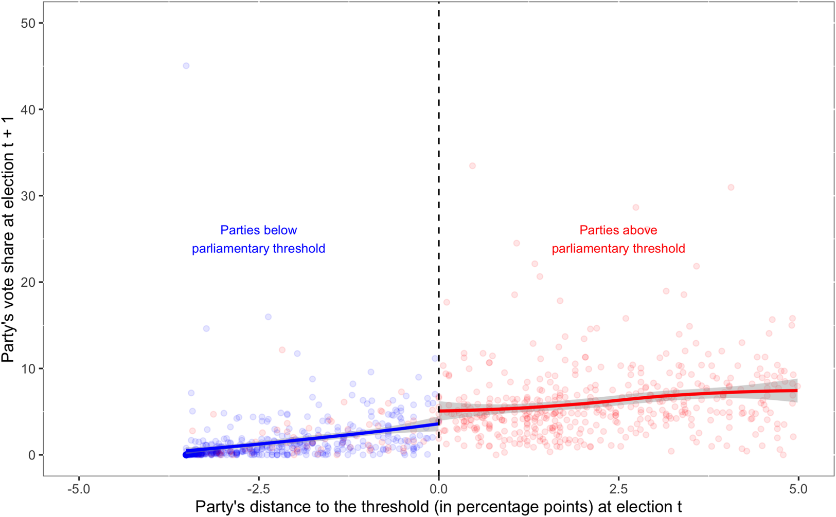
The plot on Figure 1 represents this idea graphically, using raw data from Dinas et al. (Reference Dinas, Riera and Roussias2015).Footnote ⁶ This paper tries to answer a question similar to the one asked by Lee (Reference Lee2001), but in multiparty systems. They want to understand whether the parliamentary representation of small parties makes them more likely to be successful in subsequent elections. In the figure, the x-axis represents the running variable, which determines whether units (parties) fall into the treatment or control group. In this case, that variable is each party's distance to the threshold in election t, in percentage points. For example, if the electoral threshold is one of 5 percentage points and a given party has a vote share of 3, that party will fall 2 percentage points below the threshold – meaning it will have a value of −2 in this variable. The y-axis represents our outcome of interest – the party's vote share in election t + 1 (the following election).Footnote ⁷

Figure 1.

Parliamentary representation and the subsequent success of small parties (example from Dinas et al., Reference Dinas, Riera and Roussias2015).

Notes: Each dot represents one party in an election with a legally fixed electoral threshold in place. Blue dots represent parties that did not enter parliament; red dots represent parties that did enter parliament. Vertical dotted line represents the value of threshold in each country. For more details on these data, please see Dinas et al. (Reference Dinas, Riera and Roussias2015).

In this example, we see that there is a clear positive relation between the forcing variable and the outcome (although that is not necessarily always the case). Our identifying assumption is that, despite this positive relation, the jump in the predicted values at the cutoff (the difference between the leftmost value in the red portion of the function and the rightmost value in the blue portion) identifies our treatment effect – the effect of entering parliament – because other variables that affect the party's subsequent success should not also jump around this value.

Let us now try to put this intuition into a slightly more formal language. We will use capital letters to denote random variables, whose realized values are denoted with lower cases. Imagine an outcome Y, which can take the value y ₁ if the treatment has been assigned, and y ₀ if the treatment has not been assigned. We tend to call Y ₁ and Y ₀, that is, the random variables of which realized values are drawn, as the potential outcome under treatment and control condition respectively, precisely because we remain agnostic as to which of the two treatment conditions has been actually realized. For any given agent i, then, the causal effect, call it τ, is defined as the difference between the two potential outcomes: τ = Y _i1 − Y _i0. Since, however, any i can only be observed either under treatment or under control status at the same point in time, for every i we can only, at the maximum, observe one of the two potential outcomes – the so-called fundamental problem of causal inference (Holland, Reference Holland1986). In the example of Figure 1, this problem means that we can observe a party that got parliamentary representation in the treatment group (the group of parties that enter parliament). But we cannot observe the unrealized potential outcome: the same party had that unit not taken the treatment – that is, had it not been able to enter parliament. To be sure, if there were no heterogeneity in treatment effects—if, that is, units were invariably reacting in the same way to the treatment—the problem would be practically resolved, since we could easily exchange them. We know well, however, that this is not the case. Heterogeneity abounds, from the effect of an aspirin on headaches to the effect of UN peacekeeping forces on conflict termination. We thus need to do something about this.

The standard way to proceed, then, is to move from individual to group-level effects. Again going back to the example on Figure 1, instead of trying to estimate the effect of parliamentary representation on each party separately, we ask if entering the parliament had any effect on average, either considering the whole group or a subset of this group. We typically use the mean to generate such summary estimates of group effects. Thus, we can define and then seek to estimate the following effects:

• • Average treatment effect (ATE): τ = E[Y ₁ − Y ₀];

• • Average treatment effect on the treated (ATT): τ = E[Y ₁ − Y ₀|D = 1];

• • Average treatment effect on the control (ATC): τ = E[Y ₁ − Y ₀|D = 0];

where E denotes the expectation (population average) over the quantity in the brackets. As we will see later on, these groupings are not the only ones available. They are, however, the most intuitive ones to think of. They can be easily decomposed by conditioning further on values of pretreatment variables.

So, now think of an experiment. The way experiments identify the ATE is by random assignment to the treatment, which implies that, in expectation, Y ₁ and Y ₀ are the same for each i precisely because they had no choice to select into treatment. So, the question is now how does the RD identify these effects, if at all?

The RD operates at the margin. It assumes that potential outcomes move continuously in the neighborhood of the treatment. Practically this means that other predictors of the outcome, potentially also affecting treatment status – for example, the party's resources or electoral appeal in the example in Figure 1 – can themselves vary as we move from lower to higher values of the running variable, which is how the variable whose values include the cutoff is known.Footnote ⁸ What is needed is that they vary continuously as we move from marginally below to marginally above the threshold. This is the only assumption needed for the discontinuity design, at least if we are going to estimate the effect at the cutoff point. Known as the continuity assumption, it requires that potential outcomes do not jump but rather move smoothly in the area of the cutoff (c). If this is the case, we identify the effect of parliamentary entry on a party's subsequent electoral success by comparing parties just above the electoral threshold with those just below it:

(1)$$\tau _{{\rm RDD}} = E[ {Y_1-Y_0\vert X = c} ] = E[ {Y_1\vert X = c} ] -E[ {Y_0\vert X = c} ] .$$

The problem of course with 1 is that we cannot observe both Y ₁ and Y ₀ when x = c. At X = c units are either treated or not. Thus, there is no common support to derive $\hat{\tau }$. To gain common support, we need to extrapolate y ₀ from x _i < c to x _i = c. Thus, in practice, what we can realistically aspire to is:

(2)$$\tau _{{\rm RDD}} = \mathop {\lim }\limits_{\Delta \to 0} \{ {E[ {Y_i\vert c < x_i < c + \Delta } ] -E[ {Y_i\vert c-\Delta < x_i < c} ] } \} , \;$$

which implies that as Δ tends to zero, continuity in potential outcomes allows us to construct the missing counterfactual. Now, compare Equation 3 with the expressions of average casual effects shown above. Are we capturing any of them? Not really. Indeed, what this equation recovers is a local effect in the sense that it applies only to those who are at the threshold. This is why the RD recovers a quantity known as the Local Average Treatment Effect (LATE), which may or may not be theoretically useful according to the question one poses. For sure, however, it is better than nothing.

Estimation

Parametric estimation

The question then becomes how to estimate this effect. Since units are either treated or not, exactly at the cutoff c, we cannot simultaneously observe both Y ₁ and Y ₀. Again, we need to impute one of the two. In slightly more formal language, we want to estimate the difference between the rightward limit of the function as the running variable converges to zero and its leftward limit as the running variable converges to zero. We do this by minimally extrapolating at the point of the discontinuity, through the following equation:

(3)$$Y_i = \alpha + \beta ( {X_i-c} ) + \tau D_i + v_i, \;$$

where X _i is the running variable, c represents the cutoff value that is to be found somewhere along the range of values of X and D denotes the treatment status, switching on for units that take the treatment, in this case assigned only if X _i > c. Since X _i is centered at the cutoff, α stands for the average value of Y _i for those with X = c and D = 0. α + τ tap the average value of Y _i for units with X = c and D = 1, and thus τ is the difference between the two: the difference in the expected outcome between treatment and control condition for units with X = c, that is, for those at the cutoff.

Assuming continuity of potential outcomes at the cutoff, this setup allows us to identify the effect of D on Y at that cutoff. Thus, it becomes quite evident that the RD performs quite well in terms of internal validity – the criteria under which the effects are identified are often likely to be met – at the expense of external validity – such effects are only identified at the cutoff and moving away from it requires additional assumptions (Angrist and Rokkanen, Reference Angrist and Rokkanen2015). Yet, Equation 3 imposes some additional and largely unnecessary assumptions, which go beyond what we need to assume for the RD. For example, it assumes that the relationship between X and Y can be approximated by the same functional form, β, both below and above the threshold. We can easily relax this assumption by interacting X and D:

(4)$$Y_i = \alpha + \beta ( {X_i-c} ) + \tau D_i + \gamma D( {X_i-c} ) + u_i$$

Now, we allow units below the cutoff (β) to have a different slope to summarize the relationship between X and Y, than those above (β + γ). Moreover, there is no reason to assume a linear functional form to summarize the link between X and Y. Doing so runs the danger of confusing non-monotone functional forms for jumps, if they are close to the cutoff. We can do this by adding higher polynomials of X. Here is an example with up to four polynomials, which is what Lee's (Reference Lee2001) seminal paper on incumbency advantage estimated:

(5)$$\matrix{ {\matrix{ {Y_i = \alpha + \beta _1( {X_i-c} ) + \tau D_i + \gamma _1D( {X-c} ) + } \cr\!\!\!\!\!\!\!\! {\beta _2{( {X_i-c} ) }^2 + \gamma _2D{( {X-c} ) }^2 + } \cr \!\!\!\!\!\!\!\!{\beta _3{( {X_i-c} ) }^3 + \gamma _3D{( {X-c} ) }^3 + } \cr {\beta _4{( {X_i-c} ) }^4 + \gamma _4D{( {X-c} ) }^4 + w_i} \cr } } & {} \cr } $$

Again, all we are really interested in is τ, which provides the effect of D on Y at X = c. This is of course just one example. The more generic form would be: Y _i = α + f(X _i − c) + τD _i + e _i, which taps any possible function to link X with Y.

Our discussion of estimation starts with the parametric approach because we believe it can be more intuitive for readers unacquainted with the RDD framework. However, as we note in the following section, there has been recent criticism of this approach, which is no longer recommended. Instead, we recommend readers to focus on non-parametric estimation, the estimation of which we outline below.

Fuzzy RD

Thus far we have only considered the following case: a given threshold c deterministically assigns who takes the treatment and who does not. However, in the example from Figure 1 we see that some parties that fail to reach the electoral threshold still manage to enter parliament (red dots left of the dotted vertical line that designates the cutoff). This can be for a number of reasons. For instance, these parties may be part of a coalition which, as a whole, manages to secure a vote share large enough to enter parliament. Such parties take the treatment (parliamentary entry), despite failing to reach the cutoff (electoral threshold). For those familiar with the IV design, this group might already ring a bell. They are the so-called ‘always takers’, that is, units who do take treatment irrespective of which group they are assigned. For these units, being above or below the cutoff c is not anymore informative about their treatment status.

In this case, instead of assigning treatment status deterministically, the cutoff point does so only probabilistically. Parties above the threshold have a higher probability of entering the parliament; but it is not certain that those above the threshold will enter and those below will not enter. Seen in this way, c now becomes an instrument for actual treatment status: crossing it changes the probability of taking the treatment, but does not anymore determine it. In other words, being above or below the cutoff point is not anymore a synonym for treatment status. The two can differ insofar as: (a) there are units that do not take the treatment even if above c (never-takers); (b) there are units that take the treatment even if below c (always-takers); or both (a) and (b). Insofar as c produces a significant gap on the probability of being treated, we can still use it as a way of identifying the effect of treatment on outcome. We do this by applying the so-called fuzzy RD, which combines the logic of a sharp RD (the RD as we had considered it until now, where c determines treatment status) and that of IV. Instead of running Equation 3 for example, we now start by predicting treatment status, D _i, on the basis of the discontinuity on the cutoff:

(6)$$D_i = \alpha + \beta ( {X_i-c} ) + \delta Z_i + v_i$$

where D _i switches on for those in treatment and Z _i is a dummy that turns on for units above cutoff c. We predict $\widehat{{D_i}}$ from Equation 6 and then estimate Y, using the same cutoff but with $\widehat{{D_i}}$ instead of D _i:

(7)$$Y_i = \alpha + \beta ( {X_i-c} ) + \tau \widehat{{D_i}} + v_i$$

As with the sharp RD, the identifying assumption behind the fuzzy RD is the continuity of the potential outcomes at the area of the threshold. Yet, unlike the sharp RD, we now need to make two additional assumptions. The first is that there is first stage, that is, δ ≠ 0. In other words, we expect that crossing the threshold has a non-zero change in the probability of receiving the treatment. As with the IV, this assumption is easy to test empirically, by simply estimating parameters of Equation 6. As with an IV, the stronger the first stage, that is, the sharper the gap between treatment and control at the cutoff, the more efficient (and less biased) the estimates from the second stage are. The second assumption is exclusion. This means that the only way in which crossing the threshold can affect the outcome is via the change in the probability of treatment status. This is a crucial assumption in IV approaches. In fuzzy RDDs, however, it is much more likely to hold insofar as other variables that could also affect the outcome can often be assumed to be continuous around the threshold (i.e., they should not jump).

Snapshot on extensions

We now consider two specific conditions that do not allow for a standard (either sharp or fuzzy) RD but could still be analyzed following the same principle. To start with, imagine a setup where there is an obvious gap between units above and units below threshold, but this jump is blurred due to a heaping of observations very close to the cutoff. When heaping practically makes an otherwise observable gap disappear we can, under conditions, drop observations responsible for this heaping and consider only those right below and above them. Alternatively, imagine that there is sorting taking place right at the cutoff but not slightly away from it. Again, one solution could be to drop observations neighboring the cutoff, and look only at those units less sensitive to such sorting (Eggers et al., Reference Eggers, Fowler, Hainmueller, Hall and Snyder2015). To help visualize this idea, consider again Figure 1, but imagine that we make a hole, symmetrically around the cutoff. We thus end up comparing the observations outside this area, that is, units that do not fall into this hole. Precisely because we end up dropping these observations at the very heart of the RD, this approach is known as donut-RD. For an interesting application, see Barreca et al. (Reference Barreca, Guldi, Lindo and Waddell2011). In general, precisely because this heaping is non-random, one needs to be extremely careful in whether and how to implement this design (Barreca et al., Reference Barreca, Lindo and Waddell2016).

Now, imagine that instead of a gap in the levels of Y _i, the treatment, assigned at cutoff c, generates a systematic jump in the slope that links the running variable with the outcome. In other words, imagine that instead of being interested in the gap in the level of Y _i as a result of D _i, assigned if X _i > c, we are interested in the change in the slope between X _i and Y _i before and after c, which we attribute to D _i. We can do this by running two regressions. First, you regress Y _i on X _i − c and the interaction between X _i − c and a dummy variable denoting observations above the threshold. One can always add more polynomials of X _i − c. You are interested in the coefficient attached to this interaction term, say ϕ. You then replicate this procedure but using D instead of Y _i in the left-hand side of the equation. Call the interaction term from this new equation λ. Then, take the ratio: ϕ/λ. This is often called a regression kink design (Nielsen et al., Reference Nielsen, Sørensen and Taber2010). Interested readers may want to look at Card et al. (Reference Card, Lee, Pei, Weber, Cattaneo and Escanciano2017).

A checklist of tests for studies implementing RD designs

• • Plot the distribution conditional on the distance to the threshold.

Plotting the raw data has become standard practice in RD designs. The researcher should start the presentation of the analyses with a plot of the local averages of the dependent variable, on the y-axis, against the running variable, on the x-axis, along with a fitted line on both sides of the threshold. Providing this plot has a number of attractive advantages. It increases transparency; provides the reader with a sense of how large the discontinuity around the threshold is, as compared to the fluctuation of the dependent variable in regions away from the threshold; allows the reader and researcher to inspect the functional form of the relationship between the dependent and forcing variable at both sides of the cutoff, which can provide guidance in the choice of the appropriate model; and allows one to identify potential outliers (Lee and Lemieux, Reference Lee and Lemieux2010: 284).

In order for these goals to be achieved, the plot should employ a flexible regression model such as a polynomial, as a ways of smoothing the graph. Moreover, the researcher should pay attention to the choice of bin size, which should be wide enough to reduce the noise but narrow enough to allow for the comparison of observations close to the threshold from both sides (Lee and Lemieux, Reference Lee and Lemieux2010: 308–309). Calonico et al. (Reference Calonico, Cattaneo and Titiunik2015) propose a procedure that yields automatic, data-driven plots that can be easily implemented with the rdrobust package. We recommend researchers report this plot.

This being said, the graphical representation represents a necessary, but not sufficient, first step in the presentation of the results of an RD design.

• • Focus on non-parametric models.

As discussed in the previous section, the RD can be estimated using parametric or non-parametric procedures. Recently, however, parametric models have received criticism, since they can lead to noisy estimates (e.g. Gelman and Imbens Reference Gelman and Imbens2019). Given that parametric approaches use the whole sample, they award too much weight to observations far from the threshold. For this reason, we recommend researchers to focus on non-parametric models.

• • Show the results using different bandwidths.

We recommend that researchers report the estimates of non-parametric models at varying bandwidths, both smaller and larger than the optimal one. Ideally, the coefficient will hold regardless of the specific bandwidth size – even if the loss of precision means that, with smaller bandwidths, the results fail to reach statistical significance. Changing the bandwidth can easily be done with software, as we detail in section ‘Software’.

The choice of the specific bandwidths to try should also follow some criteria. Bandwidths that are too large can produce bias in the estimates; while bandwidths that are too small can lead to high variance (Cattaneo et al., Reference Cattaneo, Idrobo and Titiunik2020). As such, it is recommendable that researchers choose bandwidths that are around the optimal one, such as those between half and double the optimal bandwidth.

Our recommendation is that researchers report a plot with a high number of bandwidths within this range. Concretely, researchers may report the bandwidth in the x-axis and the LATE, along with confidence intervals in the y-axis.

• • Run manipulation tests.

One of the key issues with RD designs is the possibility of manipulation of units into the control or treatment group. One way in which such manipulation can happen is self-selection. Consider you are a mayor and your income is higher if the population of your municipality has 5000 people or more. If its actual population is 4980, you have an incentive to slightly misreport it so that your municipality falls just above the threshold.

This problem is called sorting, and it represents a crucial threat to the validity of RDs. A researcher using an RD design to estimate the effect of being above or below the 5000 threshold on some outcome of interest will run into estimation issues in this situation, because one can no longer assume that the only thing that ‘jumps’ around the threshold is the probability of the treatment. For example, consider that only mayors who have a higher underlying propensity to engage in corruption are likely to manipulate the population of their municipality to increase their income. This would mean that more municipalities whose mayors have a propensity for corruption will end just above the threshold than just above it. In this case, the probability of having a mayor with a propensity for corruption also jumps around the threshold. This means that such propensity can confound the relation one is interested in estimating.

Given its importance for RD designs, it has come standard to test for sorting in such designs – even when there is no theoretical reason why one might expect manipulation to occur. An initial check for sorting was proposed by McCrary (Reference McCrary2008). The basic idea is that, in the absence of sorting, the density of the forcing variable should not have a significant discontinuity around the threshold. In other words, there should be no significant jump in the number of units placed just below and just above the threshold. Going back to the example above, if there is no sorting, one should expect a similar number of municipalities to have a population number just below 5000 and a population number just above that value. However, if mayors do misreport their population in order to increase their wages, there might be a discontinuity in the density around the 5000 threshold, with more municipalities clustered above this threshold.

More recently, Cattaneo et al. (Reference Cattaneo, Jansson and Ma2018) propose a different estimator which has a number of advantages. Concretely, it does not require prebinning, and it is grounded on kernel functions that are easily interpretable. We recommend that researchers rely on this approach. As we detail in the section ‘Software’, it is easily implemented using RD packages.

• • Replicate the analyses using placebo outcomes.

As discussed previously, RD designs build on the continuity assumption, according to which ‘the only change, which occurs at the point of discontinuity, is the shift in the treatment status’ (Cuesta and Imai, Reference Cuesta and Imai2016, p. 377). This means that other covariates apart from the treatment status should not have a discontinuity around the threshold. In practice, it is impossible to show that all observables and unobservables fail to jump around the threshold. Still, the researcher should use placebo outcomes to show that important observables do not show the same discontinuities that the dependent variable does. To do so, one would simply replace the outcome variable with those observables.

Examples of typical observables to be used as placebo outcomes include the lagged dependent variable, geographical units such as region or country, and some time variable such as year or month of the observation, whenever applicable. If the analyses are run at the individual level, the researcher may want to include classic sociodemographic variables such as age, gender, or income. None of these covariates should show a significant discontinuity around the threshold.

• • Replicate the analyses using placebo thresholds.

A final test that researchers should conduct is to replicate the analyses using cutoffs other than the actual thresholds that dictate whether units are ascribed to the treatment or control group. The rationale here is that, under the continuity assumption, there should be no jumps in the outcome variable apart from the one around the threshold.

It is advisable to run multiple placebo threshold tests to increase confidence that the researcher has chosen the correct specification.Footnote ⁹ This can be done, for instance, by relocating the cutoff at artificial points at either side of the threshold (De Magalhães et al., Reference De Magalhães, Hangartner, Hirvonen, Meriläinen, Ruiz and Tukiainen2020). Another example is the one proposed by Imbens and Lemieux (Reference Imbens and Lemieux2008). The authors recommend to run a placebo analysis using the median value of the forcing variable in the treatment group and in the control group. Running the analyses around the median increases the statistical power and makes it more likely to find an effect. Since we expect to find no effect, increasing the statistical power makes the test more conservative.

• • Effect heterogeneity needs caution.

Imagine you conduct a randomized experiment, estimate the ATE and want to see whether its magnitude varies across subgroups. In particular, imagine that you have a reason to believe that the treatment effect will vary by a given factor, say respondent's education level. To be even more specific, imagine all you are interested in is whether the effect is different for those who hold a university degree compared to those who do not. How do you proceed? Typically, you would interact the treatment indicator with a dummy switching on for university degree holders. And how would you then know for sure that it is education rather than some other characteristic that operates as a moderator of the treatment effects and also varies across the two groups, with and without university degree (say, e.g. socioeconomic background)? Well, then you add all such covariates in the same regression equation, interacting them also with treatment status (see e.g. Dinas et al., Reference Dinas, Fouka and Schläpfer2021).

The problem in the RD is that this simple logic does not hold, unless we make additional assumptions about how the forcing variable and the outcome are related. If this link varies across subgroups, for example, between those with and without a university degree, the approach may no longer be valid. In particular, the method severely over-rejects under model misspecification even if researchers only use observations close to the cut-off of the running variable for estimation (Hsu and Shen, Reference Hsu and Shen2019). One could still split sample across combinations of covariates, for example, within university holders coming from low socioeconomic status, but then the dimensionality curse kicks in, which in the RD world is bound to lead to small-n problems.

One recent development in the RD literature tries to address this exact problem by relying on propensity score weighting, in the spirit of Abadie (Reference Abadie2005). Practically, this means weighting observations of one subgroup inversely to the propensity to belong to this group on the basis of a set of covariates. Doing so generates two groups who differ in the moderator but are similar in their weighted propensity to belong to each of the subgroups, based on observables (Gerardino et al., Reference Gerardino, Litschig and Pomeranz2017). Once these weights are applied, each subgroup-specific analysis can then be implemented. See more detailed description of the design in Gerardino et al. (Reference Gerardino, Litschig and Pomeranz2017) and Hsu and Shen (Reference Hsu and Shen2019), who also offer a Stata module, rddsga, to conduct subgroup analysis within the RD setup (Carril et al., Reference Carril, Cazor, Paula Gerardino, Litschig and Pomeranz2017).

Software

As mentioned above, we recommend that researchers focus on non-parametric RDs. This being said, should they want to run parametric RD designs, these can be implemented without the need for specific packages, as they are standard OLS regressions. The researcher can simply regress the outcome on the forcing variable, the treatment variable, and the interaction therein. Should they want to include higher-order polynomials, they can simply add the squared forcing variable and its interaction with the treatment variable. The researcher can then follow the same logic up to as many polynomials as they would like to include in the model.

When it comes to the implementation of non-parametric RDs, available packages make the implementation very straightforward, both in Stata and in R. We recommend the use of the rdrobust package for R and Stata (Calonico et al., Reference Calonico, Cattaneo and Titiunik2014b; Calonico et al., Reference Calonico, Cattaneo, Farrell and Titiunik2017).

The rdrobust package implements RDs using robust bias-corrected confidence intervals, as proposed by Calonico et al. (Reference Calonico, Cattaneo and Titiunik2014a). The main command is rdrobust, the output of which provides the results from three different procedures (which can be accessed via the option ‘all’): conventional, bias-corrected, and robust. As recommended by Cattaneo et al. (Reference Cattaneo, Idrobo and Titiunik2020), researchers should report the conventional point estimate along with the confidence intervals obtained from robust procedures.

rdrobust automatically calculates the optimal bandwidth, but the command provides an option for the user to change it if so they desire. This allows the researcher to show how the findings change as they move around the bandwidth. This package also allows the user to make data-driven plots by using the command rdplot (although researchers can prefer to produce their own plots); and to estimate the density of units near the cutoff using the command rddensity (Cattaneo et al., Reference Cattaneo, Jansson and Ma2018). Finally, the package implements both sharp and fuzzy RD designs. The default is a sharp RD, but the user can specify a fuzzy RD by using the option ‘fuzzy’ and indicating the treatment variable in parentheses.

Electoral victory thresholds

Voting is the quintessential political action. For this reason, it may come as no surprise that one of the most commonly RD designs used in political science is the discontinuity produced by electoral results. The vote share of a given party is continuous and researchers can use the jump around the threshold of victory (usually 50% of the vote) to estimate the effect of such victory on outcomes of interest.

The original application of this design is the introductory example: the paper by Lee (Reference Lee2001) that estimates the effect of the so-called incumbency advantage. Despite long-standing discussion of how elected US politicians were more likely to be re-elected, this effect is hard to estimate empirically because incumbents are likely to differ from challengers in a number of characteristics. Their victory in the previous election may have been caused by their higher amount of resources, higher debate skills, or more appealing policy platform. The author overcomes these endogeneity issues by exploiting the discontinuity generated by narrow electoral wins. Using an RD design, the paper shows that narrowly winning an election at time t is associated with a higher probability of winning at time t + 1. The causal effect is as large as 40–45 percentage points.

A first set of studies has provided further detail on the incumbency advantage. Trounstine (Reference Trounstine2011) shows that the incumbency advantage extends to local American politics as well. Butler (Reference Butler2009) shows that the incumbency advantage is more pronounced for non-freshmen incumbents than it is for freshmen ones. Looking into the effect in other regions of the globe, Hainmueller and Kern (Reference Hainmueller and Kern2008) show incumbency to have spillover effects in mixed systems – concretely, the one in Germany. Uppal (Reference Uppal2009) finds the opposite effect in Indian State legislative elections. Incumbents seem to actually be disadvantaged when it comes to assuring their reelection.

Another set of studies has used this design to look at the effect of electoral victory on the behavior of political elites. For example, Thompson (Reference Thompson2020) looks at whether local-level law enforcement differs based on the party in power. Looking into the effect of compliance with federal requests to detain unauthorized migrants under the Trump administration, the author finds no evidence that Democratic sheriffs are less likely to comply than are Republican ones. In turn, Ruipérez Núñez and Dinas (Reference Ruipérez Núñez and Dinas2020) use this design to show the political use of public memory in post-authoritarian Spain. They show that municipalities where the right narrowly wins are significantly more likely to keep street names allusive to the right-wing dictator Franco; while municipalities where the left narrowly wins are significantly more likely to remove them. Finally, Huidobro and Falcó-Gimenez (Reference Huidobro and Falcó-Gimenez2020) use this design to show that women and young leaders narrowly winning municipal elections in Spain are significantly less likely to be appointed mayors than their male and older counterparts.

Another example of uses of this design is the literature that has looked at the monetary and non-monetary returns to holding office. Eggers and Hainmueller (Reference Eggers and Hainmueller2009) show that holding office can significantly affect wealth. Narrowly winning an election to become a UK MP almost doubles the wealth of Conservative MPs – although they find no such effect when drawing upon MPs for the Labour Party. Further research has suggested that there are non-monetary benefits to holding office as well. Using data from close US gubernatorial races in the post-war period, Barfort and Klemmensen (Reference Barfort and Klemmensen2017) show that hold office causes an increase in life expectancy of around 5 years.

A final example is the use of such designs to identify the effect of the success of different parties on policies. Lee et al. (Reference Lee, Moretti and Butler2004) find no evidence that the strength of electoral support to a candidate affects the moderation of their policies. Benedictis-Kessner and Warshaw (Reference Benedictis-Kessner and Warshaw2016) find that narrowly elected democratic mayors increase the expenditures of that municipality. Along similar lines, Benedictis-Kessner and Warshaw (Reference Benedictis-Kessner and Warshaw2020) find narrowly electing a Democrat legislator to US county governments increases public expenditure by 5%.

Fixed parliamentary thresholds

Many countries around the world have legally fixed electoral thresholds, such that only parties making it across such thresholds are granted parliamentary representation. These thresholds bring about a ‘jump’ in the probability of a party entering parliament, which researchers can exploit to estimate the effect of parliamentary representation on a number of outcomes of interest.

In the initial application of this design, Dinas et al. (Reference Dinas, Riera and Roussias2015) study the effect of parliamentary representation in the survival of small parties. Using data from all countries around the globe that include an electoral threshold, the authors find that narrowly making it across the electoral threshold increases the vote share for a given party in the following election – an effect size that the authors estimate at around two percentage points.

Dinas and Foos (Reference Dinas and Foos2017) use a similar design to look into the effect of local politics on national-level success. The authors look into the case of Germany, where state elections include an electoral threshold and elections at different levels are not coordinated. Their analyses show that narrowly making it across the electoral threshold in a state election increases the subsequent national-level success of a party. The effect, however, is limited to observations when the gap between state and national elections is above the median – giving the party time to use its newly acquired organizational resources.

Another strand of research has used similar designs to look into how the parliamentary representation of parties of a given family affects the remaining ones. For example, Abou-Chadi and Krause (Reference Abou-Chadi and Krause2018) study the effect of the parliamentary representation of radical-right parties on the policy positions of the remaining parties. They find that such representation makes the remaining parties adopt more anti-immigrant policy positions – an effect that extends both parties of the mainstream right and the mainstream left. In turn, Bischof and Wagner (Reference Bischof and Wagner2019) use this design to show that the parliamentary presence of a radical-right party – but not that of a radical-left party – polarizes the electorate. Finally, using the proportion of the official vote for a party that is reported in post-electoral surveys as an outcome variable, Valentim (Reference Valentim2021) uses a similar design to show that the parliamentary representation of the radical right normalizes the expression of radical-right support.

In an extension of these designs, Valentim and Dinas (Reference Valentim and Dinas2020) extend this logic from the party-level to the party-system level, using the variation created by electoral thresholds as an instrument for the overall level of party-system fragmentation in a given election. In so doing, they find no evidence that party-system fragmentation affects a large number of democratic outcomes.

Population thresholds

Another frequent RD design is the one that draws upon population thresholds. Many countries have rules that apply only to regions whose population is higher than a given threshold. This allows researchers to identify the effect of being under rule, by comparing regions whose populations are just above the threshold to those whose populations are just below them.

A first strand of research has looked into such discontinuities to estimate the effect of different electoral and democratic rules. Fujiwara (Reference Fujiwara2011) uses one such design to empirically test Duverger's Law, according to which proportional systems increase the number of parties running. Taking advantage of the fact that, in Brazil, elections in municipalities with more than 200,000 registered voters employ dual-ballot while smaller ones employ single-ballot pluralities, the author finds that dual-ballot decreases voting for the two better placed candidates. Taking advantage of a similar law in France, Eggers (Reference Eggers2015) identifies the effect of PR on turnout, which the author estimates as being 1–1.5 percentage points. In their study of electoral systems and clientelism, Pellicer and Wegner (Reference Pellicer and Wegner2013) exploit a similar threshold in Morocco. They find that clientelistic parties do worse (winning about half the seats) in PR than in plurality systems. In turn, Campa (Reference Campa2011) looks into gender quotas that are mandatory for Spanish municipalities with more than 5000 inhabitants. Such quotas increase the percentage of elected female politicians by 4–6 percentage points, but seem to have no effect on the policies undertaken by the municipality. Hopkins (Reference Hopkins2011) studies the effect of introducing Spanish-language ballots in elections in the US by comparing counties above and below the legally fixed thresholds above which counties are supposed to offer ballots in different languages. The author finds that Spanish-language ballots increase turnout among citizens with low English skills, and decreased support for ending bilingual education. Finally, Sanz (Reference Sanz2019) takes advantage of the fact that, in Spain, municipalities with less than 100 inhabitants employ direct democracy to study the effect of this form of government on the size of the public sector. The author's findings show that direct democracy significantly reduces both spending and revenues.

Another strand of research has used similar discontinuities to look at the effect of politicians’ wages and resource transfers. Gagliarducci and Nannicini (Reference Gagliarducci and Nannicini2013) exploit population discontinuities that dictate politicians’ wages in Italian municipal governments, to estimate the effect of wages on the performance of politicians. They find that increasing wages causes candidates to be more educated and reduce tariffs, taxes, personnel and other expenditures. Following the same reasoning, De Benedetto and De Paola (Reference De Benedetto and De Paola2014) use these discontinuities as an instrument for politician quality, and find that higher quality politicians increase turnout by about 2 percentage points. In turn, Brollo et al. (Reference Brollo, Nannicini, Perotti and Tabellini2013) study the effect of revenues on political corruption, using population thresholds that dictate the amount of federal transfers to Brazilian municipal governments. They find that increasing transfers by 10% increases measures of corruption by 5–7 percentage points. It also reduces the quality of challenger candidates, as proxied by their level of education.

Researchers using these designs should pay attention to two main pitfalls (Eggers et al., Reference Eggers, Freier, Grembi and Nannicini2018). The first one is sorting. As alluded to in section ‘A checklist of tests for studies implementing RD designs’, public officials in municipalities near the threshold may try to manipulate official statistics so that they fall on the side of the threshold that yields the most benefits. The second one is compound treatment arising from the fact that often the same population threshold is used to determine several policies. Eggers et al. (Reference Eggers, Freier, Grembi and Nannicini2018) suggest a number of strategies to deal with these issues. To deal with sorting, one can introduce controls for potential confounding variables. Another possibility is to run donut RDDs that ignore data just around the threshold – where sorting is more likely to take place. Finally, they also suggest that researchers can employ difference-in-RDD designs to try and understand the magnitude of sorting by comparing periods when the treatment is given to units above the threshold to previous periods when that does not occur. To deal with compound treatment effect, one possibility is to just assume that the design is not identifying the effect of a single policy, but of multiple ones. In some cases, a researcher may be in position to make the assumption that the confounding treatments do not affect the outcome, allowing them to identify its isolated effect. Another possibility is to look at the difference between the setting one is studying and other settings where the discontinuities dictate exposure to the confounding treatments, but not to the main one.

Age discontinuities

Another classic RD design exploits discontinuities generated by someone's date of birth. This is especially pertinent in the identification of the effects of early voting experiences. Citizens in democratic countries are allowed to vote when they reach the legally fixed age, which creates discontinuities between individuals who were narrowly too young to vote and those who had just turned old enough to vote.

Researchers have looked into such discontinuities to identify the effect of the habit-formation nature of voting. Meredith (Reference Meredith2009) finds that past eligibility significantly affects the downstream probability of voting and partisan identification, an effect that persists for several future elections. Similarly, Coppock and Green (Reference Coppock and Green2016) use a number of such discontinuities to look at the habit-formation nature of voter turnout. They find that , when compared to narrowly non-eligibles, individuals narrowly eligible to vote at time t were more likely to vote at time t + 1. Schulte-Cloos (Reference Schulte-Cloos2019) uses a similar discontinuity to identify the effect of being first eligible to vote for a European parliament election on subsequent political interest and closeness to challenger parties. Unlike what previous research feared, she finds a positive effect in interest and no evidence of increasing closeness to radical-right parties. Extending the effects of voting to other members of the voter's household, Dahlgaard (Reference Dahlgaard2018) uses data from four municipal elections in Denmark and finds that parenting a newly enfranchised voter increases the likelihood of voting by almost 3 percentage points.

Spatial discontinuities

Regression discontinuities can also be done using space. Sometimes geographical lines demarcates whether units are exposed to a given treatment or not. If the continuity assumption holds – meaning that there should be no other ‘jump’ around this line apart from the jump in the probability of receiving the treatment – researchers can use this line in a RD design.

One example is the use of war lines in conflict areas. For example, Tur-Prats and Valencia Caicedo (Reference Tur-Prats and Valencia Caicedo2020) employ a RD along the Aragon front in the Spanish Civil War to show that political violence during that war significantly reduced generalized trust. Fontana et al. (Reference Fontana, Nannicini and Tabellini2018) use a discontinuity along the Gothic line, a battlefront in Italy, north of which violence and Nazi occupation during WWII lasted longer. They show that the experience of such violence and occupation increased voting for the Italian Communist party in the post-war period.

Other studies have used discontinuities generated by the limits of reachability of some technology. For example, Gonzalez (Reference Gonzalez2021) exploits the limit of phone coverage as a threshold to identify the effect of cell phone coverage on electoral fraud. He finds that such coverage decreases fraud. A set of additional analyses suggest that this is due to cell phone coverage allowing for social monitoring. Adena et al. (Reference Adena, Enikolopov, Petrova and Voth2020) use a spatial RD to study the effect of bombings during World War II. They use discontinuities generated by the effective range of US bombers and find that bombing significantly increased resistance activity.

A final set of examples are lines generated by borders and administrative regions. Holbein et al. (Reference Holbein, Schafer and Dickinson2019) use a spatial RD to identify the effect of lack of sleep. The cutoff are different time zones, which decrease the sleep needs of individuals living very close to the Eastern border of time zone lines, who sleep significantly less than those close to the Western border. They find that sleep deprivation decreases a number of pro-social behaviors, among which voting. Ferwerda and Miller (Reference Ferwerda and Miller2014) are interested in whether political devolution to native powers increases resistance to occupation by foreign powers. Their spatial RD is based on the border of the Vichy line in France, which assigned municipalities into Vichy rule or German rule between 1942 and 1944. They find that the municipalities in the vicinity of the border, but on the Vichy side – which had enjoyed political devolution – witnessed significantly lower levels of resistance.