

INTRODUCTION
The foreseeable expansion in agriculture could lead to global environmental change and unprecedented loss of biodiversity and ecosystem services (Tilman et al. 2001; Foley et al. Reference Foley, Ramankutty, Brauman, Cassidy, Gerber, Johnston, Mueller, O'Connell, Ray, West, Balzer, Bennett, Carpenter, Hill, Monfreda, Polasky, Rockstrom, Sheehan, Siebert, Tilman and Zaks2011). These competing demands result in poorly understood and sometimes unresolvable trade-offs between conservation and economic development (Sandker et al. 2012). Reconciling agriculture, conservation and other competing land uses partly requires that we finely analyse these demands on land availability at the landscape scale (Sayer et al. 2013). The landscape is perceived as an object at an intermediate level of organization (1 km2 or more), which is often easier to manage than that of whole ecosystems (Shoute et al. 1994; Twery 2004). The landscape mosaic of agriculture fields and forests also results from individual decisions by farmers and other stakeholders who integrate biophysical and social constraints in their decision-making processes (Leach et al. 1999; Garcia et al. Reference Garcia, Shonil, Bhagwat, Ghazoul, Cheryl, Nanaya, Chepudira, Kushalappa, Nasi and Vaast2010). Landscape modelling may help to formulate, test and validate hypotheses, often in the spatial and temporal dimensions that are impossible to recreate and validate with in situ experiments (Baker Reference Baker1989; Baker et al. Reference Baker, Egbert and Frazier1991; Mladenoff & Baker 1999; Gaucherel & Houet 2009). However, even recent models have failed to capture the highly complex nature of these systems involving multiple stakeholders and environmental factors, multiscale processes and multilevel dynamics (Burel & Baudry Reference Burel and Baudry2003; Gaucherel & Houet 2009). For these reasons, we aimed to develop a model of land-use changes and to illustrate it at a specific site.
The Western Ghats of India offer an ideal opportunity to understand trade-offs between conservation and development in a crowded space. The district of Kodagu (state of Karnataka) has a human density that is now twice what it was 1950 (Guilmoto 2000) and now produces 2% of the world's coffee, yet still harbours tigers and elephants in its forests and agroforests (Garcia et al. 2007). From 1977 to 2007, forest cover declined by 30% in Kodagu, while the area under coffee plantation doubled, as in some other tropical areas (Steffan-Dewenter et al. 2007; Sandker et al. 2012; Jha et al. 2014). Coffee in the district is produced under canopy cover, sheltering a large biodiversity (Garcia et al. Reference Garcia, Shonil, Bhagwat, Ghazoul, Cheryl, Nanaya, Chepudira, Kushalappa, Nasi and Vaast2010); however, agricultural intensification leading to the removal of shade trees or the modification of the canopy cover has raised concerns about the area and the sustainability of the farming practices (Nath et al. 2011), as it has at larger scales (De Beenhouwer et al. Reference De Beenhouwer, Aerts and Honnay2013). The rice paddies, which constitute approximately a third of the landscape area, are also under pressure and are progressively being abandoned due to low market prices and shortages of labour (Ambinakudige & Choi Reference Ambinakudige and Choi2009). Terraced rice fields and the coffee plantations are part of the same production system and should be integrated into a comprehensive landscape model.
Process-explicit models are particularly appropriate for highlighting realistic changes in land use and land cover due to various anthropogenic or natural ecological processes (Costanza & Voinov Reference Costanza and Voinov2003; Gaucherel et al. 2010). Yet existing models rarely take into account several levels of organization; at best, models so far have considered landscapes with only one decision unit (i.e. a single farm) (Castellazzi et al. Reference Castellazzi, Matthews, Wood, Burgess, Conrad and Perry2007; Houet et al. 2009). We used the free, open source Dynamic Patchy Landscape (DYPAL) modelling platform and its formal grammar framework (Gaucherel et al. 2012; Houet et al. 2014) to address two interlinked issues in the village of Kottoli (Kodagu). Firstly, based on an understanding of past and present dynamics, it tests the hypothesis that, as in most anthropogenic landscapes (Houet et al. 2009; Houet et al. 2014), dynamics in Kottoli are driven by farmer decisions, instead of by independent patch dynamics such as cereal rotations on isolated patches or autonomous fallow environments (rice fields and coffee plantation blocks are assumed to be homogeneous in the model). The landscape dynamics observed in India will be compared with findings on land use in coffee landscapes elsewhere in the world (Steffan-Dewenter et al. 2007; Ellis et al. Reference Ellis, Baerenklau, Marcos-Martinez and Chavez2010; Godfray et al. 2010; Sandker et al. 2012; Hylander et al. 2013; Jha et al. 2014). Secondly, we explore the sustainability of the Kottoli landscape by defining prospective scenarios and simulating future dynamics.
METHODS
Study area and farmer typology
Since the introduction of coffee in India in 1834 by the British, coffee plantations have expanded, replacing the original vegetation cover, first in the moist deciduous forests and then in the wet evergreen forests (Appendix S1 & Table S1) (available online). This expansion took place primarily in privately controlled forested lands, while state-controlled forests have remained largely untouched (Garcia et al. Reference Garcia, Shonil, Bhagwat, Ghazoul, Cheryl, Nanaya, Chepudira, Kushalappa, Nasi and Vaast2010). Today, native trees are being replaced by Grevillea robusta sp. (Australian silver oak), a fast-growing species that is also used as a shade tree in coffee plantations. The use of irrigation to induce flowering also impacts the management of the canopy as the trees can obstruct sprinkler irrigation. A farmer opting for irrigation will thus consider reducing the density of trees in his or her block (Chretien & Descroix 2007). Coffee cultivation has increased in the past 20 years and has been associated with rising living standards and labour costs, which have led to the shrinkage of the area under rice cultivation (Ambinakudige & Choi Reference Ambinakudige and Choi2009). Rice used to be the dominant crop in Kodagu, but is now declining (Moppert 2005) (Fig. S1).
Past land-use maps of the Kottoli village were available. We used semi-structured interviews (43 farmers in depth, and 126 in total; Appendix S1) to examine the past and present management practices of the farmers (Bierschenk & Olivier de Sardan Reference Bierschenk and Olivier de Sardan1997; Olivier de Sardan 2003) and to define a farm typology of the village through a principal components analysis (Bidogeza et al. Reference Bidogeza, Berentsen, Graaff and Oude Lansink2009; Tittonell et al. 2010) and a hierarchical ascendant classification (Appendix S1 & Table S2).
Simulations
We modelled the Kottoli landscape with the DYPAL modelling platform (Appendix S2), which seems uniquely able to rigorously handle such multiscale and non-stationary (i.e. with rupture dynamics) landscapes (Gaucherel et al. 2010; Houet et al. 2014). To assess the model's validity, DYPAL-simulated maps (10 replicates each) were compared in terms of land cover composition and spatial configuration with the 2011 map of Kottoli. We used three computations to compare simulated and observed configurations at successive scales – multiscale heterogeneity map (MHM) and comparison map profile (CMP) spatial analyses (Appendix S3) – and the Wilcoxon rank-sum test to globally confirm these. We first computed land-cover connectivity (contagion) maps of Kottoli simulations and observations with the MHM software (Gaucherel 2007). Simulated connectivity maps were then compared to the 2011 map on the basis of a distance index, computed as averaged differences of absolute values and the Pearson cross-correlation for relative variations (Gaucherel et al. 2008). Once the simulations were validated, and in order to understand the differential success of various land covers (forest, silver oak and fallow), we computed land-cover multiscale density maps with the MHM software and compared them to the corresponding observed density maps with the CMP software.
Three additional conditions on landscape driving rules were implemented in order to further elaborate the model:
-
(i) Timelines and disruptive (non-Markovian) events (with 5-year time step simulations): based on analysis of the interviews, coupled with trends that were visible in the ages of the plantations, we identified the following events: 1950 (first coffee plantations in Kottoli), 1970 (introduction of silver oak and fertilizers), 1985 (the ‘coffee boom’) and 2000 (increase in living standards leading to higher labour wages for paddy cultivation).
-
(ii) Conditions of neighbouring patches for paddy conversion: for the purposes of the present maps, virtually all converted terraces (99.5%) were connected to wooded areas or coffee estates, either directly or through another converted terrace. We therefore imposed a connectivity condition (neighbourhood link) on the possible conversion from rice to coffee.
-
(iii) Farm affiliation: each group of farmers had its own strategies and agronomical automaton (i.e. agricultural successions). Hence, each rule was associated with specific probabilities and specific starting dates depending on the farm group.
The simplest DYPAL simulation/hypothesis of Kottoli (H0) consisted of the 18 rules without any landscape-related conditions except the constraint on final area proportions, thus directly assuming multilevel functioning. The final simulation/hypothesis (Hf) took into account the three previous conditions. Improvements in terms of reliability and goodness of fit of the simulations were assessed according to the spatial analyses previously presented.
Prospective scenarios
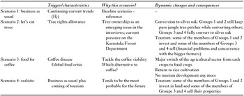
It was our intention to explore with DYPAL possibly contrasting yet socially relevant prospective scenarios that would emerge out of interviews with the stakeholders. An initial scoping exercise was conducted based on a territorial prospective analysis (Leroy et al. 2011), which identified three main drivers of landscape dynamics in Kodagu and some other tropical agroforested landscapes (Ellis et al. Reference Ellis, Baerenklau, Marcos-Martinez and Chavez2010; Sandker et al. 2012; Sassen et al. 2013; Schmitt-Harsh 2013): the structure of land tenure and particularly tree ownership rights, the coffee market and tourism. The alternative scenarios were identified on the basis of the interviews, where respondents would express their possible responses to a coffee crisis.
Scenarios had equal chances of being realized, but we lacked information with which to assess their relative robustness. Scenario 1 – the continuation of the current trends (business as usual) – served as a reference. Scenarios 2 and 3 explored two possible major events disrupting the status quo: the restitution of tree rights to farmers (Scenario 2); and a coffee crisis due to a disease wiping out coffee cultivation or leading to a fall in price (Scenario 3). Scenario 4 explored the development of tourism, seen as probable by our contacts. These four scenarios were then used to define sets of parameters and alternative timelines that were fed into the DYPAL Kottoli model.
RESULTS
Landscape dynamics in Kottoli
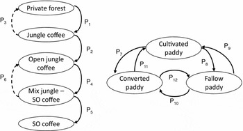
The automata used to describe the dynamics of the agroforestry patches and the rice fields were largely independent (Fig. 1). Interviews showed that highland coffee and lowland paddies never permuted in the landscape. Simulations were developed with the forested land automata for the transition of private forests to a pure silver oak coffee plantation landscape over 70 years through the following successive stages (Fig. 2): private forest patches from which the understory was removed; coffee planted in its place (‘jungle coffee’) for which the canopy cover was reduced to below 75% of its original size (open jungle coffee); and silver oak was then introduced (‘mixed jungle coffee’ and/or ‘silver oak coffee’) replacing harvested or dead jungle trees (‘pure silver oak coffee’). There was no way back from the open jungle coffee plantation to the jungle coffee plantation, although rules having probabilities P3 and P6 seldom occurred (Fig. 1, dashed arrows).
Exhaustive automata and associated rules and probabilities of the Kottoli dynamics. The various states of the patch land covers are the node (ellipses), while the arrows represent transitions between these states. On the left-hand side is the forested land automaton, while on the right-hand side is the paddies automaton (the less frequent transitions – dashed arrows – have an estimated probability to occur of lower than 3%). These automata have been deduced from interviews and may be truncated for certain events (see Fig. S2). SO = Silver oak.

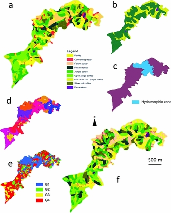
Maps of Kottoli village. (a) Observed map – 2011; (b) initial map – 1950; (c) hydrological layer (in blue, hydromorphic soils close to the main river with no paddy conversion taking place in lowlands); (d) reference points (white) and corresponding areas used in the simulations to locate farms (see Appendix S1); (e) farm typology (blue: group 1, green: group 2, yellow: group 3, red: group 4); (f) simulated map – 2010 with the Hf simulation (same land-cover typology as the initial map).

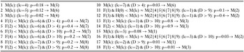
The rice cultivation automaton led to a continuation of rice cultivation or its abandonment, either to fallows or to other crops through conversion, with the latter being non-reversible, as farmers need to invest substantial amounts of cash in order to convert the rice fields. From these two automata, 18 ‘rotation’ rules were extracted (Table 1) and written according to DYPAL's formal grammar syntax (Appendix S2). Finally, each group of farmers as identified by the typology followed truncated versions of both the automata in order to reflect their specific strategies (Fig. 2 & Fig. S2). Group 1 farmers could roll out the whole automaton thanks to their significant capital. For the rice cultivation automaton, Groups 2 and 3 would only let their rice fields remain fallow or convert them, respectively, while Group 4 continued to cultivate rice. For the forest automaton, Groups 3 and 4 entered the silver oak plantation phase at a later point in time.
Formal grammar equations of the corresponding driving rules used in the DYPAL model for the Hf simulation.

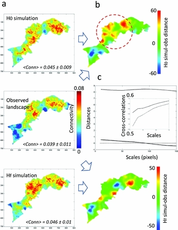
Simulated connectivity maps were in good agreement on average with the observed connectivity map (Fig. 3(a)), although simulated connectivity (0.045 ± 0.01) appeared significantly greater (p-value < 10–5) than what was observed (0.039 ± 0.01; Fig. 3(c)). Distance indices (8.33 ± 0.1 and 0.07 ± 0.34) and cross-correlation indices (0.54 ± 0.03 and 0.57 ± 0.015) validated both the H0 and Hf simulations, respectively. The distance and correlation values were relatively high, considering that they averaged a large number of moving window and image values. However, these agreements were not uniformly spread over the landscape, and the analyses precisely located the places and scales at which the model performed well (Fig. 3(b)). For example, the Hf simulation showed an almost zero distance from the observed landscape, but this value hid an averaged compensation of positive and negative distances at various village places. The H0 simulation showed a higher averaged distance, particularly in the middle of the village (Fig. 3(b), red circle). Cross-correlations, by focusing more on variations in connectivity structures, confirmed these validations, with higher correlations at higher scales (Fig. 3(c)).
Comparisons between the simulated and the observed landscape connectivity (contagion) maps of Kottoli in 2012. The three connectivity maps computed with MHM for observed and simulated values (a, column) are compared to their respective multiscale CMP distance maps (b, up and down) and profiles (c). Colour scales indicate connectivity intensity (named Conn) of between 0 and 0.08 (a) and distances between –50/60 and +50/60 (b). Distance and correlation profiles computed for spatial scales ranging from 10 to 150 are given for H0 (dashed lines) and Hf (plain lines).

The correlation profiles between Kottoli simulations and the observations (Fig. S3) showed that, when accounting for the spatial distribution of land covers with MHM and CMP, the fallow rice field was the best simulated land cover (r² = 0.498 ± 0.025), followed by the silver oak coffee plantation (r² = 0.216 ± 0.041) and forest (r² = 0.099 ± 0.032; Fig. S3(c)). Fallow and silver oak matching were partially due to the absence of both land covers in the southern part of the village (Fig. S3(b)). In the north, the extent and location of fallows and, to a certain degree, silver oak were correctly simulated compared to observations. Only Group 1 and Group 2 farmers (in the north) could let their paddies remain fallow and convert their plantation from jungle tree canopy cover to silver oak canopy cover. Fallow correlations increase (while silver oak correlations decrease) with scale (Fig. S3(c)), thus indicating that the simulations are statistically correct (while the silver oak simulations are incorrect), but locally false (while the silver oak simulations are locally exact). We thus produced relevant and plausible narratives of landscape dynamics, rather than realistic, perfectly fitting simulations. Furthermore, the forest land cover exhibits a comparable scale related to its averaged patch size (approximately 40 pixels or 300 m; Fig. S3(c)).
Future scenarios
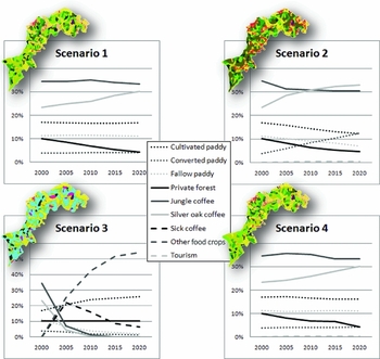
All scenarios pointed to an increase in the conversion of rice fields, and of at least half the remnant private forests, into coffee plantations (Table 2 & Fig. 4). However, in Scenario 3, where the spread of a coffee disease decimated coffee cultivation, conversion of rice fields (to food crops other than rice) was reduced, as was conversion to fallow land. Scenarios 1, 2 and 4 exhibit a decrease in jungle coffee plantation (–3%, –13% and –3%, respectively) in favour of silver oak coffee plantation (+30% for the three scenarios). Fallow rice fields decreased in Scenarios 2 and 3 (–63% and –82%, respectively), but remained stable in Scenarios 1 and 4. Scenarios 1 and 4 were similar to each other in outputs, the only difference being an increase in converted rice fields in Scenario 4 (+16% compared to +9%).
Summarized descriptions of the projected scenarios to be read in conjunction with the previously listed rules (the rules remained unchanged, but were implemented differently in the different scenarios).

Land-cover changes in terms of area proportions (percentages) during the course of the four future scenarios (years 2000–2020; see text for their definitions). An example of the final step (2020) of each scenario is inserted and is displayed with the same colour scale as in Fig. 2.

DISCUSSION
Landscape processes
The DYPAL modelling platform and its associated mathematical formalism succeeded reasonably well in capturing the structure and dynamics of Kottoli, considering that it is difficult to define the DYPAL model, control it and to compare its results. In building this model, we tried to control the main drivers identified in the studied agroforest, ranging from global drivers such as the world market to local drivers such as land tenure and agricultural development policies. Studies in other areas mention additional drivers such as regional climate on the one hand and livelihood practices, local changes in settlements and demographic trends on the other (Ellis et al. Reference Ellis, Baerenklau, Marcos-Martinez and Chavez2010; Hylander et al. 2013; Sassen et al. 2013; Schmitt-Harsh 2013; Tadesse et al. 2014). The latter drivers seem to play a weaker role in Kottoli. The model developed here aimed at differentiating the respective weights of each driver in order to ultimately help formulate effective strategies in landscape management.
Local and multiscale distances and cross-correlation maps confirmed the overall adequacy of the most realistic (Hf) simulation more efficiently than classical similarity indices (e.g. receiver operator characteristic–areas under the curve). According to CMP maps, the averaged distance (0.07 ± 0.34) and the averaged cross-correlation (0.57 ± 0.015) were good, and even improved at larger scales. This was expected, as DYPAL simulates with better accuracy broad patch allocation, rather than the exact land cover for a given patch. These landscape dynamics could now be presented to villagers and stakeholders.
The landscape modelling we have presented here answered our first question that related to the past and present complex multilevel landscape dynamics driven by farmer decisions. Other patchy landscape models that have been developed so far usually neglect multilevel organization and/or reduce it to a single farm type and agricultural production system (Castellazzi et al. Reference Castellazzi, Matthews, Wood, Burgess, Conrad and Perry2007; Gaucherel et al. 2010). Furthermore, most landscape models still use grid-based spatial representations (i.e. raster mode) (Costanza & Voinov Reference Costanza and Voinov2003) that have been shown to be inappropriate for fine-scale processes and anthropogenic mosaics (Gaucherel et al. 2012). We are aware that our work depends on several assumptions, namely approximations made regarding the initial 1950 Kottoli map (non-sensitive in the model), the farm type locations (weakly sensitive) and the landscape driving rules obtained by recent interviews only (sometimes sensitive). However, such assumptions would conceivably be inherent to any environmental study, and DYPAL offers perhaps the best spatially explicit modelling we can expect from the available data.
We defined 18 driving rules in order to model the Kottoli landscape trajectory from 1950 to 2010 and then 2020 (to maintain realistic and stable rules). This set of rules is the result of a trade-off between parsimonious and realistic driving rules (Gaucherel et al. 2012). Each rule addresses a specific land-cover rotation and has a specific probability parameter. Only a few of these probabilities exhibited higher elasticities (i.e. normalized sensitivities), and these have been estimated by a trial-and-error procedure to fit the 2011 observed land-cover spatial distribution. More complex calibration procedures could have been used here (Gaucherel et al. 2008), although we have controlled for this and found no additional value. The rules associated with each farmer group were differential and in higher contrast between groups than could be described in the landscape, amplifying distinctive group behaviours. For example, for the lack of a rice field conversion rule, simulated farmer groups 2 and 4 do not convert rice fields. In creating such archetypical sets of strategies, we lost many of the nuances that real stakeholders can exhibit in drafting a livelihood strategy, but this was done for the sake of clarity of the outputs, representing a trade-off between parsimony and complexity.
Prospective scenarios and management issues
We used the DYPAL model to examine the sustainability of Kottoli's landscape in terms of its biodiversity and jungle tree preservation by defining four prospective scenarios on the basis of stakeholder consultations and regional trends (Leroy et al. 2011). Many studies report the expansion of tree plantations and shade reduction on a large scale (Perfecto et al. 1996; Jha et al. 2014). Locally, plantation intensification (Indonesia) (Steffan-Dewenter et al. 2007) or abandonment (Costa-Rica and Mexico) (Speelman et al. 2014; Babin Reference Babin2015) may occur. In Southern India, deforestation occurred long ago, and we confirm a gradual increase of shaded coffee plantations and decrease in native forests. Hence, in India, agroforests have changed in nature rather than area since deforestation. What is the next stage? The literature shows that coffee plantations could be replaced by pasture (Ellis et al. Reference Ellis, Baerenklau, Marcos-Martinez and Chavez2010), by a greater extent of coffee in the landscape (Schmitt-Harsh 2013; Tadesse et al. 2014) or by forests again (Hylander et al. 2013; Sassen et al. 2013). So, our prospective exercise appears crucial to anticipating the future of agroforests.
The changes in land cover that the scenarios present are indicative of the degree of unpredictability that socio-ecological processes could bring about in this landscape (Fig. 4). While the farmers who were interviewed did have some forms of projects in mind, they did not seem to have specific, clearly defined plans for the future. The four scenarios that were modelled project a significant change in land-cover composition by 2020, with the jungle tree increasingly replacing either silver oak (Scenarios 1, 2 and 4) or food crops (Scenario 3) (Fig. 4). Scenario 1 (H1) was the continuation of the current dynamics with constant rates of change for all land covers and with only a slight decrease in private forests and a slight increase in silver oak coffee agroforests. Once stabilized, rice fields did not change in our simplified simulations. Scenario 2 addressed the question of tree rights (Garcia et al. Reference Garcia, Shonil, Bhagwat, Ghazoul, Cheryl, Nanaya, Chepudira, Kushalappa, Nasi and Vaast2010; Nath et al. 2011), the answers to which were varied. Most farmers (Groups 2–4) claimed that they would not cut their jungle trees, or that they would replant similar varieties if the government were to grant them full tree felling and selling rights.
However, an earlier research study conducted in the same area and based on participatory modelling suggests that the likely impact of handing over rights would be a hastened transition to a G. robusta-dominated landscape (Vende 2010; Kushalappa et al. 2011). This scenario revealed tension between development and in-farm conservation, with an increase in silver oak coffee agroforests (+75% over the past 10 years) and the loss of the jungle tree coffee agroforests (–30%). Scenario 3 was built to explore alternatives to coffee, such as pepper or timber, which might ensure the landscape's resilience in the event of an outbreak of a disease affecting the coffee crop. With Groups 1 and 2 having better access to finance and thereby the ability to convert their agroforests, the model suggested that the impact of disease could crush the small farmers and force them to sell their lands to their better-placed counterparts. Finally, Scenario 4 tried to capture the farmers’ best guesses about possible future trends without major changes from the business-as-usual scenario. Yet tourism and related economic activities have been predicted to spread in Kottoli, as is observed today in other parts of the district (Fig. 4).
Such a spatial analysis and modelling approach could be useful for most studies in agroforested areas facing similar challenges (Ellis et al. Reference Ellis, Baerenklau, Marcos-Martinez and Chavez2010; Sassen et al. 2013; Jha et al. 2014; Tadesse et al. 2014); we demonstrate its power in a tropical landscape at a village scale, whatever the multiscale and stakeholder diversity of the mosaic. Rigorous quantitative tools now exist to address sustainability issues and assess the validity of prospective scenarios that are built in agreement with observed dynamics (Houet et al. 2014). Future research might refine the model in order to improve the understanding of landscape dynamics and its uncertainties, test in silico alternative perspectives in landscape management and mitigate surprise landscape changes (Peterson et al. 2003).
ACKNOWLEDGMENTS
This research was partly funded by Agence Nationale de la Recherche (projects ‘BiodivAgriM’ and ‘INC’, ANR-biodiversité 2007). We also thank the CAFNET project for financial support and the data that were provided. We warmly thank Allan Bailur for editing assistance and Maya Leroy, Charlotte Pavageau and Pierre-Marie Aubert of AgroParisTech for their help in the field.
Supplementary material
To view supplementary material for this article, please visit http://www.journals.cambridge.org/10.1017/S0376892916000394